Neutrino magnetic and electric dipole moments: From measurements to parameter space

Abstract

Searches for neutrino magnetic moments/transitions in low energy neutrino scattering experiments are sensitive to effective couplings which are an intricate function of the Hamiltonian parameters. We study the parameter space dependence of these couplings in the Majorana (transitions) and Dirac (moments) cases, as well as the impact of the current most stringent experimental upper limits on the fundamental parameters. In the Majorana case we find that for reactor, short-baseline and solar neutrinos, CP violation can be understood as a measurement of parameter space vectors misalignments. The presence of nonvanishing CP phases opens a blind spot region where—regardless of how large the parameters are—no signal can be observed in either reactor or short-baseline experiments. Identification of these regions requires a combination of different data sets and allows for the determination of those CP phases. We point out that stringent bounds not necessarily imply suppressed Hamiltonian couplings, thus allowing for regions where disparate upper limits can be simultaneously satisfied. In contrast, in the Dirac case stringent experimental upper limits necessarily translate into tight bounds on the fundamental couplings. In terms of parameter space vectors, we provide a straightforward mapping of experimental information into parameter space.

I Introduction

For decades, experimental signals of magnetic and electric dipole moments have been searched for in a large variety of environments (for a review see Ref. Giunti and Studenikin (2015)). Their distinctive feature—regardless of neutrino flavor—is that of spectral distortions at low recoil energies, thus making detectors with low recoil energy resolutions an ideal tool for such searches. Rather than being controlled by a single parameter, the size of the distortion is instead governed by an effective coupling, $\mu_{\nu_{\alpha}}^{\text{eff}}$, with flavor dependence $\alpha$ determined by the incoming neutrino flux. In the absence of such signal and using neutrino-electron elastic scattering as well as coherent elastic neutrino-nucleus scattering (CE$\nu$NS), short-baseline accelerator facilities have placed competitive bounds on the electron and muon effective couplings Auerbach et al. (2001); Schwienhorst et al. (2001); Kosmas et al. (2015); Miranda et al. (2019). Solar neutrino experiments, in particular BOREXINO, have placed even more stringent limits on the electron effective coupling, which along with the GEMMA reactor experiment and XENON1T set the most tight bounds on this coupling at the laboratory level Agostini et al. (2017); Beda et al. (2012); Aprile et al. (2020).

Forthcoming low threshold reactor experiments Hakenmüller et al. (2019); Bonet et al. (2021); Aguilar-Arevalo et al. (2019); Strauss et al. (2017); Agnolet et al. (2017); Choi (2020); Akimov et al. (2020); Billard et al. (2017); Wong (2015); Flores et al. (2021), short-baseline neutrino detectors Baxter et al. (2020), multi-ton dark matter (DM) direct detection experiments Aalbers et al. (2016); Aprile et al. (2016); Akerib et al. (2020) and possibly even decay-in-flight neutrino facilities Aristizabal Sierra et al. (2021a) will further scrutinize these regions. Indeed, searches for neutrino magnetic couplings along with searches for other novel interactions in the neutrino sector including nonstandard interactions (NSI), neutrino generalized interactions (NGI) as well as long range scalar and vector interactions, are among the experimental phenomenological targets of these type of experiments (see e.g. Aristizabal Sierra et al. (2020); Shoemaker (2017); Shoemaker and Welch (2021); Denton et al. (2018); Aristizabal Sierra et al. (2019a, b); Majumdar et al. (2021); Cadeddu et al. (2021); Dutta et al. (2017); Aristizabal Sierra et al. (2018)). As pointed out recently, the presence of these interactions may actually have deep implications for DM direct detection searches Aristizabal Sierra et al. (2021b).

Motivated by these experiments, in this paper we study the implications of measurements (or upper bounds, resulting from the absence of a signal) of neutrino magnetic and electric dipole moments/transitions Fujikawa and Shrock (1980); Schechter and Valle (1981); Pal and Wolfenstein (1982); Kayser (1982); Nieves (1982); Shrock (1982) on parameter space. Focusing on both the Majorana and full diagonal Dirac cases we: (i) Study possible basis invariants that enable a basis-independent mapping of experimental information into parameter space, (ii) derive general matricial expressions for the effective couplings in short-baseline, reactor and solar neutrino experiments (in the mass and flavor eigenstate bases), (iii) introduce a parameter space vector notation that allows a straightforward mapping of data into parameter space and allows as well the identification of the role played by CP phases in opening blind spots in the Majorana case, (iv) perform a general mapping of LSND Auerbach et al. (2001), GEMMA Beda et al. (2012) and XENON1T Aprile et al. (2020) experimental data into parameter space, that enables demonstrating the viability of reconciling the LSND bound with the more stringent GEMMA limit.

The remainder of this paper is organized as follows. In Sec. II we introduce the couplings involved in our analysis, along with the notation employed throughout the paper. In Sec. III we present a general analysis, valid for any value of the Dirac CP phase, of the effective couplings in short-baseline and reactor experiments, as well as in solar neutrino experiments, in both mass and flavor eigenstate bases. In Sec. IV, we specialize the discussion to the Majorana case and introduce a vector notation that allows for a straightforward mapping of experimental data to parameter space. In Sec. V, we discuss neutrino magnetic moments in the Dirac case, while in Sec. VI we summarize and present our conclusions. In Appendices A and B we calculate the phase average for solar neutrinos and demonstrate the connection between blind spots and the unitarity of the lepton mixing matrix for the Majorana case.

II Neutrino magnetic and electric dipole moment interactions

The structure of the interactions we are interested in, depends on whether neutrinos are Dirac or Majorana particles. For the Dirac case—in the flavor eigenstate basis—they are described by the effective Lagrangian Grimus and Schwetz (2000)

$$\mathcal{H}_{D}=-\frac{1}{2}\overline{\nu}\sigma_{\mu\nu}\left(\mu+i\epsilon\gamma_{5}\right)\nu\,F^{\mu\nu}=-\frac{1}{2}\overline{\nu_{R}}\sigma_{\mu\nu}\,\lambda\,\nu_{L}\,F^{\mu\nu}+\text{H.c.}\ ,$$ (1)

where $\nu^{T}=(\nu_{e},\nu_{\mu},\nu_{\tau},\nu_{s}\cdots)$ with $\nu_{s}$ denoting possible sterile neutrino states, and $\nu=\nu_{L}+\nu_{R}$ being the Dirac neutrino fields. The matrices $\mu$ and $\epsilon$ are $N\times N$ Hermitian matrices in flavor space that satisfy $\mu^{\dagger}=\mu$ and $\epsilon^{\dagger}=\epsilon$, as required by the Hermiticity of the Hamiltonian. Their entries correspond to neutrino magnetic and electric dipole moments ($i=j$) and transitions ($i\neq j$), which follow from the zero momentum transfer limit of the magnetic and electric dipole form factors, $F_{M}(q^{2})$ and $F_{E}(q^{2})$ Giunti and Studenikin (2015). The following combination of $\mu$ and $\epsilon$ matrices defines

$$\lambda=\mu-i\epsilon\ ,$$ (2)

a matrix that proves to be rather useful when describing neutrino scattering induced by these interactions. In the Majorana case the effective Hamiltonian, written as well in the flavor eigenstate basis reads Schechter and Valle (1981)

$$\mathcal{H}_{M}=-\frac{1}{4}\nu^{T}C^{-1}\sigma_{\mu\nu}\left(\mu+i\epsilon\gamma_{5}\right)\nu\,F^{\mu\nu}=-\frac{1}{4}\nu_{L}^{T}C^{-1}\sigma_{\mu\nu}\,\lambda\,\nu_{L}\,F^{\mu\nu}+\text{H.c.}\ .$$ (3)

Here the massive Majorana fields are given by $\nu=\nu_{L}+\nu_{L}^{C}$ and the matrices $\mu$ and $\epsilon$, in addition to being Hermitian, are as well complex antisymmetric: $\mu^{T}=-\mu$ and $\epsilon^{T}=-\epsilon$. An implication of their antisymmetric character is that in the Majorana case the neutrino and electric dipole moments vanish and transitions are purely imaginary numbers.

Relations between the flavor and mass eigenstate bases follow from the diagonalization of the neutrino mass matrices ($m_{D}$ for Dirac and $m_{M}$ for Majorana). In the Dirac case it proceeds as in the charged fermion sector through bi-unitary transformations. In the Majorana case, instead, the symmetric character of the neutrino mass matrix enables diagonalization solely through the lepton mixing matrix. Quantitatively one has

$$\nu_{L}=U\cdot\nu_{L}^{\prime}\quad\text{and}\quad\nu_{R}=V\cdot\nu_{R}^{\prime}\quad\Rightarrow\quad V^{\dagger}\cdot m_{D}\cdot U=\hat{m}_{D}\quad\text{and}\quad U^{T}\cdot m_{M}\cdot U=\hat{m}_{M}\ .$$ (4)

Here primed fields refer to mass eigenstates. Note that the unitary matrix $V$ enters only in the Dirac mass term, and has no effect in any other coupling nor in neutral or charged currents. This means that it has no physical character and so any choice for its parametrization should be as good as any other. The most “extreme” choice would be rotating it away, which is equivalent to $V=\mathbb{I}$. If one does so, the diagonalization in the Dirac case in Eq. (4) reduces to $m_{D}\cdot U=\hat{m}_{D}$, from which one can see that the Dirac mass matrix $m_{D}=\hat{m}_{D}\cdot U^{\dagger}$ is constrained. It involves one CP-violating phase and six independent real parameters, rather than six CP phases and nine real parameters as it should. Following this argument we then fix $V=U^{*}$, a choice that enables the relation for the transformation from the flavor to the mass eigenstate basis for $\lambda$ to have the same structure in the Dirac and Majorana cases (see discussion below).

Dirac				Majorana
Matrix	Type	Moduli	CP phases	Matrix	Type	Moduli	CP phases
$\lambda$	$\mathbb{C}$	$N^{2}$	$N(N-1)$	$\lambda$	$\mathbb{C}$ antisymmetric	$N(N-1)/2$	$N(N-1)/2-1$
$\mu$	Hermitian	$N(N+1)/2$	$N(N+1)/2$	$\mu$	$\mathbb{C}$ antisymmetric	$N(N-1)/2$	$N(N-1)/2$
$\epsilon$	Hermitian	$N(N+1)/2$	$N(N+1)/2$	$\epsilon$	$\mathbb{C}$ antisymmetric	$N(N-1)/2$	$N(N-1)/2$

Table 1: Number of physical parameters, including CP-violating phases, that define the neutrino magnetic and electric dipole matrices as well as the $\lambda=\mu-i\epsilon$ matrix. Results are shown for a general $N\times N$ ($N$ active and $N$ sterile) neutrino scenario in both the Dirac and Majorana neutrino cases.

The coupling matrices in Eqs. (1) and (3) involve a particular number of physical CP-violating phases. Its counting is as follows. In the Dirac case, the magnetic and electric dipole $N\times N$ matrices—being Hermitian—involve $N(N+1)/2$ moduli and $N(N-1)/2$ CP-violating phases. Since only diagonal phases can be removed by phase rotations of the neutrino fields, all the phases are physical. The general Majorana case, instead, involves $N(N-1)/2$ moduli and the same number of physical CP-violating phases. Despite the properties of Hermiticity of the magnetic and electric dipole matrices, in the Dirac case $\lambda$ is a complex $N\times N$ matrix. Accordingly, it involves $2N^{2}$ parameters, $N^{2}$ moduli and $N^{2}$ phases, of which $N$ can be removed by phase rotations of the neutrino fields, resulting in $N(N-1)$ physical phases. In the Majorana case the combination keeps being antisymmetric, but one CP phase can be removed by a single field redefinition. In the Majorana case then $\lambda$ involves $N(N-1)/2$ moduli and $N(N-1)/2-1$ physical phases. A summary of the physical parameters, including the CP-violating phases that define each matrix in each case, is shown in Tab. 1. Taking into account this parameter counting, the coupling matrix (in the $3\times 3$ case) for Dirac and Majorana neutrinos in the mass eigenstate basis can be parametrized as follows:

$$\lambda_{D}^{\prime}=\begin{pmatrix}\lambda_{11}e^{i\varphi_{11}}&|\lambda_{12}|e^{i\varphi_{12}}&|\lambda_{13}|e^{i\varphi_{13}}\\ |\lambda_{21}|e^{i\varphi_{21}}&\lambda_{22}e^{i\varphi_{22}}&|\lambda_{23}|e^{i\varphi_{23}}\\ |\lambda_{31}|e^{i\varphi_{31}}&|\lambda_{32}|e^{i\varphi_{32}}&\lambda_{33}e^{i\varphi_{33}}\\ \end{pmatrix}\ ,\qquad\lambda_{M}^{\prime}=\begin{pmatrix}0&|\Lambda_{3}|e^{i\varphi_{3}}&-|\Lambda_{2}|\\ -|\Lambda_{3}|e^{i\varphi_{3}}&0&|\Lambda_{1}|e^{i\varphi_{1}}\\ |\Lambda_{2}|&-|\Lambda_{1}|e^{i\varphi_{1}}&0\\ \end{pmatrix}\ ,$$ (5)

where the notation $\Lambda_{i}=\epsilon_{ijk}\lambda_{jk}$ has been adopted in the Majorana case. With the aid of the transformation bases in Eqs. (4), bearing in mind that we have chosen $V=U^{*}$, the relations between the coupling matrix in the mass and flavor bases read :

$$\lambda_{D}^{\prime}=U^{T}\cdot\lambda_{D}\cdot U\ ,\qquad\lambda_{M}^{\prime}=U^{T}\cdot\lambda_{M}\cdot U\ .$$ (6)

One can see that if rather $V$ is rotated away the relation between the flavor and mass eigenstate bases in the Dirac case reduces to $\widetilde{\lambda}_{D}^{\prime}=\lambda_{D}\cdot U$. This, however, does not mean that results involving scattering processes are affected by this choice, something expected due to the nonphysical character of $V$ (see discussion in Sec. III).

III Scattering processes induced by magnetic and electric dipole moments

Weak processes produce neutrinos as flavor eigenstates. As they propagate towards a detector located at a distance $L$, they may be subject to flavor oscillations, depending on $L$ and on their average energy. As they reach the detector, the interactions in Eqs. (1) and (3) induce (electromagnetic (EM)) scatterings with the target material. Depending on the neutrino energy spectrum, the scatterers can involve electrons, nuclei, nucleons, or even quarks. For neutrino energies relevant for CE$\nu$NS ($E_{\nu}\lesssim 100\,$MeV), as those coming from reactors, or pion decay-at-rest ($\pi$-DAR) neutrino sources, scattering is dominated by neutrino-nucleus and neutrino-electron processes. For energies as those in decay-in-flight neutrino beams, e.g., NuMI or DUNE, the EM scattering is—instead—driven by neutrino-nucleon processes or quarks.

EM $t$-channel scattering processes $\nu_{\alpha}+X\rightarrow\nu_{\alpha}+X$ ($X=N,e,n,q$) involve chirality flip, in contrast to those induced by electroweak (EW) interactions. Thus, they do not interfere with the SM contribution. In the presence of the new EM interactions the differential scattering cross section is then a sum of two terms: $d\sigma/dE_{r}=d\sigma_{\text{EW}}/dE_{r}+d\sigma_{\text{EM}}/dE_{r}$, where $d\sigma_{\text{EW}}/dE_{r}$ and $d\sigma_{\text{EM}}/dE_{r}$ refer to the SM and EM components, respectively. The second contribution, being of EM origin, exhibits a Coulomb divergence which becomes particularly pronounced at small momentum transfer, $q$. For this reason is that the most suitable targets for EM neutrino interaction searches are neutrino-electron elastic scattering and CE$\nu$NS. Experiments with sensitivities to these processes operate at rather low thresholds and so are able—in principle—to identify possible spectral distortions generated by the new interactions. In contrast, experimental setups involving neutrino-nucleon or neutrino-quark interactions operate at higher thresholds. Identification of spectral distortions require then $\lambda$ couplings whose values have been already ruled out, implying that decay-in-flight neutrino beams are not suitable for neutrino EM interaction searches. In what follows we then focus our discussion on neutrino-electron elastic scattering and CE$\nu$NS.

The EM neutrino-electron elastic scattering differential cross section was first calculated by Vogel and Engel in Ref. Vogel and Engel (1989), without taking into account flavor oscillation effects. However, for a neutrino flavor (weak) eigenstate $\nu_{\alpha}$ ($\alpha=e,\mu,\tau$) produced at $t^{\prime}=0$ and further detected at $L$ at a time $t^{\prime}=t$ these effects are unavoidable. References Grimus and Stockinger (1998); Beacom and Vogel (1999) have taken them into account by considering propagation in the mass eigenstate basis and neutrino-electron elastic scattering. Doing so, they have found the following differential cross section:

$$\frac{d\sigma_{\text{EM}}}{dE_{r}}=\frac{\pi\alpha^{2}}{m_{e}^{2}}\left(\frac{1}{E_{r}}-\frac{1}{E_{\nu}}\right)\frac{\overline{\mu}_{\nu_{\alpha}}^{2}(L,E_{\nu})}{\mu_{B}^{2}}\ ,$$ (7)

where the dimensionful coupling $\overline{\mu}_{\nu_{\alpha}}(L,E_{\nu})={\mu}_{\nu_{\alpha}}(L,E_{\nu})\mu_{B}$ has been normalized to the Bohr magneton $\mu_{B}=1/2/m_{e}$. After rescaling the previous equation by $Z^{2}F_{W}^{2}(q^{2})$, with $F_{W}(q^{2})$ being the nuclear form factor, this result applies as well to CE$\nu$NS Papoulias and Kosmas (2015).

In the context of an “agnostic” phenomenological analysis, Eq. (7) can be used without specifying the parameter space coupling function $\mu_{\nu_{\alpha}}^{2}\equiv\langle\mu_{\nu_{\alpha}}^{2}(L,E_{\nu})\rangle$. Such an approach allows placing constraints on $\mu_{\nu_{\alpha}}^{2}$, which can then be mapped into the $\lambda_{ij}$ parameter space Canas et al. (2016a); Miranda et al. (2019, 2020, 2021). However, this second step is rarely done, and results obtained for $\mu_{\nu_{\alpha}}^{2}$ are directly presented instead. This can lead to misleading interpretations of results derived from different data sets. It can potentially imply that a limit derived from, say, reactor data is taken to be universal regardless of the experimental context to which one is comparing to. To avoid confusion, and to make sure that a certain limit is properly applied, the mapping into the $\lambda_{ij}$ parameter space should then be understood as mandatory.

To begin with, we then write $\mu_{\nu_{\alpha}}^{2}(L,E_{\nu})$ for incoming neutrinos in the most general way in terms of the couplings in the mass eigenstate basis Grimus and Stockinger (1998); Beacom and Vogel (1999)

$$\mu_{\nu_{\alpha}}^{2}(L,E_{\nu})=\sum_{j=1}^{3}\left|U^{*}\cdot P_{j}(L,E_{\nu})\cdot\lambda^{\prime T}\right|^{2}\ ,$$ (8)

where, in contrast to Refs. Grimus and Stockinger (1998); Beacom and Vogel (1999); Giunti and Studenikin (2015), we have employed matrix notation since this allows for an easier identification of basis transformation effects. The leptonic mixing matrix in this expression accounts for the fact that flavor eigenstates are a superposition of mass eigenstates. Thus, depending on the environment at which neutrinos have been produced and further propagated, this matrix can be either that in vacuum or in matter. The $3\times 3$ matrices $P_{j}$ in Eq. (8) are diagonal matrices defined as $P_{j}=\text{diag}(P_{1j},P_{2j},P_{3j})$, where $P_{ij}=e^{-i\Delta_{ij}}$ and the phases are given by $\Delta_{ij}=\Delta m_{ij}^{2}L/2/E_{\nu}$. Since neutrino oscillation data provide information on $\Delta m_{21}^{2}$ and on $|\Delta m_{31}^{2}|$ de Salas et al. (2021), the $P_{ij}$ entries should be expressed in terms of just two phases $\Delta_{21}$ and $\Delta_{31}$. Taking into account that $\Delta m_{21}^{2}\ll|\Delta m_{31}^{2}|$ one finds for the normal spectrum case $P_{21}=e^{-i\Delta_{21}}$, $P_{31}=e^{-i\Delta_{31}}$ and the following relations: $P_{ii}=1$, $P_{12}=P_{21}^{*}$, $P_{13}=P_{23}=P_{31}^{*}$ and $P_{32}=P_{31}$. For the inverted spectrum case, instead, $P_{31}=e^{i\Delta_{31}}$, $P_{13}=P_{32}=P_{31}^{*}$ and $P_{23}=P_{31}$ with all the other relations as in the normal case. By shifting $\Delta_{ij}\to-\Delta_{ij}$, Eq. (8) is valid for antineutrinos as well Giunti and Studenikin (2015).

From Eq. (8) it is clear that different experimental setups imply different effective coupling functions. There are two variables which are key to this statement: (i) the oscillation phases $\Delta_{21}$ and $\Delta_{31}$, and (ii) the incoming neutrino flavor state index $\alpha$. These two variables are independent of the basis one chooses for the description of the scattering process. Focusing first on (i), we then write the oscillation phases according to

$$\Delta_{21}=\frac{\Delta m_{21}^{2}}{2E_{\nu}}L =3.8\times 10^{-4}\left(\frac{\Delta m_{21}^{2}}{7.50\times 10^{-5}\,\text{eV}^{2}}\right)\left(\frac{10\,\text{MeV}}{2E_{\nu}}\right)\left(\frac{L}{10\,\text{m}}\right)\ ,$$ (9)

$$\Delta_{31}=\frac{\Delta m_{31}^{2}}{2E_{\nu}}L =1.3\times 10^{-2}\left(\frac{\Delta m_{31}^{2}}{2.55\times 10^{-3}\,\text{eV}^{2}}\right)\left(\frac{10\,\text{MeV}}{2E_{\nu}}\right)\left(\frac{L}{10\,\text{m}}\right)\ ,$$ (10)

where best-fit point values for $\Delta m_{21}^{2}$ and $\Delta m_{31}^{2}$ (normal ordering case) have been used de Salas et al. (2021) along with typical values for $L$ and $E_{\nu}$. For the processes we are interested in, the experimental environments that matter are short-baseline reactors, $\pi$-DAR neutrino facilities, and solar neutrino detectors. For reactors and $\pi$-DAR neutrino sources, the numbers quoted in Eqs. (9) and (10) apply, and one can fairly assume $\Delta_{ij}\to 0$ and so $P_{j}\to\text{diag}(1,1,1)$ for all $j$. Moreover, since matter effects are absent in these cases, $U$ matches the leptonic mixing matrix in vacuum. Equation (8) specialized to these two cases can then be written according to:

$$\text{Reactor and $\pi$-DAR (mass basis):}\quad\mu_{\nu_{\alpha},}^{2}(L\to 0)=\sum_{j=1}^{3}\left|\left(U^{*}\cdot\lambda^{\prime T}\right)_{\alpha j}\right|^{2}=\left(U\cdot\lambda^{\prime\dagger}\cdot\lambda^{\prime}\cdot U^{\dagger}\right)_{\alpha\alpha}\ .$$ (11)

From now on, we will use the notation $\mu_{\nu_{\alpha},}^{2}$ to denote this no-oscillation case. Notice that as a consequence, in these cases the expression of the effective coupling for neutrinos and anti-neutrinos is the same. For solar neutrinos the discussion is more subtle. Interference terms in Eq. (8) involve the propagation phases $\Delta_{21}$ and $\Delta_{31}$, which cannot be dropped as in the previous cases ($L$ is fixed by the Sun-Earth distance and so $L/E_{\nu}\gg 1$). In this case then $\mu^{2}_{\nu}(L,E_{\nu})$ should be averaged over $L/E_{\nu}$. As already mentioned, this can be done by assuming the smearing function to be a normalized Gaussian function with median $\mu=\langle L/E_{\nu}\rangle$ and variance $\sigma$. Doing so one gets for the average values of the propagation phases the following result (for completeness, we present the details in Appendix A)

$$\langle e^{\pm\Delta m_{ij}^{2}L/2/E_{\nu}}\rangle=e^{\pm\Delta m_{ij}^{2}L/2/E_{\nu}}e^{-\Delta m_{ij}^{4}\langle L/E\rangle^{2}/8}\ ,$$ (12)

which implies that interference terms in the solar case are (strongly) exponentially suppressed and so can be ignored. With this simplification, Eq. (8) thus reads:

$$\text{Solar neutrinos (mass basis):}\quad\langle\mu_{\nu,\text{sol}}^{2}\rangle\equiv\mu_{\nu,\text{sol}}^{2}=\sum_{k=1}^{3}\left|U_{\alpha k}^{\text{M}}\right|^{2}\left(\lambda^{\prime\dagger}\cdot\lambda^{\prime}\right)_{kk}\ ,$$ (13)

where the leptonic mixing matrix $U^{M}$ involves mixing angles in matter which implies that the coupling is still energy dependent.

A relevant point—already mentioned at the end of Sec. II—has to do with the impact of the change of basis in Eqs. (11) and (13). Or, in other words, on whether $\mu_{\nu}^{2}$ as defined by these equations is basis independent or not. This question is actually crucial for two reasons. First of all because the nonphysical character of $V$, enables parametrizing it arbitrarily. Secondly, because it tells us how robust results derived in a particular basis are. Let us first consider the Dirac case and the most general transformation between the mass and flavor eigenstate bases: $\lambda^{\prime}=V\cdot\lambda\cdot U$. One can see that Eqs. (11) and (13) become

Reactor and $$\pi \mu_{\nu_{\alpha}}^{2}=\left(\lambda^{\dagger}\cdot\lambda\right)_{\alpha\alpha}\ ,$$-DAR (flavor basis): (14)

Solar neutrinos (flavor basis): $$\mu_{\nu_{\alpha}}^{2}=\sum_{k=1}^{3}|U_{\alpha k}^{\text{M}}|^{2}\left(U^{\dagger}\cdot\lambda^{\dagger}\cdot\lambda\cdot U\right)_{kk}\ .$$ (15)

These results do not depend on $V$ and therefore imply that any choice for this matrix is as good as any another. They are valid as well in the Majorana case, thus demonstrating that the flavor effective neutrino magnetic moment coupling is not basis independent. Interesting, however, is the fact that for the reactor and $\pi$-DAR cases, the sum of these quantities over flavor is a basis invariant

$$\sum_{\alpha=e,\mu,\tau}\mu_{\nu_{\alpha}}^{2}=\text{Tr}\left(\lambda^{\prime\dagger}\cdot\lambda^{\prime}\right)=\text{Tr}\left(\lambda^{\dagger}\cdot\lambda\right)\ .$$ (16)

This implies that if one can access data sets which involve the three flavors (e.g. GEMMA, COHERENT and DONUT), the mapping from these measurements to the fundamental parameters can be done in a basis-independent way. One can also see that in the mass eigenstate basis, CP-violating effects are present in the reactor and $\pi$-DAR effective coupling (Eq. (11)), while they are absent in the solar effective coupling (see Eq. (13)). Conversely, in the flavor eigenstate basis they play a role in the solar coupling, while they have no effect in the reactor and $\pi$-DAR effective parameter. This is somehow expected given the physical nature of the phases. A basis choice hides these phases from a certain effective coupling but at the same time exposes them in the other. In an analysis including reactor, $\pi$-DAR, and solar data, one chooses a basis and thus if the physics responsible for electric and magnetic dipole moments is CP-violating, then the effects of the CP-violating phases will necessarily show up (provided the phases are large enough).

Regarding (ii), for the reactor case we have $\alpha=e$ ($\overline{\nu}_{e}$), while for $\pi$-DAR neutrinos $\alpha=\mu$ and $\alpha=e$ for the prompt ($\nu_{\mu}$) and delayed ($\overline{\nu}_{\mu},\nu_{e}$) incoming neutrino states, respectively. For solar $\alpha=e$ ($\nu_{e}$). In what follows, using Eqs. (11), (13), (14) and (15), we then detemine the impact of current more stringent bounds on the fundamental parameters for the Majorana and Dirac neutrino cases according to Eq. (5), differentiating beween the CP-conserving and CP-violating scenarios.

IV Majorana neutrino transition magnetic and electric dipole moments

IV.1 Effective couplings in reactor and short baseline accelerator experiments

We begin with the Majorana case for short distance sources in the mass basis. To simplify the notation, we see that Eq. (11), combined with the Majorana coupling matrix in Eq. (5) can be recast in terms of parameter space vectors, namely:

$$\mu_{\nu_{\alpha}}^{2}=\sum_{i=1}^{3}\left|\Lambda_{i}\right|^{2}-\left|\sum_{i=1}^{3}\vec{\Lambda}_{i\alpha}\right|^{2}=\left|\vec{\Lambda}\right|^{2}-\left|\sum_{i=1}^{3}\vec{\Lambda}_{i\alpha}\right|^{2}\ .$$ (17)

We denote $\vec{\Lambda}=\Lambda_{i}\widehat{e}_{i}$, and we define the flavor-dependent vectors, which are in general not orthogonal, as:

$$\vec{\Lambda}_{i\alpha}=\left|U_{\alpha i}\right|\left|\Lambda_{i}\right|\widehat{e}_{i\alpha}\ ,$$ (18)

with $\widehat{e}_{i\alpha}$ being unit vectors. Within this formalism, the misalignment between these vectors is determined by the phases of the magnetic moment couplings, and can be interpreted as a measure of the amount of CP violation the new physics comes along with. They are weighted according to the entries of the lepton mixing matrix $U_{\alpha i}$, which together with the misalignment products, $\widehat{e}_{i\alpha}\cdot\widehat{e}_{j\alpha}$, determine their size (for details see Appendix B). Writing the effective neutrino magnetic moments in terms of these vectors has one clear advantage. Maximization (and minimization) of the effective couplings (with respect to the phases for fixed moduli) can be understood as a consequence of vector misalignments in parameter space, thus allowing a quantitative determination of the role played by the CP-violating phases $\varphi_{1}$ and $\varphi_{3}$.

Using Eqs. (17) and (18) a general analysis, valid for any value of the $\delta$ Dirac CP phase, can be done. Here instead we fix its value to $\pi$ as suggested by global fits to neutrino oscillation data . In doing so, the entries of the lepton mixing matrix do not depend anymore on $\delta$ and so we adopt the notation $U_{\alpha i}\to f_{\alpha i}$. The misalignment as well gets simplified and involves only the new sources of CP violation. Both the coefficients and misalignments for this case are shown in Tab. 2. Note that combined analyses of future DUNE Acciarri et al. (2015), T2HKK Abe et al. (2018) and MOMENT Cao et al. (2014) data will achieve at most a $\sim 10\%$ resolution Tang et al. (2019). Furthermore, from the practical point of view, such a value facilitates the presentation and analytical treatment of the various parameter space features we now discuss. It is worth emphasizing that our results, in particular their qualitative features, are independent upon our choice.

Let us consider first the parameter space maximization of the effective couplings, for which given a data set the more stringent bounds (consistent with an upper limit) on the Lagrangian couplings are obtained. From Eq. (17) it is clear that this happens whenever the second term acquires its minimum value. For this to be the case, the flavor vectors, $\vec{\Lambda}_{i\alpha}$, have to be aligned in certain directions in parameter space. Such configurations can be determined through the conditions:

$$\frac{\partial}{\partial\varphi_{a}}\left|\sum_{i=1}^{3}\vec{\Lambda}_{i\alpha}\right|^{2}=0\ ,\quad(a=1,3)\ ,$$ (19)

that result in relations between the phases and the flavor vectors. For reactors and one of the delayed components in $\pi$-DAR ($\alpha=e$) we find

$$\cos(\varphi_{1}) =\frac{-\Lambda_{1e}^{2}-\Lambda_{2e}^{2}+\Lambda_{3e}^{2}}{2\Lambda_{1e}\Lambda_{2e}}\ ,$$

$$\cos(\varphi_{3}) =\frac{-\Lambda_{1e}^{2}+\Lambda_{2e}^{2}+\Lambda_{3e}^{2}}{2\Lambda_{2e}\Lambda_{3e}}\ .$$ (20)

For the prompt and delayed muon neutrino components in $\pi$-DAR, the relation follows from Eq. (IV.1) by trading $\Lambda_{ie}\to\Lambda_{i\mu}$ for $i=1,3$ and $\Lambda_{2e}\to-\Lambda_{2\mu}$. For the tau neutrino case the same relations hold. This can be understood as follows. The interference terms in the muon neutrino case differ from those in the electron neutrino case by minus signs in the terms involving the $\Lambda_{2\mu}$ coupling, while in the tau neutrino effective coupling they differ by a global minus sign. Of course relations in Eq. (IV.1) along with those for the other flavors should be combined with the obvious constraint $|\cos(\varphi_{a})|\leq 1$, which in turn fixes the regions in parameter space where minimization of the flavor vector in (17) is achieved.

We have found that in those parameter space regions, it holds that $\left|\sum_{i=1}^{3}\vec{\Lambda}_{i\alpha}\right|^{2}_{\text{min}}=0$. This means that although the effective neutrino transition magnetic moment depends upon five parameters (in the CP-violating case), when moving to the regions where $\mu_{\nu_{\alpha}}^{2}$ peaks (namely $\mu_{\nu_{\alpha}}^{2}|_{\text{max}}$) the mapping of experimental information (limits or measurement) reduces to a three parameter problem

$$\mu_{\nu_{\alpha}}^{2}|_{\text{max}}=\left|\vec{\Lambda}\right|^{2}\ ,$$ (21)

where the parameter reduction follows from the two constraints imposed by the minimization conditions in (19). In the $\Lambda_{i}-\Lambda_{j}$ plane, the regions obtained this way correspond to the lower boundary where the couplings (i.e. with smallest possible values) still saturate an experimental upper limit. As can be seen from Eq. (21), in this boundary the typical size of the couplings amounts to that of the experimental upper limit.

Electron		Muon		Tau
$f_{1e}$	$c_{12}c_{13}$	$f_{1\mu}$	$c_{23}s_{12}-s_{23}c_{12}s_{13}$	$f_{1\tau}$	$s_{23}s_{12}+c_{23}c_{12}s_{13}$
$f_{2e}$	$s_{12}c_{13}$	$f_{2\mu}$	$c_{23}c_{12}+s_{23}s_{12}s_{13}$	$f_{2\tau}$	$-s_{23}c_{12}+c_{23}s_{12}s_{13}$
$f_{3e}$	$s_{13}$	$f_{3\mu}$	$s_{23}c_{13}$	$f_{3\tau}$	$c_{23}c_{13}$
$\widehat{e}_{1e}\cdot\widehat{e}_{2e}$	$\cos(\varphi_{1})$	$\widehat{e}_{1\mu}\cdot\widehat{e}_{2\mu}$	$\cos(\varphi_{1}+\pi)$	$\widehat{e}_{1\tau}\cdot\widehat{e}_{2\tau}$	$\cos(\varphi_{1})$
$\widehat{e}_{1e}\cdot\widehat{e}_{3e}$	$\cos(\varphi_{3}-\varphi_{1}+\pi)$	$\widehat{e}_{1\mu}\cdot\widehat{e}_{3\mu}$	$\cos(\varphi_{3}-\varphi_{1}+\pi)$	$\widehat{e}_{1\tau}\cdot\widehat{e}_{3\tau}$	$\cos(\varphi_{3}-\varphi_{1})$
$\widehat{e}_{2e}\cdot\widehat{e}_{3e}$	$\cos(\varphi_{3}+\pi)$	$\widehat{e}_{2\mu}\cdot\widehat{e}_{3\mu}$	$\cos(\varphi_{3})$	$\widehat{e}_{2\tau}\cdot\widehat{e}_{3\tau}$	$\cos(\varphi_{3})$

Table 2: Coefficients of the flavor-dependent vectors that define the effective neutrino magnetic moment coupling in Eq. (17). Shown as well are the misalignment products whose values determine the amount of CP violation the new couplings come along with. These expression follow from fixing $\delta=\pi$, a value that differs from that suggested by neutrino oscillation data by $\sim 7\%$ (for the normal spectrum case) de Salas et al. (2021). The notation $c_{ij}\equiv\cos\theta_{ij}$ and $s_{ij}\equiv\sin\theta_{ij}$, where $\theta_{ij}$ corresponds to neutrino mixing angles, has been used.

Condition (19) along with the results in Eq. (IV.1) (and the corresponding ones for the muon and tau neutrino cases) define the maximum value for the effective coupling when varying the phases. On the other hand, conditions (19) also lead to critical points that correspond to a maximum, which satisfies:

$$\left|\sum_{i=1}^{3}\vec{\Lambda}_{i\alpha}\right|^{2}=\left|\vec{\Lambda}\right|^{2}\ .$$ (22)

When this relation is satisfied, the presence of a neutrino magnetic transition moment interaction in a particular scattering experiment will not show up, allowing for large values of fundamental couplings, even orders of magnitude above the effective coupling limit. We refer to these regions in parameter space as blind spots (identified for the first time in Ref. Canas et al. (2016b)). Around these regions, the smallness of the effective neutrino magnetic transition moment has little—if nothing—to do with the absolute size of the $\Lambda_{i}$ couplings. How large or small $\mu_{\nu_{\alpha}}^{2}$ becomes, depends on how much these vectors are aligned in parameter space. If properly chosen, stringent experimental limits can be satisfied with couplings that exceed the experimental limit in several orders of magnitude. This demonstrates that analyses using only reactor or $\pi-$DAR neutrinos cannot exclude the presence of these interactions, and hence, both datasets should be included for a full picture.

The analysis of these regions in parameter space correspond to $\mu_{\nu_{\alpha}}^{2}|_{\text{min}}$, in contrast to our previous discussion in which we determined $\mu_{\nu_{\alpha}}^{2}|_{\text{max}}$. Notice that while the latter fixes a lower boundary, the former instead fixes an upper one. Thus, the largest possible couplings consistent with experimental information are therefore encompassed within this region. Of course if the only available information is an upper limit, smaller values for the couplings are allowed, but those that saturate the limit are enclosed by this region. Blind spots are found whenever the following two conditions are simultaneously satisfied

$$\widehat{e}_{i\alpha}\cdot\widehat{e}_{j\alpha}=1\ ,\qquad|\Lambda_{i}|=f_{i\alpha}\left|\vec{\Lambda}\right|\ .$$ (23)

From Tab. 2 one can see that nonvanishing phases are required to access blind spots. For the electron neutrino effective coupling $\varphi_{1}=0$ and $\varphi_{3}=-\pi$, while for the muon and tau neutrino cases $\varphi_{1}=-\pi$ and $\varphi_{3}=0$. Perturbations of the conditions in Eq. (23) such that Eq. (22) becomes $|\vec{\Lambda}|^{2}-\delta|\Lambda|^{2}$ allow saturating an upper limit or matching a potential measurement with large $\Lambda_{i}$ couplings.

So far we have discussed results for reactor and short baseline accelerator effective couplings in the mass basis. As can be seen from Eq. (14) along with Eq. (5), in the flavor basis these couplings acquire rather simple forms

$$\mu_{\nu_{\alpha}}^{2}=\sum_{\beta\neq\alpha}|\Lambda_{\beta}|^{2}\ ,$$ (24)

where $\Lambda_{\beta}=\mu_{\beta}-i\epsilon_{\beta}$ and the relation between these couplings and those in the mass eigenstate basis are determined by Eq. (6). In this basis, the effective couplings have no dependence on CP phases. Thus, stringent bounds on $\mu_{\nu_{\alpha}}^{2}$ translate into tight bounds on the $\Lambda_{\alpha}$ on which the effective coupling depends upon. In contrast to the mass basis, the mapping involves just two parameters and so the regions allowed by a given limit are those determined by $\sum_{\beta\neq\alpha}|\Lambda_{\beta}|^{2}\leq\mu_{\nu_{\alpha}}^{2}|_{\text{Exp}}$. However, information on possible CP-violating effects is lost.

Type	Experiment	Eff. coupling	90% CL limit (range)
Reactor	GEMMA Beda et al. (2012)	$\mu_{\nu_{e}}$	$2.9\times 10^{-11}$
$\pi$-DAR	LSND Auerbach et al. (2001)	$\mu_{\nu_{\mu}}$	$6.8\times 10^{-10}$
$\pi$-DAR	DONUT Schwienhorst et al. (2001)	$\mu_{\nu_{\tau}}$	$3.9\times 10^{-7}$
Solar	Borexino Agostini et al. (2017)	$\mu_{\nu_{e}}$	$2.8\times 10^{-11}$
Solar	XENON1T Aprile et al. (2020)	$\mu_{\nu_{e}}$	$[1.4,2.9]\times 10^{-11}$

Table 3: Current most stringent $90\%$ CL limits (or range in the case of XENON1T) on effective neutrino magnetic couplings (normalized to the Bohr magneton). The range for XENON1T assumes the signal reported in Aprile et al. (2020) is due to this new effective coupling.

All in all, and as we have already stressed, when mapping experimental upper limits or an actual measurement into parameter space (in the mass eigenstate basis) the region of interest is the one with boundaries given by $\mu_{\nu_{\alpha}}^{2}|_{\text{max}}$ (lower boundary) and the perturbed blind spot region (upper boundary). Following this approach, we proceed with the mapping of experimental upper limits into parameter space and determine whether different data sets can be reconciled. For that aim we use the $90\%$ CL upper limits shown in Tab. 3.

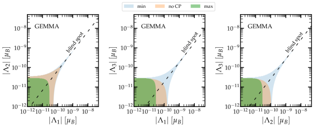
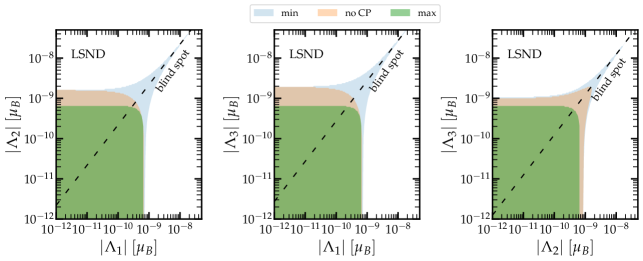
Figure 1: Upper row graphs: $90\%$ CL limits on Majorana neutrino transition magnetic and electric dipole moments in Bohr magneton units. The results are obtained for couplings in the mass eigenstate basis by mapping the upper bound on $\mu_{\nu_{e}}^{2}$ from the GEMMA reactor experiment Beda et al. (2012) to the fundamental parameters $\Lambda_{i}=\mu_{i}-i\epsilon_{i}$. Points along the colored regions saturate the GEMMA limit while those below correspond to smaller values. No CP means the CP phases in the electromagnetic sector are fixed to zero. Lower row graphs: Same as for graphs in the upper row but for bounds on $\mu_{\nu_{\mu}}^{2}$ from the LSND accelarator experiment Auerbach et al. (2001). Results from the DONUT upper limit on $\mu_{\nu_{\tau}}^{2}$ Schwienhorst et al. (2001) follow the same trend. Since they involve less stringent bounds are not displayed.

Graphs in the upper row in Fig. 1 show the results obtained by mapping the upper limit on $\mu_{\nu_{e}}^{2}$ from the GEMMA reactor experiment (Eqs. (11) and (17) with $\alpha=e$) to the parameter space of fundamental couplings (those entering in the Hamiltonian in Eq. (3)). Graphs in the lower row, instead, follow from limits on $\mu_{\nu_{\mu}}^{2}$ from the LSND experiment. Boundaries in the colored regions saturate the limit, while points within correspond to smaller values. Shown as well is the blind spot line along which $\mu_{\nu_{\alpha}}^{2}=0$ ($\alpha=e,\mu$). For parameters along that line, signals in a reactor or a short baseline accelerator experiment are absent regardless of the size of the fundamental couplings. Three regions in each $\Lambda_{i}-\Lambda_{j}$ plane can be identified. The green region is determined by vector alignments for which $\mu_{\nu_{e}}^{2}$ is maximized, as discussed previously. For this reason, in this region the most constrained parameters are found (the largest couplings have sizes of the order of the GEMMA or LSND limit). The blue region, in particular the spike along the blind spot line, follows from parameters that satisfy the alignment condition in Eq. (23) but that slightly departure from the conditions the $\Lambda_{i}$ should satisfy so to fall exactly in the blind spot. In this region couplings about two orders of magnitude larger than the GEMMA or LSND limit can be found, inline with our previous discussion as well.

To emphasize that the larger the couplings the more aligned the parameter space vectors $\Lambda_{ie}$ should be, we have as well included a region where the new interactions have vanishing CP phases (brown region). One can see that although larger couplings are allowed, compared with those in the green region, the largest possible values are not comparable to those in the region where CP phases are not zero. Finally, it is worth mentioning that the corresponding results for the $\mu_{\tau}^{2}$ coupling follow the same behavior, but since the upper limit is not as stringent as for the other two flavors, they are not displayed.

Experimental upper limits apply to the effective coupling $\mu_{\nu_{\alpha}}^{2}$ and do not necessarily imply small fundamental couplings, as demonstrated by the results in Fig. 1. This then raises the question of whether limits on the fundamental parameters implied by GEMMA can be reconciled with those that follow from the less severe LSND limit. From our discussion of blind spots, it is clear that despite the large mismatch of these experimental upper limits, regions in parameter space where this is the case indeed exist. For example, if couplings and phases are tuned according to the conditions of the $\mu_{\nu_{e}}^{2}$ blind spot, one finds $\mu_{\nu_{\mu}}^{2}=\mu_{\nu_{\mu}}^{2}|_{\text{max}}=|\vec{\Lambda}|^{2}$ . Thus, in this region no signal at GEMMA is expected regardless of the size of the couplings. GEMMA upper bound is therefore trivially satisfied and couplings with the appropriate size to satisfy as well the LSND bound are indeed possible. Fig. 2 shows the result of a scan in the parameter space where phases have been fixed such that alignments of the flavor vectors in $\mu_{\nu_{e}}^{2}$ are in place. This choice allows entering the region where the GEMMA limit can be satisfied with sufficiently large couplings and hence leads to regions in parameter space where couplings can simultaneously account for GEMMA and LSND measurements.

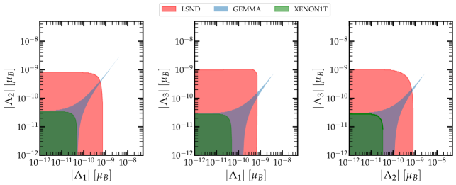
Figure 2: Effective electron and muon neutrino couplings contour plots in the planes of fundamental parameters $\Lambda_{i}=\mu_{i}-i\epsilon_{i}$ (in Bohr magneton units) in the mass eigenstate basis. These regions determine the $90\%$ CL limits on the Hamiltonian parameters, they follow from GEMMA, LSND and XENON1T measurements Beda et al. (2012); Auerbach et al. (2001); Aprile et al. (2020). These results demonstrate that regions in parameter space where GEMMA and LSND limits can be simultaneously satisfied exist.

IV.2 Effective couplings in solar neutrino experiments

We now turn to the discussion of the effective coupling pertaining solar neutrinos. In contrast to the reactor and short-baseline cases, this coupling acquires a rather simple form in the mass eigenstate basis, as can be seen from Eq. (13). Explicitly it reads

$$\mu_{\nu,\text{sol}}^{2}=\sum_{i=1}^{2}\left|\Lambda_{i}\right|^{2}\left[1-c_{13}^{2}P_{ei}^{2\nu}(E_{\nu})\right]+c_{13}^{2}\left|\Lambda_{3}\right|^{2}\,$$ (25)

where $P_{ei}^{2\nu}(E_{\nu})$ refers to the two-flavor scheme probability of observing the $i$-th mass eigenstate $\nu_{i}$ at the scattering point, given an initial electron neutrino state. No dependence on CP phases is found in this basis, and so experimental limits placed on this effective coupling only constrain the mass basis parameters $\Lambda_{i}$. The oscillation probabilities introduce as well an energy dependence. For electron-neutrino scattering experiments that dependence is to a large degree determined by the energy range of the solar pp process, while for CE$\nu$NS by the energy range of the ⁸B reaction. Since these processes peak at $\sim 0.4\,$MeV and $\sim 10\,$MeV respectively, one can then evaluate the probability for those energies and then map into parameter space.

$\vec{\Lambda}^{m}_{1}$		$\vec{\Lambda}^{m}_{2}$		$\vec{\Lambda}^{m}_{3}$
$\widehat{u}_{1e}\cdot\widehat{u}_{1\mu}$	$\cos(\varphi_{1}+\pi)$	$\widehat{u}_{2e}\cdot\widehat{u}_{2\mu}$	$\cos(\varphi_{1})$	$\widehat{u}_{3e}\cdot\widehat{u}_{3\mu}$	$\cos(\varphi_{1}+\pi)$
$\widehat{u}_{1e}\cdot\widehat{u}_{1\tau}$	$\cos(\varphi_{3}-\varphi_{1})$	$\widehat{u}_{2e}\cdot\widehat{u}_{2\tau}$	$\cos(\varphi_{3}-\varphi_{1})$	$\widehat{u}_{3e}\cdot\widehat{u}_{3\tau}$	$\cos(\varphi_{3}-\varphi_{1}+\pi)$
$\widehat{u}_{1\mu}\cdot\widehat{u}_{1\tau}$	$\cos(\varphi_{3})$	$\widehat{u}_{2\mu}\cdot\widehat{u}_{2\tau}$	$\cos(\varphi_{3})$	$\widehat{u}_{3\mu}\cdot\widehat{u}_{3\tau}$	$\cos(\varphi_{3})$

Table 4: Alignments of the parameter space vectors that define the neutrino magnetic effective coupling in the solar case in the flavor eigenstate basis (see Eqs. (26) and (27)). As in the reactor and short-baseline cases, they “measure” the amount of CP violation the new physics comes along with.

In the flavor basis the effective coupling becomes more intricate, but carries information on possible CP phases. As in the analysis of reactor and short-baseline experiments, in this case one can as well understand CP violation in terms of parameter space vectors misalignments. However, in contrast to what we have found in those cases, no alignments in parameter space exist such that blind spots can be accessed. The coupling in this basis can be written as

$$\mu_{\nu,\text{sol}}^{2}=\sum_{i=1}^{3}\left|\vec{\Lambda}_{i}^{\text{m}}\right|^{2}\left(1-c_{13}^{2}P_{ei}^{2\nu}\right)\qquad(\text{with}\,\,P_{e3}^{2\nu}=0)\ .$$ (26)

Here the oscillation probabilities follow the same meaning as in Eq. (25) and the parameter space vectors are defined according to

$$\vec{\Lambda}_{i}^{\text{m}}=\sum_{\alpha=e,\mu,\tau}\vec{\Lambda}_{i\alpha}^{\text{m}}=\sum_{\alpha=e,\mu,\tau}f_{i\alpha}\Lambda_{\alpha}\widehat{u}_{i\alpha}\ ,$$ (27)

where the superindex “m” has been introduced to differentiate these vectors from those in the reactor and short-baseline cases given in Eq. (18). Alignments, dictated by the scalar product of the unit vectors $\widehat{u}_{i\alpha}$, are displayed in Tab. 4. We have found that for certain alignments and parameter choices one of the three vectors $\vec{\Lambda}^{\text{m}}_{i}$ can be set to zero, however for that particular choice the other two do not vanish. Hence, we conclude that blind spots are not present in the solar neutrino case.

Results for the parameter space mapping using XENON1T results (interpreted as being generated by neutrino magnetic transitions) are shown in Fig. 3. The result has been obtained by fixing the CP phases such that one of the three terms in Eq. (26) vanishes. This demonstrates that although individually one of these terms can be set to zero by proper alignments (determined by the CP phases) a blind spot region does not exist. Accordingly, in view of solar neutrino data the mapping to parameter space will result always in parameters whose values amount to the same size of the corresponding measurement. This in sharp contrast to the reactor and short-baseline accelerator cases where the blind spot region allows for couplings with larger values.

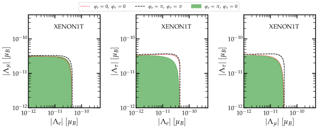
Figure 3: Parameter space regions in the $\Lambda_{\alpha}-\Lambda_{\beta}$ planes consistent with the $90\%$ CL range reported by XENON1T (understanding the excess as being generated by neutrino magnetic transitions) Aprile et al. (2020). Results are obtained for CP phases choices such that one of the terms in the effective neutrino magnetic moment coupling vanishes. This result demonstrates that even though individually one of the terms in $\mu_{\nu_{e}}^{2}$ can be taken to vanish through proper parameter space vector alignments (with suitable CP phases), upper limits on the couplings amount to the size of the experimental measurement.

V Dirac neutrino magnetic and electric dipole moments

Since the Majorana case allows only for transition moments, in this case we focus on purely magnetic and electric dipole moments. This means that in the Dirac coupling matrix in Eq. (5) we take the off-diagonal couplings to be zero. Couplings in the flavor basis follow from the relations in Eq. (6), and so all the entries of the coupling matrix in that basis are nonzero. In contrast to the Majorana case, in this particular Dirac scenario all couplings acquire a rather simple form in both bases. For reactor and short-baseline accelerator neutrinos in the mass basis one finds

$$\mu_{\nu_{\alpha}}^{2}=\left|\sum_{i=1}^{3}\vec{\lambda}_{i\alpha}\right|^{2}\ ,$$ (28)

where the parameter space vectors in this case read

$$\vec{\lambda}_{i\alpha}=f_{i\alpha}\lambda_{ii}\widehat{v}_{i}\ .$$ (29)

The unit vectors $\widehat{v}_{i}$ are orthonormal and the coefficients $f_{i\alpha}$ follow from Tab. 2. Note that in contrast to the results in the Majorana case, no destructive interference is found and so no dependence on CP phases. Thus, for Majorana neutrinos and reactor and short-baseline accelerator experiments, CP phases play a crucial role but none for purely magnetic and dipole moments (only possible in the Dirac case). In the flavor basis, again, expressions for the effective neutrino magnetic moments are reduced to rather simple form with no CP phases dependence as well:

$$\mu_{\nu_{\alpha}}^{2}=\sum_{\beta}\left|\lambda_{\alpha\beta}\right|^{2}\ .\qquad$$ (30)

For solar neutrinos in the mass basis the result is rather simple and as expected involves a dependence on the neutrino flavor oscillation probability

$$\mu_{\nu,\text{sol}}^{2}=\sum_{i=1}^{2}\left|\lambda_{ii}\right|^{2}\,c_{13}^{2}P_{ei}^{2\nu}-\left|\lambda_{33}\right|^{2}\,s_{13}^{2}\ ,\qquad$$ (31)

where as in the Majorana case, $P_{ei}^{2\nu}$ measures the probability of detection of the $i$-th neutrino mass eigenstate. Results for the flavor basis follow directly from Eq. (31) through

$$\lambda_{ii}=\left(U^{T}\cdot\lambda_{D}\cdot U\right)_{ii}\ .$$ (32)

From these results it becomes clear that each term in Eq. (31) involves CP phases, but given the structure of the full effective coupling no special features are found. Alignments might be found so a particular $|\lambda_{ii}|$ term vanishes, but those alignments will not lead to blind spots.

All in all, in the Dirac diagonal case (pure neutrino magnetic and electric dipole moments) no features as those found in the Majorana case (transitions) are observed. As a result, mapping of experimental data into parameter space implies couplings whose values are of the same order than the corresponding upper bounds (or an eventual actual measurement). Results of the mapping are shown in Fig. 4 which displays the 90% CL limits in the fundamental parameters derived by considering upper limits obtained from LSND Auerbach et al. (2001), GEMMA Beda et al. (2012) and XENON1T Aprile et al. (2020) neutrino-electron elastic scattering measurements.

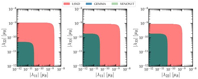
Figure 4: 90% CL limits on the Hamiltonian parameters in the case of Dirac neutrino magnetic and electric dipole moments (diagonal couplings) in the mass eigenstate basis. Results follow from experimental upper limits obtained from neutrino-electron elastic scattering processes at LSND Auerbach et al. (2001), GEMMA Beda et al. (2012) and XENON1T Aprile et al. (2020).

VI Conclusions

We have studied the behavior of effective neutrino magnetic and electric dipole moments (transitions) and their dependence with the Hamiltonian (fundamental) parameters, including CP phases in the new sector. We have considered the case of transitions for Majorana neutrinos and pure moments for Dirac neutrinos in both the mass and flavor eigenstate bases. Starting with a generic Dirac CP phase ($\delta$) we have focused on effective couplings valid for reactor and short-baseline neutrino experiments as well as for solar neutrino experiments.

We have shown that while individually the flavor effective couplings are basis dependent, the sum over flavor indices of the three different couplings is a basis invariant quantity. We thus have pointed out that if experimental information on the three flavors is available, the mapping of data to parameter space should be done using this quantity (see Eq. (16)). Otherwise, when interpreting data from a given experimental source in terms of fundamental parameters, the couplings to be used—in the absence of input on $\delta$—are those we have derived in Eqs. (11), (13), (14) and (15). If instead one fixes $\delta=\pi$, as suggested by neutrino global fits de Salas et al. (2018), a vector treatment of parameter space is possible and the effective couplings can be readily expressed in terms of fundamental parameters with the aid of the vectors defined by Eq. (18) (in the Majorana case) and Eq. (29) (in the Dirac case), along with the coefficients and alignments defined in Tabs. 2 and 4. These results provide then an experimental data mapping into parameter space as a straightforward procedure.

We have shown that while short-baseline and reactor couplings are sensitive to CP phases in the mass basis, the solar neutrino coupling is instead not. Conversely, in the flavor eigenstate basis short-baseline and reactor couplings are insensitive to possible CP phases, while the solar effective coupling acquires a CP-phase dependence. Though we have found that this behavior is valid regardless of the neutrino nature, the presence of CP violation does play a pivotal role in the Majorana case. We have demonstrated that it enables a blind spot region in parameter space, where the short-baseline or reactor effective couplings vanish even in the presence of nonvanishing large fundamental couplings. We, thus, have pointed out the need for analyses of multiple datasets to remove this regions in parameter space.

The presence of these blind spots open up regions where stringent limits, as those implied by GEMMA, can be satisfied with large Hamiltonian couplings. We have shown that this fact allows reconciling LSND and GEMMA upper limits which differ in about an order of magnitude. Here with reconciling we mean finding a common region where both experimental upper limits can be simultaneously saturated. We have finally demonstrated that in the Majorana case a tight short-baseline or reactor upper limit does not necessarily imply couplings of the order of the experimental bound.

Appendix A Phase average for the solar effective neutrino magnetic coupling

Since in the solar case interference terms come along with phases the effective parameter $\mu_{\nu_{\alpha}}$ has to be averaged over $L/E_{\nu}$ (the phases involved are $e^{\pm i(\Delta m^{2}_{ij}/2)(L/E_{\nu})}$, with $i=2,3$ and $j=1$). For the average one can take the normalized Gaussian smearing function

$$G(L/E_{\nu},\langle L/E_{\nu}\rangle,\sigma)=\frac{1}{\sqrt{2\pi\sigma^{2}}}\int d(L/E_{\nu})e^{-(L/E_{\nu}-\langle L/E_{\nu}\rangle)^{2}/2/\sigma^{2}}\ .$$ (33)

Average over the phases then reads

$$\langle e^{\pm i(\Delta m^{2}_{ij}/2)(L/E_{\nu})}\rangle=\frac{1}{\sqrt{2\pi\sigma^{2}}}\int d(L/E_{\nu})\,e^{\pm i(\Delta m^{2}_{ij}/2)(L/E_{\nu})}e^{-(L/E_{\nu}-\langle L/E_{\nu}\rangle)^{2}/2/\sigma^{2}}\ .$$ (34)

This integral can actually be calculated analytically by changing variables to

$$x=\frac{L}{E_{\nu}}\ ,\qquad\lambda=\frac{1}{2\sigma^{2}}\ ,\qquad x_{\pm}=x-\left(\langle x\rangle\pm i\frac{\Delta m_{ij}^{2}}{2}\sigma^{2}\right)\ .$$ (35)

In terms of these new variables and taking into account the standard result

$$\int dx\,e^{-\lambda x^{2}}=\sqrt{\frac{\pi}{\lambda}}\ ,$$ (36)

the result in Eq. (12) is obtained

$$\langle e^{\pm i(\Delta m^{2}_{ij}/2)(L/E_{\nu})}\rangle=e^{\pm(\Delta m^{2}_{ij}/2)\langle L/E_{\nu}\rangle}e^{-\Delta m_{ij}^{4}\langle L/E_{\nu}\rangle^{2}/8}\ .$$ (37)

Appendix B Effective couplings in the mass basis in terms of the lepton mixing matrix

In general, one can write the Majorana coupling matrix for the transition moments as follows (see Eq. (5))

$$\lambda^{\prime}_{ij}=\epsilon_{ijk}|\Lambda_{k}|e^{i\varphi_{k}}\ .$$ (38)

As already noticed, $\varphi_{2}$ (or any other phase) can be removed by means of an overall phase scaling of the neutrino fields vector, leaving behind only two physical CP phases. The notation in Eq. (38) enables writing the effective coupling in a rather simple form, namely. For a given neutrino flavor, $\alpha$, in the absence of neutrino flavor oscillations, the effective neutrino magnetic moment can be rewritten in terms of the lepton mixing matrix elements according to

$$\mu^{2}_{\nu_{\alpha}} = \sum_{i,j,l}U_{\alpha l}\,\lambda^{\prime\dagger}_{il}\,\lambda^{\prime}_{ij}\,U^{\dagger}_{j\alpha}$$ (39)

$$= \sum_{i,j,l}U_{\alpha l}U^{*}_{\alpha j}\left(-\epsilon_{lik}\epsilon_{ijm}|\Lambda_{k}||\Lambda_{m}|e^{-i\varphi_{k}}e^{i\varphi_{m}}\right)$$

$$= -\sum_{i,j,l}U_{\alpha l}U^{*}_{\alpha j}\left(\delta_{lm}\delta_{kj}-\delta_{lj}\delta_{km}\right)|\Lambda_{k}||\Lambda_{m}|e^{-i\varphi_{k}}e^{i\varphi_{m}}$$

$$= \left|\vec{\Lambda}\right|^{2}\sum_{l}U_{\alpha l}U^{*}_{\alpha j}-\sum_{j,l}\left(U^{*}_{\alpha j}|\Lambda_{j}|e^{-i\varphi_{j}}\right)\left(U_{\alpha l}|\Lambda_{l}|e^{i\varphi_{l}}\right)\ .$$

After taking into account the unitarity of the lepton mixing matrix and arranging the second term in Eq. (39), the effective neutrino magnetic moment in flavor $\alpha$ becomes

$$\mu^{2}_{\nu_{\alpha}}=\left|\vec{\Lambda}\right|^{2}-\sum_{j}{|U_{\alpha j}\Lambda_{j}|}^{2}-2\sum_{j>l}\mathbb{R}\text{e}\left[U^{*}_{\alpha j}U_{\alpha l}|\Lambda_{j}||\Lambda_{l}|e^{-i\varphi_{j}}e^{i\varphi_{l}}\right]\ .$$ (40)

From this result one can then see that proper alignments determined by particular choices of the CP phases allow the maximization of the coupling. More importantly, open the blind spot region discussed in Sec. IV. We can see that the previous equation can be written as

$$\mu^{2}_{\nu_{\alpha}}=\left|\vec{\Lambda}\right|^{2}-\left|\left(\sum_{j=1}^{3}\left|U_{\alpha j}\right|\left|\Lambda_{j}\right|\widehat{e}_{j\alpha}\right)\right|^{2}$$ (41)

with $\widehat{e}_{j\alpha}$ unit vectors such that

$$\widehat{e}_{i\alpha}\cdot\widehat{e}_{j\beta}=\delta_{\alpha\beta}\cos\left[-\arg{\left(U_{\alpha i}\right)}+\arg{\left(U_{\beta j}\right)}-\varphi_{i}+\varphi_{j}\right]\ .$$ (42)

In particular, for the case of $\delta=\pi$, we have the products $\widehat{e}_{i\alpha}\cdot\widehat{e}_{j\beta}$ given in Table 2.

References

- Giunti and Studenikin (2015) C. Giunti and A. Studenikin, Rev. Mod. Phys. 87, 531 (2015), eprint 1403.6344.
- Auerbach et al. (2001) L. B. Auerbach et al. (LSND), Phys. Rev. D 63, 112001 (2001), eprint hep-ex/0101039.
- Schwienhorst et al. (2001) R. Schwienhorst et al. (DONUT), Phys. Lett. B 513, 23 (2001), eprint hep-ex/0102026.
- Kosmas et al. (2015) T. S. Kosmas, O. G. Miranda, D. K. Papoulias, M. Tortola, and J. W. F. Valle, Phys. Rev. D 92, 013011 (2015), eprint 1505.03202.
- Miranda et al. (2019) O. G. Miranda, D. K. Papoulias, M. Tórtola, and J. W. F. Valle, JHEP 07, 103 (2019), eprint 1905.03750.
- Agostini et al. (2017) M. Agostini et al. (Borexino), Phys. Rev. D 96, 091103 (2017), eprint 1707.09355.
- Beda et al. (2012) A. G. Beda, V. B. Brudanin, V. G. Egorov, D. V. Medvedev, V. S. Pogosov, M. V. Shirchenko, and A. S. Starostin, Adv. High Energy Phys. 2012, 350150 (2012).
- Aprile et al. (2020) E. Aprile et al. (XENON), Phys. Rev. D 102, 072004 (2020), eprint 2006.09721.
- Hakenmüller et al. (2019) J. Hakenmüller et al., Eur. Phys. J. C 79, 699 (2019), eprint 1903.09269.
- Bonet et al. (2021) H. Bonet et al. (CONUS), Phys. Rev. Lett. 126, 041804 (2021), eprint 2011.00210.
- Aguilar-Arevalo et al. (2019) A. Aguilar-Arevalo et al. (CONNIE), Phys. Rev. D 100, 092005 (2019), eprint 1906.02200.
- Strauss et al. (2017) R. Strauss et al., Eur. Phys. J. C77, 506 (2017), eprint 1704.04320.
- Agnolet et al. (2017) G. Agnolet et al. (MINER), Nucl. Instrum. Meth. A 853, 53 (2017), eprint 1609.02066.
- Choi (2020) J. J. Choi, Proceedings of The 21st international workshop on neutrinos from accelerators — PoS(NuFact2019) (2020).
- Akimov et al. (2020) D. Y. Akimov et al. (RED-100), JINST 15, P02020 (2020), eprint 1910.06190.
- Billard et al. (2017) J. Billard et al., J. Phys. G 44, 105101 (2017), eprint 1612.09035.
- Wong (2015) H. T.-K. Wong, The Universe 3, 22 (2015), eprint 1608.00306.
- Flores et al. (2021) L. J. Flores et al. (SBC, CENS Theory Group at IF-UNAM), Phys. Rev. D 103, L091301 (2021), eprint 2101.08785.
- Baxter et al. (2020) D. Baxter et al., JHEP 02, 123 (2020), eprint 1911.00762.
- Aalbers et al. (2016) J. Aalbers et al. (DARWIN), JCAP 1611, 017 (2016), eprint 1606.07001.
- Aprile et al. (2016) E. Aprile et al. (XENON), JCAP 1604, 027 (2016), eprint 1512.07501.
- Akerib et al. (2020) D. S. Akerib et al. (LUX-ZEPLIN), Phys. Rev. D 101, 052002 (2020), eprint 1802.06039.
- Aristizabal Sierra et al. (2021a) D. Aristizabal Sierra, B. Dutta, D. Kim, D. Snowden-Ifft, and L. E. Strigari, Phys. Rev. D 104, 033004 (2021a), eprint 2103.10857.
- Aristizabal Sierra et al. (2020) D. Aristizabal Sierra, R. Branada, O. G. Miranda, and G. Sanchez Garcia, JHEP 12, 178 (2020), eprint 2008.05080.
- Shoemaker (2017) I. M. Shoemaker, Phys. Rev. D95, 115028 (2017), eprint 1703.05774.
- Shoemaker and Welch (2021) I. M. Shoemaker and E. Welch (2021), eprint 2103.08401.
- Denton et al. (2018) P. B. Denton, Y. Farzan, and I. M. Shoemaker, JHEP 07, 037 (2018), eprint 1804.03660.
- Aristizabal Sierra et al. (2019a) D. Aristizabal Sierra, B. Dutta, S. Liao, and L. E. Strigari, JHEP 12, 124 (2019a), eprint 1910.12437.
- Aristizabal Sierra et al. (2019b) D. Aristizabal Sierra, V. De Romeri, and N. Rojas, JHEP 09, 069 (2019b), eprint 1906.01156.
- Majumdar et al. (2021) A. Majumdar, D. K. Papoulias, and R. Srivastava (2021), eprint 2112.03309.
- Cadeddu et al. (2021) M. Cadeddu, N. Cargioli, F. Dordei, C. Giunti, Y. F. Li, E. Picciau, and Y. Y. Zhang, JHEP 01, 116 (2021), eprint 2008.05022.
- Dutta et al. (2017) B. Dutta, S. Liao, L. E. Strigari, and J. W. Walker, Phys. Lett. B773, 242 (2017), eprint 1705.00661.
- Aristizabal Sierra et al. (2018) D. Aristizabal Sierra, N. Rojas, and M. H. G. Tytgat, JHEP 03, 197 (2018), eprint 1712.09667.
- Aristizabal Sierra et al. (2021b) D. Aristizabal Sierra, V. De Romeri, L. J. Flores, and D. K. Papoulias (2021b), eprint 2109.03247.
- Fujikawa and Shrock (1980) K. Fujikawa and R. Shrock, Phys. Rev. Lett. 45, 963 (1980).
- Schechter and Valle (1981) J. Schechter and J. W. F. Valle, Phys. Rev. D 24, 1883 (1981), [Erratum: Phys.Rev.D 25, 283 (1982)].
- Pal and Wolfenstein (1982) P. B. Pal and L. Wolfenstein, Phys. Rev. D 25, 766 (1982).
- Kayser (1982) B. Kayser, Phys. Rev. D 26, 1662 (1982).
- Nieves (1982) J. F. Nieves, Phys. Rev. D 26, 3152 (1982).
- Shrock (1982) R. E. Shrock, Nucl. Phys. B 206, 359 (1982).
- Grimus and Schwetz (2000) W. Grimus and T. Schwetz, Nucl. Phys. B 587, 45 (2000), eprint hep-ph/0006028.
- Canas et al. (2016a) B. C. Canas, O. G. Miranda, A. Parada, M. Tortola, and J. W. F. Valle, Phys. Lett. B 753, 191 (2016a), [Addendum: Phys.Lett.B 757, 568–568 (2016)], eprint 1510.01684.
- Vogel and Engel (1989) P. Vogel and J. Engel, Phys. Rev. D39, 3378 (1989).
- Grimus and Stockinger (1998) W. Grimus and P. Stockinger, Phys. Rev. D 57, 1762 (1998), eprint hep-ph/9708279.
- Beacom and Vogel (1999) J. F. Beacom and P. Vogel, Phys. Rev. Lett. 83, 5222 (1999), eprint hep-ph/9907383.
- Papoulias and Kosmas (2015) D. K. Papoulias and T. S. Kosmas, Phys. Lett. B 747, 454 (2015), eprint 1506.05406.
- Giunti and Kim (2007) C. Giunti and C. W. Kim, Fundamentals of Neutrino Physics and Astrophysics (OXFORD, 2007), ISBN 978-0-19-850871-7.
- Miranda et al. (2020) O. G. Miranda, D. K. Papoulias, M. Tórtola, and J. W. F. Valle, Phys. Lett. B 808, 135685 (2020), eprint 2007.01765.
- Miranda et al. (2021) O. G. Miranda, D. K. Papoulias, O. Sanders, M. Tórtola, and J. W. F. Valle (2021), eprint 2109.09545.
- de Salas et al. (2021) P. F. de Salas, D. V. Forero, S. Gariazzo, P. Martínez-Miravé, O. Mena, C. A. Ternes, M. Tórtola, and J. W. F. Valle, JHEP 02, 071 (2021), eprint 2006.11237.
- Acciarri et al. (2015) R. Acciarri et al. (DUNE) (2015), eprint 1512.06148.
- Abe et al. (2018) K. Abe et al. (Hyper-Kamiokande), PTEP 2018, 063C01 (2018), eprint 1611.06118.
- Cao et al. (2014) J. Cao et al., Phys. Rev. ST Accel. Beams 17, 090101 (2014), eprint 1401.8125.
- Tang et al. (2019) J. Tang, S. Vihonen, and T.-C. Wang, JHEP 12, 130 (2019), eprint 1909.01548.
- Canas et al. (2016b) B. C. Canas, O. G. Miranda, A. Parada, M. Tortola, and J. W. F. Valle, J. Phys. Conf. Ser. 761, 012043 (2016b), eprint 1609.08563.
- de Salas et al. (2018) P. F. de Salas, D. V. Forero, C. A. Ternes, M. Tortola, and J. W. F. Valle, Phys. Lett. B782, 633 (2018), eprint 1708.01186.