Tridiagonal Maximum-Entropy Sampling
and Tridiagonal Masks$\vphantom{|}{}^{1}$

Abstract

The NP-hard maximum-entropy sampling problem (MESP) seeks a maximum (log-)determinant principal submatrix, of a given order, from an input covariance matrix $C$.

We give an efficient dynamic-programming algorithm for MESP when $C$ (or its inverse) is tridiagonal and generalize it to the situation where the support graph of $C$ (or its inverse) is a spider graph with a constant number of legs (and beyond). We give a class of arrowhead covariance matrices $C$ for which a natural greedy algorithm solves MESP.

A mask $M$ for MESP is a correlation matrix with which we pre-process $C$, by taking the Hadamard product $M\circ C$. Upper bounds on MESP with $M\circ C$ give upper bounds on MESP with $C$. Most upper-bounding methods are much faster to apply, when the input matrix is tridiagonal, so we consider tridiagonal masks $M$ (which yield tridiagonal $M\circ C$). We make a detailed analysis of such tridiagonal masks, and develop a combinatorial local-search based upper-bounding method that takes advantage of fast computations on tridiagonal matrices.

1 Introduction

Let $C$ be an order-$n$ symmetric positive semidefinite real matrix, and let $s$ be an integer satisfying $1\leq s\leq n$. In applications, $C$ is the covariance matrix for a multivariate Gaussian random vector $Y_{N_{n}}$, where $N_{n}:=[1,n]:=\{1,2,\ldots,n\}$ — note that we regard $N_{n}$ as an ordered set, which will be important later. For nonempty $S\subseteq N_{n}$, let $C[S,S]$ denote the principal submatrix of $C$ indexed by $S$. We denote $\log\det(\cdot)$ by $\operatorname{ldet}(\cdot)$. Up to constants, $\operatorname{ldet}C[S,S]$ is the (differential) entropy associated with the subvector $Y_{S}$ (see [SW], for example). The maximum-entropy sampling problem, defined by [SW], is

$$z=\max~{}\left\{\operatorname{ldet}C[S,S]~{}:~{}|S|=s,~{}S\subseteq N_{n}\right\}$$ (MESP)

MESP corresponds to choosing a maximum-entropy subvector $Y_{S}$ from $Y_{N}$, subject to $|S|=s$. Later, it will sometimes be convenient to emphasize the dependence of MESP on the data, and in such situations we will write MESP$(C,s)$ and $z(C,s)$.

MESP was introduced in [SW], it was established to be NP-Hard in [KLQ] (via reduction from the NP-Complete problem: does an $n$-vertex graph $G$ have a vertex packing of cardinality $s$), and there has been considerable work on algorithms. Viable approaches aimed at exact solution of moderate-sized instances employ branch-and-bound (see [KLQ]). For use in branch-and-bound, we have many methods for efficiently calculating good upper bounds; see [KLQ, AFLW_IPCO, AFLW_Using, HLW, LeeWilliamsILP, AnstreicherLee_Masked, BurerLee, Anstreicher_BQP_entropy, Kurt_linx, Mixing, Nikolov, Weijun, fact] and the survey [LeeEnv]. Notably, we have developed an R package providing an easy means for instantiating MESP from raw environmental-monitoring data (see [Rpackage, Al-ThaniLee1]).

In what follows, “$\circ$” denotes Hadamard (i.e., elementwise) product of a pair of matrices of the same dimensions. Given a positive integer $n$, we define a mask as any $n\times n$ symmetric positive semidefinite matrix $M$ with all ones on the diagonal. Masks are better known as “correlation matrices”. These were introduced for MESP in [AnstreicherLee_Masked], where it was observed that for any $S$ and mask $M$, $\operatorname{ldet}C[S,S]\leq\operatorname{ldet}(C\circ M)[S,S]$, and so any upper bound on MESP for $C\circ M$ is valid for the MESP on $C$. It is a challenge to find a good mask with respect to a particular MESP upper-bounding method — i.e., a mask $M$ that minimizes the upper bound on $z(C\circ M,s)$. This topic was investigated in [AnstreicherLee_Masked] and [BurerLee]. We define a combinatorial mask as any block-diagonal mask $M$ where the diagonal blocks (which may vary in size) are matrices of all ones. At the extremes, we have $M:=I_{n}$ (an identity matrix) and $M=:J_{n}$ (an all ones matrix). As we observed in [AnstreicherLee_Masked], we can view some of [HLW] and [LeeWilliamsILP] in this way; e.g., the “spectral partition bound” of [HLW]. But there are many possibilities for masks that are not combinatorial masks. For example, a (tridiagonal) $\frac{1}{2}$-mask $M$ has $M_{i,i+1}=M_{i+1,i}:=\frac{1}{2}$ for $i=1,\ldots,n-1$ (and all other off-diagonal entries are 0). One goal of ours is to investigate computational aspects of tridiagonal masks $M$, so as to take advantage of the fact that most bounds can be calculated much faster (than on dense matrices) for tridiagonal matrices (in our case, $M\circ C$).

In Section 2, we give an $\mathcal{O}(n^{5})$ dynamic-programming algorithm for MESP when $C$ is tridiagonal. This also solves the problem in the same complexity when instead $C^{-1}$ is tridiagonal. This is the first progress on identifying significant polynomially-solvable cases of MESP. We extend our result to the case where the support graph of $C$ is a spider with a constant number of legs, and we indicate how it can be further extended when the number of connected components of the support graph of $C$ is polynomial in $n$. Finally, we present the results of computational experiments on matrices having support graphs that are spiders, indicating the superiority of a parallel implementation of our dynamic-programming algorithm as compared with branch-and-bound.

In Section 3, we characterize a class of positive-semidefinite “arrowhead matrices” (i.e., having the support graph of $C$ being a star), such that a certain natural greedy algorithm optimally solves MESP.

In Section LABEL:sec:tridiagM, we characterize for each $n$, masks that differ from $\frac{1}{2}$-masks in two (symmetric) pairs of off-diagonal positions. These results are useful in identifying good masks for MESP bounds, in the context of local search in the space of masks.

In Section LABEL:sec:masklocalsearch, we develop a combinatorial local-search algorithm that seeks a good tridiagonal mask $M$ for the so-called ‘linx’ upper bound (which is one of the best known upper-bounding method for MESP). Some computational experiments validate our approach.

2 Tridiagonal covariance matrices

The inverse covariance matrix, known as the precision matrix, captures the conditional covariances between pairs of random variables, conditioning on the remaining $n-2$ random variables. For a spatial process with random variables placed in a line, a reasonable model may have the precision matrix being tridiagonal, when the random variables are numbered in a natural order (along the line); intuitively, such a model would assume that no extra information can be obtained from a non-neighbor of a random variable $Y_{i}$, over and above the information obtainable from the neighbors of $Y_{i}$.

To see how the inverse covariance matrix plays a role for MESP, we employ the identity

$$\det C[S,S]=\det C\times\det C^{-1}[N_{n}\setminus S,N_{n}\setminus S]$$

(see [HJBook, Section 0.8.4]). With this identity, we have $z(C,s)=\operatorname{ldet}C+z(C^{-1},n-s)$, and so the MESP for choosing $s$ elements with respect to $C$ is equivalent to the MESP for choosing $n-s$ elements with respect to $C^{-1}$.

The determinant of a tridiagonal matrix can be calculated in linear time, via a simple recursion (see [demmel1997]), which we write for the symmetric case as that is our need. Let $T_{1}=(a_{1})$, and for $r\geq 2$, let

$$T_{r}:=\left(\begin{array}[]{ccccc}a_{1}&b_{1}&&&\\ b_{1}&a_{2}&b_{2}&&\\ &b_{2}&\ddots&\ddots&\\ &&\ddots&\ddots&b_{r-1}\\ &&&b_{r-1}&a_{r}\\ \end{array}\right).$$

Lemma 1.

Defining $\det T_{0}:=1$, we have $\det T_{r}=:a_{r}\det T_{r-1}-b_{r-1}^{2}\det T_{r-2}$, for $r\geq 2$.

Theorem 2.

MESP is polynomially solvable when $C$ or $C^{-1}$ is tridiagonal, or when there is a symmetric permutation of $C$ or $C^{-1}$ so that it is tridiagonal.

Proof.

Suppose that $C$ is tridiagonal. Let $S$ be an ordered subset of $N_{n}$. Then we can write $C[S,S]$ uniquely as $C[S,S]=\operatorname{Diag}(C[S_{1},S_{1}],C[S_{2},S_{2}],\ldots,C[S_{p},S_{p}])$, with $p\geq 1$, where each $S_{i}$ is a maximal ordered contiguous subset of $S$, and for all $1\leq i<j\leq p$, all elements of $S_{i}$ are less than all elements of $S_{j}$. We call the $S_{i}$ the pieces of $S$, and in particular $S_{p}$ is the last piece. It is easy to see that

$$\det C[S,S]=\textstyle\prod_{i=1}^{p}\det C[S_{i},S_{i}]=\det C[S_{p},S_{p}]\times\det C[S\setminus S_{p},S\setminus S_{p}]~{}.$$

Of course every $S$ has a last piece, and for an optimal $S$ to MESP, if the last piece is $S_{p}=:[k,\ell]$, then we have the “principle of optimality”:

$$\operatorname{ldet}C[S\setminus[k,\ell],S\setminus[k,\ell]]=z(C[N_{k-2},N_{k-2}],s-(\ell-k+1)).$$

With this way of thinking, we define

$$f(k,\ell,t):= \max\Big{\{}\operatorname{ldet}C[S,S]~{}:~{}$$

$$\qquad\qquad|S|=t,~{}S\subset N_{n}~{},\mbox{ and the last piece of $S$ is }[k,\ell]\Big{\}},$$

for $1\leq\ell-k+1\leq t\leq s$. Note that the last block of $S$ (in the definition of $f$) has $\ell-k+1$ elements, which is why $t$ must be at least that large. We have that

$$z(C,s)=\max_{k,\ell}\left\{f(k,\ell,s)~{}:~{}1\leq k\leq\ell\leq n,~{}\ell-k+1\leq s\right\},$$

where we are simply maximizing over the possible (quadratic number of) last pieces.

Our dynamic-programming recursion is

$$f(k,\ell,t)=\operatorname{ldet}C[[k,\ell],[k,\ell]]+ \max_{i,j}\left\{f(i,j,t-(\ell-k+1))~{}:~{}\right.$$

$$\left.1\leq i\ \leq j\leq k-2,~{}j-i+1\leq t-(\ell-k+1)\right\},$$

The idea is that if $[k,\ell]$ is the last block of an optimal selection of $t$ elements, then we have to pick $t-(\ell-k+1)$ more elements, and element $k-1$ is ruled out (because $[k,\ell]$ is maximal).

To get the recursion started, we calculate

$$f(k,\ell,\ell-k+1)=\operatorname{ldet}C[[k,\ell],[k,\ell]],$$

for $1\leq k\leq\ell\leq n$, $\ell-k+1\leq s$, observing that in such a boundary case, there is only one feasible solution. Already, it appears that the initialization requires $\mathcal{O}(n^{5})$ basic arithmetic operations, but in fact we can do this part in $\mathcal{O}(n^{2})$ operations, using the tridiagonal-determinant formula (Lemma 1).

Next, we compute, using the recursion, for $t=1,2,\ldots,s$, $f(k,\ell,t)$ for all $1\leq k\leq\ell\leq n$ such that $\ell-k+1<t$. It is not hard to see that this gives an $\mathcal{O}(n^{5})$ algorithm for MESP, when $C$ is tridiagonal, and by earlier observations, we also get an $\mathcal{O}(n^{5})$ algorithm for MESP, when $C^{-1}$ is tridiagonal. ∎

For an arbitrary symmetric $C$, with rows and columns indexed from $N_{n}$ , we consider the support graph $G(C)$, with node set $V(G[C]):=N_{n}$ , and edge set $E(G(C)):=\{(i,j)~{}:~{}i,j\in N_{n}\thinspace,~{}i<j,~{}C[i,j]\not=0\}$. If $C$ is a generic tridiagonal matrix (i.e., $C[i,i+1]\not=0$ for $i\in N_{n-1}$), then $G(C)$ is the path $P_{n}:=$ – – $\cdots$– . If $C$ is tridiagonal but not generic, then $G(C)$ is a subgraph of $P_{n}$ . Because we can efficiently solve MESP when $C$ is tridiagonal (and also when $C$ is tridiagonal after symmetric permutation), it is natural to consider broader classes of $C$, and natural exploitable structure is encoded in the support graph $G(C)$.

We are interested in “spiders” with $r\geq 1$ legs on an n-vertex set (see [MARTIN2008], for example): for convenience, we let the vertex set be $N_{n}$, and let vertex 1 be the body of the spider; the non-body vertex set $V_{i}$ of leg $i$, is a non-empty contiguously numbered subset of $N_{n}\setminus\{1\}$, such that distinct $V_{i}$ do not intersect, and the union of all $V_{i}$ is $N_{n}\setminus\{1\}$; we number the legs $i$ in such a way that: (i) the minimum element of $V_{1}$ is 2, and (ii) the minimum element of $V_{i+1}$ is one plus the maximum element of $V_{i}$, for $i\in[1,r-1]$. A small example clarifies all of this; see Figures 1–2. Note that with one leg, the spider is the path $P_{n}$ , and with two legs, the vertices can be re-numbered so that the the spider is the path $P_{n}$ . So, we may as well assume that the spider has $r\geq 3$ legs.

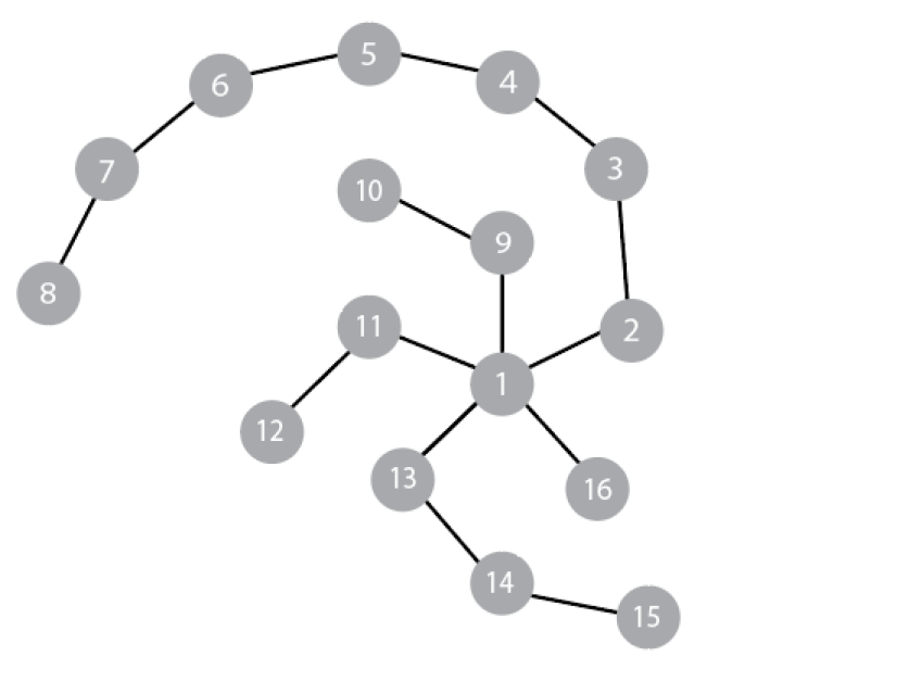
Figure 1: Spider with five legs

$$\left[\begin{array}[]{cccccccccccccccc}\scriptscriptstyle{(1,1)}&\scriptscriptstyle{(1,2)}&\scriptstyle{0}&\scriptstyle{0}&\scriptstyle{0}&\scriptstyle{0}&\scriptstyle{0}&\scriptstyle{0}&\scriptscriptstyle{(1,9)}&\scriptstyle{0}&\scriptscriptstyle{(1,11)}&\scriptstyle{0}&\scriptscriptstyle{(1,13)}&\scriptstyle{0}&\scriptstyle{0}&\scriptscriptstyle{(1,16)}\\ \scriptscriptstyle{(2,1)}&\scriptscriptstyle{(2,2)}&\scriptscriptstyle{(2,3)}&\scriptstyle{0}&\scriptstyle{0}&\scriptstyle{0}&\scriptstyle{0}&\scriptstyle{0}&\scriptstyle{0}&\scriptstyle{0}&\scriptstyle{0}&\scriptstyle{0}&\scriptstyle{0}&\scriptstyle{0}&\scriptstyle{0}&\scriptstyle{0}\\ \scriptstyle{0}&\scriptscriptstyle{(3,2)}&\scriptscriptstyle{(3,3)}&\scriptscriptstyle{(3,4)}&\scriptstyle{0}&\scriptstyle{0}&\scriptstyle{0}&\scriptstyle{0}&\scriptstyle{0}&\scriptstyle{0}&\scriptstyle{0}&\scriptstyle{0}&\scriptstyle{0}&\scriptstyle{0}&\scriptstyle{0}&\scriptstyle{0}\\ \scriptstyle{0}&\scriptstyle{0}&\scriptscriptstyle{(4,3)}&\scriptscriptstyle{(4,4)}&\scriptscriptstyle{(4,5)}&\scriptstyle{0}&\scriptstyle{0}&\scriptstyle{0}&\scriptstyle{0}&\scriptstyle{0}&\scriptstyle{0}&\scriptstyle{0}&\scriptstyle{0}&\scriptstyle{0}&\scriptstyle{0}&\scriptstyle{0}\\ \scriptstyle{0}&\scriptstyle{0}&\scriptstyle{0}&\scriptscriptstyle{(5,4)}&\scriptscriptstyle{(5,5)}&\scriptscriptstyle{(5,6)}&\scriptstyle{0}&\scriptstyle{0}&\scriptstyle{0}&\scriptstyle{0}&\scriptstyle{0}&\scriptstyle{0}&\scriptstyle{0}&\scriptstyle{0}&\scriptstyle{0}&\scriptstyle{0}\\ \scriptstyle{0}&\scriptstyle{0}&\scriptstyle{0}&\scriptstyle{0}&\scriptscriptstyle{(6,5)}&\scriptscriptstyle{(6,6)}&\scriptscriptstyle{(6,7)}&\scriptstyle{0}&\scriptstyle{0}&\scriptstyle{0}&\scriptstyle{0}&\scriptstyle{0}&\scriptstyle{0}&\scriptstyle{0}&\scriptstyle{0}&\scriptstyle{0}\\ \scriptstyle{0}&\scriptstyle{0}&\scriptstyle{0}&\scriptstyle{0}&\scriptstyle{0}&\scriptscriptstyle{(7,8)}&\scriptscriptstyle{(7,7)}&\scriptscriptstyle{(7,8)}&\scriptstyle{0}&\scriptstyle{0}&\scriptstyle{0}&\scriptstyle{0}&\scriptstyle{0}&\scriptstyle{0}&\scriptstyle{0}&\scriptstyle{0}\\ \scriptstyle{0}&\scriptstyle{0}&\scriptstyle{0}&\scriptstyle{0}&\scriptstyle{0}&\scriptstyle{0}&\scriptscriptstyle{(8,7)}&\scriptscriptstyle{(8,8)}&\scriptstyle{0}&\scriptstyle{0}&\scriptstyle{0}&\scriptstyle{0}&\scriptstyle{0}&\scriptstyle{0}&\scriptstyle{0}&\scriptstyle{0}\\ \scriptscriptstyle{(9,1)}&\scriptstyle{0}&\scriptstyle{0}&\scriptstyle{0}&\scriptstyle{0}&\scriptstyle{0}&\scriptstyle{0}&\scriptstyle{0}&\scriptscriptstyle{(9,9)}&\scriptscriptstyle{(9,10)}&\scriptstyle{0}&\scriptstyle{0}&\scriptstyle{0}&\scriptstyle{0}&\scriptstyle{0}&\scriptstyle{0}\\ \scriptstyle{0}&\scriptstyle{0}&\scriptstyle{0}&\scriptstyle{0}&\scriptstyle{0}&\scriptstyle{0}&\scriptstyle{0}&\scriptstyle{0}&\scriptscriptstyle{(10,9)}&\scriptscriptstyle{(10,10)}&\scriptstyle{0}&\scriptstyle{0}&\scriptstyle{0}&\scriptstyle{0}&\scriptstyle{0}&\scriptstyle{0}\\ \scriptscriptstyle{(11,1)}&\scriptstyle{0}&\scriptstyle{0}&\scriptstyle{0}&\scriptstyle{0}&\scriptstyle{0}&\scriptstyle{0}&\scriptstyle{0}&\scriptstyle{0}&\scriptstyle{0}&\scriptscriptstyle{(11,11)}&\scriptscriptstyle{(11,12)}&\scriptstyle{0}&\scriptstyle{0}&\scriptstyle{0}&\scriptstyle{0}\\ \scriptstyle{0}&\scriptstyle{0}&\scriptstyle{0}&\scriptstyle{0}&\scriptstyle{0}&\scriptstyle{0}&\scriptstyle{0}&\scriptstyle{0}&\scriptstyle{0}&\scriptstyle{0}&\scriptscriptstyle{(12,11)}&\scriptscriptstyle{(12,12)}&\scriptstyle{0}&\scriptstyle{0}&\scriptstyle{0}&\scriptstyle{0}\\ \scriptscriptstyle{(13,1)}&\scriptstyle{0}&\scriptstyle{0}&\scriptstyle{0}&\scriptstyle{0}&\scriptstyle{0}&\scriptstyle{0}&\scriptstyle{0}&\scriptstyle{0}&\scriptstyle{0}&\scriptstyle{0}&\scriptstyle{0}&\scriptscriptstyle{(13,13)}&\scriptscriptstyle{(13,14)}&\scriptstyle{0}&\scriptstyle{0}\\ \scriptstyle{0}&\scriptstyle{0}&\scriptstyle{0}&\scriptstyle{0}&\scriptstyle{0}&\scriptstyle{0}&\scriptstyle{0}&\scriptstyle{0}&\scriptstyle{0}&\scriptstyle{0}&\scriptstyle{0}&\scriptstyle{0}&\scriptscriptstyle{(14,13)}&\scriptscriptstyle{(14,14)}&\scriptscriptstyle{(14,15)}&\scriptstyle{0}\\ \scriptstyle{0}&\scriptstyle{0}&\scriptstyle{0}&\scriptstyle{0}&\scriptstyle{0}&\scriptstyle{0}&\scriptstyle{0}&\scriptstyle{0}&\scriptstyle{0}&\scriptstyle{0}&\scriptstyle{0}&\scriptstyle{0}&\scriptstyle{0}&\scriptscriptstyle{(15,14)}&\scriptscriptstyle{(15,15)}&\scriptstyle{0}\\ \scriptscriptstyle{(16,1)}&\scriptstyle{0}&\scriptstyle{0}&\scriptstyle{0}&\scriptstyle{0}&\scriptstyle{0}&\scriptstyle{0}&\scriptstyle{0}&\scriptstyle{0}&\scriptstyle{0}&\scriptstyle{0}&\scriptstyle{0}&\scriptstyle{0}&\scriptstyle{0}&\scriptstyle{0}&\scriptscriptstyle{(16,16)}\end{array}\right]$$

Figure 2: Matrix structure corresponding to Figure 1

Consider how a MESP solution $S$ intersects with the vertices of the spider. As before, the solution has pieces. Note how at most one piece contains the body, and every other piece is a contiguous set of vertices of a leg. The number of distinct possible pieces containing the body is $\mathcal{O}(n^{r})$. And the number of other pieces is $\mathcal{O}(n^{2})$. Overall, we have $\mathcal{O}(n^{r})$ pieces. In any solution, we can order the pieces by the minimum vertex in each piece. Based on this, we have a well defined last piece. From this, we can devise an efficient dynamic-programming algorithm, when we consider $r$ to be constant.

Theorem 3.

MESP is polynomially solvable when $G(C)$ or $G(C^{-1})$ is a spider with a constant number of legs.

In fact, we can easily organize a dynamic-programming scheme to exploit parallel computation. We can compute $\operatorname{ldet}C[S_{1},S_{1}]$ for all possible pieces containing the body 1. In parallel, we can compute optimal MESP solution values for all possible budgets $t\leq s$ for each leg, keeping track of the minimum vertex used for each such solution. With all of that information, we can then calculate an overall optimal solution.

We conducted some experiments to get some evidence that our dynamic-programming algorithm can be practical, compared to branch-and-bound. For each of $k=13,18,23,28,33,38,43$, we constructed ten positive-semidefinite matrices $C$, with $G(C)$ being a spider with three legs and $k$ vertices per leg. So we have $n=3k+1$, and we chose $s\sim\ell n/4$, for $\ell=1,2,3$. For the matrix constructions, we built a cvx (see [cvx]) semidefinite-programming model that takes a random choice of positive diagonal elements (constructed using rand of Matlab). The objective of the semidefinite-program was to maximize the sum of the off-diagonal elements of $C$, subject to $C$ is positive semidefinite, and $G(C)$ being the spider described above.

In Table 3, we report on our numerical experiments. We compare our parallel dynamic-programming algorithm, implemented in Matlab, with the serial branch-and-bound Matlab code of [Kurt_linx], which in turn uses the conic solver SDPT3 (see [Toh2012, SDPT3]). For our dynamic-programming algorithm, we use the Matlab parallel for-loop instruction parfor, for easy parallelization across spider legs. Parallelizing branch-and-bound would be a much more difficult task, and load balancing is highly nontrivial. We note that the running time of Matlab is highly variable (particularly for branch-and-bound), even with the same data and deterministic implementations of the algorithms. But because we average over ten experiments for each choice of $n$ and $s$, our results are meaningful. In the individual experiments it is clear that the dynamic-programming algorithm has more consistent time performance, while the time taken by the branch-and-bound fluctuates considerably. For most of the experiments, we set an upper limit of 2 hours (7200 seconds), except for the hardest one, the $n=130$, $s=97$ experiment, where we increased the time limit to 4 hours. In the table, $*$ indicates that the time limit was reached. Overall the dynamic-programming algorithm performed much better than branch-and-bound, and it scales much better.

		No. of	Avg. time for	Avg. time for
n (k)	s	trials	DP (sec.)	B&B (sec.)
40 (13)	10	10	$<1$	90
40 (13)	20	10	5	21
40 (13)	30	10	7	678
55 (18)	13	10	1	5642
55 (18)	27	10	21	173
55 (18)	41	10	33	8150
70 (23)	17	10	4	$7200^{*}$
70 (23)	35	10	86	241
70 (23)	52	10	146	$7200^{*}$
85 (28)	21	10	12	$7200^{*}$
85 (28)	42	10	260	347
85 (28)	63	10	519	$7200^{*}$
100 (33)	25	10	32	$7200^{*}$
100 (33)	50	10	858	$7200^{*}$
100 (33)	75	10	1364	$7200^{*}$
115 (38)	28	10	68	$7200^{*}$
115 (38)	57	10	1654	$7200^{*}$
115 (38)	86	10	3250	$7200^{*}$
130 (43)	32	10	163	$7200^{*}$
130 (43)	65	10	4086	$7200^{*}$
130 (43)	97	10	7093	$14400^{*}$

Table 3: DP vs B&B on spiders

Finally, we observe that for any class of $n$-vertex graphs for which the number of connected components is bounded above by a polynomial in $n$, we can use the same ideas as above to build an efficient dynamic-programming algorithm, assuming that we can enumerate the connected components in polynomial time. We do note that the class of $n$-vertex “stars” (i.e., spiders with $n-1$ single-edge legs) has $2^{n-1}$ subtrees containing the body, and so we do not in this way get an efficient algorithm for MESP when $G(C)$ is a star. But see the next section for an efficient algorithm for a subclass of the positive-semidefinite $C$ for which $G(C)$ is a star.

We could perhaps hope that what is generally needed for a tree (to lead to an efficient dynamic programming algorithm of this type) is a degree bound. But even for a degree bound of three, we get bad behavior: for binary trees, the number of subtrees can be exponential in the number of vertices.

3 Stars

In this section, we present an algorithm that computes the exact optimum of MESP, when $C$ is an arrowhead matrix (i.e., when the support graph $G(C)$ is a star with center 1) under an easily-checkable sufficient condition.

We define the arrowhead matrix

$$A(\alpha_{1},\alpha,D):=\left(\begin{array}[]{cc}\alpha_{1}&\alpha^{\mathchoice{\raisebox{0.0pt}{$\displaystyle\mathsf{T}$}}{\raisebox{0.0pt}{$\textstyle\mathsf{T}$}}{\raisebox{0.0pt}{$\scriptstyle\mathsf{T}$}}{\raisebox{0.0pt}{$\scriptscriptstyle\mathsf{T}$}}}\\ \alpha&D\end{array}\right),$$

with $\alpha_{1}\in\mathbb{R}$, $\alpha:=(\alpha_{2},\ldots,\alpha_{n})\in\mathbb{R}^{n-1}$, $d:=(d_{2},\ldots,d_{n})\in\mathbb{R}_{+}^{n-1}$, and $D:=\operatorname{Diag}(d)\in\mathbb{R}^{(n-1)\times(n-1)}$; see [arrow], for example.

Lemma 4.

$A(\alpha_{1},\alpha,D)\succeq 0$ if and only if $\alpha_{1}\geq\sum_{i=2}^{n}{\frac{\alpha_{i}^{2}}{d_{i}}}$.

Proof.

By symmetric row/column scaling, it is easy to see that $A(\alpha_{1},\alpha,D)\succeq 0$ if and only if $A(\alpha_{1},\tilde{\alpha},\alpha_{1}I)\succeq 0$, where $\tilde{\alpha}_{i}:=\alpha_{i}\sqrt{\frac{\alpha_{1}}{d_{i}}}$, for $i=2,\ldots,n$. From [AlizGold], we have that $A(\alpha_{1},\tilde{\alpha},\alpha_{1}I)\succeq 0$ if and only if $\alpha_{1}\geq\|\tilde{\alpha}\|$ — this is how the “ice-cream cone” constraint is typically modeled as a semidefinite-programming constraint. Now plugging in the definition of $\tilde{\alpha}$ and simplifying, we obtain our result. ∎

We consider now MESP$(A(\alpha_{1},\alpha,D),s)$, where we assume that $\alpha_{1}\geq\sum_{i=2}^{n}{\frac{\alpha_{i}^{2}}{d_{i}}}$, so that $A(\alpha_{1},\alpha,D)\succeq 0$. We will employ a greedy algorithm to solveMESP$(A(\alpha_{1},\alpha,D),s)$, but we do not simply apply such an algorithm directly. Rather, we will branch on element 1, and then apply a greedy algorithm to the two subproblems, selecting the best solution so found.

Our greedy algorithm is a manifestation of a generic greedy maximization algorithm for the more general problem: Given $f:2^{N}\mapsto\mathbb{R}$, find an $s$ element set $S\subset N$ with maximum value of $f(S)$.

Input: $f:2^{N}\mapsto\mathbb{R}$; $1<s<n$;

Output: $S$;

$S:=\emptyset$;

while $|S|<s$ do

       let $j^{*}:=\operatorname*{argmax}\big{\{}f(S+j~{}:~{}j\in N\setminus S\big{\}}$;

       let $S:=S+j$;

      

end while

Algorithm 1 Generic greedy for $\max\left\{f(S)~{}:~{}|S|=s\right\}$

We let $S_{0}=\emptyset,S_{1},\ldots,S_{s}$, be the sequence of iterates $S$ that are created, iteration by iteration, in Algorithm 1. We have the following nice property that we can exploit.

Lemma 5.

Suppose that $f:2^{N}\mapsto\mathbb{R}$ satisfies the following stability property: $f(T\cup\{i\})\leq f(T\cup\{j\})$ for all $T\subset N\setminus\{i,j\}$, whenever distinct $i,j$ in $N$ satisfy $f(i)\leq f(j)$. Then the iterates of Algorithm 1 are maximizing sets for each cardinality.

Proof.

Without loss of generality, we assume that $f(1)\geq f(2)\geq\cdots\geq f(n)$. Under our hypothesis, the sequence of sets $S_{k}:=\{1,2,\ldots,k\}$, $k=0,1,2,\ldots,s$, is a valid sequence of sets to be produced by the greedy algorithm. By way of a proof by contradiction, suppose that some $S_{k}$, with $k\geq 2$, is not a maximizing set of its cardinality. Among all maximizing solutions of cardinality $k$, let $S^{*}$ be a maximizer that has the maximum number of elements in common with $S_{k}$. We have $f(S^{*})>f(S_{k})$, and so we can choose $j\in S^{*}\setminus S_{k}$ and $i\in S_{k}\setminus S^{*}$. Clearly, by how $S_{k}$ is chosen and by the hypothesis of the lemma, we have $f(j)\leq f(i)$. But now the hypothesis of the lemma give us that $f((S^{*}\setminus\{j\})\cup\{j\})\geq f((S^{*}\setminus\{j\})\cup\{i\})$. Therefore $S^{*}\setminus\{j\}\cup\{i\}$ is also optimal, but it has more elements in common with $S_{k}$ than $S^{*}$ does — a contradiction. ∎

In fact, we are interested in MESP$(C,s)$, whereupon Algorithm 1 particularizes as follows:

Input: $C\in\mathbb{S}^{n}_{+}$; $1<s<n$;

Output: $S$;

$S:=\emptyset$;

while $|S|<s$ do

       let $j^{*}:=\operatorname*{argmax}\big{\{}\operatorname{ldet}C[S+j,S+j]~{}:~{}j\in N\setminus S\big{\}}$;

       let $S:=S+j$;

      

end while

Algorithm 2 Greedy for MESP$(C,s)$

Remark.

In fact, using the Schur complement of $C[S,S]$ in $C[S+j,S+j]$, we have

$$\operatorname{ldet}C[S+j,S+j]=\operatorname{ldet}C[S,S]+\log\left(C[j,j]-C[j,S]\left(C[S,S]\right)^{-1}C[S,j]\right).$$

So, to calculate $j^{*}$ in Algorithm 2, we simply find the largest diagonal element from the Schur complement of $C[S,S]$ in $C$:

$$C[N\setminus S,N\setminus S]-C[N\setminus S,S]\left(C[S,S]\right)^{-1}C[S,N\setminus S].$$

Branching on element 1.

• If $1$ is not in some optimal solution of MESP$(A(\alpha_{1},\alpha,D),s)$, then

  $$z(A(\alpha_{1},\alpha,D),s)=z(D,s)=\sum_{i=1}^{s}{\log d_{[i]}}\thinspace.$$

  That is, if $1$ is not in some optimal solution, then such an optimal solution contains $s$ values of $i$ (from $\{2,\ldots,n\}$) with largest $d_{i}$. Or, to put it another way, an optimal solution is found by applying Algorithm 2 to MESP$(D,s)$.

• Alternatively, if $1$ is in some optimal solution of MESP$(A(\alpha_{1},\alpha,D),s)$, then

  $$z(A(\alpha_{1},\alpha,D),s)=\log\alpha_{1}+\textstyle z(D-\frac{1}{\alpha_{1}}\alpha\alpha^{\mathchoice{\raisebox{0.0pt}{$\displaystyle\mathsf{T}$}}{\raisebox{0.0pt}{$\textstyle\mathsf{T}$}}{\raisebox{0.0pt}{$\scriptstyle\mathsf{T}$}}{\raisebox{0.0pt}{$\scriptscriptstyle\mathsf{T}$}}},s-1).$$

  So, then

  $$z(A(\alpha_{1},\alpha,D),s)=\max\left\{\sum_{i=1}^{s}{\log d_{[i]}},~{}\log\alpha_{1}+\textstyle z(D-\frac{1}{\alpha_{1}}\alpha\alpha^{\mathchoice{\raisebox{0.0pt}{$\displaystyle\mathsf{T}$}}{\raisebox{0.0pt}{$\textstyle\mathsf{T}$}}{\raisebox{0.0pt}{$\scriptstyle\mathsf{T}$}}{\raisebox{0.0pt}{$\scriptscriptstyle\mathsf{T}$}}},s-1)\right\},$$

  and it remains only to calculate $\textstyle z(D-\frac{1}{\alpha_{1}}\alpha\alpha^{\mathchoice{\raisebox{0.0pt}{$\displaystyle\mathsf{T}$}}{\raisebox{0.0pt}{$\textstyle\mathsf{T}$}}{\raisebox{0.0pt}{$\scriptstyle\mathsf{T}$}}{\raisebox{0.0pt}{$\scriptscriptstyle\mathsf{T}$}}},s-1)$. So in what follows, we employ Algorithm 2, although we will apply it to MESP$\textstyle(D-\frac{1}{\alpha_{1}}\alpha\alpha^{\mathchoice{\raisebox{0.0pt}{$\displaystyle\mathsf{T}$}}{\raisebox{0.0pt}{$\textstyle\mathsf{T}$}}{\raisebox{0.0pt}{$\scriptstyle\mathsf{T}$}}{\raisebox{0.0pt}{$\scriptscriptstyle\mathsf{T}$}}},s-1)$.

Now, we are prepared to describe our sufficient condition for Algorithm 2 to correctly solve MESP$\textstyle(D-\frac{1}{\alpha_{1}}\alpha\alpha^{\mathchoice{\raisebox{0.0pt}{$\displaystyle\mathsf{T}$}}{\raisebox{0.0pt}{$\textstyle\mathsf{T}$}}{\raisebox{0.0pt}{$\scriptstyle\mathsf{T}$}}{\raisebox{0.0pt}{$\scriptscriptstyle\mathsf{T}$}}},s-1)$). What we will show is that as we take successive Schur complements in $\textstyle D-\frac{1}{\alpha_{1}}\alpha\alpha^{\mathchoice{\raisebox{0.0pt}{$\displaystyle\mathsf{T}$}}{\raisebox{0.0pt}{$\textstyle\mathsf{T}$}}{\raisebox{0.0pt}{$\scriptstyle\mathsf{T}$}}{\raisebox{0.0pt}{$\scriptscriptstyle\mathsf{T}$}}}$, the ordering of the remaining diagonal elements is not affected.

Definition 1.

Let $r_{k}:=\frac{\alpha_{k}^{2}}{d_{k}}$ for $2\leq k\leq n$, and we choose a (sorting) bijection $\pi:\{1,\ldots,n-1\}\rightarrow\{2,\ldots,n\}$, such that $r_{\pi(1)}\geq r_{\pi(2)}\geq\cdots r_{\pi(n-1)}$ . Let $\Phi(s-1):=\{\pi(k)~{}:~{}1\leq k\leq s-1\}$.

So, $\pi$ sorts the ratios $r_{i}$ , and then $\Phi$ selects the original indices of the $s-1$ largest.

Theorem 6.

Let

$$\hat{\alpha}_{1}:=\sum_{k\in\Phi(s-1)}r_{k}+\max_{i,j\in\{2,\ldots,n\}\setminus\Phi(s-1)}\left\{\frac{\alpha_{i}^{2}-\alpha_{j}^{2}}{d_{i}-d_{j}}~{}:~{}d_{i}>d_{j},~{}\alpha_{i}^{2}>\alpha_{j}^{2}\right\}.$$

If $A(\alpha_{1},\alpha,D)\succeq 0$, $\alpha_{1}\geq\hat{\alpha}_{1}$ , then Algorithm 2 produces an optimal solution of MESP$\textstyle(D-\frac{1}{\alpha_{1}}\alpha\alpha^{\mathchoice{\raisebox{0.0pt}{$\displaystyle\mathsf{T}$}}{\raisebox{0.0pt}{$\textstyle\mathsf{T}$}}{\raisebox{0.0pt}{$\scriptstyle\mathsf{T}$}}{\raisebox{0.0pt}{$\scriptscriptstyle\mathsf{T}$}}},s-1)$.

Proof.

Let $\bar{D}:=D-\frac{1}{\alpha_{1}}\alpha\alpha^{\mathchoice{\raisebox{0.0pt}{$\displaystyle\mathsf{T}$}}{\raisebox{0.0pt}{$\textstyle\mathsf{T}$}}{\raisebox{0.0pt}{$\scriptstyle\mathsf{T}$}}{\raisebox{0.0pt}{$\scriptscriptstyle\mathsf{T}$}}}$. If the Schur complement of $\bar{D}[T,T]$ in $\bar{D}$ has the same ordering of its diagonal elements as $\bar{D}[{N}\setminus T,{N}\setminus T]$, for all $T\subset N\setminus\{1\}$, then Algorithm 2 applied to MESP$\textstyle(\bar{D},s-1)$ will choose $s-1$ values of $i$ corresponding to the $s-1$ greatest diagonal elements of $\bar{D}$, and that will be optimal for MESP$\textstyle(\bar{D},s-1)$. By Lemma 5 Algorithm 1, and hence Algorithm 2, generates the optimal solution.

So, it remains to demonstrate that if $\alpha_{1}\geq\hat{\alpha}_{1}$ , then the Schur complement of $\bar{D}[T,T]$ in $\bar{D}$ has the same ordering of its diagonal elements as $\bar{D}[{N}\setminus T,{N}\setminus T]$, for all $T\subset N\setminus\{1\}$. In what follows, it is notationally easier to work with $D$ rather than $\bar{D}$, so we consider $1\in T\subset N$ rather than $T\subset N\setminus\{1\}$.

For $1\in T\subset N$, with $|T|=t$, the Schur complement of $A[T,T]$ in $A:=A(\alpha_{1},\alpha,D)$ is

$$A[N\setminus T,N\setminus T]-A[N\setminus T,T]\left(A[T,T]\right)^{-1}A[T,N\setminus T]$$

$$\quad=D[N\setminus T,N\setminus T]-\left(\alpha[N\setminus T],0_{(n-t)\times t}\right)\left(A[T,T]\right)^{-1}\left(\alpha[N\setminus T],0_{(n-t)\times t}\right)^{\mathchoice{\raisebox{0.0pt}{$\displaystyle\mathsf{T}$}}{\raisebox{0.0pt}{$\textstyle\mathsf{T}$}}{\raisebox{0.0pt}{$\scriptstyle\mathsf{T}$}}{\raisebox{0.0pt}{$\scriptscriptstyle\mathsf{T}$}}}$$

$$\quad=D[N\setminus T,N\setminus T]-\left(A[T,T]\right)^{-1}_{11}\alpha[N\setminus T]\alpha[N\setminus T]^{\mathchoice{\raisebox{0.0pt}{$\displaystyle\mathsf{T}$}}{\raisebox{0.0pt}{$\textstyle\mathsf{T}$}}{\raisebox{0.0pt}{$\scriptstyle\mathsf{T}$}}{\raisebox{0.0pt}{$\scriptscriptstyle\mathsf{T}$}}}.$$

Now, for $i\in N\setminus T$, the diagonal entry indexed by $i$ of this Schur complement is

$$d_{ii}-\left(\frac{1}{\alpha_{1}-\sum_{k\in T\setminus\{1\}}{\frac{\alpha_{k}^{2}}{d_{k}}}}\right)\alpha_{i}^{2}~{},$$

where we have extracted $\left(A[T,T]\right)^{-1}_{11}$ using the standard block-matrix inverse formula on

$$A[T,T]=\left(\begin{array}[]{c|c}\alpha_{1}&\alpha[T\setminus\{1\}]^{\mathchoice{\raisebox{0.0pt}{$\displaystyle\mathsf{T}$}}{\raisebox{0.0pt}{$\textstyle\mathsf{T}$}}{\raisebox{0.0pt}{$\scriptstyle\mathsf{T}$}}{\raisebox{0.0pt}{$\scriptscriptstyle\mathsf{T}$}}}\\[2.0pt] \hline\cr\alpha[T\setminus\{1\}]&D[T\setminus\{1\},T\setminus\{1\}]\vphantom{x}\\ \end{array}\right).$$

If $T=\{1\}$, then diagonal element $i$ of the Schur complement is $d_{i}-\frac{1}{\alpha_{1}}\alpha_{i}^{2}$ So we want to demonstrate that, for all $T\ni 1$ and $i,j\in T\setminus N$, if

$$d_{i}-\frac{1}{\alpha_{1}}\alpha_{i}^{2}~{}\geq~{}d_{j}-\frac{1}{\alpha_{1}}\alpha_{j}^{2}~{}, *$$ ()

then

$$d_{i}-\dfrac{\alpha_{i}^{2}}{\alpha_{1}-\sum_{k\in T\setminus\{1\}}{\frac{\alpha_{k}^{2}}{d_{k}}}}~{}\geq~{}d_{j}-\dfrac{\alpha_{j}^{2}}{\alpha_{1}-\sum_{k\in T\setminus\{1\}}{\frac{\alpha_{k}^{2}}{d_{k}}}}~{}. **$$ ()

Note that ($*$ ‣ 3) implies that either $d_{i}\geq d_{j}$ and $\alpha_{i}^{2}\leq\alpha_{j}^{2}$ , in which case ($**$ ‣ 3) is trivially true, or $d_{i}>d_{j}$ and $\alpha_{i}^{2}>\alpha_{j}^{2}$ . In this latter case, ($**$ ‣ 3) reduces to

$$\alpha_{1}\geq\sum_{k\in T\setminus\{1\}}{\frac{\alpha_{k}^{2}}{d_{k}}}+\dfrac{\alpha_{i}^{2}-\alpha_{j}^{2}}{d_{i}-d_{j}}~{}.$$

The result now follows. ∎

Example 1.

If the sufficient condition of Theorem 6 does not hold, then indeed the greedy algorithm may not find an optimum. For example, Let

$$A=\left(\begin{array}[]{ccccc}12&3.5&1.9&0.04&4.9\\ 3.5&4&0&0&0\\ 1.9&0&3&0&0\\ 0.04&0&0&2.5&0\\ 4.9&0&0&0&5\end{array}\right)$$

and take $s=3$. It is easy to check that

$$\alpha_{1}=12 <\hat{\alpha}=15.0831=\frac{4.9^{2}}{5}+\frac{3.5^{2}}{4}+\frac{1.9^{2}-0.04^{2}}{3-2.5}.$$

The diagonal elements of the Schur complements of $A[T,T]$ for $T:=\{1\}$ and $T:=\{1,5\}$ respectively are

$$\begin{array}{ccc}& & \\ 2& 4-\frac{3.5{}^2}{12}\\ 3& 3-\frac{1.9{}^2}{12}\\ 4& 2.5-\frac{0.04{}^2}{12}\\ 5& 5-\frac{4.9{}^2}{12}\end{array}$$