Sensitivity of the Roman Coronagraph Instrument to Exozodiacal Dust

Abstract

Exozodiacal dust, warm debris from comets and asteroids in and near the habitable zone of stellar systems, reveals the physical processes that shape planetary systems. Scattered light from this dust is also a source of background flux which must be overcome by future missions to image Earthlike planets. This study quantifies the sensitivity of the Nancy Grace Roman Space Telescope Coronagraph to light scattered by exozodi, the zodiacal dust around other stars. Using a sample of 149 nearby stars, previously selected for optimum detection of habitable exoplanets by space observatories, we find the maximum number of exozodiacal disks with observable inner habitable zone boundaries is six and the number of observable outer habitable boundaries is 74. One zodi was defined as the visible-light surface brightness of 22 $m_{\rm V}\$arcsec^-2 around a solar-mass star, approximating the scattered light brightness in visible light at the Earth-equivalent insolation. In the speckle limited case, where the signal-to-noise ratio is limited by speckle temporal stability rather than shot noise, the median $5\sigma$ sensitivity to habitable zone exozodi is 12 zodi per resolution element. This estimate is calculated at the inner-working angle of the coronagraph, for the current best estimate performance, neglecting margins on the uncertainty in instrument performance and including a post-processing speckle suppression factor. For an log-norm distribution of exozodi levels with a median exozodi of 3$\times$ the solar zodi, we find that the Roman Coronagraph would be able to make 5$\sigma$ detections of exozodiacal disks in scattered light from 13 systems with a 95% confidence interval spanning 7-20 systems. This sensitivity allows Roman Coronagraph to complement ground-based measurements of exozodiacal thermal emission and constrain dust albedos. Optimized post-processing and detection of extended sources in multiple resolution elements is expected to further improve this unprecedented sensitivity to light scattered by exozodiacal dust.

1 Introduction

Scattered light from warm (${\gtrsim}150$ K) circumstellar grains, zodiacal dust, is the brightest integrated visible-light source in the inner solar system (Gaidos, 1998; Nesvorný et al., 2010); however, existing instrumentation is unable to directly image scattered light from this warm dust, primarily due to contamination from diffracted stellar light, which requires a state-of-the-art coronagraph to suppress. The size distribution, morphology, and composition of this warm debris is driven by a variety of dynamical processes (Gustafson, 1994; Stark & Kuchner, 2008; Kral et al., 2017) and evolutionary processes (Wyatt, 2008). While astronomers have observed large cold debris disks far from stars, these analogs to the Kuiper (or Edgeworth-Kuiper) belt are generally outside the snowline and driven by slow collisional processes. Conversely, little is known about extrasolar analogs to the solar system zodiacal dust belt. This warm “exozodi” is populated by Poynting-Robertson drag, inwardly drifting debris from cometary and asteroid collisions (Gustafson, 1994; Nesvorný et al., 2010). Many larger debris particles orbit on bound orbits while smaller particles are more often ejected from the solar system by photon pressure or the solar wind Szalay et al. (2020). Our understanding of the role these various forces play in extrasolar systems is severely limited by a lack of observations to constrain albedo, dust size distributions, or morphology of the disks around other stars. For a more comprehensive review of debris disk architectures, properties, variability and observables, see Hughes et al. (2018).

Ground-based high-contrast instruments and extreme AO have observed cold debris disks at visible and NIR wavelengths (e.g., Rodigas et al., 2012; Perrin et al., 2015; Rodigas et al., 2016; Currie et al., 2017; Schmid et al., 2018; Duchene et al., 2020; Esposito et al., 2020 and many others) but lack the contrast and Inner Working Angle (IWA) to detect exozodiacal dust near stars. Likewise, ALMA has observed continuum emission from protoplanetary systems and massive cold dust disks at millimeter wavelengths (e.g., MacGregor et al., 2016; Andrews et al., 2018) but lacks the sensitivity to resolve more rarefied exozodiacal dust. Probing closer to stars, Wide-field Infrared Survey Explorer (WISE) (Wright et al., 2010) all-sky survey data has been used to search for the infrared (IR) excess of warm dust (e.g., Patel et al., 2014 and references therein). However, due to the low spatial resolution of WISE, many of these detections are false positives (see Silverberg et al., 2018; Dennihy et al., 2020). High-spatial resolution direct imaging is less prone to confusion and Hubble Space Telescope (HST) coronagraphs have been used to observe circumstellar environments of several stars (e.g., Kalas et al., 2005; Krist et al., 2012; Schneider et al., 2014; Ren et al., 2017; Debes et al., 2019b) but sensitivity is limited to orders of magnitude above solar system levels and limited to relatively large on-sky separations $>$0.5$\farcs$. This limitation arises from a variety of coronagraph performance factors, including orbit-induced thermal variation and jitter (see Krist (2004) and Debes et al. (2019c)).

Since most reflected starlight and many biomarkers of interest fall at visible and near-infrared (NIR) wavelengths (Schwieterman et al., 2018), the scattering of visible light by dust is the primary source of background flux that will limit detailed spectroscopic characterization of exoplanet atmospheres. The telescope aperture which provides a significant number of Earthlike exoplanet detections (and spectra) is set, in part, by the background exozodiacal dust signal (Backman, 1998; Defrère et al., 2010; Roberge et al., 2012; Stark et al., 2016; Turnbull et al., 2012; Stark et al., 2014). Precursor observations to help constrain the background flux arising from exozodiacal dust will also provide a sample of stellar systems to test theories of dust transport and morphology (e.g., Wyatt, 2005; Stark & Kuchner, 2008; Hughes et al., 2018).

IR nulling surveys have proven a fruitful way to understand circumstellar dust statistically. By assuming solar-like disk properties and morphology (Kelsall et al., 1998), these surveys have set increasing lower limits on habitable zone (HZ) dust around nearby stars. Observing between 8 micron and 13 micron, the Keck Interferometer Nulling experiment placed a 95% confidence limit of $<60\times$ solar for the median exozodi level around nearby main-sequence stars (Mennesson et al., 2014). ( Integrated dust brightness is often quantified by $n_{z}$, a scalar multiplier applied to Solar System dust distribution, the colloquial “number of zodis.”) The most sensitive direct search for exozodiacal dust in the HZ to date is the Large Binocular Telescope Interferometer nulling mode Hunt for Observable Signatures of Terrestrial Systems (HOSTS) survey of 10 micron thermal emission (Hinz et al., 2004; Kennedy et al., 2015; Defrère et al., 2015). HOSTS reached a sensitivity below 10$\times$ solar for a number of targets and Ertel et al. (2018a) inferred a median of 4.5$\times$ the solar zodiacal flux for Sun-like stars. This has since been revised to a best-fit median ${\pm}1\sigma$ of 3${}^{+6}_{-3}$ zodi, with a 95% upper limit of 27 zodi (Ertel et al., 2020). The Roman Coronagraph (Coronagraph) sensitivity to exozodiacal light will be considered in detail in Sec. 4.

Providing visible light sensitivity at small separations, the Nancy Grace Roman Space Telescope (Roman) Coronagraph (henceforth referred to as the Roman Coronagraph) is expected to detect and spectroscopically resolve reflected light from giant planets (Lupu et al., 2016; Kasdin et al., 2018), debris disks (Schneider, 2014; Debes et al., 2019b), and self-luminous exoplanets (Lacy & Burrows, 2020) with predicted sensitivity to companions with flux ratios below 10^-8 (Mennesson et al., 2018; Bailey et al., 2019; Mennesson et al., 2020). This sensitivity is enabled by an active wavefront control system which corrects for static and dynamic wavefront errors, enabling unprecedented rejection of starlight. As a demonstration of exoplanet imaging technology, the high-contrast instrument will also enable scattered light imaging of exozodiacal disks. This study will quantify the number of habitable zones the Roman Coronagraph will be able to search for light scattered by exozodiacal dust, validating and complementing IR surveys. This will be quantified as the sensitivity to dust as a function of $n_{z}$. Section 2 introduces our sample and analysis approach, Section 3 describes the sensitivity of Roman to dust in the HZ of our sample, and Section 4 discusses the implications for future missions as well as areas for further improvement.

Symbol	Baseline	with Model Uncertainty	Threshold Value	Description
$\alpha$	2.34	-	-	Radial Power-law Index
$n_{z}$	22 mVarcsec-2	-	-	Surface Brightness at 1 au for $M_{\sun}$
$d_{T}$	2.363 m	-	-	Telescope Diameter
$\lambda_{c}$	575 nm	-	-	Central Wavelength
Bandwidth	0.10	-	-	Filter Bandwidth
IWA	0$\farcs$15	0$\farcs$165	0$\farcs$28	Inner Working Angle
$t_{\rm occ}^{\prime}$	0.12	.11	.11	Disk Transmission at IWA
$\tau_{\ell}$	1.4E-11	2.8E-11	1.21E-09	Fraction Stellar Leakage
$\Omega$	0.0022 arcsec2	-	-	Core Area
dQE	0.68	0.61	-	Quantum Efficiency
sread	0 e-	-	-	Read Noise
dark	0.97 [e-/pix/h]	-	-	Dark Current
CIC	0.01 e-/pix	-	-	Clock-induced charge
$t_{exp}$	2 s	-	-	Exposure Time
$f_{\Delta I}$	0.25	0.25	0.25	Post-Processing Attenuation

Table 1: Key parameters of the EXOSIMS sensitivity model. Baseline instrument contrast and noise values are current best-estimates without performance margins used by the project for exoplanet yield modeling. The project defined model uncertainty values apply padding representing a more conservative case: a 2$\times$ uncertainty in instrument contrast and 10% uncertainty in IWA and $r^{\prime}_{\rm occ}$. Detector performance is projected for 21 months into the mission.

2 Methods

2.1 Instrument Model

The Roman Coronagraph narrow-field-of-view (FOV) mode, nominally using an Hybrid-Lyot Coronagraph (HLC), is expected to be the primary mode for observations of exozodi. The HLC’s 360 degree dark hole (the coronagraph’s high-contrast, high-throughput region) and small ${\sim}3\lambda/D$ IWA (Trauger et al., 2016) make it well suited to imaging circumstellar disks close to a host star. Another, wide-FOV mode, Shaped Pupil Coronagraph (SPC) with a $6\lambda/D$ IWA will provide high-contrast imaging of cool debris disks further from their host star. Instrument performance from this work is derived from end-to-end diffraction modeling of the coronagraph system, including Structural-Thermal-Optical-Performance (STOP) modeling and high-order wavefront control simulations for fiducial targets (Krist, 2014; Krist et al., 2017, 2018; Zhou et al., 2018). These models have been made available by the project to the public. The model performance predictions were validated against the CGI high-contrast testbed as part of the Roman Coronagraph technology program as described in Zhou et al. (2020); Poberezhskiy et al. (2021).

As described in Krist et al. (2018), to reproduce a realistic coronagraph performance simulation, each observing scenario (OS) is defined by a set of inputs: scenes composed of target and reference star, an observatory jitter level, and an assumed orbit and corresponding solar illumination angle. These inputs are fed into a “conventional” observatory STOP model which produces wavefront time series from an disturbed optical ray-trace based on positions set by a spacecraft thermal control and structural model. See Smith et al. (2018) for a description of the Roman observatory optical telescope assembly. The Roman Coronagraph is actively controlled, thus the internal low-order wavefront sensing and control (LOWFSC) system after the observatory, described in (Shi et al., 2016), is then modeled to remove low-order aberrations such as tip-tilt, defocus, and astigmatism. The starlight-blocking coronagraph masks (Riggs et al., 2021), high-order diffraction effects, and the contrast improvement provided by the high-order wavefront sensing and control (LOWFSC) Zhou et al. (2020) which measures and removes speckles from the image plane, are modeled in an end-to-end diffraction model Lawrence (1992) using PROPER Krist (2007). The PROPER model produces a time series of high-contrast images, which show the time evolution of the remaining post-coronagraph speckles in and around the dark hole.

A detector model can optionally be applied to the time series to determine the final contrast for a particular observing time. OS9 is the ninth and latest public release of Roman post-coronagraph simulated science images, including jitter and an end-to-end STOP model of the Roman observatory, coronagraph masks, diffraction, wavefront control, and detector noise. OS9 simulates a single simulated target system (47 Uma, $m_{\textrm{V}}$=5.03) and bright reference star $\zeta$ Pup ($m_{\textrm{V}}$=2.25). In past OSs $\beta$ Uma has been used as a reference (e.g. Ygouf et al. (2016)).

While the integrated STOP model represents the state of the art and the highest fidelity possible for coronagraph performance estimation, it is very time consuming per run, taking as much as a week (Krist et al., 2018). For many studies such as those involving a large number of targets, this runtime becomes prohibitive. The project has developed a comprehensive analytical model of the coronagraph performance, informed by the larger STOP model-derived statistics for any given OS. In particular, this model has been used to calculate exposure times for known radial velocity (RV) exoplanets and estimate the sensitivity of those exposure times to instrument parameters (Nemati et al., 2017; Bailey et al., 2019). Here we briefly summarize this analytic approach, and provide a few of the key formulae.

The major categories of error in direct imaging are photometric noise, speckle noise, and calibration errors. Photometric noise includes all of the shot noise sources, including the target, the speckle, and local zodi. It also includes detector noise arising from dark current, clock induced charge, and read noise. Since the Coronagraph uses an electron multiplying charge-coupled device (EMCCD), read noise, which would have otherwise been the dominant noise source, is eliminated, at the cost of some loss of efficiency (Nemati et al., 2020).

Calibration errors are those that are incurred when converting the raw counts of signal to flux ratio units, and include such factors as star flux photometric normalization, flat field correction errors, and image photometric correction errors.

The most challenging noise source to model is post-coronagraph stellar leakage, commonly known as speckle noise. This is an important error because it does not tend to go down with integration time and constitutes a noise floor of the photometric measurement. To model this analytically, the Roman Coronagraph project team starts with the the dark hole field contributions from a large number of error sources and with some simplifying assumptions about the level of correlation among the sources. These are reduced to four summary statistics, relating to the field mean and variance, and their change due to changes in spacecraft pointing, from a target to a reference star, over an ensemble of such observations. The sensitivity of these statistics to each type of noise source is computed using the full diffraction model of the coronagraph, and the larger STOP model is used to compute the disturbance statistics. These statistics are available for each OS that has been run using the full model. The field statistics that are needed for the speckle noise estimation are then computed using these sensitivities and disturbance estimates from the OS runs. The analytical model, which also undergirds the Coronagraph error budget and the official reported performance of the instrument, has been validated against the STOP model and is estimated to produce results that agree with the STOP model within 20% over most of the dark hole, including near the IWA. The most recent output of this analytic model is presented (Mennesson et al., 2021, Figure 8) as $5\sigma$ point source sensitivity in 100 hours.

The analytical model inputs are arrays of summary statistics as obtained from test data, or models that have been validated and are in formal use by the project system engineering team (for details of these models, see Krist et al., 2015, 2018; Douglas et al., 2020; Poberezhskiy et al., 2021). The key parameters provided by the project and derived from these models are summarized in Table 1. The central wavelength $\lambda_{c}$ and bandwidth define the near-V-band filter used in narrow-FOV mode. The fractional stellar leakage, $\tau_{\ell}$, is the mean intensity fraction of starlight per resolution element (resel) of the residual stellar light (i.e. speckles), in the image plane averaged. The mean value of $\tau_{\ell}$ is temporally averaged over the entire observation and calculated for a resel located at the IWA. Assumed detector noise parameters and exposure time are also given in Table 1 for the photon counting EMCCD including 21 months of radiation induced detector degradation (Nemati, 2014; Nemati et al., 2017). We adopt the definition of one zodi defined as the surface brightness at 1 AU around a Sun-like star, 22 $m_{\rm V}$arcsec^-2 (Stark et al., 2014). The core throughput is the proportion of light from an off-axis source in the image plane that is transmitted per resel, accounting for losses due to the coronagraph and other optics in the system.

2.1.1 Core-Throughput and post-processing gain

Two of the main factors distinguishing extended sources and exoplanet observations is calculation of the source throughput per resel and the effectiveness of post-processing to remove speckles. For an extended, uniform cloud, the “wings” of each neighboring point spread function (PSF) add to the intensity in the resel of interest. Thus, the photometric correction, for an extended, source of uniform brightness is significantly elevated versus a lone point source. $t_{\rm occ}$ is the raw mask transmission of an extended source, such as the local Solar System zodiacal background, measured from end-to-end diffraction models. Here we use $t_{\rm occ}^{\prime}=t_{\rm occ}$/2 at the IWA, which corresponds to one half of the fractional occulter transmission for an entirely uniform input, to approximate for decreased contribution due to fall off in the disk brightness with radius. For space-based observations with relatively stable PSFs, non-negative matrix factorization (NMF) is well suited to post-processing of extended sources, as using a nonorthogonal and non-negative basis of PSF components preserves morphology and throughput, eliminating the need for forward modeling of post-processing induced attenuation required by more aggressive other algorithms. In this work, a post-processing speckle attenuation factor, $f_{\Delta I}$, is used to quantify any post-processing gains and speckle stability, where unity would be raw speckles and zero would be perfect subtraction of the speckles. $f_{\Delta I}=0.25$ is assumed, which is more conservative than the point-source $f_{\Delta I}\lesssim 0.1$ used for Roman elsewhere (e.g., Ygouf et al., 2016; Nemati et al., 2017), e.g. via Karhunen-Loève Image Processing (KLIP) and NMF (Soummer et al., 2012; Ren et al., 2018; Ygouf et al., 2021). As discussed in the appendix, this value was calculated by adding margin to the result of running NMF post-processing on OS of the star 47 Uma ($m_{\textrm{V}}$,=5.03) which include both speckle and detector noise processes, made public by the project team. This is conservative as post-processing gain is expected on brighter stars where detector noise is less of a factor, as can be seen from the speckle attenuation factor ${\gg}0.1$ found for the noiseless case in the Appendix.

2.2 Habitable Zone Definition

The range of habitats in which life could arise is broad. For detailed discussions, see Kasting et al. (1993); Seager (2013); Shields et al. (2016). To capture the variability in stellar irradiance as a function of effective temperature ($T_{\rm eff}$), we adopt the classical HZ boundary definitions from Equations 2 and 3 of Kaltenegger (2017), which relates the effective stellar flux $S_{\rm eff}$ to $T_{\rm eff}$ for A- through M-type stars. This relationship is captured via a third order polynomial fit to one dimensional atmospheric models which include greenhouse effects and geochemical cycles that regulate atmospheric CO₂. To capture a wide range of possible habitable zones, this analysis uses the polynomial constants (Kaltenegger, 2017, Table 2) for the outer edge derived for an early Mars and the inner edge for a recent Venus conditions derived from Kopparapu et al. (2013) and Ramirez & Kaltenegger (2016). As a simplification, to estimate an Earthlike position within the HZ while accounting for varying stellar luminosity, the Earth-equivalent insolation distance (EEID) is the distance from the star where the incident energy density is that of the Earth received from the Sun.

2.3 Targets

As a representative sample of targets, we choose the HabEx mission target list of nearby main sequence stars (Gaudi et al., 2020, Appendix D). That list of highest priority targets was created for a HabEx design reference mission of 5 years, assuming no prior knowledge of exo-Earth candidates, splitting the observing time between exo-Earth searches and orbit determination with HabEx coronagraph (around 0.5 micron), followed by spectral characterization of with HabEx starshade (0.30–1.00 micron). Target stars – as well as visiting epochs and observations durations – are determined by applying the altruistic yield optimization (Stark et al., 2015b) algorithm to maximize the number of exo-Earths characterized by the mission over 5 years. This list is representative of the target sample for a direct imaging mission such as HabEx or the Large UV/Optical/Infrared Surveyor (LUVOIR) concept (Team, 2019).

The EXOSIMS architecture (Savransky & Garrett, 2016; Savransky et al., 2017) was used to calculate each target’s surface brightness at the coronagraph IWA using the formalism described by Nemati et al. (2017, 2020). After exclusion of binaries, 149 targets were identified and stellar properties were retrieved from Simbad to calculate the HZ location and relevant photon rates. Assuming a Solar-like distribution of dust, the exozodiacal brightness is approximated as a function of the radial distance from the star. Abbreviated as $f_{\rm EZ}$, this takes the form of a flux, $\phi$, per solid angle, $\Omega$:

$$f_{\rm EZ}(d)=\frac{\partial\phi_{\rm EZ}}{\partial\Omega}(d)=\left[\frac{\partial\phi}{\partial\Omega}(_{\rm 1AU})\right]\left[10^{M_{\star}-M_{\sun}}\left(\frac{1}{d}\right)^{\alpha}\right].$$ (1)

Where the normalization term,

$$\left[\frac{\partial\phi}{\partial\Omega}(_{\rm 1AU})\right]\equiv m_{z}=22$$ (2)

and has units of mag arcsecs$-^{2}$. $M_{\star}$ and $M_{\sun}$ are bolometric magnitudes to correct for differences in stellar luminosity (Stark et al., 2014). $d$ is the radial separation distance from the star in AU, and $\alpha$ is the power law index of surface brightness as a function of radius. We adopt $\alpha=$ 2.34, derived from Kelsall et al. (1998) and used by HOSTS (Kennedy et al., 2015), to account for both the decrease in incident flux and the decrease in density.

The exozodi count rate per resel is given by:

$$r_{z}=n_{z}\Omega t_{\rm occ}^{\prime}f_{\rm EZ}(d).$$ (3)

Here $t_{\rm occ}^{\prime}$ is the per resel core throughput, and $\Omega$ is the solid angle of the core of a post-coronagraph resel. By default EXOSIMS calculates an inclination dependent brightness correction $f(\beta)$, see Savransky et al. (2009); for this work, we conservatively set this value to unity, which corresponds to a face-on-disk and the lowest peak-brightness scattering geometry.

2.4 Sensitivity

A challenge of high-contrast imaging is accurately accounting for speckle noise and post-processing routines. Speckle subtraction for exoplanet detection often relies on multiple roll angles on a single star (angular differential imaging (ADI) (Lafrenière et al., 2007)). This generally leads to self-subtraction of symmetric extended structures. Thus, subtraction of reference PSF libraries, reference differential imaging (RDI) (Lafrenière et al., 2009), from dustless stars is generally required to recover detect disks (e.g. Schneider et al. (2014); Choquet et al. (2017)). Adopting the same assumptions with respect to speckle behavior as Roman exoplanet sensitivity work, expression for photometric signal-to-noise ratio (SNR) for RDI, $R$, in a resel in a coronagraph from (Nemati et al., 2020, Eq. 74):

$$R=\frac{r_{\phi}\ t}{\sqrt{r_{\rm n}t+f_{\Delta I}^{2}\ r_{\rm sp}^{2}t^{2}}}$$ (4)

where we have replaced the planet flux $r_{p}$ with $r_{\phi}$ to represent the exozodiacal signal rate, in photos per second per resel, $r_{\rm n}$ is the noise rate, including photon shot noise, detector noise, and background sources, and $r_{\rm sp}$ is the residual speckle rate. We multiply this by $f_{\Delta I}$ and solve Equation (4) for exposure time as a function of SNR, $R$, giving

$$t_{\rm S}=\frac{R^{2}\ r_{\rm n}}{r_{\phi}^{2}-R^{2}\ f_{\Delta I}^{2}\ r_{\rm sp}^{2}}.$$ (5)

For long exposure times, $t\gg r_{\rm n}/(f_{\Delta I}r_{sp})^{2}\sim\infty$, the detectable signal depends only the residual speckle rate: $r_{\phi}=(R\ f_{\Delta I}\ r_{sp})$. Here we assume all gains due to reference subtraction and post-processing are captured in $f_{\Delta I}$ and additional speckle information provides negligible gain, simplifying the analysis but potentially under-estimating the fundamental limit of long observations relative to the speckle lifetime (see discussions in e.g., Males et al., 2015; Young et al., 2013).

Assuming a solar-like zodiacal dust cloud multiplied by a scalar factor:

$$n_{z}=\frac{r_{sp}\ f_{\Delta I}\ R}{f_{\rm EZ}(d)\Omega t_{\rm occ}^{\prime}f_{\rm EZ}(d)},$$ (6)

where $R$ is the desired SNR and $F_{\rm EZ}$ is the flux per resel of a solar-system zodi. This formulation is conservative because we would expect to detect most debris disks in multiple resels. Since we focus on the brightest point in the disk, right at the IWA, we assume a detection threshold of $R=5$. For a flat speckle brightness as a function of separation, other image elements will have scattered light above the speckle floor but below $5\sigma$, allowing increased certainty of detection and decreasing the likelihood of coronagraph leakage confounding the detection. Since speckles are also expected to decrease with radius from the star, albeit slower than disk brightness, this is also a conservative assumption.

3 Results

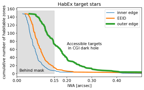
Figure 1: Cumulative number of HabEx target stars as a function of coronagraph IWA. The unobserved region obscured by the Roman Coronagraph HLC mask IWA is shaded. Systems in the unshaded reagion Roman can either access the habitable zone outer edge (top, thick green curve), earth-equivalent isolation distance (middle, orange curve) or the HZ inner edge (bottom, thin blue curve). The thick top curve corresponds to the young Mars edge while the bottom thin curve corresponds to the recent Venus inner edge. For this sample, 74 stars have at least a part of their HZ accessible, including 16 observable down to their EEID.

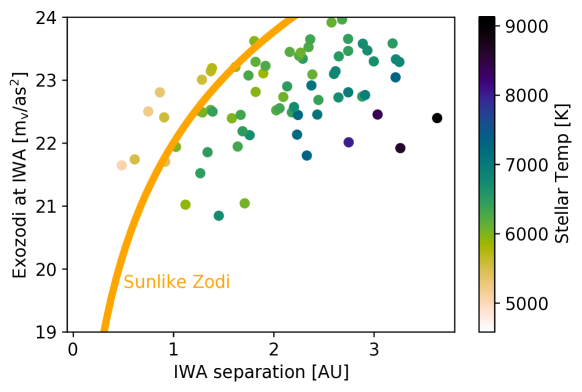
Figure 2: Target population surface brightness versus separation. The solid line shows the assumed surface brightness of a Solar-system-like exozodiacal as function of distance from the host star. Individual points show visible HZ’s surface brightness at the IWA and are colored by stellar temperature. Selection biases make the overall sample hotter than a Sunlike star.

Figure 3: Distribution of $5\sigma$ exozodi sensitivities for stars in the sample in the speckle limited, long exposure time, case. Narrow, dark bins correspond to evenly spaced bins; wide, lightly shaded bin sizes are set dynamically using the Bayesian Blocks method to show only significant differences in the distribution (Scargle et al., 2013). (a): current best-estimate median exozodiacal sensitivity where $\tilde{n_{Z}}$ is the calculated median number of zodi; (b): distribution of critical exozodi sensitivities for stars in the sample, for the “model uncertainty factor” (MUF) padded level of instrument performance, where the IWA increases to 0$\farcs$165 and the flux ratio sensitivity (contrast) degrades by a factor of two, the latter dominating the decrease in median sensitivity.

Geometry sets limits on the sample of HZ that Roman can observe at high-contrasts. Considering the exozodi around each star at the inner and outer edges of the HZ brackets the region of interest. While the surface brightness at the inner edge is greater, the outer edge is more likely to fall outside the IWA, leading to significantly more detections. This is seen in Figure 1, where the cumulative number of accessible habitable zones is shown as a function of coronagraphic inner working angle. The number of HZ outer edges (thick green line) inside the Coronagraph dark hole is 74 and eight inner edges (thin blue line) are visible, assuming the nominal 0$\farcs$15 IWA. Sixteen systems have an EEID inside the coronagraph dark hole (medium orange line). As stars get more distant, the coronagraph IWA translates to a larger physical separation that only remains within the HZ of the hottest and most luminous stars in the sample. This gradient in temperature is visible in Figure 2, which shows the surface brightness, the IWA separation in AU for each star with a visible HZ. The orange curve shows the surface brightness of the archetypal Solar zodiacal disk around a Sunlike star. Since there is a selection bias towards more luminous stars, the predicted exozodiacal surface brightness of the sample of geometrically observable HZ tends to be brighter than the solar zodiacal light at a given separation (see equation 1 with $M_{\star}>M_{\sun}$).

To quantify the exozodi sensitivity for each star in the sample, the critical sensitivity (Equation (6)) is calculated at the IWA for each star’s V-band magnitude and distance. Figure 3 shows a histogram of the number of stars observed as function of $n_{z}$, in the long exposure time limit. Because of the fixed IWA of the Roman coronagraph, the average star amenable to exozodi observations within the HZ is hotter than the Sun. And its exozodi surface brightness at a given physical separation is larger than expected around a Sun-like star (as shown in Figure 2). Since the irradiance received by the HZ is a constant by definition, these hotter stars have more widely separated HZ. increasing with stellar distance and since both density and irradiance are dropping the flux decreases $\propto d^{-\alpha}$, as shown in Equation (1). The long tail in Figure 3 above 60 zodi is made up of the four stars in the sample with the brightest apparent magnitude: Procyon, Altair, Fomalhaut, and Denebola. These stars have correspondingly higher speckle brightness relative to predicted exozodiacal dust surface brightness at the IWA, though they may be detectable at higher sensitivities if observed at larger separations. This is reflected by the spread of values in Figure 3 around the median value of $\sim$12 zodi, which does not include uncertainty in instrumental sensitivities.

To estimate the number of systems where exozodi may be detected at any level, we chose four representative values of $n_{z}$, unity (i.e. Solar) and the nominal median exozodi level, plus the $1\sigma$, and 95% confidence upper limits derived from the HOSTS survey (Ertel et al., 2020). (The $1\sigma$ HOSTS lower limit is zero). For each system on the target list, we drew increasing numbers of possible realizations of the log-normal distribution (with a standard deviation of $\varsigma=1.5$, the value found by Ertel et al. (2018b) for dust-less stars). The results stabilized after approximately 10,000 independent and identically distributed draws per case. The number of outer HZ exozodi which might be detectable for increasing values of $n_{z}$ are shown as half-“violin plots” in Figure 4. $n_{z}$ shown correspond to one zodi, the three zodi median from Ertel et al. (2020), as well as the 1$\sigma$ (nine zodi) and 95% confidence levels (27 zodi). Shaded regions’ widths indicate the underlying distribution, horizontal lines indicate the median and thin vertical lines represent 95% confidence intervals. Table 3 provides a summary of the same median exozodi levels with median and 95% confidence intervals. This assumed distribution is conservative, as will be discussed below.

Thus far, we have counted detections in the long exposure time regime. To estimate the minimum time for a survey, Equation (5) gives the exposure time as function of source flux, noise rate, and speckle rate. Applying this to our sample, Figure 5 shows the cumulative exposure time for the sample, given by Eq. 5, is hundreds of hours. The entire sample is likely observable to high SNR-per-resel in a few weeks time, albeit spread throughout the sidereal year and with additional observing overheads. Importantly, the second curve shown on Figure 5 demonstrates a much shorter exposure time is necessary to reach SNR =3 per resel, which will allow significant detection of extended disk structures quickly in multiple resels.

$n_{z}$	median	95% Confidence
27	51	43 - 58
9	31	23 - 39
3	13	7 - 20
1	4	1 - 8

Table 2: The number of systems that can be detected at a 5$\sigma$/resel cut-off, assuming infinite exposure time, a log-normal distribution, $\varsigma$=1.5 and median exozodi levels $n_{z}$, neglecting uncertainties in the instrument performance model.

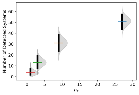
Figure 4: Expected number of systems with HZ exozodiacal dust detected by the Roman Coronagraph as a function of increasing median exozodi level ( $n_{z}$ in solar units). The y-axis represents $5\sigma$ exozodi detection for stars in the sample in speckle-limited case. The distributions of $5\sigma$ detections for the CBE sensitivity derived from randomly drawn log-normal distributions of increasing median-$n_{z}$ and $\varsigma$=1.5. Vertical bars represent the 95% percent confidence intervals, shaded regions show the underlying probability distributions, and horizontal bars indicate the median. For the HOSTS predicted median of 3 zodi, there is a $>95\%$ confidence that multiple systems will be detectable.

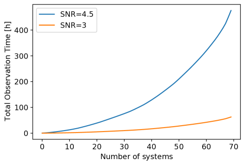
Figure 5: Number of observable systems versus cumulative mission exposure time, neglecting acquisition time or visibility, for the CBE sensitivity and detector properties. Each system is observed until the critical exozodi sensitivity is reached at $S=4.5$, since an SNR of five, by definition, is only reached at the critical dust level in an infinite exposure time. A 3$\sigma$ detection sensitivity exposure time is shown in the lower curve. A 3$\sigma$ detection in 3 resels, a likely scenario for most geometries, provides a $5\sigma$ detection of the presence of a disks around most stars in a significantly shorter survey.

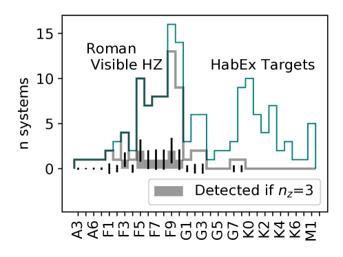
Figure 6: Histograms showing number of stars versus spectral type. Shaded region shows the median number of detected systems and bars indicated $1\sigma$ uncertainty calculated from the log-norm draws for the 3 zodi median case. The visible Roman HZ (medium width line) and the HabEx targets (thin line) peak at spectral type F9 but the Roman visible HZ go to zero at G8 and later-type. 95% of the HabEx targets (thin line) are FGK stars and all of the Roman predicted detections are FG stars.

4 Discussion

This analysis has shown the Roman Coronagraph will place new limits on scattered light brightness from exozodiacal dust in the HZ of nearby stars. Such a program would provide valuable insight into the scattered light background faced by future missions to image and spectrally characterize Earthlike planets. Simultaneously, such observations will increase our understanding of exozodiacal dynamical processes and constrain the relationship between IR observations of disk thermal emission and the light scattering albedo. As mentioned in Ertel et al. (2020), foreknowledge of which systems have excess exozodiacal light will allow better optimization of future direct imaging searches for Earthlike planets. Thus, both detections and upper limits on the brightness of scattered light at the CBE sensitivity decrease the uncertainty in both the median brightness and the brightness around specific stars. This has the potential to optimize the exoplanet observing strategy of future missions by allowing selective targeting of less dusty systems and, perhaps more importantly, informing the aperture required to detect Earthlike exoplanets and record their spectra at a useful SNR.

The results presented here retain the log-norm distribution as a conservative estimate of the Coronagraph exozodi detection rate, shown Figure 4. The 3 zodi distribution represents the median of the underlying exozodiacal brightness distribution reported by Ertel et al. (2020); however, the authors of that study found a log-norm distribution did not well fit the exozodiacal brightness function observed by HOSTS and instead chose to characterize the distribution with a free-form fit. HOSTS results show a subset of systems are dustier than the 3 zodi log-norm would predict, and hence may be easier to detect with the CBE performance of Coronagraph. HOSTS reported median $1\sigma$ sensitivity is 48 zodis for Sun-like stars and 23 zodis for early-type stars (A-F5). As seen in Fig. 6 the habitable zones visible to the Coronagaph straddle these two populations, largely made up of spectral types F5-G1, with the majority of the the exozodi detected in the 3 zodi log-normal case around stars F6 or redder. While the two populations studied are not identical, the CBE Roman median sensitivity (Figure 3(a)) is expected to be more than at least a factor of $\sim 2\times$ HOSTS and order of magnitude increase compared to HST Debes et al. (2019c).

As a technology demo, the minimum performance of the Roman Coronagraph is set by threshold requirements (Douglas et al., 2018) that are significantly more relaxed than the current-best-estimate sensitivity presented here. At threshold performance level, the IWA moves out to 0$\farcs$28, $t_{\rm occ}$ decreases to 0.05 and $\tau_{\ell}$ increases to 1.21E-9. Re-running the analysis above, while holding $f_{\Delta I}$ and $t_{\rm occ}^{\prime}$ constant, the $5\sigma$ exozodi sensitivity limit for the threshold mission sensitivity is of order $10,000$ zodi for 14 observable systems. This sensitivity to exozodiacal dust is implausibly low, since the increased photon rate would be expected to dramatically increase recovery of speckles and decrease $f_{\Delta I}$ from the assumed value. In this case, $f_{\Delta I}$ would approach the noiseless values of 0.01 to 0.05 (see appendix) but lacking detailed simulations of the instrument performance in the threshold performance regime we do not assert a predicted threshold performance sensitivity. Given the conservatism of the analytic estimates, on-orbit performance is expected to meet or exceed the CBE results presented, with the “model uncertainty” sensitivity of 25 zodi providing a likely lower limit. In particular, as shown in the appendix, when adding “model uncertainty” leakage the speckles are better attenuated, suggesting increased post-processing gain is a function of speckle brightness and brighter stars will also have brighter speckles for equal coronagraph performance. The median star in the Roman visible HZ sample is nearly 2$\times$ brighter than 47 Uma, suggesting additional post-processing gains may be achievable.

Future work is required to quantify the dependence of Coronagraph sensitivity to a range of higher order effects, including: morphological variation such as narrow rings or clumps (Defrère et al., 2010), partial transmission of light inside the IWA (Milani & Douglas, 2020), higher-order calibration and detector noise effects (Nemati, 2014), degeneracy between coronagraph leakage and disk morphology (particularly low-order aberrations), variations in composition and albedo (Debes et al., 2019a), sensitivity improvements from to matched filtering (Defrère et al., 2012), and dependence of post-processing gain on speckle lifetimes. Another phenomenon that the Coronagraph will be sensitive to is pseudo-zodi, where forward scattering from inclined asteroid belt analogs increases the background flux that appears close to the star (Stark et al., 2015a).

Mid-infrared observations, such as with Large Binocular Telescope Interferometer (LBTI) and including non-detections suggesting the dust is cool, will help disambiguate these cases. Currently, the Roman mission lifetime is fixed and the Coronagraph technology demonstration mission is currently planned for 3 months duration (Bailey et al., 2019). Detailed mission modeling will be required to establish the number of systems which can be observed in hypothetical Coronagraph observations following the technology demonstration phase.

Code to reproduce the figures presented in this study is available on github.com and archived on Zenodo (Douglas, 2020).

Simulated Disk Post-Processing: The speckle attenuation factor was derived from post-processing of the Roman-Coronagraph HLC Observing Scenario 9 data (OS9). This analysis used the HLC model with and without MUFs (margin of uncertainty factors). The processing procedure begins with photon counting both reference and target frames using the procedure outlined in Nemati (2020). To subtract the PSF we apply the NMF method of Ren et al. (2018) to construct PSF components from the OS9 reference frames. These were then subtracted from the target frames to arrive at a final processed frame. The ratio of the NMF-subtracted frames to the unprocessed frames near the IWA gives our speckle attenuation factor. To simulate cases with an edge-on disk Nemati’s EMCCD Detect code was used to simulate the response of an debris disk model (described in Mennesson et al. (2018) and publicly available) on Roman’s EMCCD. These were then added to each OS9 frame before the aforementioned photon counting procedure. The signal-to-noise ratio was computed by averaging the median per-pixel frame of the cases without disks for the processed and unprocessed cases separately These are shown in Figure 7. As a test of the NMF algorithm, an example inclined disk was inserted into the raw frames and is well recovered (bottom left).

Figure 8 shows the detector-noiseless and noisy speckle attenuation factor as the ratio of the radial average of the median speckle subtracted (NMF processed) image and the raw unprocessed speckle median image. Figure 8(b), the noisy curve shows the $f_{\Delta I}$ at the IWA is conservatively approximated by the assumed value of 0.25; equivalently, this is a post-processing gain of $4\times$.

The code to reproduce these figures is also available in the main publication repository (Douglas, 2020).

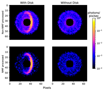
Figure 7: Comparison of the unprocessed (top) and processed (bottom) OS9 frames (without MUFs) with (left) and without (right) an inclined disk injected to demonstrate NMF’s ability to subtract speckles from the stellar PSF. Since self-subtraction is generally negligible for NMF post-processing, the speckle attenuation factor is given by taking the mean value of the ratio of the top right and bottom right images.

Figure 8: NMF post-processing speckle attenuation factor $f_{\Delta I}$, calculated as the ratio of the processed to unprocessed speckles as a function of radius for OS9 simulated observations of the 47 Uma system. The post-processing gain depends both on the temporal behavior of speckles at certain spatial frequencies and how well the speckles are resolved versus the noise floor. For the noiseless (a) only spatial frequency and sampling effects apply. When including detector and photon noise (b: coronagraph leakage is dominated by low-spatial frequencies, and speckles close to the IWA are better subtracted. Further from the star, detector noise begins to dominate and the attenuation factor flattens out. This simulation informed our choice of $f_{\Delta I}$ to be 0.25, a conservative approximation of the noisy simulation at 0$\farcs$15- 0$\farcs$20.

HIPPARCOS (ESA, 1997) identifiers of input catalog: 37279, 97649, 113368, 57632, 67927, 2021, 102422, 22449, 17378, 8102, 95501, 99240, 3821, 16537, 98036, 57757, 27072, 28103, 109176, 78072, 27321, 14632, 50954, 70497, 59199, 7513, 12777, 116771, 102485, 15510, 92043, 1599, 64394, 112447, 61317, 105858, 17651, 108870, 67153, 16852, 19849, 61174, 77257, 12843, 71284, 96100, 34834, 77760, 46509, 24813, 64924, 76829, 23693, 16245, 104214, 39903, 15457, 64408, 86486, 4151, 10644, 51459, 57443, 65721, 86736, 80686, 82860, 910, 47592, 5862, 109422, 73996, 29271, 53721, 25278, 97295, 48113, 95447, 88745, 86796, 7981, 29800, 25110, 97675, 40843, 45333, 104217, 64792, 3909, 15371, 56997, 114622, 32480, 47080, 49081, 80337, 73184, 84862, 78459, 12653, 18859, 58576, 32439, 89042, 79672, 22263, 8362, 15330, 7978, 99825, 3765, 35136, 107649, 12114, 38908, 42438, 105090, 81300, 75181, 98767, 26394, 3093, 49908, 84478, 43587, 3583, 23311, 56452, 72848, 40693, 13402, 100017, 114046, 54035, 27435, 544, 113283, 26779, 1475, 68184, 32984, 88972, 10798, 86400, 41926, 57939, 85235, 42808, 25878.

References

- Andrews et al. (2018) Andrews, S. M., Huang, J., Pérez, L. M., et al. 2018, ApJL, 869, L41, doi: 10.3847/2041-8213/aaf741
- Backman (1998) Backman, D. E. 1998, in Exozodiacal Dust Workshop (Moffett Field, Calif.; Springfield, VA: National Aeronautics and Space Administration, Ames Research Center ; Available from National Technical Information Service)
- Bailey et al. (2019) Bailey, V. P., Savransky, D., Debes, J., Mennesson, B., & Zellem, R. 2019, in Techniques and Instrumentation for Detection of Exoplanets IX, Vol. 11117 (International Society for Optics and Photonics), 111170E, doi: 10.1117/12.2527942
- Choquet et al. (2017) Choquet, É., Milli, J., Wahhaj, Z., et al. 2017, The Astrophysical Journal, 834, L12, doi: 10.3847/2041-8213/834/2/L12
- Currie et al. (2017) Currie, T., Guyon, O., Tamura, M., et al. 2017, ApJL, 836, L15, doi: 10.3847/2041-8213/836/1/L15
- Debes et al. (2019a) Debes, J., Choquet, E., Faramaz, V. C., et al. 2019a, arXiv:1906.02129 [astro-ph]. https://arxiv.org/abs/1906.02129
- Debes et al. (2019b) Debes, J. H., Ren, B., & Schneider, G. 2019b, JATIS, 5, 035003, doi: 10.1117/1.JATIS.5.3.035003
- Debes et al. (2019c) —. 2019c, arXiv:1905.06838 [astro-ph]. https://arxiv.org/abs/1905.06838
- Defrère et al. (2010) Defrère, D., Absil, O., den Hartog, R., Hanot, C., & Stark, C. 2010, A&A, 509, 9, doi: 10.1051/0004-6361/200912973;
- Defrère et al. (2012) Defrère, D., Stark, C., Cahoy, K., & Beerer, I. 2012, in Proc SPIE, ed. M. C. Clampin, G. G. Fazio, H. A. MacEwen, & J. M. Oschmann, Amsterdam, Netherlands, 84420M, doi: 10.1117/12.926324
- Defrère et al. (2015) Defrère, D., Hinz, P. M., Skemer, A. J., et al. 2015, The Astrophysical Journal, 799, 42, doi: 10.1088/0004-637X/799/1/42
- Dennihy et al. (2020) Dennihy, E., Farihi, J., Fusillo, N. P. G., & Debes, J. H. 2020, ApJ, 891, 97, doi: 10.3847/1538-4357/ab7249
- Douglas (2020) Douglas, E. 2020, doi: 10.5281/zenodo.4161937
- Douglas et al. (2018) Douglas, E. S., Carlton, A. K., Cahoy, K. L., et al. 2018, in Modeling, Systems Engineering, and Project Management for Astronomy VIII, Vol. 10705 (International Society for Optics and Photonics), 1070526, doi: 10.1117/12.2314221
- Douglas et al. (2020) Douglas, E. S., Ashcraft, J. N., Belikov, R., et al. 2020, in Space Telescopes and Instrumentation 2020: Optical, Infrared, and Millimeter Wave, Vol. 11443 (International Society for Optics and Photonics), 1144338, doi: 10.1117/12.2561960
- Duchene et al. (2020) Duchene, G., Rice, M., Hom, J., et al. 2020, AJ, 159, 251, doi: 10.3847/1538-3881/ab8881
- Ertel et al. (2018a) Ertel, S., Defrère, D., Hinz, P., et al. 2018a, AJ, 155, 194, doi: 10.3847/1538-3881/aab717
- Ertel et al. (2018b) Ertel, S., Kennedy, G. M., Defrère, D., et al. 2018b, 10698, 106981V, doi: 10.1117/12.2313685
- Ertel et al. (2020) Ertel, S., Defrère, D., Hinz, P., et al. 2020, AJ, 159, 177, doi: 10.3847/1538-3881/ab7817
- ESA (1997) ESA. 1997, 1200. http://adsabs.harvard.edu/abs/1997ESASP1200.....E
- Esposito et al. (2020) Esposito, T. M., Kalas, P., Fitzgerald, M. P., et al. 2020, AJ, 160, 24, doi: 10.3847/1538-3881/ab9199
- Gaidos (1998) Gaidos, E. J. 1998, ApJ, 510, L131, doi: 10.1086/311819
- Gaudi et al. (2020) Gaudi, B. S., Seager, S., Mennesson, B., et al. 2020, arXiv:2001.06683 [astro-ph]. https://arxiv.org/abs/2001.06683
- Ginsburg et al. (2018) Ginsburg, A., Sipocz, B., Parikh, M., et al. 2018, astropy/astroquery: v0.3.8 release, Zenodo, doi: 10.5281/zenodo.1234036
- Gustafson (1994) Gustafson, B. A. S. 1994, Annual Review of Earth and Planetary Sciences, 22, 553, doi: 10.1146/annurev.ea.22.050194.003005
- Hinz et al. (2004) Hinz, P. M., Connors, T., McMahon, T., et al. 2004, in Proc SPIE, Vol. 5491 (SPIE), 787–797, doi: 10.1117/12.552337
- Hughes et al. (2018) Hughes, A. M., Duchene, G., & Matthews, B. 2018, arXiv:1802.04313 [astro-ph]. https://arxiv.org/abs/1802.04313
- Hunter (2007) Hunter, J. D. 2007, Computing In Science & Engineering, 9, 90, doi: 10.1109/MCSE.2007.55
- Jones et al. (2001) Jones, E., Oliphant, T., & Peterson, P. 2001, http://www. scipy. org/. http://www.citeulike.org/group/2018/article/2644428
- Kalas et al. (2005) Kalas, P., Graham, J. R., & Clampin, M. 2005, Nature, 435, 1067, doi: 10.1038/nature03601
- Kaltenegger (2017) Kaltenegger, L. 2017, Annual Review of Astronomy and Astrophysics, 55, 433, doi: 10.1146/annurev-astro-082214-122238
- Kasdin et al. (2018) Kasdin, N. J., Turnbull, M., Macintosh, B., et al. 2018, in Space Telescopes and Instrumentation 2018: Optical, Infrared, and Millimeter Wave, Vol. 10698 (International Society for Optics and Photonics), 106982H, doi: 10.1117/12.2315002
- Kasting et al. (1993) Kasting, J. F., Whitmire, D. P., & Reynolds, R. T. 1993, Icarus, 101, 108, doi: 10.1006/icar.1993.1010
- Kelsall et al. (1998) Kelsall, T., Weiland, J. L., Franz, B. A., et al. 1998, ApJ, 508, 44, doi: 10.1086/306380
- Kennedy et al. (2015) Kennedy, G. M., Wyatt, M. C., Bailey, V., et al. 2015, ApJS, 216, 23, doi: 10.1088/0067-0049/216/2/23
- Kluyver et al. (2016) Kluyver, T., Ragan-Kelley, B., Pérez, F., et al. 2016, in Positioning and Power in Academic Publishing: Players, Agents and Agendas, 87–90, doi: 10.3233/978-1-61499-649-1-87
- Kopparapu et al. (2013) Kopparapu, R., Ramirez, R., Kasting, J. F., et al. 2013, ApJ, 765, 131, doi: 10.1088/0004-637X/765/2/131
- Kral et al. (2017) Kral, Q., Krivov, A. V., Defrère, D., et al. 2017, Astronomical Review, 0, 1, doi: 10.1080/21672857.2017.1353202
- Krist et al. (2017) Krist, J., Riggs, A. J., McGuire, J., et al. 2017, in Techniques and Instrumentation for Detection of Exoplanets VIII, Vol. 10400 (International Society for Optics and Photonics), 1040004, doi: 10.1117/12.2274792
- Krist et al. (2018) Krist, J., Effinger, R., Kern, B., et al. 2018, in Space Telescopes and Instrumentation 2018: Optical, Infrared, and Millimeter Wave, Vol. 10698 (International Society for Optics and Photonics), 106982K, doi: 10.1117/12.2310043
- Krist (2004) Krist, J. E. 2004, in Proc. SPIE, Vol. 5487, 1284–1295, doi: 10.1117/12.548890
- Krist (2007) Krist, J. E. 2007, in Proc. SPIE, Vol. 6675, 66750P–66750P–9, doi: 10.1117/12.731179
- Krist (2014) Krist, J. E. 2014, in Proc. SPIE, Vol. 9143, 91430V–91430V–16, doi: 10.1117/12.2056759
- Krist et al. (2015) Krist, J. E., Nemati, B., & Mennesson, B. P. 2015, JATIS, 2, 011003, doi: 10.1117/1.JATIS.2.1.011003
- Krist et al. (2012) Krist, J. E., Stapelfeldt, K. R., Bryden, G., & Plavchan, P. 2012, The Astronomical Journal, 144, 45, doi: 10.1088/0004-6256/144/2/45
- Lacy & Burrows (2020) Lacy, B., & Burrows, A. 2020, ApJ, 892, 151, doi: 10.3847/1538-4357/ab7017
- Lafrenière et al. (2009) Lafrenière, D., Marois, C., Doyon, R., & Barman, T. 2009, The Astrophysical Journal, 694, L148, doi: 10.1088/0004-637X/694/2/L148
- Lafrenière et al. (2007) Lafrenière, D., Marois, C., Doyon, R., Nadeau, D., & Artigau, É. 2007, ApJ, 660, 770, doi: 10.1086/513180
- Lawrence (1992) Lawrence, G. N. 1992, in Applied Optics and Optical Engineering., ed. R. R. Shannon & J. C. Wyant., Vol. XI (New York: Academic Press)
- Lupu et al. (2016) Lupu, R. E., Marley, M. S., Lewis, N., et al. 2016, The Astronomical Journal, 152, 217, doi: 10.3847/0004-6256/152/6/217
- MacGregor et al. (2016) MacGregor, M. A., Lawler, S. M., Wilner, D. J., et al. 2016, ApJ, 828, 113, doi: 10.3847/0004-637X/828/2/113
- Males et al. (2015) Males, J. R., Belikov, R., & Bendek, E. 2015, arXiv:1510.02478 [astro-ph], 960518, doi: 10.1117/12.2188766
- Mennesson et al. (2014) Mennesson, B., Millan-Gabet, R., Serabyn, E., et al. 2014, ApJ, 797, 119, doi: 10.1088/0004-637X/797/2/119
- Mennesson et al. (2018) Mennesson, B., Kasdin, N. J., Macintosh, B., et al. 2018, in Space Telescopes and Instrumentation 2018: Optical, Infrared, and Millimeter Wave, ed. H. A. MacEwen, M. Lystrup, G. G. Fazio, N. Batalha, E. C. Tong, & N. Siegler (Austin, United States: SPIE), 88, doi: 10.1117/12.2313861
- Mennesson et al. (2020) Mennesson, B., Juanola-Parramon, R., Nemati, B., et al. 2020, arXiv:2008.05624 [astro-ph]. https://arxiv.org/abs/2008.05624
- Mennesson et al. (2021) Mennesson, B., Bailey, V. P., Zellem, R., et al. 2021, in Techniques and Instrumentation for Detection of Exoplanets X, Vol. 11823 (SPIE), 335–346, doi: 10.1117/12.2603343
- Milani & Douglas (2020) Milani, K., & Douglas, E. S. 2020, in Optical Modeling and Performance Predictions XI, Vol. 11484 (International Society for Optics and Photonics), 1148405, doi: 10.1117/12.2568204
- Nemati (2014) Nemati, B. 2014, in Space Telescopes and Instrumentation 2014: Optical, Infrared, and Millimeter Wave, Vol. 9143 (International Society for Optics and Photonics), 91430Q, doi: 10.1117/12.2060321
- Nemati (2020) Nemati, B. 2020, in Space Telescopes and Instrumentation 2020: Optical, Infrared, and Millimeter Wave, ed. M. Lystrup, M. D. Perrin, N. Batalha, N. Siegler, & E. C. Tong, Vol. 11443, International Society for Optics and Photonics (SPIE), 884 – 895. https://doi.org/10.1117/12.2575983
- Nemati et al. (2017) Nemati, B., Krist, J. E., & Mennesson, B. 2017, in Techniques and Instrumentation for Detection of Exoplanets VIII, Vol. 10400 (International Society for Optics and Photonics), 1040007, doi: 10.1117/12.2274396
- Nemati et al. (2020) Nemati, B., Stahl, H. P., Stahl, M. T., Ruane, G. J. J., & Sheldon, L. J. 2020, JATIS, 6, 039002, doi: 10.1117/1.JATIS.6.3.039002
- Nesvorný et al. (2010) Nesvorný, D., Jenniskens, P., Levison, H. F., et al. 2010, ApJ, 713, 816, doi: 10.1088/0004-637X/713/2/816
- Patel et al. (2014) Patel, R. I., Metchev, S. A., & Heinze, A. 2014, ApJS, 212, 10, doi: 10.1088/0067-0049/212/1/10
- Pérez & Granger (2007) Pérez, F., & Granger, B. 2007, Computing in Science Engineering, 9, 21, doi: 10.1109/MCSE.2007.53
- Perrin et al. (2015) Perrin, M. D., Duchene, G., Millar-Blanchaer, M., et al. 2015, ApJ, 799, 182, doi: 10.1088/0004-637X/799/2/182
- Poberezhskiy et al. (2021) Poberezhskiy, I., Luchik, T., Zhao, F., et al. 2021, in Space Telescopes and Instrumentation 2020: Optical, Infrared, and Millimeter Wave, Vol. 11443 (International Society for Optics and Photonics), 114431V, doi: 10.1117/12.2563480
- Ramirez & Kaltenegger (2016) Ramirez, R. M., & Kaltenegger, L. 2016, ApJ, 823, 6, doi: 10.3847/0004-637X/823/1/6
- Ren (2020) Ren, B. 2020, nmf_imaging: Second Release, Zenodo, doi: 10.5281/zenodo.3738623
- Ren et al. (2017) Ren, B., Pueyo, L., Perrin, M. D., Debes, J. H., & Choquet, É. 2017, in Techniques and Instrumentation for Detection of Exoplanets VIII, Vol. 10400 (International Society for Optics and Photonics), 1040021, doi: 10.1117/12.2274163
- Ren et al. (2018) Ren, B., Pueyo, L., Zhu, G. B., Debes, J., & Duchêne, G. 2018, ApJ, 852, 104, doi: 10.3847/1538-4357/aaa1f2
- Riggs et al. (2021) Riggs, A. J. E., Moody, D., Gersh-Range, J., et al. 2021, Techniques and Instrumentation for Detection of Exoplanets X, 72, doi: 10.1117/12.2598599
- Roberge et al. (2012) Roberge, A., Chen, C. H., Millan-Gabet, R., et al. 2012, PASP, 124, 799, doi: 10.1086/667218
- Rodigas et al. (2012) Rodigas, T. J., Hinz, P. M., Leisenring, J., et al. 2012, ApJ, 752, 57, doi: 10.1088/0004-637X/752/1/57
- Rodigas et al. (2016) Rodigas, T. J., Arriagada, P., Faherty, J., et al. 2016, ApJ, 818, 106, doi: 10.3847/0004-637X/818/2/106
- Savransky et al. (2017) Savransky, D., Delacroix, C., & Garrett, D. 2017, Astrophysics Source Code Library, ascl:1706.010. http://adsabs.harvard.edu/abs/2017ascl.soft06010S
- Savransky & Garrett (2016) Savransky, D., & Garrett, D. 2016, Journal of Astronomical Telescopes, Instruments, and Systems, 2, 011006, doi: 10.1117/1.JATIS.2.1.011006
- Savransky et al. (2009) Savransky, D., Kasdin, N. J., & Cady, E. 2009, arXiv:0903.4915, doi: 10.1086/652181
- Scargle et al. (2013) Scargle, J. D., Norris, J. P., Jackson, B., & Chiang, J. 2013, The Astrophysical Journal, 764, 167, doi: 10.1088/0004-637X/764/2/167
- Schmid et al. (2018) Schmid, H. M., Bazzon, A., Roelfsema, R., et al. 2018, A&A, 619, A9, doi: 10.1051/0004-6361/201833620
- Schneider (2014) Schneider, G. 2014, arXiv:1412.8421 [astro-ph]. https://arxiv.org/abs/1412.8421
- Schneider et al. (2014) Schneider, G., Grady, C. A., Hines, D. C., et al. 2014, The Astronomical Journal, 148, 59, doi: 10.1088/0004-6256/148/4/59
- Schwieterman et al. (2018) Schwieterman, E. W., Kiang, N. Y., Parenteau, M. N., et al. 2018, Astrobiology, 18, 663, doi: 10.1089/ast.2017.1729
- Seager (2013) Seager, S. 2013, Science, 340, 577, doi: 10.1126/science.1232226
- Shi et al. (2016) Shi, F., Balasubramanian, K., Bartos, R., et al. 2016, in Proc. SPIE, 990418, doi: 10.1117/12.2234226
- Shields et al. (2016) Shields, A. L., Ballard, S., & Johnson, J. A. 2016, Physics Reports, 663, 1, doi: 10.1016/j.physrep.2016.10.003
- Silverberg et al. (2018) Silverberg, S. M., Kuchner, M. J., Wisniewski, J. P., et al. 2018, ApJ, 868, 43, doi: 10.3847/1538-4357/aae3e3
- Smith et al. (2018) Smith, J. S., Bartusek, L., Casey, T., et al. 2018, in Space Telescopes and Instrumentation 2018: Optical, Infrared, and Millimeter Wave, Vol. 10698 (SPIE), 745–754, doi: 10.1117/12.2311772
- Soummer et al. (2012) Soummer, R., Pueyo, L., & Larkin, J. 2012, ApJ, 755, L28, doi: 10.1088/2041-8205/755/2/L28
- Stark & Kuchner (2008) Stark, C. C., & Kuchner, M. J. 2008, ApJ, 686, 637, doi: 10.1086/591442
- Stark et al. (2015a) Stark, C. C., Kuchner, M. J., & Lincowski, A. 2015a, ApJ, 801, 128, doi: 10.1088/0004-637X/801/2/128
- Stark et al. (2015b) Stark, C. C., Roberge, A., Mandell, A., et al. 2015b, The Astrophysical Journal, 808, 149, doi: 10.1088/0004-637X/808/2/149
- Stark et al. (2014) Stark, C. C., Roberge, A., Mandell, A., & Robinson, T. D. 2014, ApJ, 795, 122, doi: 10.1088/0004-637X/795/2/122
- Stark et al. (2016) Stark, C. C., Cady, E. J., Clampin, M., et al. 2016, in Proc SPIE, Vol. 9904, 99041U–99041U–13, doi: 10.1117/12.2233201
- Szalay et al. (2020) Szalay, J. R., Pokorný, P., Bale, S. D., et al. 2020, ApJS, 246, 27, doi: 10.3847/1538-4365/ab50c1
- Team (2019) Team, T. L. 2019, arXiv:1912.06219 [astro-ph]. https://arxiv.org/abs/1912.06219
- The Astropy Collaboration et al. (2013) The Astropy Collaboration, Robitaille, T. P., Tollerud, E. J., et al. 2013, Astronomy & Astrophysics, 558, A33, doi: 10.1051/0004-6361/201322068
- Trauger et al. (2016) Trauger, J., Moody, D., Krist, J., & Gordon, B. 2016, J. Astron. Telesc. Instrum. Syst, 2, 011013, doi: 10.1117/1.JATIS.2.1.011013
- Turnbull et al. (2012) Turnbull, M. C., Glassman, T., Roberge, A., et al. 2012, PASP, 124, 418. http://iopscience.iop.org/article/10.1086/666325/meta
- Wright et al. (2010) Wright, E. L., Eisenhardt, P. R. M., Mainzer, A. K., et al. 2010, The Astronomical Journal, 140, 1868, doi: 10.1088/0004-6256/140/6/1868
- Wyatt (2005) Wyatt, M. C. 2005, A&A, 433, 1007, doi: 10.1051/0004-6361:20042073
- Wyatt (2008) —. 2008, Annual Review of Astronomy and Astrophysics, 46, 339, doi: 10.1146/annurev.astro.45.051806.110525
- Ygouf et al. (2021) Ygouf, M., Zimmerman, N., Bailey, V., et al. 2021, Roman Coronagraph Instrument Post Processing Report - OS9 HLC Distribution, Tech. rep., IPAC, Pasadena, California, USA. https://wfirst.ipac.caltech.edu/docs/sims/20210402_Roman_CGI_post_processing_report_URS.pdf
- Ygouf et al. (2016) Ygouf, M., Zimmerman, N. T., Pueyo, L., et al. 2016, in Space Telescopes and Instrumentation 2016: Optical, Infrared, and Millimeter Wave, Vol. 9904 (International Society for Optics and Photonics), 99045M, doi: 10.1117/12.2231581
- Young et al. (2013) Young, E. J., Kasdin, N. J., & Carlotti, A. 2013, in Proc. SPIE, Vol. 8864, 88640S–88640S–13, doi: 10.1117/12.2025061
- Zhou et al. (2018) Zhou, H., Krist, J., Cady, E., & Poberezhskiy, I. 2018, in Space Telescopes and Instrumentation 2018: Optical, Infrared, and Millimeter Wave, Vol. 10698 (International Society for Optics and Photonics), 106982M, doi: 10.1117/12.2313719
- Zhou et al. (2020) Zhou, H., Krist, J., Seo, B.-J., et al. 2020, in Space Telescopes and Instrumentation 2020: Optical, Infrared, and Millimeter Wave, Vol. 11443 (SPIE), 314–323, doi: 10.1117/12.2561087
- Zhu (2016) Zhu, G. 2016, Nonnegative Matrix Factorization (NMF) with Heteroscedastic Uncertainties and Missing data. https://ui.adsabs.harvard.edu/abs/2016arXiv161206037Z