Existence, Stability and Dynamics of Monopole and
Alice Ring Solutions in Anti-Ferromagnetic Spinor Condensates

Abstract

In this work we study the existence, stability, and dynamics of select topological point and line defects in anti-ferromagnetic, polar phase, $F=1$ ²³Na spinor condensates. Specifically, we leverage fixed-point and numerical continuation techniques in three spatial dimensions to identify solution families of monopole and Alice rings as the chemical potential (number of atoms) and trapping strengths are varied within intervals of realizable experimental parameters. We are able to follow the monopole from the linear limit of small atom number all the way to the Thomas-Fermi regime of large atom number. Additionally, and importantly, our studies reveal the existence of two Alice ring solution branches, corresponding to, relatively, smaller and larger ring radii, that bifurcate from each other in a saddle-center bifurcation as the chemical potential is varied. We find that the monopole solution is always dynamically unstable in the regimes considered. In contrast, we find that the larger Alice ring is indeed stable close to the bifurcation point until it destabilizes from an oscillatory instability bubble for a larger value of the chemical potential. We also report on the possibility of dramatically reducing, yet not completely eliminating, the instability rates for the smaller Alice ring by varying the trapping strengths. The dynamical evolution of the different unstable waveforms is also probed via direct numerical simulations.

I Introduction

The study of Bose-Einstein condensates (BECs) is a topic that has now enjoyed two and a half decades of substantial renewed interest given the experimental (and theoretical) developments in the field that have now been succinctly summarized in a number of books Pethick and Smith (2008); Pitaevskii and Stringari (2018). While the simplest scenario of such BECs has involved single-component/single-species atomic gases, it was quickly realized that the internal degrees of freedom of, e.g., different hyperfine states or the condensation of multiple gases could offer a significant laboratory of novel physical phenomena including phase separation, spin dynamics, and domain walls, among many others Stamper-Kurn et al. (1998); Stenger et al. (1998); Stamper-Kurn et al. (1999); Chang et al. (2005); Widera et al. (2006). Such multi-component systems are often studied in the realm of so-called spinor condensates corresponding to hyperfine states of $F=1$ and $F=2$ and, as such, have been the subject of numerous dedicated reviews Kawaguchi and Ueda (2012); Stamper-Kurn and Ueda (2013); Kevrekidis and Frantzeskakis (2016), as well as of books Pethick and Smith (2008); Pitaevskii and Stringari (2018); Kevrekidis et al. (2015).

A key feature of spinor condensates is the presence of both spin-independent and spin-dependent interactions Kawaguchi and Ueda (2012); Stamper-Kurn and Ueda (2013). Depending on the sign of the latter, the gases can be anti-ferromagnetic, as in the case of ²³Na Stamper-Kurn et al. (1998); Stenger et al. (1998) or ferromagnetic (weakly or strongly, respectively) for ⁸⁷Rb Chang et al. (2005); Widera et al. (2006) and ⁷Li Huh et al. (2020); Kim et al. (2021). The phase diagram of the potential ground states (depending on the spin-dependent interactions and the role of external magnetic fields through the so-called quadratic Zeeman effect) has been extensively studied, e.g., in Ref. Kawaguchi and Ueda (2012).

Beyond such ground states, part of the wealth of the phenomenology enabled by the 3-component $F=1$ and the 5-component $F=2$ BECs concerns the possibility of solitonic (both topological and non-topological) excitations in them Kevrekidis et al. (2015). Indeed, at the one-dimensional (1D) level, both magnetic and non-magnetic structures have been theoretically proposed and experimentally observed Li et al. (2005); Zhang et al. (2007); Nistazakis et al. (2008); Szankowski et al. (2011); Romero-Ros et al. (2019); Chai et al. (2020, 2021); Bersano et al. (2018); Fujimoto et al. (2019) whence the phase diagram Katsimiga et al. (2021), as well as multi-soliton collisions Lannig et al. (2020) of some of these structures have been theoretically explored and experimentally quantified. The presence of the spin degree of freedom has also enabled the observation of spin domains Miesner et al. (1999); Świsłocki and Matuszewski (2012) and spin textures Ohmi and Machida (1998a); Song et al. (2013). Although there are numerous topological and vortical structures that have been uncovered in this setting Al Khawaja and Stoof (2001); Mizushima et al. (2002a); Reijnders et al. (2004); Mizushima et al. (2002b); Leslie et al. (2009), including even quantum knots Hall et al. (2016); Lee et al. (2018), our focus herein will be on the existence, stability and dynamical properties of elusive structures that have recently found a fertile ground for their creation in this spinor setting, namely monopoles Stoof et al. (2001); Ray et al. (2015); Ollikainen et al. (2017) and Alice rings Ruostekoski and Anglin (2003).

To that end, we will first explore the monopole structure from a dynamical systems point of view. Initially, we will explore its existence, showcasing how it can be started in a three-dimensional (3D) parabolic confinement setting from the near-linear, low-atom-number limit, and continued towards the large-atom-number, nonlinear (so-called Thomas-Fermi) regime. We will subsequently develop stability diagnostics for this 3D spatial structure as an equilibrium state and identify the modes that render it unstable. The evolution of such an instability will offer a hint towards the existence of a symmetry-broken state, in the form of the so-called Alice ring (AR) Ruostekoski and Anglin (2003); Tiurev et al. (2016). The latter state comes in two variants (with a smaller and a larger ring, respectively) which terminate, via a saddle-center bifurcation, at the same turning point, i.e., at a minimal value of the chemical potential for which such solutions can exist. The stability and dynamics of such ARs are examined as well.

Our presentation is structured as follows. In Sec. II, we present the general setup of the spinor model and discuss its main properties. In Sec. III, we present the features of the monopole solution, while in Sec. IV, an analogous presentation is put forth for the AR. Finally, in Sec. V, we summarize our findings and present some conclusions, as well as a number of directions for future work.

II Preliminaries

II.1 Model

The energy functional for the three spin-states wavefunction $\Psi=(\psi_{+1},\psi_{0},\psi_{-1})$ of the $F=1$ spinor condensate Kawaguchi and Ueda (2012); Robins et al. (2001) is given by

$$\mathcal{E}=\iiint_{-\infty}^{+\infty}d\mathbf{r}\Big{\{}\sum_{m=-1}^{1}\psi_{m}^{\ast}\hat{h}_{0}\psi_{m}+\frac{g_{0}}{2}n^{2}+\frac{g_{2}}{2}|\mathbf{F}|^{2}\Big{\}},$$ (1)

where the linear operator $\hat{h}_{0}=-\frac{\hbar^{2}}{2M}\nabla^{2}+V$ accounts for the kinetic energy with $V=V(\textbf{r})$ corresponding to the external trapping potential for atoms of mass $M$. The total density is defined as

$$n=n_{-1}+n_{0}+n_{+1}=\sum_{m=-1}^{1}|\psi_{m}|^{2},$$ (2)

and the scattering coefficients are given by $g_{0}={4\pi\hbar^{2}a_{s}}/{m}$ and $g_{2}={4\pi\hbar^{2}a_{a}}/{m}$ where $a_{s}$ and $a_{a}$ characterize, respectively, the spin-independent and spin-dependent part of the interactions. In particular, $a_{s}=(2a_{2}+a_{0})/3$ and $a_{a}=(a_{2}-a_{0})/3$ Kawaguchi and Ueda (2012); Ohmi and Machida (1998b); Ho (1998) with the values of $a_{0}$ and $a_{2}$ given in Table 2 of Ref. Kawaguchi and Ueda (2012). The spin density vector $\mathbf{F}=(F_{x},F_{y},F_{z})$ is given by

$$F_{a}=\sum_{m,n=-1}^{1}\psi_{m}^{\ast}(f_{a})_{mn}\psi_{n},\quad a\in\{x,y,z\},$$ (3)

where $f_{a}$ represent the Pauli’s spin-1 matrices. The components of the spin (magnetization) vector $\mathbf{F}$ are

$$F_{x} = \frac{1}{\sqrt{2}}[\psi_{+1}^{\ast}\psi_{0}+\psi_{0}^{\ast}(\psi_{+1}+\psi_{-1})+\psi^{\ast}_{-1}\psi_{0}],$$

$$F_{y} = \frac{i}{\sqrt{2}}[-\psi_{+1}^{\ast}\psi_{0}+\psi_{0}^{\ast}(\psi_{+1}-\psi_{-1})+\psi^{\ast}_{-1}\psi_{0}],$$

$$F_{z} = |\psi_{+1}|^{2}-|\psi_{-1}|^{2}.$$

For the $F=1$ spinor condensate, the mean-field order parameter $\Psi$ can be expressed as $\Psi(\mathbf{r})=\sqrt{n}e^{i\phi}\zeta(\mathbf{r})$, where $\phi(\mathbf{r})$ is the scalar global phase and $\zeta(\mathbf{r})$ represents the normalized spinor which determines the average local spin $\langle\mathbf{F}\rangle=\mathbf{\zeta}^{\dagger}\mathbf{F}\mathbf{\zeta}$ Stoof et al. (2001); Stamper-Kurn and Ueda (2013). The equations of motion for $\Psi$ ensuing from the energy functional of Eq. (1) correspond to the following set of spin-coupled Gross-Pitaevskii (GP) equations:

$$i\hbar\frac{\partial\psi_{+1}}{\partial t} =\mathcal{H}\psi_{+1}+g_{2}(|\psi_{0}|^{2}+F_{z})\psi_{+1}+g_{2}\psi_{-1}^{\ast}\psi_{0}^{2},$$ (4a)

$$i\hbar\frac{\partial\psi_{0}}{\partial t} =\mathcal{H}\psi_{0}+g_{2}(|\psi_{+1}|^{2}+|\psi_{-1}|^{2})\psi_{0}+2g_{2}\psi_{0}^{\ast}\psi_{+1}\psi_{-1},$$ (4b)

$$i\hbar\frac{\partial\psi_{-1}}{\partial t} =\mathcal{H}\psi_{-1}+g_{2}(|\psi_{0}|^{2}-F_{z})\psi_{-1}+g_{2}\psi_{+1}^{\ast}\psi_{0}^{2},$$ (4c)

where

$$\mathcal{H}=\hat{h}_{0}+g_{0}\,n,$$

represents the spin-independent nonlinear operator, arising in the famous Manakov model Manakov (1974). The external potential in Eq. (4) is assumed to be the same for all spin components, and is given by

$$V(\textbf{r})=\frac{1}{2}m\left(\Omega_{x}^{2}x^{2}+\Omega_{y}^{2}y^{2}+\Omega_{z}^{2}z^{2}\right),$$

where $\Omega_{a}$ is the trapping strength along the $a$th direction. Note that we allow the parabolic trap to have independent strengths along all spatial directions as we are also interested in studying the effects on the existence and possible stabilization of the topological structures at hand, namely monopoles and Alice rings (ARs), when introducing, relatively weak, in-plane $(x,y)$ anisotropies.

The spinor condensate admits multiple conserved quantities Kawaguchi and Ueda (2012). These are (i) the total atom number

$$\mathcal{N}=\mathcal{N}_{-1}+\mathcal{N}_{0}+\mathcal{N}_{+1},$$ (5)

corresponding to the sum of all atom numbers for each component (which are not individually conserved):

$$\mathcal{N}_{j}=\iiint_{-\infty}^{+\infty}|\psi_{j}|^{2}\,dx\,dy\,dz,\quad j\in\{-1,0,+1\},$$ (6)

(ii) the $z$-component of the magnetization

$$\mathcal{M}_{z}=\iiint_{-\infty}^{+\infty}F_{z}\,dx\,dy\,dz,$$

and (iii) the integral of the modulus squared of the magnetization (spin) vector, in addition to (iv) the energy of Eq. (1) which represents the Hamiltonian of the model.

For the simulations, we will resort to the dimensionless version of the GP equations [cf. Eqs. (4)] by initially assuming a spherical trap with $\Omega\equiv\Omega_{x}=\Omega_{y}=\Omega_{z}$ and using the rescalings $x\rightarrow a_{0}x$, $t\rightarrow\Omega^{-1}t$, and $\psi_{j}\rightarrow\sqrt{N}a_{0}^{-3/2}\psi_{j}$ where $a_{h}=\sqrt{\frac{\hbar}{M\Omega}}$ is the harmonic oscillator length. Note that, for ease of exposition, we keep the same notation as the dimensional variables. However, from this point onwards it is important to remember that all variables are dimensionless. Under this adimensionalization, the GP equations become

$$\begin{split}\small i\frac{\partial\psi_{+1}}{\partial t}&=\mathcal{H}\psi_{+1}+c_{2}(|\psi_{0}|^{2}+F_{z})\psi_{+1}+c_{2}\psi_{-1}^{\ast}\psi_{0}^{2},\\ \small i\frac{\partial\psi_{0}}{\partial t}&=\mathcal{H}\psi_{0}+c_{2}(|\psi_{+1}|^{2}+|\psi_{-1}|^{2})\psi_{0}+2c_{2}\psi_{0}^{\ast}\psi_{+1}\psi_{-1},\\ \small i\frac{\partial\psi_{-1}}{\partial t}&=\mathcal{H}\psi_{-1}+c_{2}(|\psi_{0}|^{2}-F_{z})\psi_{-1}+c_{2}\psi_{+1}^{\ast}\psi_{0}^{2},\end{split}$$ (7)

where

$$\mathcal{H} = -\frac{1}{2}\nabla^{2}+V(\textbf{r})+c_{0}\,n,$$ (8)

$$V(\textbf{r}) = \frac{1}{2}(x^{2}+y^{2}+z^{2}),$$ (9)

and $c_{0}=4\pi Na_{s}/a_{h}$, while $c_{2}=4\pi Na_{a}/a_{h}$. Typically, $a_{h}/a_{s}$ varies between 500 and 4000 Leanhardt et al. (2003); Ruostekoski and Anglin (2003). Following Refs. Stenger et al. (1998); Black et al. (2007); Samuelis et al. (2000), we consider, in particular, a ²³Na condensate with $a_{a}=(a_{2}-a_{0})/3\approx 2a_{B}$ and $a_{s}=(2a_{2}+a_{0})/3\approx 50a_{B}$ in our simulations where $a_{B}=0.0529\,$nm is the Bohr radius, thus giving $c_{2}/c_{0}\approx 0.04$. For instance, for trapping frequencies $\Omega=2\pi\times 10\,$Hz and and $N\approx 4\times 10^{6}$, we get $c_{0}=2\times 10^{4}$.

II.2 Ground State Phases

In the absence of magnetic field (Zeeman terms), the ground state can be either (i) ferromagnetic (${\cal M}_{z}\neq 0$ and $c_{2}<0$) or (ii) anti-ferromagnetic or polar (${\cal M}_{z}=0$ and $c_{2}>0$) Kawaguchi and Ueda (2012). In the present work, we focus on the polar case where the order parameter is $(0,1,0)^{T}$, i.e., the hyperfine state corresponding to $m_{f}=0$ is the only one populated at the ground state. For a $F=1$ spinor condensate, the mass velocity acquires the form

$$\mathbf{v}^{\rm mass}=\frac{\hbar}{M}(\nabla\phi-i\mathbf{\zeta}^{\dagger}\nabla\mathbf{\zeta}).$$ (10)

Nevertheless, the absence of magnetization in the polar phase simplifies the mass velocity to $\mathbf{v}^{\rm mass}=\left(\hbar/M\right)\nabla\phi$. As a result, mass circulation along a loop is quantized; yet, the single-valuedness of the order parameter, $\Psi$, demands the quantization of circulation in units of $h/(2M)$ (half-quantum vortex) Kawaguchi and Ueda (2012). This stems from the fact that for ${\cal M}_{z}=0$, the order parameter $\Psi$ can be represented as

$$\Psi=\sqrt{n}e^{i\phi}\hat{\mathbf{d}},$$ (11)

where $\hat{\mathbf{d}}$ is a unit vector that defines the quantization axis, and that would yield ($\hat{\mathbf{d}},\phi)\rightarrow(-\hat{\mathbf{d}},\phi+\pi)$. This invariance reflects the $\mathbb{Z}_{2}$ symmetry of $\Psi$.

III Monopole

A monopole is a topologically excited point defect and is characterized by the second homotopy group ($\pi_{2}$) Kawaguchi and Ueda (2012). It can be realized in a BEC either by breaking the global symmetry of the condensate or by a gauge-potential Pietilä and Möttönen (2009); Kawaguchi and Ueda (2012). These structures can be naturally realized in a spinor condensate. Indeed, since in the polar phase of the $F=1$ spinor condensate we are free to change the (global) phase and spin, a monopole can be created by choosing the (radial) hedgehog field $\hat{\mathbf{d}}={\mathbf{r}}/{r}$ (where $r=|\mathbf{r}|$) in Eq. (11) with $\phi=0$ by minimizing the gradient energy Ruostekoski and Anglin (2003); Stoof et al. (2001). Such a monopole is called ’t-Hooft-Polyakov monopole Ruostekoski and Anglin (2003). The $\psi_{\pm 1}$ components in the case of such a monopole feature overlapped vortex lines each carrying a single quantum of angular momentum (but opposite circulation between the two). On the other hand, $\psi_{0}$ resembles a planar dark soliton (i.e., featuring a $\pi$-phase jump across the soliton plane) as indicated in Ref. Ruostekoski and Anglin (2003). Moreover, for a monopole, Eq. (11) vanishes at the origin, i.e., the density $n(\mathbf{0})=0$.

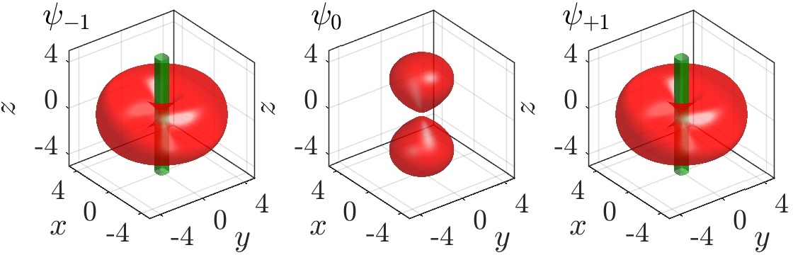
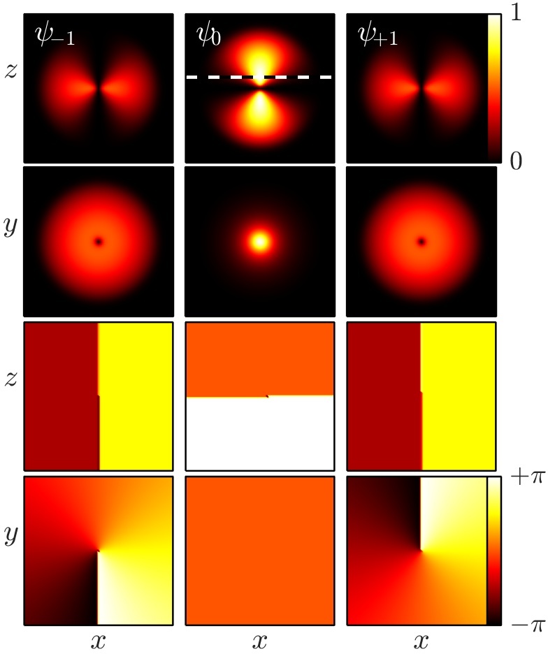
Figure 1: (Color online) Monopole solution for $\mu=20$ in an isotropic trap with $\Omega=1$. The top row of panels depicts isolevel cuts of constant density (red) and vorticity (green) for the components $\psi_{+1}$ (left), $\psi_{0}$ (middle) and $\psi_{-1}$ (right). Second and third (fourth and fifth) rows depict cuts of the respective densities (phases). All cuts pass through the origin except for the $(x,y)$ cuts for $\psi_{0}$ which are done through the plane of maximum density shown by the horizontal dashed line in the middle panel. For ease of presentation, the depicted densities have been normalized so that max($|\psi_{+1}|^{2},|\psi_{0}|^{2},|\psi_{-1}|^{2})=1$. The field of view for the cuts corresponds to $-7.5<x,y,z<7.5$ while the computational domain is $(x,y,z)\in[-L_{x},L_{x}]\times[-L_{y},L_{y}]\times[-L_{z},L_{z}]$ where $L_{x}=L_{y}=L_{z}=12$.

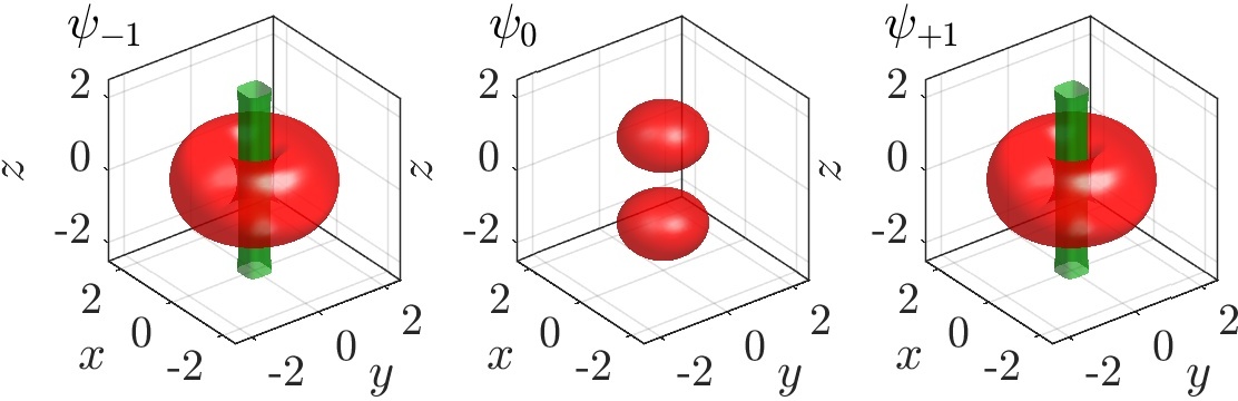
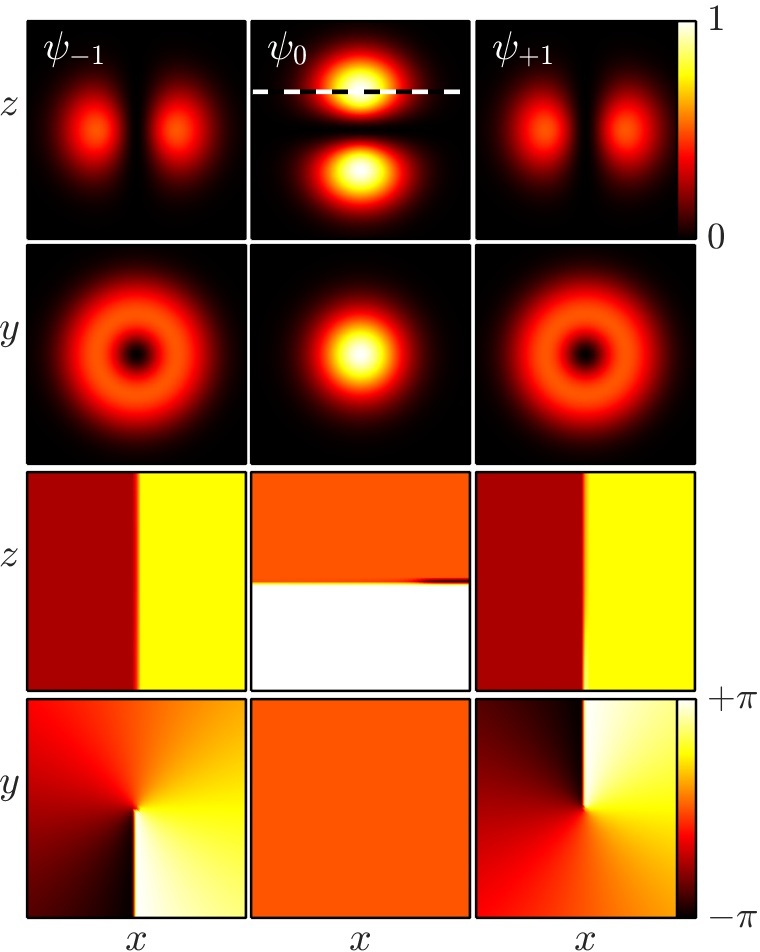
Figure 2: (Color online) Same as in Fig. 1 but for a monopole solution for $\mu=3.5$, i.e., close to the linear limit ($\mu=5/2$) which corresponds to a much lower atom number. The field of view for the cuts corresponds to $-3<x,y,z<3$.

III.1 Steady States

Steady states for the spinor BEC are obtained by considering stationary solutions of the form $\psi_{j}(\textbf{r},t)\rightarrow\psi_{j}(\textbf{r})e^{-i\mu_{j}t}$ in Eq. (7) for fixed (non-dimensional) chemical potentials $\mu_{j}$. From these equations and direct substitution, it can be immediately inferred that steady states are only possible if $\mu_{-1}+\mu_{+1}=2\mu_{0}$. Considering a symmetric split between the $\psi_{+1}$ and $\psi_{-1}$ components (i.e., $\mu_{+1}=\mu_{-1}$), implies that non-trivial configurations satisfy

$$\begin{split}(\mathcal{H}-\mu)\psi_{+1}+c_{2}(|\psi_{0}|^{2}+F_{z})\psi_{+1}+c_{2}\psi_{-1}^{\ast}\psi_{0}^{2}&=0,\\ (\mathcal{H}-\mu)\psi_{0}+c_{2}(|\psi_{+1}|^{2}+|\psi_{-1}|^{2})\psi_{0}+2c_{2}\psi_{0}^{\ast}\psi_{+1}\psi_{-1}&=0,\\ (\mathcal{H}-\mu)\psi_{-1}+c_{2}(|\psi_{0}|^{2}-F_{z})\psi_{-1}+c_{2}\psi_{+1}^{\ast}\psi_{0}^{2}&=0,\end{split}$$ (12)

where $\mu\equiv\mu_{-1}=\mu_{+1}=\mu_{0}$. Note that different values of $\mu$ will correspond to different total masses in the original system. Steady states are then computed using discretization methods and iterative solvers of the resulting coupled, nonlinear algebraic equations (see Appendix B.1 for more details). The initial seed is chosen to be a combination of a dark soliton (i.e., a quasi 2D planar structure) at $z=0$ in $\psi_{0}$ and vortex lines of charge $\pm 1$ in components $\psi_{\pm 1}$, and given by

$$\Psi=\begin{bmatrix}\psi_{+1}\\ \psi_{0}\\ \psi_{-1}\end{bmatrix}=\frac{\sqrt{n(\mathbf{r})}e^{i\phi}}{\sqrt{2}}\begin{bmatrix}-r_{x}+ir_{y}\\ \sqrt{2}r_{z}\\ r_{x}+ir_{y}\end{bmatrix},$$ (13)

with $\hat{\mathbf{r}}=(r_{x},r_{y},r_{z})=(x,y,z)/r$. Without loss of generality, we fix $\phi=0$, and we note that all components are modulated by their respective Thomas-Fermi (TF) density approximations, which, assuming large density (and chemical potential), uses

$$n(\mathbf{r})={\frac{\mu-V(\mathbf{r})}{c_{0}}},$$ (14)

when $\mu\geq V(\mathbf{r})$ and $0$ otherwise. In Figs. 1 and Fig. 2 we depict the converged steady-state solutions for $\mu=20$ and $\mu=3.5$, respectively. As the phase cuts and isolevel vorticity cuts depict, the $\psi_{+1}$ and $\psi_{-1}$ components contain a straight, vertical vortex line about the $z$-axis. Also, the mutual repulsion between the $\psi_{\pm 1}$ and $\psi_{0}$ components, along with the presence of the vortex line along the $z$-axis result in the $\psi_{\pm 1}$ densities being pushed in the plane $(x,y)$ radially out while the $\psi_{0}$ component splits into two domains along the $z$-axis separating regions of opposite phase (see respective phase cuts). The $\mu=3.5$ case corresponds to a configuration with small total mass (i.e., atom number) close to the linear limit ($\mu=5/2$; see below) of the governing equations, whereby ${\cal N}\rightarrow 0$. Comparing Figs. 1 and 2, it is evident that the width of the vortex line for $\mu=3.5$ is significantly larger than the corresponding one for $\mu=20$ as the corresponding healing length is inversely proportional to the square root of the chemical potential. Indeed, at the linear limit the vortex lines along the $z$-axis result from suitable linear combinations of the harmonic oscillator modes $|p,l,k\rangle$, corresponding to quantum numbers $p$, $l$, and $k$ along the three Cartesian directions. These vortex lines with topological charge $S=\pm 1$ arise from linear combinations $|1,0,0\rangle\pm i|0,1,0\rangle$ (for the components $\psi_{\pm 1}$) or similar, and the component $\psi_{0}$ features a dipolar state $|0,0,1\rangle$. All of these linear states are energetically degenerate at the linear limit with $p+l+k=1$ and hence correspond to energy $E=\Omega(p+l+k+3/2)=5/2$, as numerically identified above. This, in turn, suggests that the monopole state is a mode that directly emerges from the (first excited state within the) linear limit of the parabolically confined system, as showcased in Fig. 2 and exists all the way to the highly nonlinear (TF) limit thereof, as suggested in Fig. 1. The dependence of the corresponding atom number on the chemical potential in the path between these two limits can be visualized in Fig. 3.

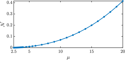
Figure 3: (Color online) Total (adimensionalized) atom number [cf. Eq. (5)] for the monopole solution as the (adimensionalized) chemical potential $\mu$ is varied. The monopole solution starts, in the linear limit, at $\mu=5/2$.

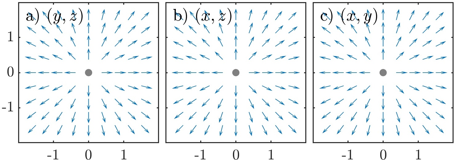
Figure 4: Projections along the $(y,z)$ (left), $(x,z)$ (middle) and $(x,y)$ (right) plane of the nematic vector for the monopole solution for $\mu=20$. The unequivocal hedgehog topology of the monopole (with the field pointing radially outwards) can be observed.

In order to showcase the monopole nature of the converged solutions, we compute the nematic vector field (also referred to as the director field). For a pure polar state (like the monopole solution), the nematic vector field can be computed by decomposing the spinor wavefunction through Eq. (11) where ${\mathbf{\hat{d}}}=(d_{x},d_{y},d_{z})^{T}$ is in general known as the nematic vector Tiurev et al. (2016). However, for general solutions with non-vanishing magnetization (as it will be the case of the AR solutions presented in the next section), the above description cannot be used. Instead, we rely on the method of nematic vector field calculation through the magnetic quadrupolar tensor Mueller (2004); Symes and Blakie (2017)

$${\mathcal{Q}}_{ab}=\frac{\zeta_{a}\zeta_{b}^{*}+\zeta_{b}\zeta_{a}^{*}}{2},$$ (15)

where the $\zeta_{j}$ ($j\in\{x,y,z\}$) are the normalized spinor components expressed in Cartesian coordinates Kawaguchi and Ueda (2012), namely $\psi_{j}=\sqrt{n}e^{i\phi}\zeta_{j}$, and

$$\left\{\begin{array}[]{rcl}\psi_{x}&=&\displaystyle\frac{\psi_{+1}-\psi_{-1}}{\sqrt{2}},\\[6.45831pt] \psi_{y}&=&\displaystyle i\frac{\psi_{+1}+\psi_{-1}}{\sqrt{2}},\\[6.45831pt] \psi_{z}&=&\displaystyle\psi_{0}.\end{array}\right.$$ (16)

Then, following the prescription of, e.g., Ref. Tiurev et al. (2016), one can extract the nematic vector by choosing, at each spatial location, the eigenvector of ${\mathcal{Q}}$ corresponding to the largest eigenvalue which corresponds to the local spin orientation of the order parameter. According to this method to compute the nematic vector, it should be noted that the factorization of the density and the global phase $\phi$ are irrelevant [the density is a common scalar factor of ${\mathcal{Q}}$ and the phase $\phi$ gets eliminated through the combinations such as $\psi_{a}\psi_{b}^{*}$ appearing in Eq. (15)]. Figure 4 depicts projections of the nematic vector along different planes of the relevant 3D structure for a typical monopole. As the figure shows, the nematic vector corresponds to a purely radial, outward field evidencing the monopole texture of the solution.

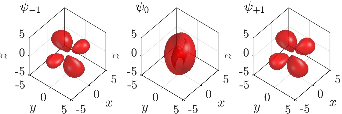
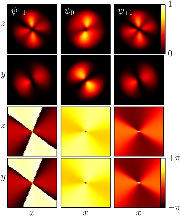
Figure 5: (Color online) Most unstable eigenfunction for the monopole solution for $\mu=20$ Top row of panels: isocontours for the density of most unstable eigenvector. Bottom four rows: cuts of the most unstable eigenvector. The first two rows correspond to density cuts and the last two to the corresponding phase. All cuts pass through the origin. Please refer to Appendices A and B.2 for details on the BdG formulation and the numerical methods involved.

III.2 Stability

Let us now characterize also the stability of the family of monopole solutions as a function of the chemical potential $\mu$. For that purpose we utilize the Bogoliubov-de Gennes (BdG), linear stability equations for small perturbations away from stationary fixed points; see Appendix A for details of the perturbation ansatz and the corresponding stability matrix. The outcome of this analysis yields the eigenvalues and eigenvectors of the linearization around the equilibrium state (here, the monopole) and showcases the potential spectral stability or instability of the examined nonlinear state.

It is interesting to highlight that the bifurcation of the monopole from the linear limit eigenvalue of $\mu=5/2$ already provides information about the number of potential instabilities of this excited state in the way of so-called negative energy modes Kevrekidis et al. (2015). Indeed, near the linear limit, extending the eigenvalue calculation of the single component case of Ref. Feder et al. (2000), we find that the BdG linearization operator of Appendix A becomes a diagonal one with $\hat{h}_{0}-\mu$ and $-(\hat{h}_{0}-\mu)$ along the diagonals. In this case, we can directly calculate the spectrum from the knowledge of the quantum harmonic oscillator one as: $\pm(p+l+k-1)$ for $\mu=5/2$ (with both sets of energies/eigenvalues measured in units of $\Omega$).

It is then straightforward to observe that the negative energy modes in each component will arise due to the $(p,l,k)=(0,0,0)$ state and hence, given the component multiplicity of components, there will be 3 such states. Similarly the 3 combinations $(1,0,0)$, $(0,1,0)$ and $(0,0,1)$ will result in vanishing eigenvalues for a total of 9 such, given the component multiplicity. Finally, e.g., the positive eigenvalues pertaining to $p+l+k=2$ will, through a similar count, be 6 per component and 18 in total. The important count among these different ones is that of the negative energy modes. Given the topological nature of such states, these modes will preserve the sign of their energy unless they collide with positive energy ones leading to an instability via the formation of a complex eigenvalue quartet. Indeed, this scenario does materialize near the linear limit for the monopole, where we find it to be unstable due to 3 complex eigenvalue quartets (data not shown). Nevertheless, the more general conclusion of relevance to all values of, e.g., the chemical potential is that such a monopole state carries the potential for up to 3 instabilities via such quartets at any value of $\mu$, due to the presence of these 3 negative energy modes.

Additionally, our computations show that the spectrum for the monopole features an instability with a positive real eigenvalue corresponding to an exponential instability. A typical most unstable eigenfunction for the monopole obtained on a $[-12,12]^{3}$ grid with $51^{3}$ points is shown in Fig. 5. Closer examination of this eigenvector reveals that it contains same signed lobes to either side of the original vortex lines of the steady-state solution. These lobes, when added to the steady state, will result in an effective displacement, along the $(x,y)$ plane, for the vortex lines in the $\psi_{\pm 1}$ components. This displacement is typical when adding an even eigenfunction to an odd solution (or vice-versa). It is important to note that, since the vortex lines in the $\psi_{-1}$ and $\psi_{+1}$ components have opposite charge, the displacement for each vortex line is in the opposite direction. Therefore, we expect that the initial destabilization of the monopole to be attributed to a symmetry breaking scenario where the vortex lines in the $\psi_{\pm 1}$ components separate and drift away from the trap’s center (which will be corroborated through direct numerical integration; see below).

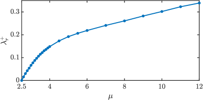
Figure 6: (Color online) Most unstable (real) eigenvalue for the monopole solution as a function of the chemical potential $\mu$, depicting the growth rate associated with the corresponding eigendirection.

Figure 6 depicts the instability growth rate, through the positive real part, denoted as $\lambda_{r}^{+}$ hereafter of the most unstable eigenvalue, of the monopole solution as a function of the chemical potential (see Appendix B.2 for details on the numerical computations). As the figure indicates, as one gets closer to the linear limit where the monopole solution is born ($\mu=5/2$), the real part of the relevant eigenvalue tends to zero. Besides the unstable real eigenvalue (and its negative sibling owing to the Hamiltonian nature of the problem) with triple multiplicity, the spectrum is composed of a set of purely imaginary eigenvalues and a zero eigenvalue with multiplicity eight. The zero eigenvalues are associated with the symmetries (or invariances) of the corresponding steady-state solution and equations. In particular, we note in that connection that the monopole can be rotated around any direction, in addition to its possessing an overall phase invariance, associated with the total atom number conservation law. On the other hand, the purely imaginary eigenvalues consist of (i) the spectrum related to the ground state of the system and (ii) negative energy modes associated with the excited state nature of the monopole configuration of interest here.

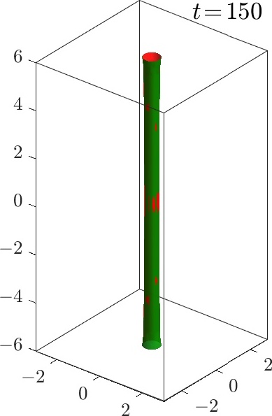
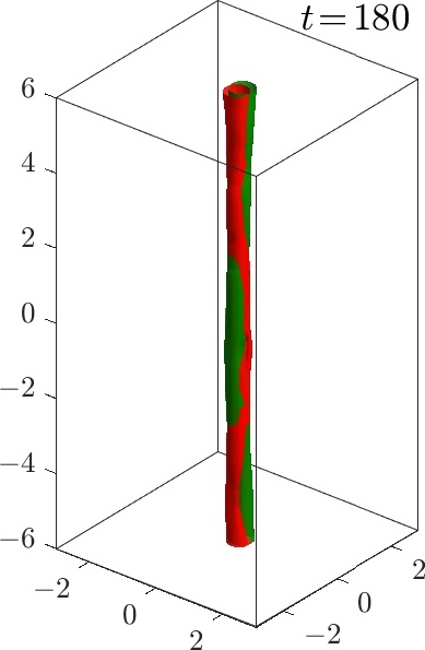
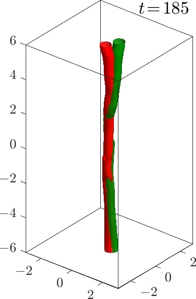
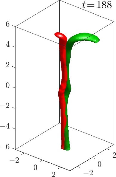
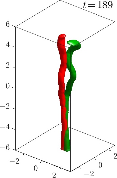
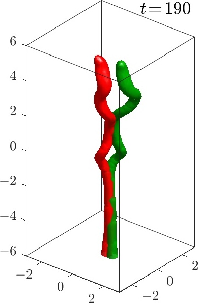
Figure 7: (Color online) Destabilization dynamics for the monopole solution with $\mu=20$ at the indicated times. Shown are overlaid isocontours for the vorticity corresponding to the $\psi_{+1}$ (red) and $\psi_{-1}$ (green) components. The system was initialized with the numerically exact steady state monopole solution with a spatial random perturbation of size $10^{-8}$ (relative to the steady state size). For the corresponding movie please follow this link.

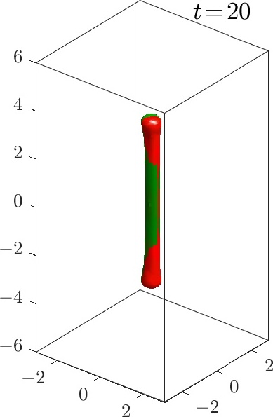
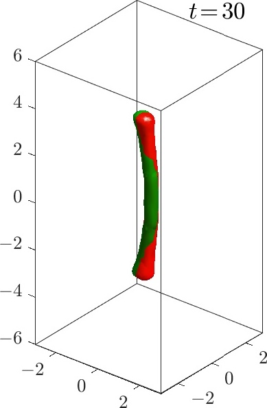
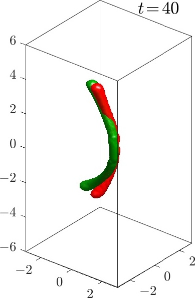
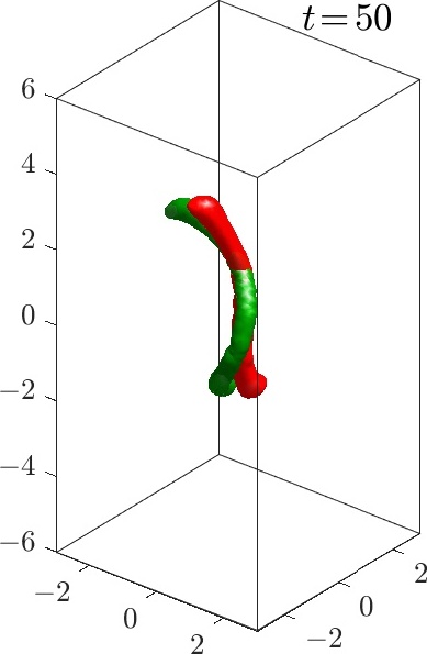
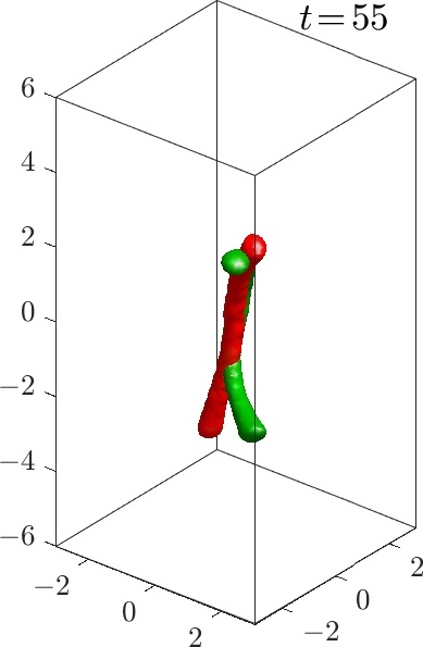
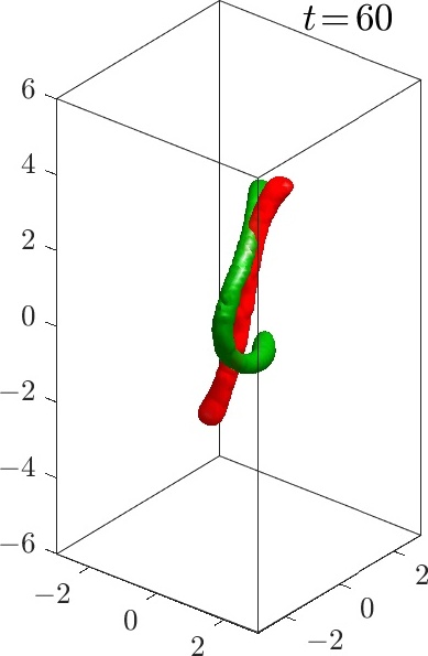
Figure 8: (Color online) Same as in Fig. 7 but for $\mu=4$. For the corresponding movie please follow this link.

III.3 Dynamics

Let us now follow the dynamical destabilization of the monopole solution by directly integrating the equations of motion initialized by slightly (randomly) perturbed stationary configurations. The cases for $\mu=20$ and $\mu=4$ are depicted in Figs. 7 and 8, respectively. As we are mainly interested in the fate of the vortex lines present in the $\psi_{\pm 1}$ components, we only show overlays of their corresponding isocontours of vorticity. In line with the eigenvector stability results above, we see that the destabilization of the monopole evolves through a symmetry breaking between the vortex lines in the $\psi_{\pm 1}$ components. We typically observe that the vortex lines slightly split from one another and start slowly drifting away from the $z$-axis. The drift is tantamount (albeit not exactly equivalent, since here the vortex lines pertain to different components) to the behavior of adjacent vortex lines in one-component BECs. There, vortex lines of same charge tend to rotate around each other while vortex lines of opposite charge (as is the case for our system) tend to travel parallel to each other. In general we observed that, eventually, the vortex lines separate further and more complex dynamics ensues, particularly for higher values of $\mu$ where the vortex lines are thin and prone to undulations (Kelvin waves) Kevrekidis et al. (2015). However, we would like to focus on a particularly prevalent feature that is common to most monopole configuration destabilization dynamics for high enough chemical potential.

As an example, close inspection of the destabilization dynamics for $\mu=20$ (see Fig. 7) reveals that the vortex lines tend to mainly split from each other at the edges of the cloud and, more importantly, around the center of the trap. The split at the cloud’s periphery is eventually responsible for the “peeling” off of the two vortex lines and the eventual complex vortex line dynamics. However, before entering this fully developed filamentary dynamics, the split between the vortex lines at the center of the trap creates a small bulge in the shape of a ring composed of two halves, one from each of the $\psi_{\pm 1}$ components. Namely, as clearly seen in the $t=188$ panel of Fig. 7, the vortex lines develop a ring around the trap’s center. This configuration is reminiscent of an AR, first studied in detail in the present BEC context in Ref. Ruostekoski and Anglin (2003), which we study in more detail in the next section of this work.

It is interesting that as part of the destabilization of the monopole, due to the central splitting of the vortex lines across the $\psi_{\pm 1}$ components, the dynamics tend to “hover” momentarily through a solution akin to an AR. While transiently we observe such a ring configuration in a segment of the condensate, over long time scales the dynamics of the monopole involves multiple recurrences and an eventual split of the vortex lines and a disappearance of the associated vorticity towards the background (TF) cloud. It is also relevant to comment that the dynamics of Fig. 8 similarly illustrate the peeling off of the vortex lines at the edges, yet are far less suggestive towards the creation of a potential ring near the center of the trap. We attribute this to the important feature (as we will see below) stemming from our analysis of ARs that such structures do not exist at such low values of the chemical potential. Hence, they are no longer natural candidates for such transient dynamical observations in this case of lower chemical potential.

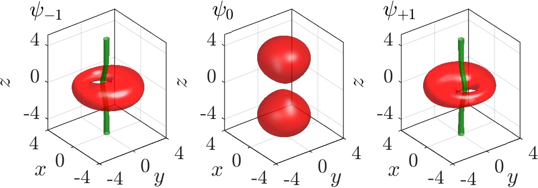
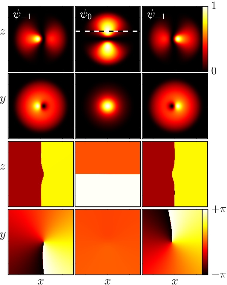
Figure 9: (Color online) First Alice ring (AR) solution for $\mu=20$. Same layout as in Fig. 1, with isolevels of density (red) and vorticity (green) in the top row and different cuts, clearly showcasing the “symmetry breaking” nature of the AR structure are shown in the 2nd-5th rows along the different planes and for the different components.

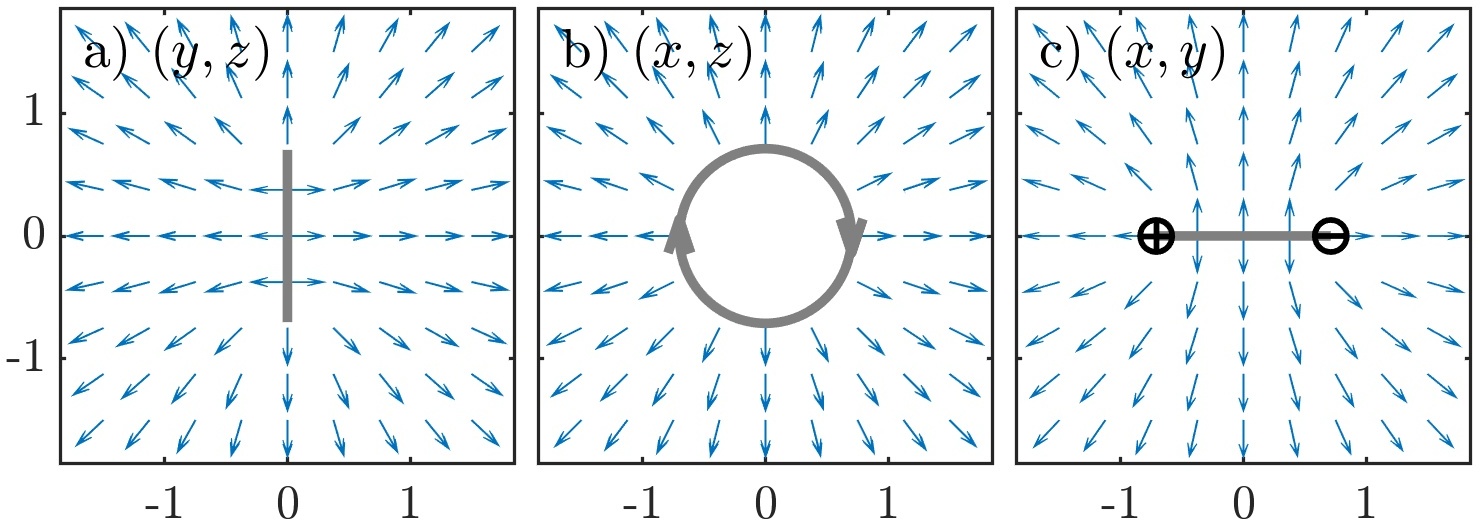
Figure 10: Nematic vector for the first AR solution for $\mu=20$. In contrast with the monopole depicted in Fig. 4, the AR has a disk (inside the ring itself) where the nematic vector field abruptly reverses direction. Nonetheless, the AR’s far field does match the one for the monopole. The grey curves depict the location of the AR and the ‘$+$’ and ‘$-$’ symbols in panel c) highlight the location of the vortices in the $\psi_{+}$ and $\psi_{-}$ components, respectively.

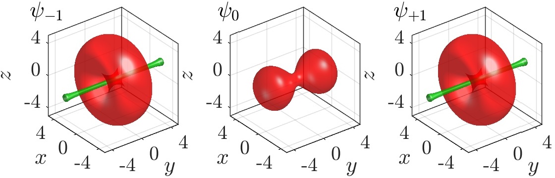
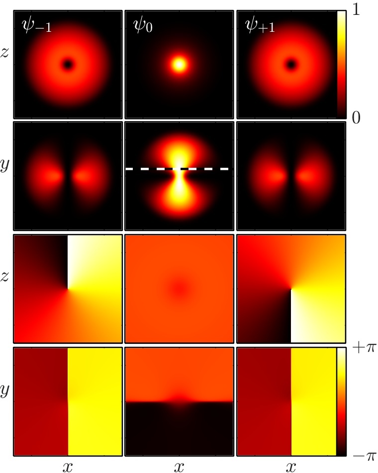
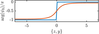
Figure 11: (Color online) First Alice ring solution for $\mu=20$ with quantization axis perpendicular to the plane of the ring (i.e., parallel to the $y$-axis). In this basis it is apparent that the superfluid density is nonzero and the phase changes smoothly by approximately $\pi$ in the region along the $y$-axis. This solution is obtained by applying a rotation in spin space with Euler angles $\alpha=\gamma=0$ and $\beta=\pi/2$ (cf. Eq. (551) in Ref. Kawaguchi and Ueda (2012)). Top panel: same layout as in Fig. 9. Bottom panel: phase corresponding to $\psi_{0}(0,0,z)$ (blue) and $\psi_{0}(0,y,0)$ (orange) for the first AR in, respectively, spinor coordinates (cf. Fig. 9) and with the quantization axis parallel to the $y$-axis (see top panels).

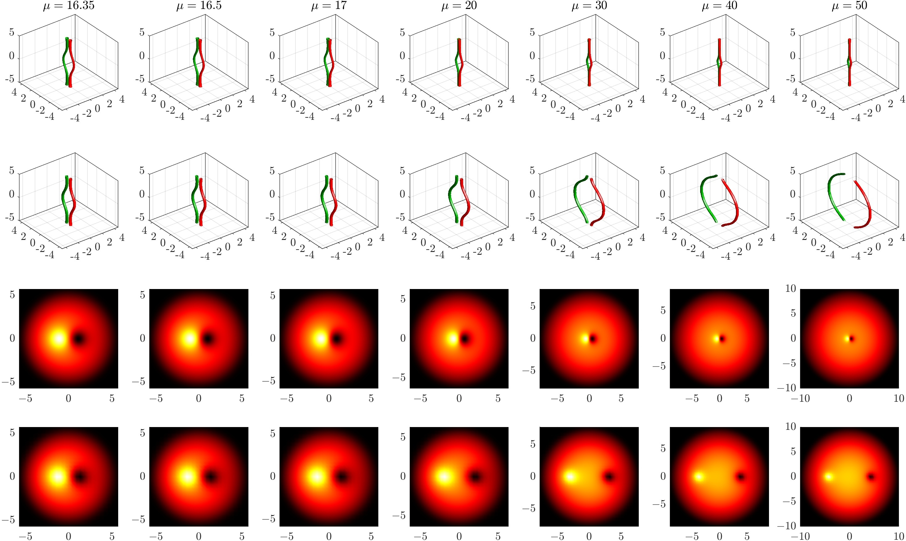
Figure 12: (Color online) AR steady states for different values of $\mu$ as indicated in the panels. The first and third row of panels correspond to the first AR branch (smaller rings) while the second and fourth rows correspond to the second AR branch (larger rings). The top two rows of panels depict the isolevel cuts of constant vorticity for the $\psi_{+1}$ (green) and $\psi_{-1}$ (red) components. The bottom two rows of panels depict the corresponding $z=0$ cut of the density for the $\psi_{-1}$ component. Note that the plotting window for the density cuts is rescaled by the TF radius $R_{\rm TF}$ as $[-1.5R_{\rm TF},1.5R_{\rm TF}]{\mkern-1.0mu\times\mkern-1.0mu}[-1.5R_{\rm TF},1.5R_{\rm TF}]$ to keep the apparent size of the cloud constant.

IV Alice Rings

An AR corresponds to a half-quantum vortex ring which resembles a monopole solution Kawaguchi and Ueda (2012); Ruostekoski and Anglin (2003) far from the origin of the structure. In this structure, a $\pi$ change in the global phase $\phi$ is accompanied by a $\pi$-disclination of the quantization vector $\hat{\mathbf{d}}$. Indeed, the singular point defect of the ’t Hooft-Polyakov monopole setting deforms itself into a ring structure where half the ring consists of the (deformed) vortex line of the $\psi_{1}$ component, while the other half of the (symmetrically deformed in the opposite direction) vortex line of the $\psi_{-1}$ component. Thus, it is not surprising to expect that, as already hinted above, that the dynamical instability of the monopole is intimately connected with the dynamical emergence of the AR.

IV.1 Steady States

Inspired by the appearance of the vortex line bulge close to the center in the dynamical destabilization of the monopole solution, we initialize our steady-state optimizer with a snapshot of the monopole destabilization when the bulge is visible but before the vortex lines bend and twist themselves, substantially detaching from each other. By doing so, we are able to identify a stationary AR solution and follow it for different values of the chemical potential. For instance, Fig. 9 depicts the AR solution for $\mu=20$ where we clearly see the bulge of the vortex lines in opposite directions for the $\psi_{+1}$ and $\psi_{-1}$ components. We call this solution the first AR since, as we will reveal below, there is another branch of AR solutions (the second AR). Figure 10 depicts the nematic vector for a typical AR. The nematic vector field shows that, as the vortex lines in the $\psi_{\pm 1}$ open up and create a ring, the far field still corresponds to the hedgehog (radially outward) structure of a monopole. The principal new feature in this representation is the presence of a $\pi$-discontinuity of the nematic vector across the plane of the ring. Although the nematic (director) vector is discontinuous on the AR disk, the $\mathbb{Z}_{2}$ nematic symmetry $(\hat{\mathbf{d}},\phi)\rightarrow(-\hat{\mathbf{d}},\phi+\pi)$ permits $\Psi$ to remain continuous provided the discontinuity in the direction of $\hat{\mathbf{d}}$ is accompanied by a discontinuity of $\pi$ in the phase $\phi$. Given that the director orientation and the phase are thus not uniquely prescribed, we return to the full solution of $\Psi$ for an in-depth account of the AR.

The crucial topology of the AR manifests itself in the nonzero superfluid density along the $y$-axis, and perpendicular to the plane of the ring, which disrupts the solitonic structure associated with its parent monopole. This feature is most easily discerned in the $m=0$ spinor component density in a basis quantized along the $y$-axis (see Fig. 11). Moreover, the condensate phase changes continuously by approximately $\pi$ along the axis (see orange curve in bottom panel), as is expected for a half-quantum vortex ring —contrast this phase variation with that for the AR represented in the original spinor basis of Fig. 9 which displays a discontinuous jump over its axis (see blue curve in the bottom panel of Fig. 11). It is interesting to note how the two different choices of quantization axis reveal complementary information: when quantized along $y$ (Fig. 11) the nonzero density in the $m=0$ spinor component defines the radius of the ring in the $(x,z)$ plane and the $\pi$ phase winding, whereas when quantized along $z$ (Fig. 9) the $m=\pm 1$ spinor components in the $(x,y)$ plane feature a structure reminiscent of a half-quantum vortex dipole. Also, interestingly, in the former case, the vortex lines in the $m=\pm 1$ components end up aligned, while in the latter feature a misaligned portion where each component traces half of the AR. These complementarities are reminiscent of the vortex-vortex states and their SU(2) rotations considered earlier in Ref. Charalampidis et al. (2016). All of the obtained AR solutions for the different parameters considered (variations of the chemical potential and trapping strengths), including the second AR branch (see below), display this general structure.

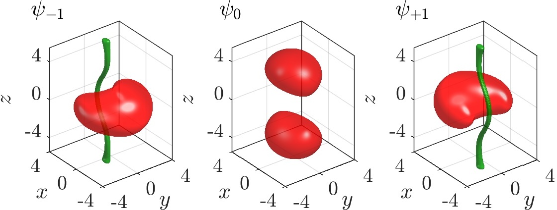
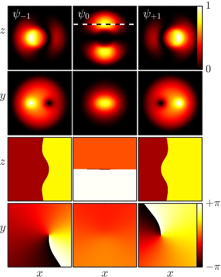
Figure 13: (Color online) Second AR solution for $\mu=20$. Same layout as in Fig. 9.

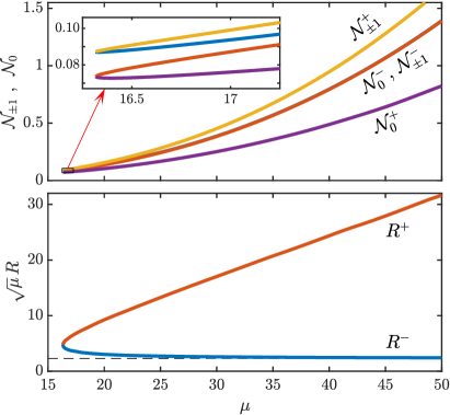
Figure 14: (Color online) Top: (adimensionalized) Atom numbers (6) for the AR solution as the (adimensionalized) chemical potential $\mu$ is varied. The AR solution seems to terminate, as $\mu$ decreases, at $\mu\approx 16.35$. Bottom: AR’s radius vs. chemical potential $\mu$. The radius has been normalized by $1/\sqrt{\mu}$. The horizontal dashed line corresponds to $R=2.3/\sqrt{\mu}$. The $-$ and $+$ superscripts correspond, respectively, to the first (small) and second (large) AR solutions.

Let us now discuss our parametric variation of the relevant AR waveforms. Once we obtained a genuine AR solution for a particular value of the chemical potential $\mu$, we used numerical continuation to follow this (first) solution branch for different values of $\mu$ as depicted in the first and third rows in Fig. 12. Interestingly, the first AR solution branch seems to not exist for values of $\mu<16.35$ and, thus, cannot be constructed all the way down to the linear (small mass) limit. Therefore, we sought a companion branch of solutions using arclength continuation Doedel and Tuckerman (2000) around $\mu<16.35$, upon identifying that this branch of solutions spontaneously emerges (out of the “blue sky”) for values of $\mu\geq 16.35$.

The arclength continuation reveals that indeed the first AR solution branch is connected to a second AR branch through a saddle-center bifurcation. The two AR solution branches collide at the relevant turning point. After going over the fold using arclength continuation, we are able to follow the second AR branch for larger values of $\mu$. For instance, Fig. 13 depicts a sample configuration of this second AR solution for $\mu=20$. More elements of this second AR branch are depicted in the second and fourth rows of Fig. 12. It is interesting that the first branch corresponds to smaller rings when compared to the second branch and that, as $\mu$ increases, the smaller rings of the first branch get smaller while the larger rings of the second branch get larger. I.e., it is interesting to observe that in a sense the AR emerges at a “critical radius” for $\mu\approx 16.35$ and thereafter the first branch approaches progressively (for increasing chemical potential) the monopole solution with the ring “closing in” by shrinking its radius, while the second branch progressively tends to grow with the curved segments of the vortex lines expanding toward the periphery of the cloud. However, it is relevant to keep in mind that the TF cloud edge also expands as $\mu$ increases (see also the comment below).

We have confirmed that the same qualitative behavior for the nematic vector, as depicted for the first AR in Fig. 10, is also present for the AR members of the second family (results not shown here). In order to better depict the two AR branches within the same “bifurcation diagram”, the top panel of Fig. 14 depicts the (dimensionless) atom number of the AR branches as a function of $\mu$. The bottom panel of Fig. 14 depicts the radius of the (smaller) first ($R^{-}$) and (larger) second ($R^{+}$) ARs normalized by $1/\sqrt{\mu}$. The ring radii are extracted by determining the position of the positively and negatively charged vortices present in the 2D cuts of the $\psi_{\pm}$ components on the $z=0$ plane. Apparently, the rescaled radius $R^{+}$ for the second AR family increases linearly with $1/\sqrt{\mu}$ as $\mu$ increases. This indicates that $R^{+}\propto\sqrt{\mu}$ which means that indeed $R^{+}$ it increases linearly with the size (Thomas-Fermi radius $R_{\rm TF}\propto\sqrt{\mu}$) of the condensate cloud —this is also apparent in the larger $\mu$ yet $z=0$ cuts in the fourth column of panels in Fig. 12 where the relative position of the vortices with respect to condensate cloud edge seems to be constant. In contrast to the enlarging behavior of the second AR family, the first ring family tends to shrink as $\mu$ increases. In fact, the first AR radius seems to tend to a constant fraction of $1/\sqrt{\mu}$ as $\mu\rightarrow+\infty$.

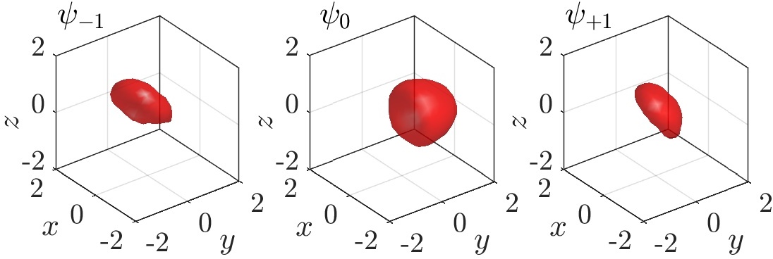
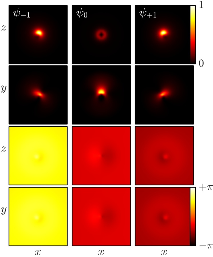
Figure 15: (Color online) Most unstable eigenfunction for the first AR solution for $\mu=20$; same layout as in Fig. 5. The most unstable eigenvector does not carry a sizeable amount of vorticity and thus isocontours of vorticity have been omitted. Please refer to Appendices A and B.2 for details on the BdG formulation and the numerical methods involved.

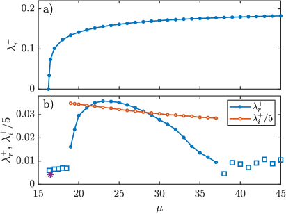
Figure 16: (Color online) Dominant (most unstable) eigenvalues for the first (top panel) and second (bottom panel) AR families as a function of $\mu$. (Blue) Dots and squares correspond to the real part of the eigenvalue, while the empty (orange) dots correspond to the imaginary part of the eigenvalue (rescaled by a factor of 5). The first AR family always exhibits a purely real eigenvalue indicating a dominant exponential instability. For the second AR, both, the small (blue) dots and (blue) squares, correspond to numerics performed with a grid of 121$\times$121$\times$121 mesh points. The (blue) dots correspond to an oscillatory instability while the (blue) squares correspond to an apparently spurious set of exponential instabilities resulting from the discretization effects in the numerics. The (purple) asterisk corresponds to more refined numerics using a grid of 153$\times$153$\times$153 mesh points.

IV.2 Stability

Let us now study the stability properties of the AR solution. Figure 15 depicts a typical most unstable eigenvector for the first AR solution for $\mu=20$. As for the monopole, this AR solution is unstable with a positive real eigenvalue corresponding to an exponential instability. As far as the eigenvector is concerned, a similar conclusion as with the corresponding one for the monopole ensues. Namely, the eigenvector bears a different symmetry structure than the vortex line solutions in the $\psi_{-1}$ and $\psi_{+1}$ components, and, thus, when added to them induces a (larger) separation between the vortex lines. Figure 16 depicts the instability rate for both the first (top panel) and the second (bottom panel) AR families as a function of $\mu$. As mentioned above, both AR families emerge around $\mu=16.35$ in a saddle-center bifurcation as suggested by the figure. The first AR is clearly unstable bearing an exponential instability over the range of chemical potentials studied. On the other hand, in the case of the second AR shown in the bottom panel, extrapolation of the eigenvalues for even finer meshes suggests that the eigenvalues depicted by the (blue) squares are spurious. In fact, as detailed in the Appendix B.2 (see Fig. 21), as the number of mesh points ($N{\mkern-1.0mu\times\mkern-1.0mu}N{\mkern-1.0mu\times\mkern-1.0mu}N$) increases, these (spurious) eigenvalues tend to zero according to the power law $\propto 1/N$. This strongly suggests that the second AR is indeed spectrally stable in the region $16.35\leq\mu\lesssim 19$ and $\mu\gtrsim 38$; namely before and after it incurs a bubble of oscillatory instabilities (for which we can also identify and show within the panel the relevant imaginary part). Furthermore, not only does the extrapolation of the eigenvalues for finer meshes suggest that the second AR is stable, but this is also in line with the generic bifurcation-theory-based expectation for a saddle-center bifurcation where the second AR is the stable sibling of the first (unstable) AR at the bifurcation point.

As the chemical potential is further increased, while the first AR branch retains its exponential instability mode, the second branch AR solutions transition, around $\mu\approx 19$, to an instability with a dominant complex eigenvalue quartet indicating an oscillatory instability. Finally, as $\mu$ is increased further ($\mu\gtrsim 38$), the oscillatory instability recedes and the second AR recovers its stability. This oscillatory instability bubble (window) for $19\lesssim\mu\lesssim 38$ emerges when two pairs of opposite Krein signature Kevrekidis et al. (2015) eigenvalues collide, on the imaginary axis, and eject as a quartet with non-zero real parts, in line with our earlier discussion of such features in the vicinity of the linear limit for the case of the monopole.

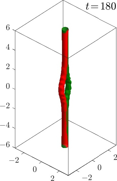
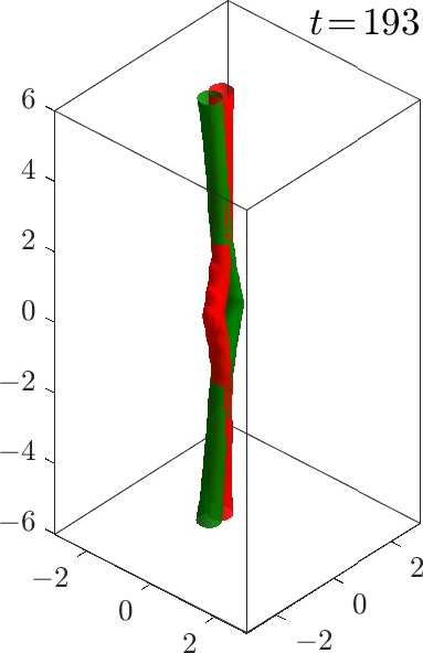
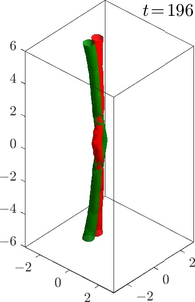
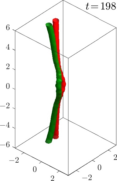
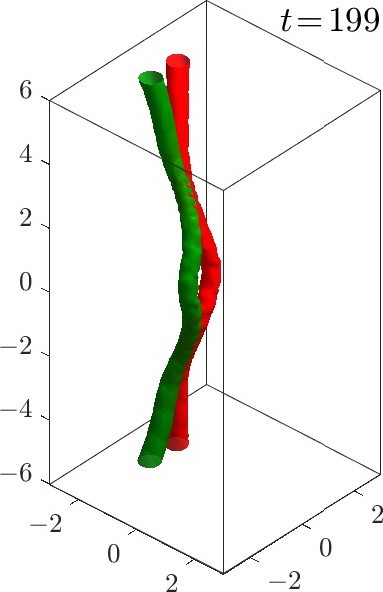
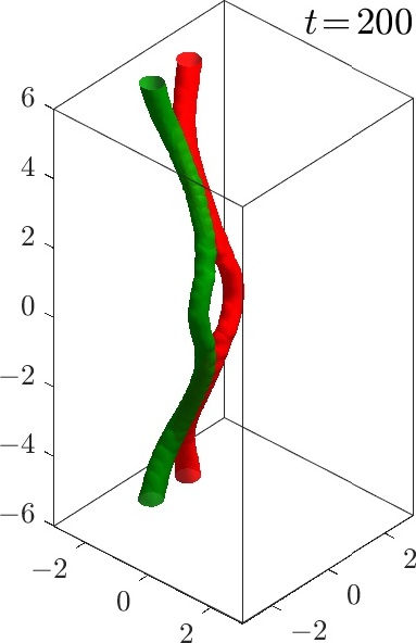
Figure 17: (Color online) Destabilization dynamics for the first AR for $\mu=25$. Same layout and perturbation as in Fig. 7. For the corresponding movie please follow this link.

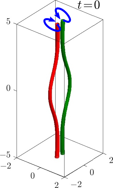
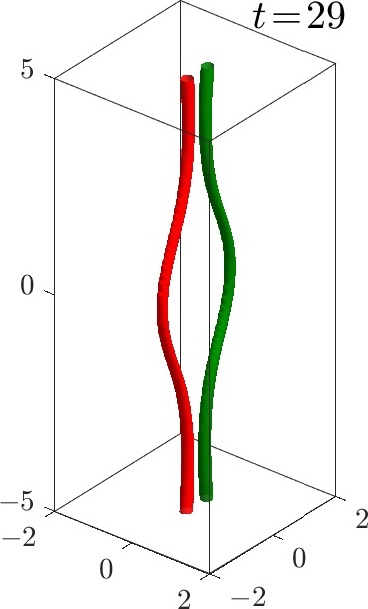
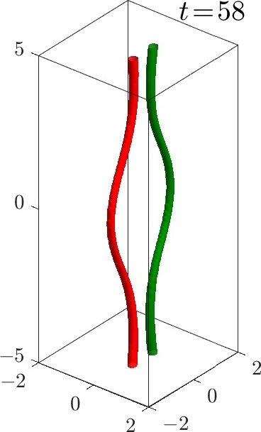
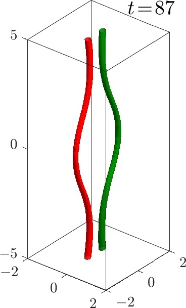
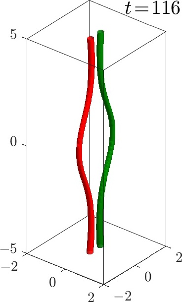
Figure 18: (Color online) Destabilization dynamics for the first AR for $\mu=16.5$ giving rise to a homoclinic orbit. The vortex filaments move in a cycle depicted by the blue arrows in the first panel. Same layout and perturbation as in Fig. 7. For the corresponding movie please follow this link.

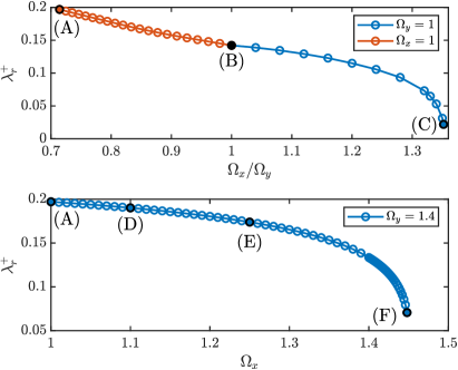
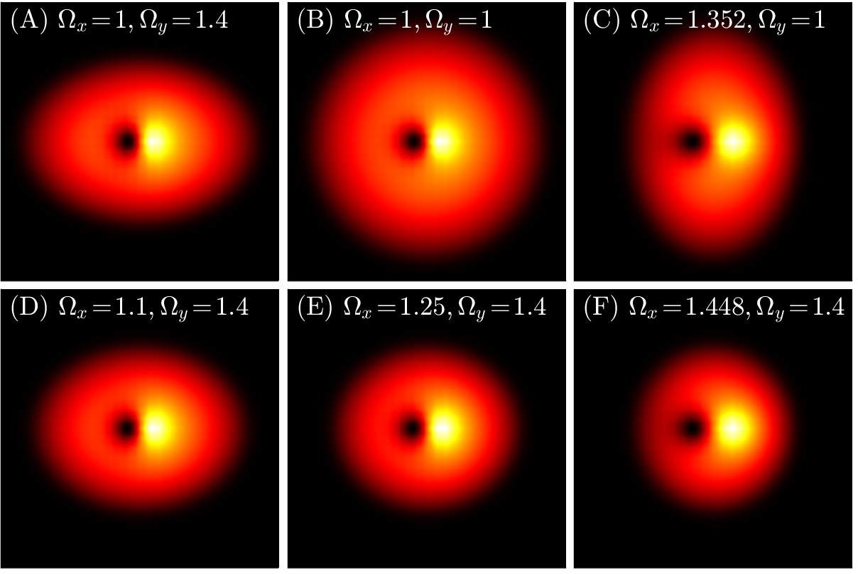
Figure 19: (Color online) Most unstable eigenvalue (purely real) for the first AR solution for $\mu=20$ and several trap strength combinations. Top: To the left of the isotropic case $\Omega_{x}=\Omega_{y}=1$ (see black dot) the trap is oblate with $\Omega_{y}>1$ and $\Omega_{x}=1$; while to the right of the isotropic case the trap is prolate with $\Omega_{x}>1$ and $\Omega_{y}=1$. The solution cannot be continued for larger $\Omega_{x}$ values past the point (C). Middle: A tighter trap with $\Omega_{x}=1$ and $\Omega_{y}>1$. The solution cannot be continued for larger $\Omega_{x}$ values past the point (F). The bottom set of panels depicts the density of the $\psi_{+1}$ component at $z=0$ corresponding to the different points labelled in the top two panels. The field of view corresponds to $(x,y)\in[-7,7]\times[-7,7]$.

IV.3 Dynamics

Figure 17 depicts the destabilization for the first AR for $\mu=25$. As mentioned above, the destabilization from the most unstable eigenvector tends to displace the vortex lines in the $\psi_{-1}$ and $\psi_{+1}$ components. As Fig. 17 shows, this displacement tends to shrink the diameter of the AR, and at the same time tends to separate the (previously coincident) ends of the vortex lines across components. As a result of the above rearrangements, the AR acquires an effective non-zero velocity and starts to advance towards $y>0$ while the vortex lines, being reversed with respect to each other when compared to the half ring on each side of the AR (see the figure), tend to move in the opposite ($y<0$) direction. As a result the vortex lines develop a strong undulation that eventually has the two vortex lines perform complex interactions (results not shown here). A particularly pronounced feature of these interactions is the separation/deviation from the aligned state of the vortex filaments (of the $\psi_{\pm 1}$ components) in the far field.

Finally, in Fig. 18 we depict an interesting case for the destabilization dynamics of a first AR for $\mu=16.5$ where, after doing a circular excursion away from the origin, the vortex filaments come back (very close) to their original location. This type of dynamics suggests the possibility for the existence of homoclinic as well as periodic orbits with non-trivial vortex filament dynamics. Indeed, this is at the heart of the characterization of this bifurcation as a saddle-center one: the dynamics apparently departs along the unstable manifold of the saddle and performs an oscillation around the stable center (i.e., the second AR), before nearly returning along the stable manifold of the saddle. Of course, the full PDE dynamics is more complex than this simple normal-form-based picture, yet for substantially long times, the PDE closely reflects this effectively one degree-of-freedom perspective. Further time integration of the evolution presented in Fig. 18 tends to destabilize the filaments in a similar manner as the interactions depicted in Fig. 17.

IV.4 Towards Stabilization of the First Alice Ring

Finally, we briefly summarize our attempts to stabilize the first AR solution which was found to be unstable for all the parameter values that we used in the case of an isotropic trap. Note that we did not try to study the effects of stabilization for the second AR as this solution already has a window of stability close to its bifurcation inception. The idea to tame the instability of the first AR relies on using the flexibility given by manipulating the trapping strengths along the different spatial directions to create an anisotropic trapping potential that might suppress the destabilization along a particular direction. For instance, Fig. 19 depicts our attempts to stabilize the first AR by keeping $\Omega_{z}=1$ and varying $\Omega_{x}$ and $\Omega_{y}$. The top panel shows the most unstable (real) eigenvalue along two different solution branches. The left (orange) branch corresponds to an oblate trap with $\Omega_{x}=1$ and $\Omega_{y}>1$, while the right (blue) branch corresponds to a prolate trap with $\Omega_{y}=1$ and $\Omega_{x}>1$; see the corresponding $\psi_{+1}$ cuts labelled (A) oblate, (B) isotropic, and (C) prolate in the lower panels of the figure. These results tend to suggest that a prolate trap with $\Omega_{y}=1$ and $\Omega_{x}>1$ is able to attenuate the instability of the first AR. Unfortunately, this AR solution cannot be continued past $\Omega_{x}\approx 1.352$ [see point (C)]. Nonetheless, a noticeable reduction of the instability growth rate can be achieved in this prolate limit. Finally, encouraged by these stabilization results, we also tried a tighter trap by letting $\Omega_{y}=1.4$ and increasing $\Omega_{x}$. The stabilization results are presented in the second panel of Fig. 19. In this case we again see a tendency towards stabilization as $\Omega_{x}$ is increased. However, as before, the solution ceases to exist for larger $\Omega_{x}$ values [$\Omega_{x}\approx 1.448$; see point (F)] before complete stabilization is achieved. In short, we have been able to use the manipulation of the trap strengths towards the reduction of the instability growth rate of the first AR solution. Nonetheless, we have not been able to fully suppress the relevant instability of this AR through such trap variations. It is worthwhile to note that the work of Ref. Ruostekoski and Anglin (2003) claims the complete stabilization of their AR via a pair of blue-detuned focused Gaussian laser beams. However, in the study herein, our focus was to study only the role of the most ubiquitous magnetic trap setting rather than towards the inclusion of additional forms of confinement.

V Conclusions and Future Work

In the present work, we explored the existence, stability, and dynamics of monopole and Alice ring (AR) solutions in a polar (anti-ferromagnetic) $F=1$ spinor condensate. Our study was primarily numerical in nature but it was critically assisted in the obtained understanding by theoretical limits such as the linear and the large density (Thomas-Fermi) ones, and notions such as those of the director vector and the magnetic quadrupolar tensor, the BdG spectral analysis and the evolution of the vorticity field among others. The monopole solution was found to emanate from the linear (low density) limit as the combination of opposite sign, overlapping, vortex lines in the $\psi_{+}$ and $\psi_{-}$ components and a domain wall (bearing a planar phase jump) in the $\psi_{0}$ component. The monopole solution was found to be unstable for all chemical potentials that we tested through a pair of real eigenvalues associated with an exponential instability. Interestingly, for large enough chemical potentials, the instability of the monopole typically forms, in the first time interval of its destabilization, a transient profile where the two vortex lines bulge locally near the center creating a ring completed by two halves corresponding to each vortex line across the $\psi_{\pm 1}$ components.

Motivated by such transient waveforms from the monopole destabilization and leveraging such a singular ring profile into a fixed point iteration procedure revealed the existence of a stationary ring structure. By analyzing the corresponding nematic vector we corroborated the fact that this stationary state corresponds to an AR whose topological texture in the far field matches the monopole (radial outward field), yet it contains a $\pi$-disclination of the nematic phase vector across the ring. Continuation analysis over the chemical potential reveals that the AR comes in two sizes: a smaller and a larger AR. These two AR families are found to collide in (i.e., bifurcate through) a saddle-center scenario at a critical value of the chemical potential, and the two solutions co-exist past this turning point as the chemical potential is increased. The smaller AR was found to always be unstable with a purely real (exponential) instability. In contrast, although finite-size numerics display a small instability for the larger ring, extrapolation of the associated eigenvalues for finer and finer meshes reveal a power-law decay for this instability. This is strongly suggestive that these small instabilities are spurious and induced by the mesh discretization and that the larger ring is indeed spectrally stable close to its bifurcation with the other ring. The larger ring is stable from its inception until it destabilizes for a chemical potential window (or bubble) with an oscillatory instability. As the chemical potential is increased further, this oscillatory instability disappears and the larger AR seems to regain its stability.

In an attempt to stabilize the smaller AR we probed its stability when the trapping deviated from its isotropic (spherical) starting point. Our results suggest that a prolate trap is able to attenuate the instability for the smaller AR but, unfortunately, is not enough to render it stable in the parameter regimes that we explored. Nonetheless, this noticeable attenuation of the instability might facilitate the observability of the smaller AR in addition to the larger AR which is stable for suitable values of the chemical potential.

It is, of course, relevant to note here that experiments such as those of Ref. Ollikainen et al. (2017) for monopoles and also, e.g., those of Refs. Hall et al. (2016); Lee et al. (2018) for other complex topological patterns such as quantum knots strongly suggest that the configurations presented herein are possible to realize in the current experimental state-of-the-art. Moreover, one can think of numerous directions of potential extensions of the present work to more complex settings. On the one hand, including additional optical potentials and exploring modifications to the branches of solutions presented herein (and, importantly, their stability) is an important future step, in line also with the original suggestion of Ref. Ruostekoski and Anglin (2003). On the other hand, and perhaps even more challengingly, one can consider extensions of the present setting into the 5-component setting of $F=2$ Kawaguchi and Ueda (2012). While it is natural to consider extensions of the monopole state in the latter setting, notions such as the one of the AR are far more elusive for $F=2$ and to the best of our knowledge have never been systematically examined in either numerical or physical experiments. Such studies are currently in progress and will be reported in future publications.

Appendix A Linearized GP equations

The adimensionalized GP equations [cf. Eqs. (7)] can be cast in the matrix form

$$i\frac{\partial\Psi}{\partial t}=\left(\mathcal{H}+c_{2}A\right)\Psi,$$ (17)

where

$$\mathcal{H}=-\frac{1}{2}\nabla^{2}+V(\textbf{r})+c_{0}n,$$

and

$$A=\begin{bmatrix}n_{+1}+n_{0}-n_{-1}&0&0\\ 0&n_{+1}+n_{-1}&0\\ 0&0&n_{-1}+n_{0}-n_{+1}\end{bmatrix},$$

where we recall that $n_{i}=|\psi_{i}|^{2}=\psi_{i}^{\ast}\psi_{i}$. Then, by following the corresponding evolution about the steady state $\Psi_{0}=(\psi_{+1},\psi_{0},\psi_{-1})$, the solution $\Psi=\Psi_{0}+\varepsilon\,\delta\Psi$ yields the linearization ($\varepsilon\ll 1$) dynamics

$$i\frac{\partial\delta\Psi}{\partial t}=K_{R}\,\delta\Psi+K_{I}\,\delta\Psi^{\ast},$$ (18)

where

$$K_{R} = \mathcal{H}+c_{0}B+c_{2}(C+D),$$

$$K_{I} = \mathcal{H}+c_{0}E+c_{2}(F+G),$$

and

$$B=\begin{bmatrix}n_{+1}&\psi_{0}^{\ast}\psi_{+1}&\psi_{-1}^{\ast}\psi_{+1}\\ \psi_{+1}^{\ast}\psi_{0}&n_{0}&\psi_{-1}^{\ast}\psi_{0}\\ \psi_{+1}^{\ast}\psi_{-1}&\psi_{0}^{\ast}\psi_{-1}&n_{-1}\end{bmatrix},$$

$$C=\begin{bmatrix}F_{z}+n_{+1}+n_{0}&\psi_{0}^{\ast}\psi_{+1}&-\psi_{-1}^{\ast}\psi_{+1}\\ \psi_{+1}^{\ast}\psi_{0}&n_{-1}+n_{+1}&\psi_{-1}^{\ast}\psi_{0}\\ -\psi_{+1}^{\ast}\psi_{-1}&\psi_{0}^{\ast}\psi_{-1}&F_{z}+n_{-1}+n_{0}\end{bmatrix},$$

$$D=\begin{bmatrix}0&2\psi_{-1}^{\ast}\psi_{0}&0\\ 2\psi_{0}^{\ast}\psi_{-1}&0&2\psi_{0}^{\ast}\psi_{+1}\\ 0&2\psi_{+1}^{\ast}\psi_{0}&0\end{bmatrix},$$

$$E=\begin{bmatrix}\psi_{+1}^{2}&\psi_{0}\psi_{+1}&\psi_{-1}\psi_{+1}\\ \psi_{+1}\psi_{0}&\psi_{0}^{2}&\psi_{-1}\psi_{0}\\ \psi_{+1}\psi_{-1}&\psi_{0}\psi_{-1}&\psi_{-1}^{2}\end{bmatrix},$$

$$F=\begin{bmatrix}\psi_{+1}^{2}&\psi_{0}\psi_{+1}&-\psi_{-1}\psi_{+1}\\ \psi_{+1}\psi_{0}&0&\psi_{-1}\psi_{0}\\ -\psi_{+1}\psi_{-1}&\psi_{0}\psi_{-1}&\psi_{-1}^{2}\end{bmatrix},$$

$$G=\begin{bmatrix}0&0&\psi_{0}^{2}\\ 0&2\psi_{+1}\psi_{-1}&0\\ \psi_{0}^{2}&0&0\end{bmatrix}.$$

Finally, for a perturbation of the form $\delta\Psi=Pe^{\lambda t}+Q^{\ast}e^{\lambda^{\ast}t}$, the linearized problem takes the form

$$\left\{\begin{array}[]{rcl}i\lambda P&=&K_{R}P+K_{I}Q\\[4.30554pt] i\lambda Q&=&-K_{R}^{\ast}Q-K_{I}^{\ast}P\end{array}\right.$$

which can be explicitly written as the eigenvalue problem

$$M\mathcal{V}=\lambda\mathcal{V},$$ (19)

with

$$M=-i\begin{bmatrix}K_{R}&K_{I}\\ -K_{I}^{\ast}&-K_{R}^{\ast}\end{bmatrix}\quad\text{and}\quad\mathcal{V}=\begin{bmatrix}P\\ Q\end{bmatrix}.$$

Appendix B Numerics

In this section, we provide some details on the numerical challenges presented by the system at hand and the methodologies that we opted to use.

B.1 Space and time discretization: steady states and forward integration

We used standard, second-order accurate, finite difference (FD) discretization in space to describe steady states, evolution solutions, and eigenfunctions. To find steady states we discretized Eq. (12) using FDs and used the nonlinear Newton-Krylov solver nsoli Kelley (2003) until a maximum residual of $10^{-15}$ was achieved. Lack of convergence below a maximum residual of $10^{-14}$ using numerical continuation along the chemical potential $\mu$ (with steps as small as $\Delta\mu=0.001$) was considered as indication of the termination of the solution branch that was followed. The dynamical evolution of the configurations that we followed was performed with FD in space and standard fourth-order Runge-Kutta (RK4) method in time with a (fixed) time step adjusted to avoid numerical instabilities Caplan and Carretero-González (2013). The spatial mesh is defined, for the isotropic trapping $\Omega_{x}=\Omega_{y}=\Omega_{z}$ case, as an $N^{3}$ cube with homogeneous spatial spacing $dx=dy=dz$ along all directions. For the anisotropic cases presented in Sec. IV.4 we kept a constant homogeneous discretization $dx=dy=dz$ but adjusted the domain to avoid “wasting” mesh points by choosing a domain $(x,y,z)\in[-L_{x},L_{x}]\times[-L_{y},L_{y}]\times[-L_{z},L_{z}]$ with $L_{i}$ adjusted to the closest $dx$ to fit 1.5 times the Thomas-Fermi radius in that direction.

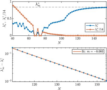
Figure 20: (Color online) Convergence of the extracted real part of the most unstable eigenvalue for the monopole solution for $\mu=20$ as the number of spatial mesh points in increased. We used a domain $(x,y,z)\in[-L_{x},L_{x}]\times[-L_{y},L_{y}]\times[-L_{z},L_{z}]$ where $L_{x}=L_{y}=L_{z}=12$ and discretized it homogeneously along all directions ($dx=dy=dz$) using $N$ points along each direction. The bottom panel depicts the corresponding log-log plot of the data ([blue] circles) for larger values of $N$ and its fit ([orange] line) suggesting that the largest unstable eigenvalue tends to $\lambda^{+}_{\infty}\approx 0.84$ at a rate approximately $\propto 1/N^{8}$.

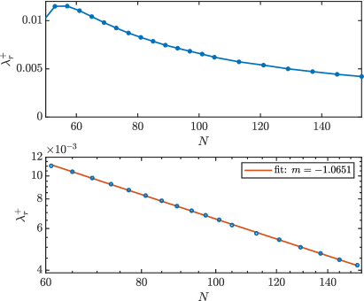
Figure 21: (Color online) Convergence of the numerically (discretization-based) induced instability for the second AR for $\mu=16.5$ as the number of mesh points $N{\mkern-1.0mu\times\mkern-1.0mu}N{\mkern-1.0mu\times\mkern-1.0mu}N$ is increased. In the top panel we depict the largest real part computed from fitting the growth of our FDs+RK4 integration over 1000 (adimensionalized) seconds. The bottom panel depicts the corresponding log-log plot of the data ([blue] circles) for larger values of $N$ and its fit ([orange] line) suggesting that the largest unstable eigenvalue tends to zero at a rate approximately $\propto 1/N$. This suggest that the second AR is indeed stable in the continuum $N\rightarrow\infty$ limit of the actual GP model.

B.2 Eigenvalue computations using forward integrator

The BdG stability problem (see Appendix A) was the most challenging numerical aspect of this work. The idea is to discretize, using FDs, the continuous eigenvalue problem (19). Since large eigenvalue problems are very time and, above all, computer memory intensive, we first studied the convergence of the most unstable mode as a function of the discretization. For this purpose we start with the numerically computed steady state (see above) perturbed by a random perturbation of (relative) size $10^{-10}$ and then integrate forward using our FDs+RK4 integration scheme. By following the norm of the density difference between the evolved state and the initial configuration, we were able to extract (fitting using least squares) the exponential growth of perturbations and thus extract $\lambda^{+}_{r}$, the real part of the most unstable eigenvalue. Figure 20 shows a typical convergence plot of $\lambda^{+}_{r}$ for the monopole solution as the number of mesh points is increased. The bottom panel suggests that the $\lambda^{+}_{r}$ converges to $\lambda^{+}_{\infty}\approx 0.84$ at a rate approximately $\propto 1/N^{8}$. These results indicate that it is necessary to use a relatively large number of mesh points to accurately capture the growth rate associated with the most unstable eigenvalue. Therefore, as a balance between eigenvalue convergence and a manageable system size, we use a computational mesh with $N=129$ for the the monopole spectra results shown in Fig. 16. Given that the monopole solution is generically unstable, we find that the above most-unstable-eigenvalue extraction is practical since, given any initial perturbed stationary state, the instability will eventually develop. However, a more challenging issue arises when the solution is stable (or very weakly unstable) as one needs to integrate for very long times to corroborate that no instability can potentially grow. This, coupled with the issue of needing large meshes to resolve the healing length of the vortex line, quickly results in unmanageable numerics when extracting a BdG stability picture as a function of one or more parameters (in our case the chemical potential $\mu$). This problem is precisely what one faces when trying to determine the stability of the second AR close to its emergence around $\mu=16.35$. Figure 21 depicts the convergence of the computed growth rate for the second AR for $\mu=16.5$ (i.e., slightly to the right of its emergence) as $N$ increases. The top panel indicates that the computed eigenvalue through the FDs+RK4 integration does decrease as $N$ increases. Similar to the convergence of the eigenvalue for the monopole (see Fig. 20), the bottom panel suggests that the second AR eigenvalue tends to zero at an approximate rate $\propto 1/N$. Although this decay rate is weak, it does suggest that the second AR is indeed stable at its inception around $\mu=16.35$. This conclusion is also supported from a bifurcation viewpoint as the first and second ARs seem to be born out of a saddle-center bifurcation and, naturally, one branch must be unstable (first AR) and the other stable (second AR). In fact, we have corroborated (results not shown here) this bifurcation scenario by following the actual BdG spectra for a smaller domain size with $N=35$ using a combination of pseudo-arclength continuation and the eigensolver FEAST (see below). Therefore, we conclude that the second AR is stable in the window $16.35\lesssim\mu\lesssim 19$, namely between its emergence and the appearance of the oscillatory instability bubble.

B.3 BdG eigenvalue and eigenvector computations using eigensolver

It is important to mention that, due to computational limitations, the eigenvectors shown in Figs. 5 and 15 are depicted for $N=51$ and $N=55$ for, respectively, the monopole and AR solutions. For the BdG eigenvalue computations, we used the FEAST eigenvalue algorithm Polizzi (2009); Tang and Polizzi (2014); Kestyn et al. (2016) which combines accuracy, efficiency and robustness even for ill-conditioned matrices (see, for example Charalampidis et al. (2020)). In the present setup, we note that an $N^{3}$ mesh corresponds to a FD BdG stability matrix of size $6N^{3}{\mkern-1.0mu\times\mkern-1.0mu}6N^{3}$ as there are 3 components and the field is complex. The eigenvalue computations were performed on an Intel(R) Core(TM) i7-8700 workstation with 64Gb of RAM. The associated FD stability matrix albeit being highly sparse of size $795,906{\mkern-1.0mu\times\mkern-1.0mu}795,906$ ($998,250{\mkern-1.0mu\times\mkern-1.0mu}998,250$) containing $9,457,236$ ($11,870,100$) non-zero elements for $N=51$ ($N=55$). Therefore, the results depicted in Figs. 5 and 15 should be taken as qualitative rather than quantitative and are hereby presented to help determine the nature of the instabilities experienced by the monopole and AR solutions.

References

- (1)
- Pethick and Smith (2008) C. J. Pethick and H. Smith, Bose-Einstein Condensation in Dilute Gases (Cambridge University Press, Cambridge, United Kingdom, 2008).
- Pitaevskii and Stringari (2018) L. Pitaevskii and S. Stringari, Bose-Einstein Condensation and Superfluidity (Oxford University Press, Oxford, United Kingdom, 2018).
- Stamper-Kurn et al. (1998) D. M. Stamper-Kurn, M. R. Andrews, A. P. Chikkatur, S. Inouye, H.-J. Miesner, J. Stenger, and W. Ketterle, Phys. Rev. Lett. 80, 2027 (1998).
- Stenger et al. (1998) J. Stenger, S. Inouye, D. Stamper-Kurn, H.-J. Miesner, A. Chikkatur, and W. Ketterle, Nature 396, 345 (1998).
- Stamper-Kurn et al. (1999) D. M. Stamper-Kurn, H.-J. Miesner, A. P. Chikkatur, S. Inouye, J. Stenger, and W. Ketterle, Phys. Rev. Lett. 83, 661 (1999).
- Chang et al. (2005) M.-S. Chang, Q. Qin, W. Zhang, L. You, and M. S. Chapman, Nat. Phys. 1, 111 (2005).
- Widera et al. (2006) A. Widera, F. Gerbier, S. Fölling, T. Gericke, O. Mandel, and I. Bloch, New J. Phys. 8, 152 (2006).
- Kawaguchi and Ueda (2012) Y. Kawaguchi and M. Ueda, Physics Reports 520, 253 (2012), ISSN 0370-1573.
- Stamper-Kurn and Ueda (2013) D. M. Stamper-Kurn and M. Ueda, Rev. Mod. Phys. 85, 1191 (2013).
- Kevrekidis and Frantzeskakis (2016) P. G. Kevrekidis and D. J. Frantzeskakis, Rev. Phys. 1, 140 (2016).
- Kevrekidis et al. (2015) P. G. Kevrekidis, D. J. Frantzeskakis, and R. Carretero-González, SIAM, Philadelphia (2015).
- Huh et al. (2020) S. Huh, K. Kim, K. Kwon, and J.-Y. Choi, Phys. Rev. Research 2, 033471 (2020).
- Kim et al. (2021) K. Kim, J. Hur, S. Huh, S. Choi, and J.-y. Choi, arXiv:2102.07613 (2021).
- Li et al. (2005) L. Li, Z. Li, B. A. Malomed, D. Mihalache, and W. Liu, Phys. Rev. A 72, 033611 (2005).
- Zhang et al. (2007) W. Zhang, Ö. Müstecaplıoğlu, and L. You, Phys. Rev. A 75, 043601 (2007).
- Nistazakis et al. (2008) H. Nistazakis, D. Frantzeskakis, P. Kevrekidis, B. Malomed, and R. Carretero-González, Phys. Rev. A 77, 033612 (2008).
- Szankowski et al. (2011) P. Szankowski, M. Trippenbach, and E. Infeld, Eur. Phys. J. D 65, 49 (2011).
- Romero-Ros et al. (2019) A. Romero-Ros, G. Katsimiga, P. Kevrekidis, and P. Schmelcher, Phys. Rev. A 100, 013626 (2019).
- Chai et al. (2020) X. Chai, D. Lao, K. Fujimoto, R. Hamazaki, M. Ueda, and C. Raman, Phys. Rev. Lett. 125, 030402 (2020).
- Chai et al. (2021) X. Chai, D. Lao, K. Fujimoto, and C. Raman, Phys. Rev. Research 3, L012003 (2021).
- Bersano et al. (2018) T. M. Bersano, V. Gokhroo, M. A. Khamehchi, J. D’Ambroise, D. J. Frantzeskakis, P. Engels, and P. G. Kevrekidis, Phys. Rev. Lett. 120, 063202 (2018).
- Fujimoto et al. (2019) K. Fujimoto, R. Hamazaki, and M. Ueda, Phys. Rev. Lett. 122, 173001 (2019).
- Katsimiga et al. (2021) G. C. Katsimiga, S. I. Mistakidis, P. Schmelcher, and P. G. Kevrekidis, New J. Phys. 23, 013015 (2021).
- Lannig et al. (2020) S. Lannig, C.-M. Schmied, M. Prüfer, P. Kunkel, R. Strohmaier, H. Strobel, T. Gasenzer, P. G. Kevrekidis, and M. K. Oberthaler, Phys. Rev. Lett. 125, 170401 (2020).
- Miesner et al. (1999) H.-J. Miesner, D. M. Stamper-Kurn, J. Stenger, S. Inouye, A. Chikkatur, and W. Ketterle, Phys. Rev. Lett. 82, 2228 (1999).
- Świsłocki and Matuszewski (2012) T. Świsłocki and M. Matuszewski, Phys. Rev. A 85, 023601 (2012).
- Ohmi and Machida (1998a) T. Ohmi and K. Machida, J. Phys. Soc. Japan 67, 1822 (1998a).
- Song et al. (2013) S.-W. Song, L. Wen, C.-F. Liu, S.-C. Gou, and W.-M. Liu, Frontiers of Physics 8, 302 (2013).
- Al Khawaja and Stoof (2001) U. Al Khawaja and H. Stoof, Nature 411, 918 (2001).
- Mizushima et al. (2002a) T. Mizushima, K. Machida, and T. Kita, Phys. Rev. Lett. 89, 030401 (2002a).
- Reijnders et al. (2004) J. W. Reijnders, F. J. M. Van Lankvelt, K. Schoutens, and N. Read, Phys. Rev. A 69, 023612 (2004).
- Mizushima et al. (2002b) T. Mizushima, K. Machida, and T. Kita, Phys. Rev. A 66, 053610 (2002b).
- Leslie et al. (2009) L. S. Leslie, A. Hansen, K. C. Wright, B. M. Deutsch, and N. P. Bigelow, Phys. Rev. Lett. 103, 250401 (2009).
- Hall et al. (2016) D. S. Hall, M. W. Ray, K. Tiurev, E. Ruokokoski, A. H. Gheorghe, and M. Möttönen, Nat. Phys. 12, 478 (2016).
- Lee et al. (2018) W. Lee, A. H. Gheorghe, K. Tiurev, T. Ollikainen, M. Möttönen, and D. S. Hall, Science Advances 4 (2018).
- Stoof et al. (2001) H. T. C. Stoof, E. Vliegen, and U. Al Khawaja, Phys. Rev. Lett. 87, 120407 (2001).
- Ray et al. (2015) M. W. Ray, E. Ruokokoski, K. Tiurev, M. Möttönen, and D. S. Hall, Science 348, 544 (2015).
- Ollikainen et al. (2017) T. Ollikainen, K. Tiurev, A. Blinova, W. Lee, D. S. Hall, and M. Möttönen, Phys. Rev. X 7, 021023 (2017).
- Ruostekoski and Anglin (2003) J. Ruostekoski and J. R. Anglin, Phys. Rev. Lett. 91, 190402 (2003).
- Tiurev et al. (2016) K. Tiurev, E. Ruokokoski, H. Mäkelaä, D. S. Hall, and M. Möttönen, Phys. Rev. A 93, 033638 (2016).
- Robins et al. (2001) N. P. Robins, W. Zhang, E. A. Ostrovskaya, and Y. S. Kivshar, Phys. Rev. A 64, 021601 (2001).
- Ohmi and Machida (1998b) T. Ohmi and K. Machida, Journal of the Physical Society of Japan 67, 1822 (1998b).
- Ho (1998) T.-L. Ho, Phys. Rev. Lett. 81, 742 (1998).
- Manakov (1974) S. V. Manakov, Sov. Phys. JETP 38, 248 (1974).
- Leanhardt et al. (2003) A. E. Leanhardt, Y. Shin, D. Kielpinski, D. E. Pritchard, and W. Ketterle, Phys. Rev. Lett. 90, 140403 (2003).
- Black et al. (2007) A. T. Black, E. Gomez, L. D. Turner, S. Jung, and P. D. Lett, Phys. Rev. Lett. 99, 070403 (2007).
- Samuelis et al. (2000) C. Samuelis, E. Tiesinga, T. Laue, M. Elbs, H. Knöckel, and E. Tiemann, Phys. Rev. A 63, 012710 (2000).
- Pietilä and Möttönen (2009) V. Pietilä and M. Möttönen, Phys. Rev. Lett. 103, 030401 (2009).
- Mueller (2004) E. J. Mueller, Phys. Rev. A 69, 033606 (2004).
- Symes and Blakie (2017) L. M. Symes and P. B. Blakie, Phys. Rev. A 96, 013602 (2017).
- Feder et al. (2000) D. L. Feder, M. S. Pindzola, L. A. Collins, B. I. Schneider, and C. W. Clark, Phys. Rev. A 62, 053606 (2000).
- Charalampidis et al. (2016) E. G. Charalampidis, W. Wang, P. G. Kevrekidis, D. J. Frantzeskakis, and J. Cuevas-Maraver, Phys. Rev. A 93, 063623 (2016).
- Doedel and Tuckerman (2000) E. Doedel and L. S. Tuckerman, Numerical Methods for Bifurcation Problems and Large-Scale Dynamical Systems (Springer-Verlag, Heidelberg, Germany, 2000).
- Kelley (2003) C. T. Kelley, Solving Nonlinear Equations with Newton’s Method (SIAM, 2003).
- Caplan and Carretero-González (2013) R. M. Caplan and R. Carretero-González, App. Num. Math. 71, 24 (2013).
- Polizzi (2009) E. Polizzi, Phys. Rev. B 79, 115112 (2009).
- Tang and Polizzi (2014) P. T. P. Tang and E. Polizzi, SIAM J. Matrix Anal. Appl. 35, 354 (2014).
- Kestyn et al. (2016) J. Kestyn, E. Polizzi, and P. T. P. Tang, SIAM J. Sci. Comp. 38, S772 (2016).
- Charalampidis et al. (2020) E. G. Charalampidis, N. Boullé, P. E. Farrell, and P. G. Kevrekidis, Comm. Nonlin. Sci. and Numer. Simulat. 87, 105255 (2020), ISSN 1007-5704.