3HDM with $\Delta(27)$ symmetry and its phenomenological consequences

Abstract

We perform a comprehensive analysis of a version of the 3-Higgs doublet model whose scalar potential is invariant under a global $\Delta(27)$ discrete symmetry and where the three scalar doublets are chosen to transform as a triplet under this discrete group. For each of the known tree-level minima we study the mass spectra and use the oblique parameters $STU$ as well as perturbative unitarity to constrain the parameter space of the model. We then discuss phenomenological consequences of some leading order flavour mixing quark Yukawa couplings by considering the flavour violation process $b\to s\gamma$.

We show that perturbative unitarity significantly constrains parameters of the model while, conversely, the beyond the Standard Model contributions to the $b\to s\gamma$ decay are automatically tamed by the symmetry.

CERN-TH-2021-182

1 Introduction

The discovery of the Higgs boson and the (so far) non-observation of new particles at the LHC have confirmed the Standard Model as our paradigm. Only the observation of neutrino mixing requires its extension in the leptonic sector. However, a number of theoretical arguments as well as experimental observations still motivate searches for a more fundamental theory. Extensions of the scalar sector of the Standard Model (SM) are particularly well motivated. One of the simplest ones is the well-known two-Higgs doublet model (2HDM) which, in its different incarnations, has been already extensively studied (see for example Gunion:1989we ; Branco:2011iw ). Models with more Higgs doublets transforming non-trivially under non-Abelian discrete symmetries have also gained interest, in particular in the context of predicting the observed mixing patterns of leptons or quarks. That is because, in its most general form, already a three-Higgs doublet model (3HDM) has a large number of free parameters in the scalar sector alone. Therefore it is particularly appealing from the point of view of model building to impose additional symmetries in the scalar sector. Symmetries play an important role in reducing the number of free parameters and, as a result, they increase the predictive power of the model. Continuous symmetries, when spontaneously broken, lead to undesired massless Goldstone bosons. There is however a small list of finite symmetries a 3HDM can possess without having also a continuous symmetry Ivanov:2012fp (see also Darvishi:2019dbh ; Darvishi:2021txa ). Among the more predictive potentials are those where the 3 Higgs fields transform as a triplet of a non-Abelian discrete symmetry. The highlights of these cases are the $A_{4}$ and $\Delta(27)$ symmetries.

The phenomenology of the $A_{4}$ invariant potential has been analysed in detail already several years ago Toorop:2010ex ; Toorop:2010kt . Meanwhile, while the $\Delta(27)$ symmetry has been often used in particle physics, it was usually done so in a slightly different context (e.g. Branco:1983tn ; deMedeirosVarzielas:2006fc ; Ma:2006ip ; deMedeirosVarzielas:2011zw ; Varzielas:2012nn ; Bhattacharyya:2012pi ; Ferreira:2012ri ; Ma:2013xqa ; Nishi:2013jqa ; Varzielas:2013sla ; Aranda:2013gga ; Varzielas:2013eta ; Harrison:2014jqa ; Ma:2014eka ; Fallbacher:2015rea ; Abbas:2015zna ; Varzielas:2015aua ; Bjorkeroth:2015uou ; Chen:2015jta ; Hernandez:2016eod ; CarcamoHernandez:2017owh ; deMedeirosVarzielas:2017sdv ; Bernal:2017xat ; deMedeirosVarzielas:2018vab ; CarcamoHernandez:2018djj ; Bjorkeroth:2019csz ). Namely, an interesting feature of a model with such a symmetry is that it exhibits Geometrical CP Violation Branco:1983tn ; deMedeirosVarzielas:2011zw ; Varzielas:2012nn ; Bhattacharyya:2012pi ; Ma:2013xqa ; Nishi:2013jqa ; Varzielas:2013sla ; Varzielas:2013eta ; Fallbacher:2015rea , which means that there are minima of the potential that violate CP independently of the parameters of the potential, their form being fixed by the symmetry.

In this paper we therefore aim to fill this gap, by performing a thorough phenomenological analysis of the $\Delta(27)$ invariant potential (with a $\Delta(27)$ triplet of $SU(2)_{L}$ doublets), which in fact coincides with the $\Delta(54)$ invariant potential for the same field content. We refer throughout this work to it as the $\Delta(27)$ potential as we assign fermions also to $\Delta(27)$ representations to study leading order in terms of flavour mixing Yukawa structures and associated flavour violating processes.

We perform an analysis analogous to the study done for the $A_{4}$ potential in Toorop:2010ex ; Toorop:2010kt . Namely, we investigate how the parameter space of this potential becomes constrained by $STU$ parameters, perturbative unitarity and, when considering Yukawa structures, the $b\to s\gamma$ process.

In Section 2 we describe the model in detail, covering regions of parameter space, possible minima and relations between the physical parameters (masses etc.) and the parameters of the potential. We also discuss possible leading order extensions of the model to the fermion sector for each minimum. As mentioned before, we extend the model to the fermionic sector by choosing how the fermions transform under the $\Delta(27)$ symmetry, thus determining the structure of the Yukawa couplings. Although realistic fermion mixing requires further symmetry breaking, nevertheless even in this simple implementation we can already discuss some important features such as the leading aspects of the Higgs mediated flavour changing neutral currents.

In Section 3 we present the constraints from $STU$ and unitarity in terms of physical masses of the charged and neutral Higgs bosons. Finally, we conclude in Section 4.

Appendix A contains the relevant details on the discrete group $\Delta(27)$, while Appendix B gives some technical details on SPheno setup and calculation of unitarity constraints. We also give an example of non-SM Higgs decays pattern in Appendix C.

2 The $\Delta(27)$ symmetric 3HDM

In this section we discuss the scalar potential, its tree-level minima, Higgs mass matrices as well as the fermion sector of the model.

We consider the most general CP-conserving 3HDM scalar potential, where the Higgs field content is a triplet of $\Delta(27)$ in which each of the three components of the triplet is an $SU(2)_{L}$ doublet. For phenomenological analysis the model is encoded into SARAH Staub:2009bi ; Staub:2010jh ; Staub:2012pb ; Staub:2013tta version 4.14.5 which, among others, automatically derives aforementioned mass matrices and tadpole equations (minima conditions), as well as interaction vertices.

2.1 Scalar potential

Using the notation as in Varzielas:2016zjc ; deMedeirosVarzielas:2017glw , the scalar potential has a contribution that is common to all $\Delta(3n^{2})$ ($n\geq 3$) potentials

$$V_{0}(\Phi)= -\mu^{2}\sum_{i,\alpha}\Phi_{i\alpha}\Phi^{*i\alpha}+s\sum_{i,\alpha,\beta}(\Phi_{i\alpha}\Phi^{*i\alpha})(\Phi_{i\beta}\Phi^{*i\beta})$$

$$+\sum_{i,j,\alpha,\beta}\left[r_{1}(\Phi_{i\alpha}\Phi^{*i\alpha})(\Phi_{j\beta}\Phi^{*j\beta})+r_{2}(\Phi_{i\alpha}\Phi^{*i\beta})(\Phi_{j\beta}\Phi^{*j\alpha})\right],$$ (1)

where the index $i=1,2,3$ refers to the doublet and $\alpha,\beta=1,2$ to the $SU(2)_{L}$ component of the doublet, either up or down. $\Delta(3n^{2})$ ($n\geq 3$) is a discrete subgroup of the continuous $SU(3)$ group (not to be confused with the $SU(3)_{C}$ gauge symmetry of the SM), and $V_{0}$ would be invariant under the continuous $SU(3)$ if the coefficient $s$ was set to zero. The potential that is invariant under $\Delta(27)$ ($\Delta(3n^{2})$ with $n=3$) contains $V_{0}$ and in addition the following term

$$V_{\Delta(27)}(\Phi)=V_{\Delta(54)}(\Phi)=V_{0}(\Phi)~{}+~{}\sum_{\alpha,\beta}\left[d\left(\Phi_{1\alpha}\Phi_{1\beta}\Phi^{*2\alpha}\Phi^{*3\beta}+\text{cycl.}\right)+\text{h.c.}\right],$$ (2)

which is not invariant under $A_{4}$ or $\Delta(3n^{2})$ for $n>3$ but still coincides with the $\Delta(54)$ potential. Only when we extend the model to the fermionic sector and choose how the fermions transform under the symmetry, thus determining the structure of the Yukawa couplings, will it be possible to distinguish the two types of models. The parameter $d$ in Eq. (2) is the only parameter of the potential that can be complex. Choosing $d$ to be real (as we do in this work) leads to a explicit CP-conserving potential and it allows for a simple CP transformation under which each doublet transforms trivially, i.e. each doublet transforms into its complex conjugate. We note that CP can also be conserved with a complex $d$ provided that its phase is of the form $\pm i\tfrac{2\pi}{3}$. In the latter case the CP transformation is no longer the trivial one and will relate different doublets and their complex conjugates. The potential (2) has the interesting feature of having minima with spontaneous geometrical CP violation Branco:1983tn ; deMedeirosVarzielas:2011zw for real $d$, i.e., for a large region of parameter space there is a CP violating minimum where the phases of the vacuum expectation value (VEV) are fixed to a specific value (in this case, an integer multiple of $2\pi/3$), with this value not depending on the parameters of the potential (however, for sufficiently large variation of the parameters, one gets into a separate region of parameter space, where the minima belong to a different class).

2.2 The minima of the potential

After spontaneous gauge symmetry breakdown the Higgs doublets can be decomposed as

$$\Phi_{j}=e^{i\alpha_{j}}\left(\begin{array}[]{c}\phi^{+}_{j}\\ \frac{1}{\sqrt{2}}(v_{j}+ia_{j}+\rho_{j}+i\eta_{j})\end{array}\right),\qquad j=1,2,3$$ (5)

with real scalar fields $\rho_{j}$, $\eta_{j}$ and $v_{j}+ia_{j}$ the (complex) vacuum expectation values (where $v_{i}$ and $a_{i}$ are real numbers).

The minima of the potential (2) have been classified previously Ivanov:2014doa ; deMedeirosVarzielas:2017glw . As discussed above, the real parameter $s$ governs a term that is not $SU(3)$ invariant and that distinguishes directions of VEVs. For $s<0$, the global minimum favoured is in the $(v,0,0)$ direction, while for $s>0$ in the $(v,v,v)/\sqrt{3}$ direction. The $d$ parameter (complex in general) governs the phase-dependent term that makes the potential invariant under $\Delta(27)$ (or $\Delta(54)$ to be more precise). If the magnitude of this coefficient is large it disfavours $(v,0,0)$ being the global minimum, as for this VEV $d$ does not contribute to the potential — a direction like $(v,v,v)/\sqrt{3}$ or $(\omega v,v,v)/\sqrt{3}$ or similar becomes the global minimum when $d$ dominates ($\omega\equiv\exp(2\pi i/3$)). Then, if a CP symmetry is imposed making $d$ a real parameter, the sign of $d$ determines the class of the minima, for positive $d$ the minimum is of the class $(\omega v,v,v)/\sqrt{3}$, with spontaneous geometrical CP violation.

2.2.1 General VEVs $v_{i}+ia_{i}$

Here we list the extrema conditions for completely general complex VEVs

$$\frac{\partial V}{\partial v_{1}}= -\mu^{2}v_{1}+sv_{1}(v_{1}^{2}+a_{1}^{2})+(r_{1}+r_{2})v_{1}(v_{1}^{2}+a_{1}^{2}+v_{2}^{2}+a_{2}^{2}+v_{3}^{2}+a_{3}^{2})$$ (6)

$$+d[v_{1}(v_{2}v_{3}-a_{2}a_{3})+v_{2}a_{3}(a_{1}+a_{2})+a_{2}v_{3}(a_{1}+a_{3})+\tfrac{1}{2}v_{2}(v^{2}_{3}-a^{2}_{3})+\tfrac{1}{2}v_{3}(v_{2}^{2}-a_{2}^{2})],$$

$$\frac{\partial V}{\partial a_{1}}= -\mu^{2}a_{1}+sa_{1}(v_{1}^{2}+a_{1}^{2})+(r_{1}+r_{2})a_{1}(v_{1}^{2}+a_{1}^{2}+v_{2}^{2}+a_{2}^{2}+v_{3}^{2}+a_{3}^{2})$$ (7)

$$+d[a_{1}(a_{2}a_{3}-v_{2}v_{3})+v_{2}a_{3}(v_{1}+v_{3})+a_{2}v_{3}(v_{1}+v_{2})+\tfrac{1}{2}a_{2}(a_{3}^{2}-v_{3}^{2})+\tfrac{1}{2}a_{3}(a_{2}^{2}-v_{2}^{2})]$$

and the other 4 eqs. obtained by a cyclic permutation of $(123)$.

The above equations are simplified when considering real VEVs. Then we have as equations

$$\tfrac{1}{2}dv_{1}v_{2}(v_{1}+v_{2}+2v_{3})+v_{3}(-\mu^{2}+sv_{3}^{2}+(r_{1}+r_{2})(v_{1}^{2}+v_{2}^{2}+v_{3}^{2}))=0$$ (8)

plus two cyclic permutations. We found several solutions to these equations, which we separate depending on whether their direction does or does not depend directly on the parameters of the potential. Within the solutions we find the (known) minima: $(v,0,0)$ and $(v,v,v)$, as well as solutions of the type $(v,-v,0)$ which we verified analytically can not be minima for any region of parameter space. There are also solutions, whose entries are complicated functions of the parameters, which we checked numerically are not minima for any of the points in parameter space we sampled. This is in agreement with Ivanov:2014doa ; deMedeirosVarzielas:2017glw . For complex VEVs we relied on the known solutions $(\omega v,v,v)$ and $(\omega^{2}v,v,v)$ (and cyclic permutations) Ivanov:2014doa ; deMedeirosVarzielas:2017glw . As we are considering cases with CP symmetry of the potential, $(\omega^{2}v,v,v)$ is related by the CP symmetry to $(\omega v,v,v)$, so we do not need to consider it separately.

2.2.2 The $(v,0,0)$ case

To be a minimum the region of parameter space for $(v,0,0)$ requires

$$\mu^{2}=(r_{1}+r_{2}+s)v^{2}.$$ (9)

In this case the $\Phi_{1}$ plays the role of the SM Higgs doublet, while the other two doublets remain VEV-less and couple to gauge bosons only through quartic couplings even after the Electroweak Symmetry Breaking (EWSB). Therefore we identify $v$ with the SM VEV, $v\approx 247$ GeV. The CP-even Higgs mass matrix takes the form

$$m_{H}^{2}=\begin{pmatrix}2(r_{1}+r_{2}+s)&0&0\\ 0&-s&\tfrac{1}{2}d\\ 0&\tfrac{1}{2}d&-s\end{pmatrix}v^{2}$$ (10)

with eigenvalues $m_{h}^{2}=2(r_{1}+r_{2}+s)v^{2}$, $m^{2}_{H_{1}}=\tfrac{1}{2}(d-2s)v^{2}$, $m^{2}_{H_{2}}=-\tfrac{1}{2}(d+2s)v^{2}$, where $m_{H_{1}}$ and $m_{H_{2}}$ are not mass ordered, and $h$ is to be identified with the SM-like Higgs.

The CP-odd Higgs mass matrix is given by

$$m_{A}^{2}=\begin{pmatrix}0&0&0\\ 0&-s&-\tfrac{1}{2}d\\ 0&-\tfrac{1}{2}d&-s\end{pmatrix}v^{2}+\text{gauge dependent terms}$$ (11)

with eigenvalues $m_{A_{1}}^{2}=\tfrac{1}{2}(d-2s)v^{2}$, $m_{A_{2}}^{2}=-\tfrac{1}{2}(d+2s)v^{2}$ and a Goldstone boson $G^{0}$. The $m_{H^{\pm}}^{2}$ matrix is diagonal, with $m_{H^{\pm}_{1}}^{2}=m_{H^{\pm}_{2}}^{2}=-(r_{2}+s)v^{2}$ and a Goldstone boson $G^{\pm}$.

The Lagrangian parameters can be expressed in terms of physical masses of Higgses as

$$s= -\frac{1}{2v^{2}}(m_{H_{1}}^{2}+m_{H_{2}}^{2}),$$ (12)

$$r_{1}= \mathbin{\hphantom{-}}\frac{1}{2v^{2}}(m_{h}^{2}+2m_{H^{\pm}}^{2}),$$ (13)

$$r_{2}= \mathbin{\hphantom{-}}\frac{1}{2v^{2}}(m_{H_{1}}^{2}+m_{H_{2}}^{2}-2m_{H^{\pm}}^{2}),$$ (14)

$$d= \mathbin{\hphantom{-}}\frac{1}{v^{2}}(m_{H_{1}}^{2}-m_{H_{2}}^{2}).$$ (15)

Here $H^{\pm}$ is a simplified notation for either $H^{\pm}_{1}$ or $H^{\pm}_{2}$, which are degenerate in mass. Likewise $A_{i}$ are pairwise mass degenerate with $H_{i}$.

2.2.3 The $(v,v,v)$ case

To be a minimum the region of parameter space for $(v,v,v)$ requires

$$\mu^{2}=(2d+3r_{1}+3r_{2}+s)v^{2}.$$ (16)

The CP-even Higgs mass matrix takes the form $(r_{12}\equiv r_{1}+r_{2})$

$$m_{H}^{2}=\frac{1}{2}\begin{pmatrix}4(r_{12}+s)-2d&5d+4r_{12}&5d+4r_{12}\\ 5d+4r_{12}&4(r_{12}+s)-2d&5d+4r_{12}\\ 5d+4r_{12}&5d+4r_{12}&4(r_{12}+s)-2d\end{pmatrix}v^{2}$$ (17)

with eigenvalues $m_{h}^{2}=2(2d+3r_{12}+s)v^{2}$ (to be identified with the SM-like Higgs boson mass) and $m_{H}^{2}=1/2(-7d+4s)v^{2}$ (the mass of the pair of degenerate Higgs bosons $H_{1}$ and $H_{2}$).

The CP-odd mass matrix is given by

$$m_{A}^{2}=\frac{3}{2}\begin{pmatrix}-2&1&1\\ 1&-2&1\\ 1&1&-2\\ \end{pmatrix}dv^{2}+\text{gauge dependent terms}.$$ (18)

The two physical CP-odd Higgs bosons $A_{1}$ and $A_{2}$ are mass degenerate with a common mass $m_{A}^{2}=-9dv^{2}/2$. Similarly the charged Higgs bosons mass matrix is given by

$$m_{H^{\pm}}^{2}=\begin{pmatrix}-2&1&1\\ 1&-2&1\\ 1&1&-2\\ \end{pmatrix}(r_{2}+d)v^{2}+\text{gauge dependent terms},$$ (19)

where $H_{1}^{\pm}$ and $H_{2}^{\pm}$ are also mass degenerate, with a common mass $m_{H^{\pm}}^{2}=-3(d+r_{2})v^{2}$.

The Lagrangian parameters can be expressed in terms of physical masses of Higgses as

$$s= \mathbin{\hphantom{-}}\frac{1}{18v^{2}}(9m_{H}^{2}-7m_{A}^{2}),$$ (20)

$$r_{1}= \mathbin{\hphantom{-}}\frac{1}{18v^{2}}(m_{A}^{2}+6m_{H^{\pm}}^{2}+3m_{h}^{2}-3m_{H}^{2}),$$ (21)

$$r_{2}= \mathbin{\hphantom{-}}\frac{1}{9v^{2}}(2m_{A}^{2}-3m_{H^{\pm}}^{2}),$$ (22)

$$d= -\frac{2}{9v^{2}}m_{A}^{2}.$$ (23)

2.2.4 The $(\omega v,v,v)$ case

To be a minimum the region of parameter space for $(\omega v,v,v)$ requires

$$\mu^{2}= (-d+3r_{12}+s)v^{2}.$$ (24)

Because in this vacuum CP is spontaneously broken, this time all Higgs bosons mix and the mass matrix for the neutral ones takes the form

$$m_{H}^{2}=\begin{pmatrix}m_{HH}^{2}&m_{HA}^{2}\\ (m_{HA}^{2})^{T}&m_{AA}^{2}\end{pmatrix}v^{2}+\text{gauge dependent terms},$$ (25)

where the 3x3 submatrices are as follows

$$m_{HH}^{2}= \begin{pmatrix}\frac{1}{2}\left(4d+r_{12}+s\right)&d-r_{12}&d-r_{12}\\ d-r_{12}&\frac{1}{2}\left(d+4\left(r_{12}+s\right)\right)&\frac{1}{4}\left(8r_{12}-5d\right)\\ d-r_{12}&\frac{1}{4}\left(8r_{12}-5d\right)&\frac{1}{2}\left(d+4\left(r_{12}+s\right)\right)\end{pmatrix},$$ (26)

$$m_{HA}^{2}= \frac{\sqrt{3}}{2}\begin{pmatrix}-\left(r_{12}+s\right)&-d+2r_{12}&-d+2r_{12}\\ d&d&-d/2\\ d&-d/2&d\end{pmatrix},$$ (27)

$$m_{AA}^{2}= \frac{3}{2}\begin{pmatrix}r_{12}+s&0&0\\ 0&d&-d/2\\ 0&-d/2&d\end{pmatrix}$$ (28)

with the eigenvalues

$$m_{h}^{2} =2v^{2}\left(-d+3r_{1}+3r_{2}+s\right),$$ (29)

$$m_{H_{1}}^{2} =m_{H_{2}}^{2}=\frac{1}{2}\left(4d+2s-\sqrt{7d^{2}-2ds+4s^{2}}\right)v^{2},$$ (30)

$$m_{H_{3}}^{2} =m_{H_{4}}^{2}=\frac{1}{2}\left(4d+2s+\sqrt{7d^{2}-2ds+4s^{2}}\right)v^{2}.$$ (31)

We assume that the single mass-nondegenerate state $h$ is identified with the SM-like Higgs.

The mass matrix for the charged Higgs bosons reads

$$m_{H^{-}H^{+}}^{2}=(d-2r_{2})\begin{pmatrix}1&-\tfrac{\omega}{2}&-\tfrac{\omega}{2}\\ -\frac{\omega^{*}}{2}\ &1&-\tfrac{1}{2}\\ -\tfrac{\omega^{*}}{2}&-\tfrac{1}{2}&1\end{pmatrix}v^{2}+\text{gauge dependent terms}.$$ (32)

Physical charged states are mass degenerate, with mass $m_{H^{\pm}_{1}}^{2}=m_{H^{\pm}_{2}}^{2}=\frac{3}{2}(d-2r_{2})v^{2}$ .

Because of the quadratic nature of expressions for masses $m_{H_{i}}^{2}$ there are two combinations of potential parameters that give the same 4 masses $m_{h}$, $m_{H_{1}}$, $m_{H_{3}}$ and $m_{H^{\pm}}$, namely

$$s= \frac{1}{18v^{2}}\left(3m_{H_{1}}^{2}+3m_{H_{3}}^{2}\mp 2\Omega\right),$$ (33)

$$r_{1}= \frac{1}{18v^{2}}\left(6m_{h}^{2}-3m_{H_{1}}^{2}-3m_{H_{3}}^{2}+12m_{H^{\pm}}^{2}\pm\Omega\right),$$ (34)

$$r_{2}= \frac{1}{18v^{2}}\left(3m_{H_{1}}^{2}+3m_{H_{3}}^{2}-12m_{H^{\pm}}^{2}\pm\Omega\right),$$ (35)

$$d= \frac{1}{18v^{2}}\left(3m_{H_{1}}^{2}+3m_{H_{3}}^{2}\pm\Omega\right),$$ (36)

where $m_{H_{3}}^{2}>3m_{H_{1}}^{2}$ in order for $\Omega\equiv\sqrt{9m_{H_{1}}^{4}-30m_{H_{1}}^{2}m_{H_{3}}^{2}+9m_{H_{3}}^{4}}$ to be real.

2.3 Yukawa couplings

Having discussed the scalar potential and its vacua, we now proceed with description of the Yukawa interactions.

The general form of the quark Yukawa couplings in models with three Higgs doublets is

$$L_{Y}= -\overline{Q_{L}}\ \Gamma_{1}\Phi_{1}d_{R}-\overline{Q_{L}}\ \Gamma_{2}\Phi_{2}d_{R}-\overline{Q_{L}}\ \Gamma_{3}\Phi_{3}d_{R}$$

$$-\overline{Q_{L}}\ \Delta_{1}\tilde{\Phi}_{1}u_{R}-\overline{Q_{L}}\ \Delta_{2}\tilde{\Phi}_{2}u_{R}\ -\overline{Q_{L}}\ \Delta_{3}\tilde{\Phi}_{3}u_{R}\ +\mbox{h.c.},$$ (37)

where $\Gamma_{i}$ and $\Delta_{i}$ denote the Yukawa couplings of the left-handed (LH) quark doublets $Q_{L}$ to the Higgs doublets $\Phi_{j}$ and, respectively, right-handed (RH) quarks $d_{R}$ or $u_{R}$. After spontaneous symmetry breaking quark mass matrices are generated with the form

$$M_{d} = \frac{1}{\sqrt{2}}(v_{1}e^{i\alpha_{1}}\Gamma_{1}+v_{2}e^{i\alpha_{2}}\Gamma_{2}+v_{3}e^{i\alpha_{3}}\Gamma_{3}),$$

$$M_{u} = \frac{1}{\sqrt{2}}(v_{1}e^{-i\alpha_{1}}\Delta_{1}+v_{2}e^{-i\alpha_{2}}\Delta_{2}+v_{3}e^{-i\alpha_{3}}\Delta_{3}).$$ (38)

The matrices $M_{d},M_{u}$ are then diagonalised by the usual bi-unitary transformations

$$U^{\dagger}_{dL}M_{d}U_{dR}=D_{d}\equiv{\mbox{d}iag}\ (m_{d},m_{s},m_{b}),$$ (39)

$$U^{\dagger}_{uL}M_{u}U_{uR}=D_{u}\equiv{\mbox{d}iag}\ (m_{u},m_{c},m_{t}).$$ (40)

Before we can continue with the phenomenological analysis we need to assign the fermions to $\Delta(27)$ representations to obtain semi-realistic Yukawa couplings. The RH quarks we choose to be $\Delta(27)$ triplets because, as we present in more detail for each of the VEVs, this choice allows us to make semi-realistic $\Delta(27)$ invariants for both up and down quark sectors. The 3 LH quark doublets will be distinct $\Delta(27)$ singlets but the choice of representations depends on the VEV, in order to have Yukawa structures that are realistic at leading order - we are able to obtain distinct masses for each generation but with a CKM matrix that is the unit matrix, which is a consequence of breaking $\Delta(27)$ with just one triplet scalar that leaves too much residual unbroken flavour symmetry. While such mixing angles are clearly not viable, we consider this to be a good leading-order approximation. We consider these Yukawa structures as toy models to obtain constraints on the scalar sector. More realistic mixing angles can be obtained by adding further sources of $\Delta(27)$ breaking Bhattacharyya:2012pi ; Varzielas:2013sla ; Varzielas:2013eta .

In the following subsections we present Yukawa couplings as $Y_{u}$, $Y_{d}$ and $Y_{e}$ matrices, and later show the respective $\Gamma$, $\Delta$ matrices that couple to each of the $\Phi_{i}$ fields.

2.3.1 The $(v,0,0)$ case

For the simplest VEV, the choice of singlets is one trivial ($1_{00}$) and two non-trivial $1_{0i}$ ($i=1,2$). This choice corresponds to having the three singlets that do not transform under the generator $c$ of $\Delta(27)$ (see Appendix A), such that we have the desired composition rules from the product of the (anti-)triplet RH quark (either $d_{R}$ or $u_{R}$) and the (anti-)triplet Higgs (either $\Phi_{j}$ for the down sector or its conjugate for the up sector).

In particular, with $(d_{R})_{i}$ ($i=1\ldots 3$, the generation index) transforming as an anti-triplet $\bar{3}$, the $\Delta(27)$ invariant terms are then of the type $\bar{Q}_{i}(\Phi d_{R})_{0j}$, whereas $(u_{R})_{i}$ should transform as a triplet $3$ to construct similarly the invariants with $\tilde{\Phi}$ which transforms as an anti-triplet $\bar{3}$, i.e. $\bar{Q}_{i}(u_{R}\tilde{\Phi})_{0j}$.

For $\bar{Q}_{1},\bar{Q}_{2},\bar{Q}_{3}$ belonging to, respectively, $1_{00},1_{02}$ and $1_{01}$ the corresponding Yukawa terms are

$$L_{Y}^{d}=\bar{Q}Y_{d}d_{R}\equiv y_{1}^{d}\bar{Q}_{1}\left(\Phi_{1}(d_{R})_{1}+\Phi_{2}(d_{R})_{2}+\Phi_{3}(d_{R})_{3}\right)_{00}+$$

$$y_{2}^{d}\bar{Q}_{2}\left(\Phi_{3}(d_{R})_{1}+\Phi_{1}(d_{R})_{2}+\Phi_{2}(d_{R})_{3}\right)_{01}+$$

$$y_{3}^{d}\bar{Q}_{3}\left(\Phi_{2}(d_{R})_{1}+\Phi_{3}(d_{R})_{2}+\Phi_{1}(d_{R})_{3}\right)_{02}.$$ (41)

These expressions follow from the specific choice of non-trivial singlets made for the LH quarks and the composition rules of $\Delta(27)$ listed in Appendix A.

The Yukawa terms above correspond to Yukawa matrices of the form (in LR convention)

$$Y_{d}=\begin{pmatrix}y_{1}^{d}\Phi_{1}&y_{1}^{d}\Phi_{2}&y_{1}^{d}\Phi_{3}\\ y_{2}^{d}\Phi_{3}&y_{2}^{d}\Phi_{1}&y_{2}^{d}\Phi_{2}\\ y_{3}^{d}\Phi_{2}&y_{3}^{d}\Phi_{3}&y_{3}^{d}\Phi_{1}\end{pmatrix}.$$ (42)

The mass matrices are now easy to read of when $\Phi$ acquires its VEV, breaking $SU(2)_{L}$ and $\Delta(27)$. In this subsection we are dealing with the $(v,0,0)$ VEV, which means that we are already in the Higgs basis. The down quark mass matrix then looks as follows

$$M_{d}=\begin{pmatrix}y_{1}^{d}v&0&0\\ 0&y_{2}^{d}v&0\\ 0&0&y_{3}^{d}v\end{pmatrix}.$$ (43)

Because the LH quarks are $\Delta(27)$ singlets, it is easy to adapt the above assignments to the up quark sector giving

$$L_{Y}^{u}= y_{1}^{u}\bar{Q}_{1}\left(\tilde{\Phi}_{1}(u_{R})_{1}+\tilde{\Phi}_{2}(u_{R})_{2}+\tilde{\Phi}_{3}(u_{R})_{3}\right)_{00}+$$

$$y_{2}^{u}\bar{Q}_{2}\left(\tilde{\Phi}_{2}(u_{R})_{1}+\tilde{\Phi}_{3}(u_{R})_{2}+\tilde{\Phi}_{1}(u_{R})_{3}\right)_{01}+$$

$$y_{3}^{u}\bar{Q}_{3}\left(\tilde{\Phi}_{3}(u_{R})_{1}+\tilde{\Phi}_{1}(u_{R})_{2}+\tilde{\Phi}_{2}(u_{R})_{3}\right)_{02}.$$ (44)

Note the change compared to the down sector. We have to construct the same singlets of $\Delta(27)$ from $3\times\bar{3}$ (see Appendix A), but in the down sector the scalar $\Phi$ is in the $3$ and the RH fermion is in the $\bar{3}$, whereas in the up sector the scalar $\tilde{\Phi}$ is in the $\bar{3}$ and it is the RH fermion that transforms as $3$. Thus

$$Y_{u}=\begin{pmatrix}y_{1}^{u}\tilde{\Phi}_{1}&y_{1}^{u}\tilde{\Phi}_{2}&y_{1}^{u}\tilde{\Phi}_{3}\\ y_{2}^{u}\tilde{\Phi}_{2}&y_{2}^{u}\tilde{\Phi}_{3}&y_{2}^{u}\tilde{\Phi}_{1}\\ y_{3}^{u}\tilde{\Phi}_{3}&y_{3}^{u}\tilde{\Phi}_{1}&y_{3}^{u}\tilde{\Phi}_{2}\end{pmatrix}.$$ (45)

For the $(v,0,0)$ VEV we therefore have

$$M_{u}=\begin{pmatrix}y_{1}^{u}v&0&0\\ 0&0&y_{2}^{u}v\\ 0&y_{3}^{u}v&0\end{pmatrix},$$ (46)

which gives

$$M_{u}M_{u}^{\dagger}=\begin{pmatrix}|y_{1}^{u}v|^{2}&0&0\\ 0&|y_{2}^{u}v|^{2}&0\\ 0&0&|y_{3}^{u}v|^{2}\end{pmatrix}.$$ (47)

Given that both $M_{u}M_{u}^{\dagger}$ and $M_{d}M_{d}^{\dagger}$ are diagonal, the CKM matrix in this limit is the identity matrix. For this phenomenological study we consider this as a reasonable leading order approximation.

The extension to the charged lepton sector is likewise simple, where we choose to take the $SU(2)_{L}$ doublet $L$ as a triplet so that the RH charged leptons are singlets. The charged lepton masses can be easily obtained in this basis, e.g. with $e^{c}_{1},e^{c}_{2},e^{c}_{3}$ respectively transforming as $\Delta(27)$ singlets $1_{00},1_{02},1_{01}$

$$L_{Y}^{e}= y_{1}^{e}\left(\bar{L}_{1}\Phi_{1}+\bar{L}_{2}\Phi_{2}+\bar{L}_{3}\Phi_{3}\right)_{00}e^{c}_{1}+$$

$$y_{2}^{e}\left(\bar{L}_{1}\Phi_{3}+\bar{L}_{2}\Phi_{1}+\bar{L}_{3}\Phi_{2}\right)_{01}e^{c}_{2}+$$

$$y_{3}^{e}\left(\bar{L}_{1}\Phi_{2}+\bar{L}_{2}\Phi_{3}+\bar{L}_{3}\Phi_{1}\right)_{02}e^{c}_{3},$$ (48)

corresponding to Yukawa matrices of the form (LR convention)

$$Y_{e}=\begin{pmatrix}y_{1}^{e}\Phi_{1}&y_{2}^{e}\Phi_{3}&y_{3}^{e}\Phi_{2}\\ y_{1}^{e}\Phi_{2}&y_{2}^{e}\Phi_{1}&y_{3}^{e}\Phi_{3}\\ y_{1}^{e}\Phi_{3}&y_{2}^{e}\Phi_{2}&y_{3}^{e}\Phi_{1}\end{pmatrix},$$ (49)

leading again to a diagonal matrix for the $(v,0,0)$ VEV

$$M_{e}=\begin{pmatrix}y_{1}^{e}v&0&0\\ 0&y_{2}^{e}v&0\\ 0&0&y_{3}^{e}v\end{pmatrix}.$$ (50)

This alternative choice of $\bar{L}\sim 3_{02}$ allows for interesting possibilities for obtaining large leptonic mixing, see e.g. Varzielas:2013eta , but as this depends on the mechanism that gives neutrinos their masses (the type of seesaw for example), it is beyond the scope of this paper.

2.3.2 The $(v,v,v)$ case

For this VEV we use singlets transforming only under the generator of $\Delta(27)$ which we refer to as the $c$ generator (see Appendix A).

With $d_{R}$ transforming as a $\bar{3}$, the $\Delta(27)$ invariant terms are then of the type $\bar{Q}_{i}(H(d_{R}))_{j0}$, whereas $u_{R}$ should transform as a $3$ to construct similarly the invariants with $\tilde{\Phi}$ which transforms as a $\bar{3}$, i.e. $\bar{Q}_{i}((u_{R})\tilde{\Phi})_{j0}$.

For $\bar{Q}_{1},\bar{Q}_{2},\bar{Q}_{3}$ chosen as, respectively, $1_{00},1_{20},1_{10}$ (note these are not the same choices as above), the corresponding Yukawa terms expanded are

$$L_{Y}^{d}= y_{1}^{d}\bar{Q}_{1}\left(\Phi_{1}(d_{R})_{1}+\Phi_{2}(d_{R})_{2}+\Phi_{3}(d_{R})_{3}\right)_{00}+$$

$$y_{2}^{d}\bar{Q}_{2}\left(\Phi_{1}(d_{R})_{1}+\omega^{2}\Phi_{2}(d_{R})_{2}+\omega\Phi_{3}(d_{R})_{3}\right)_{10}+$$

$$y_{3}^{d}\bar{Q}_{3}\left(\Phi_{1}(d_{R})_{1}+\omega\Phi_{2}(d_{R})_{2}+\omega^{2}\Phi_{3}(d_{R})_{3}\right)_{20}$$ (51)

corresponding to Yukawa matrices of the form (LR convention)

$$Y_{d}=\begin{pmatrix}y_{1}^{d}\Phi_{1}&y_{1}^{d}\Phi_{2}&y_{1}^{d}\Phi_{3}\\ y_{2}^{d}\Phi_{1}&\omega^{2}y_{2}^{d}\Phi_{2}&\omega y_{2}^{d}\Phi_{3}\\ y_{3}^{d}\Phi_{1}&\omega y_{3}^{d}\Phi_{2}&\omega^{2}y_{3}^{d}\Phi_{3}\end{pmatrix}.$$ (52)

The mass matrices are now easy to construct when $\Phi$ acquires its VEV, breaking $SU(2)$ and $\Delta(27)$. With the $(v,v,v)$ VEV, we are not in the Higgs basis. The down mass matrix looks like

$$M_{d}=\begin{pmatrix}y_{1}^{d}v&y_{1}^{d}v&y_{1}^{d}v\\ y_{2}^{d}v&\omega^{2}y_{2}^{d}v&\omega y_{2}^{d}v\\ y_{3}^{d}v&\omega y_{3}^{d}v&\omega^{2}y_{3}^{d}v,\end{pmatrix},$$ (53)

which also in this case is not diagonal, but gives

$$M_{d}M_{d}^{\dagger}=\begin{pmatrix}|y_{1}^{d}v|^{2}&0&0\\ 0&|y_{2}^{d}v|^{2}&0\\ 0&0&|y_{3}^{d}v|^{2}\end{pmatrix}.$$ (54)

Because the LH quarks are singlets, it is easy to adapt the above assignments to the up-quark sector. In this case the change of roles of triplet and anti-triplets does not change the type of invariant, and we have

$$L_{Y}^{u}= y_{1}^{u}\bar{Q}_{1}\left(\tilde{\Phi}_{1}(u_{R})_{1}+\tilde{\Phi}_{2}(u_{R})_{2}+\tilde{\Phi}_{3}(u_{R})_{3}\right)_{00}+$$

$$y_{2}^{u}\bar{Q}_{2}\left(\tilde{\Phi}_{1}(u_{R})_{1}+\omega^{2}\tilde{\Phi}_{2}(u_{R})_{2}+\omega\tilde{\Phi}_{3}(u_{R})_{3}\right)_{10}+$$

$$y_{3}^{u}\bar{Q}_{3}\left(\tilde{\Phi}_{1}(u_{R})_{1}+\omega\tilde{\Phi}_{2}(u_{R})_{2}+\omega^{2}\tilde{\Phi}_{3}(u_{R})_{3}\right)_{20}$$ (55)

and

$$Y_{u}=\begin{pmatrix}y_{1}^{u}\tilde{\Phi}_{1}&y_{1}^{u}\tilde{\Phi}_{2}&y_{1}^{u}\tilde{\Phi}_{3}\\ y_{2}^{u}\tilde{\Phi}_{1}&\omega^{2}y_{2}^{u}\tilde{\Phi}_{2}&\omega y_{2}^{u}\tilde{\Phi}_{3}\\ y_{3}^{u}\tilde{\Phi}_{1}&\omega y_{3}^{u}\tilde{\Phi}_{2}&\omega^{2}y_{3}^{u}\tilde{\Phi}_{3}\end{pmatrix}.$$ (56)

For the same VEV as before we have the matrix

$$M_{u}=\begin{pmatrix}y_{1}^{u}v&y_{1}^{u}v&y_{1}^{u}v\\ y_{2}^{u}v&\omega^{2}y_{2}^{u}v&\omega y_{2}^{u}v\\ y_{3}^{u}v&\omega y_{3}^{u}v&\omega^{2}y_{3}^{u}v\end{pmatrix},$$ (57)

which gives

$$M_{u}M_{u}^{\dagger}=\begin{pmatrix}|y_{1}^{u}v|^{2}&0&0\\ 0&|y_{2}^{u}v|^{2}&0\\ 0&0&|y_{3}^{u}v|^{2}\end{pmatrix}.$$ (58)

For the charged leptons and this VEV choice we can not mimic a transposed down sector as we had done for $(v,0,0)$. We instead assign similarly the $e^{c}$ as an anti-triplet and assign the $\bar{L}_{1},\bar{L}_{2},\bar{L}_{3}$, respectively, as $1_{00},1_{20},1_{10}$. With this choice we get

$$L_{Y}^{e}= y_{1}^{d}\bar{L}_{1}\left(\Phi_{1}e^{c}_{1}+\Phi_{2}e^{c}_{2}+\Phi_{3}e^{c}_{3}\right)_{00}+$$

$$y_{2}^{d}\bar{L}_{2}\left(\Phi_{1}e^{c}_{1}+\omega^{2}\Phi_{2}e^{c}_{2}+\omega\Phi_{3}e^{c}_{3}\right)_{10}+$$

$$y_{3}^{d}\bar{L}_{3}\left(\Phi_{1}e^{c}_{1}+\omega\Phi_{2}e^{c}_{2}+\omega^{2}\Phi_{3}e^{c}_{3}\right)_{20}$$ (59)

corresponding to Yukawa matrices of the form (LR convention)

$$Y_{e}=\begin{pmatrix}y_{1}^{e}\Phi_{1}&y_{1}^{e}\Phi_{2}&y_{1}^{e}\Phi_{3}\\ y_{2}^{e}\Phi_{1}&\omega^{2}y_{2}^{e}\Phi_{2}&\omega y_{2}^{e}\Phi_{3}\\ y_{3}^{e}\Phi_{1}&\omega y_{3}^{e}\Phi_{2}&\omega^{2}y_{3}^{e}\Phi_{3}\end{pmatrix}$$ (60)

leading to a non-diagonal matrix $M_{e}$ for the $(v,v,v)$ VEV, but to a diagonal $M_{e}M_{e}^{\dagger}$ combination.

2.3.3 The $(\omega v,v,v)$ case

For $\bar{Q}_{1},\bar{Q}_{2},\bar{Q}_{3}$ chosen as, respectively, $1_{00},1_{02},1_{01}$ (i.e. the same choices as taken above for the $(v,0,0)$) the corresponding Yukawa matrices are the same in terms of $\Phi_{i}$

$$Y_{d}=\begin{pmatrix}y_{1}^{d}\Phi_{1}&y_{1}^{d}\Phi_{2}&y_{1}^{d}\Phi_{3}\\ y_{2}^{d}\Phi_{3}&y_{2}^{d}\Phi_{1}&y_{2}^{d}\Phi_{2}\\ y_{3}^{d}\Phi_{2}&y_{3}^{d}\Phi_{3}&y_{3}^{d}\Phi_{1}\end{pmatrix},$$ (61)

$$Y_{u}=\begin{pmatrix}y_{1}^{u}\tilde{\Phi}_{1}&y_{1}^{u}\tilde{\Phi}_{2}&y_{1}^{u}\tilde{\Phi}_{3}\\ y_{2}^{u}\tilde{\Phi}_{2}&y_{2}^{u}\tilde{\Phi}_{3}&y_{2}^{u}\tilde{\Phi}_{1}\\ y_{3}^{u}\tilde{\Phi}_{3}&y_{3}^{u}\tilde{\Phi}_{1}&y_{3}^{u}\tilde{\Phi}_{2}\end{pmatrix}.$$ (62)

Replacing field vector $\Phi_{i}$ with the VEV we get

$$M_{d}=\begin{pmatrix}y_{1}^{d}\omega v&y_{1}^{d}v&y_{1}^{d}v\\ y_{2}^{d}v&y_{2}^{d}\omega v&y_{2}^{d}v\\ y_{3}^{d}v&y_{3}^{d}v&y_{3}^{d}\omega v\end{pmatrix},$$ (63)

$$M_{u}=\begin{pmatrix}y_{1}^{u}\omega^{2}v&y_{1}^{u}v&y_{1}^{u}v\\ y_{2}^{u}v&y_{2}^{u}v&y_{2}^{u}\omega^{2}v\\ y_{3}^{u}v&y_{3}^{u}\omega^{2}v&y_{3}^{u}v\end{pmatrix}$$ (64)

giving (as in the previous cases) the diagonal products

$$M_{d}M_{d}^{\dagger}=\begin{pmatrix}|y_{1}^{d}v|^{2}&0&0\\ 0&|y_{2}^{d}v|^{2}&0\\ 0&0&|y_{3}^{d}v|^{2}\end{pmatrix},$$ (65)

$$M_{u}M_{u}^{\dagger}=\begin{pmatrix}|y_{1}^{u}v|^{2}&0&0\\ 0&|y_{2}^{u}v|^{2}&0\\ 0&0&|y_{3}^{u}v|^{2}\end{pmatrix}.$$ (66)

For charged leptons and for this VEV we choose to assign the $e^{c}$ as a $\bar{3}$, and the three $\bar{L}_{1},\bar{L}_{2},\bar{L}_{3}$, respectively, as singlets $1_{00},1_{02},1_{01}$. We therefore obtain exactly the same structures as for the down quarks

$$Y_{e}=\begin{pmatrix}y_{1}^{e}\Phi_{1}&y_{1}^{e}\Phi_{2}&y_{1}^{e}\Phi_{3}\\ y_{2}^{e}\Phi_{3}&y_{2}^{e}\Phi_{1}&y_{2}^{e}\Phi_{2}\\ y_{3}^{e}\Phi_{2}&y_{3}^{e}\Phi_{3}&y_{3}^{e}\Phi_{1}\end{pmatrix},$$ (67)

$$M_{e}=\begin{pmatrix}y_{1}^{e}\omega v&y_{1}^{e}v&y_{1}^{e}v\\ y_{2}^{e}v&y_{2}^{e}\omega v&y_{2}^{e}v\\ y_{3}^{e}v&y_{3}^{e}v&y_{3}^{e}\omega v\end{pmatrix},$$ (68)

$$M_{e}M_{e}^{\dagger}=\begin{pmatrix}|y_{1}^{e}v|^{2}&0&0\\ 0&|y_{2}^{e}v|^{2}&0\\ 0&0&|y_{3}^{e}v|^{2}\end{pmatrix}.$$ (69)

2.4 Flavour Changing Neutral Currents

In order to see the structure of Flavour Changing Neutral Currents (FCNCs) in this model, let us make the following transformation among the $\Phi_{j}$ fields

$$\Phi^{\prime}=O\cdot K\ \Phi,$$ (70)

with the matrices $O$ and $K$ given by

$$O=\left(\begin{array}[]{ccc}\frac{v_{1}}{v}&\frac{v_{2}}{v}&\frac{v_{3}}{v}\\ \frac{v_{2}}{v^{\prime}}&-\frac{v_{1}}{v^{\prime}}&0\\ \frac{v_{1}}{v^{\prime\prime}}&\frac{v_{2}}{v^{\prime\prime}}&\frac{-(v^{2}_{1}+v^{2}_{2})/v_{3}}{v^{\prime\prime}}\end{array}\right),\qquad K=\left(\begin{array}[]{ccc}e^{-i\alpha_{1}}&0&0\\ 0&e^{-i\alpha_{2}}&0\\ 0&0&e^{-i\alpha_{3}}\end{array}\right),$$ (77)

where $v=\sqrt{v^{2}_{1}+v^{2}_{2}+v^{2}_{3}}$, $v^{\prime}=\sqrt{v^{2}_{1}+v^{2}_{2}}$ and $v^{\prime\prime}=\sqrt{v^{2}_{1}+v^{2}_{2}+(v^{2}_{1}+v^{2}_{2})^{2}/v^{2}_{3}}$. The new components of the $\Phi^{\prime}$ doublets are the primed scalar fields, together with $G^{0}$ and $G^{+}$

$$\left(\begin{array}[]{c}h^{\prime}\\ R\\ R^{\prime}\end{array}\right)=O\ \left(\begin{array}[]{c}\rho_{1}\\ \rho_{2}\\ \rho_{3}\end{array}\right),\qquad\left(\begin{array}[]{c}G^{0}\\ I\\ I^{\prime}\end{array}\right)=O\ \left(\begin{array}[]{c}\eta_{1}\\ \eta_{2}\\ \eta_{3}\end{array}\right),\qquad\left(\begin{array}[]{c}G^{+}\\ H^{\prime+}_{1}\\ H^{\prime+}_{2}\end{array}\right)=O\ \left(\begin{array}[]{c}\phi^{+}_{1}\\ \phi^{+}_{2}\\ \phi^{+}_{3}\end{array}\right).$$ (96)

This transformation singles out $h^{\prime}$ as well as the neutral pseudo-Goldstone boson $G^{0}$ and the charged Goldstone boson $G^{+}$. The scalar field $h^{\prime}$ has couplings to the quarks which are proportional to the mass matrices and it is the only scalar field in this basis with triple couplings to a pair of gauge bosons. The other scalar fields only couple to a pair of gauge bosons through quartic couplings. As a result $h^{\prime}$ could be identified as the SM like Higgs boson if it were already a mass eigenstate. This fact results from the choice of the first row of the matrix $O$ Donoghue:1978cj ; Georgi:1978ri , the choice of the other two rows is free provided that they respect the orthogonality relations. Therefore a transformation of this form may lead to many different scalar bases. It should be noticed that what characterises the rotation by the matrix $O\cdot K$ is the fact that in this new scalar basis only the first doublet acquires a VEV, $v$, different from zero. In these bases, the vacuum is of the form $(v,0,0)$, with $v$ real.

In general three Higgs doublet models, $h^{\prime}$ obtained after this rotation, is not yet a mass eigenstate. In the CP-conserving case, in general, the physical neutral scalars are obtained, after further mixing among $h^{\prime}$, $R$ and $R^{\prime}$, as well as mixing between $I$ and $I^{\prime}$. In the CP violating case all five neutral fields may mix among themselves. In this scalar basis, after the $O$ rotation, FCNCs arise from the couplings to the remaining four neutral Higgs fields. The structure of the Higgs mediated FCNCs and the charged Higgs couplings to the quark mass eigenstates in models with three Higgs doublets are given by Botella:2009pq

$$L_{Y} = -\frac{\sqrt{2}H^{\prime+}_{1}}{v^{\prime}}\bar{u}^{p}\left(V{\cal{N}}_{d}\gamma_{R}+{\cal{N}}^{\dagger}_{u}\ V\gamma_{L}\right)d^{p}-\frac{\sqrt{2}H^{\prime+}_{2}}{v^{\prime\prime}}\bar{u}^{p}\left(V{\cal{N}}^{\prime}_{d}\gamma_{R}+{\cal{N}}^{\prime\dagger}_{u}\ V\gamma_{L}\right)d^{p}$$

$$- \frac{h^{\prime}}{v}\left(\bar{d_{L}}^{p}D_{d}\ d_{R}^{p}+\bar{u_{L}}^{p}D_{u}u_{R}^{p}\right)-\bar{d_{L}}^{p}D_{d}\ d_{R}^{p}-\bar{u_{L}}^{p}D_{u}u_{R}^{p}$$

$$- \bar{d_{L}}^{p}\frac{1}{v^{\prime}}\ {\cal{N}}_{d}(R+iI)d_{R}^{p}-\bar{u_{L}}^{p}\frac{1}{v\prime}{\cal{N}}_{u}(R-iI)u_{R}^{p}-$$

$$- \bar{d_{L}}^{p}\frac{1}{v^{\prime\prime}}\ {\cal{N}}^{\prime}_{d}(R^{\prime}+iI^{\prime})d_{R}^{p}-\bar{u_{L}}^{p}\frac{1}{v^{\prime\prime}}\ {\cal{N}}^{\prime}_{u}(R^{\prime}-iI^{\prime})u_{R}^{p}+\mbox{h.c.},$$

where we denote the physical quark mass eigenstates with a superscript $p$ (e.g. $d_{R}^{p}$), and with

$${\cal{N}}_{d} = \frac{1}{\sqrt{2}}U^{\dagger}_{dL}\ (v_{2}e^{i\alpha_{1}}\Gamma_{1}-v_{1}e^{i\alpha_{2}}\Gamma_{2})\ U_{dR},$$ (98)

$${\cal{N}}_{u} = \frac{1}{\sqrt{2}}U^{\dagger}_{uL}(v_{2}e^{-i\alpha_{1}}\Delta_{1}-v_{1}e^{-i\alpha_{2}}\Delta_{2})\ U_{uR},$$ (99)

$${\cal{N}}^{\prime}_{d} = \frac{1}{\sqrt{2}}U^{\dagger}_{dL}\ (v_{1}e^{i\alpha_{1}}\Gamma_{1}+v_{2}e^{i\alpha_{2}}\Gamma_{2}+xe^{i\alpha_{3}}\Gamma_{3})\ U_{dR},$$ (100)

$${\cal{N}}^{\prime}_{u} = \frac{1}{\sqrt{2}}U^{\dagger}_{uL}\ (v_{1}e^{-i\alpha_{1}}\Delta_{1}+v_{2}e^{-i\alpha_{2}}\Delta_{2}+xe^{-i\alpha_{3}}\Delta_{3})\ U_{uR},$$ (101)

where $x\equiv-(v^{2}_{1}+v^{2}_{2})/v_{3}$.

For completeness, let us consider ${\cal{N}}_{d}$ and ${\cal{N}}^{\prime}_{d}$, which can be written as

$${\cal{N}}_{d} = \frac{v_{2}}{v_{1}}D_{d}-\frac{v_{2}}{\sqrt{2}}\left(\frac{v_{2}}{v_{1}}+\frac{v_{1}}{v_{2}}\right)U^{\dagger}_{dL}e^{i\alpha_{2}}\Gamma_{2}\ U_{dR}-\frac{v_{2}\ v_{3}}{v_{1}\sqrt{2}}U^{\dagger}_{dL}e^{i\alpha_{3}}\Gamma_{3}U_{dR}$$ (102)

$${\cal{N}}^{\prime}_{d} = D_{d}-\frac{v_{3}-x}{\sqrt{2}}\ U^{\dagger}_{dL}e^{i\alpha_{3}}\Gamma_{3}\ U_{dR}$$ (103)

These expressions are general and can be particularised for our model.

2.4.1 The $(v,0,0)$ case

In this case the matrices $\Gamma_{1}$, $\Gamma_{2}$ and $\Gamma_{3}$ are of the form

$$\Gamma_{1}=\begin{pmatrix}y_{1}^{d}&0&0\\ 0&y_{2}^{d}&0\\ 0&0&y_{3}\end{pmatrix},\quad\Gamma_{2}=\begin{pmatrix}0_{3\times 3}\end{pmatrix},\quad\Gamma_{3}=\begin{pmatrix}0_{3\times 3}\end{pmatrix},$$ (104)

with similar expressions for the $\Delta$ matrices. The mass matrices of the up and down quarks sectors are diagonal, therefore $U_{L}$ and $U_{R}$ are identity matrices. In this case it is clear from Eqs. (98)–(101) that there are no FCNCs mediated by $R$, $I$, $R^{\prime}$ and $I^{\prime}$. In fact $\mathcal{N}_{d}$ and $\mathcal{N}_{u}$ are equal to zero while $\mathcal{N}^{\prime}_{d}$ and $\mathcal{N}^{\prime}_{u}$ are different from zero and diagonal.

2.4.2 The $(v,v,v)$ case

In this case the mass matrices in the down and up sectors have the structure given by Eq. (52) and the $\Gamma$ matrices are of the form

$$\Gamma_{1}=\begin{pmatrix}y_{1}^{d}&0&0\\ y_{2}^{d}&0&0\\ y_{3}^{d}&0&0\end{pmatrix},\quad\Gamma_{2}=\begin{pmatrix}0&y_{1}^{d}&0\\ 0&\omega^{2}y_{2}^{d}&0\\ 0&\omega y_{3}^{d}&0\end{pmatrix},\quad\Gamma_{3}=\begin{pmatrix}0&0&y_{1}^{d}\\ 0&0&\omega y_{2}^{d}\\ 0&0&\omega^{2}y_{3}\end{pmatrix}$$ (105)

and similarly for the matrices $\Delta$. In this case the diagonalisation equation is

$$U^{\dagger}_{L}\ M\ U_{R}=\mathcal{D}$$ (106)

and requires

$$U_{L}=\mathds{1},\quad U_{R}=\frac{1}{\sqrt{3}}\begin{pmatrix}1&1&1\\ 1&\omega&\omega^{2}\\ 1&\omega^{2}&\omega\end{pmatrix}.$$ (107)

Eqs. (98) and (100) can be rewritten as

$$\mathcal{N}_{d} =\frac{1}{\sqrt{2}}U_{d_{L}}^{\dagger}v\left(\Gamma_{1}+\Gamma_{2}+\Gamma_{3}-2\Gamma_{2}-\Gamma_{3}\right)U_{d_{R}}$$ (108)

$$=\frac{1}{\sqrt{2}}D_{d}-\frac{v}{\sqrt{2}}\left(2\Gamma_{2}+\Gamma_{3}\right)U_{d_{R}},$$ (109)

$${\cal{N}}^{\prime}_{d} =\frac{1}{\sqrt{2}}U_{d_{L}}^{\dagger}v\left(\Gamma_{1}+\Gamma_{2}+\Gamma_{3}-3\Gamma_{3}\right)U_{d_{R}}$$ (110)

$$=\frac{1}{\sqrt{2}}D_{d}-\frac{v}{\sqrt{2}}\left(3\Gamma_{3}\right)U_{d_{R}}$$ (111)

and similarly for the up sector. It can be readily verified that in both cases there is cancellation of the diagonal terms whilst the non-diagonal terms are in general different from zero. This means that there are FCNCs mediated by $R$, $I$, $R^{\prime}$ and $I^{\prime}$ but there are no flavour diagonal couplings to these scalars. As a result $b\ \rightarrow\ s\ \gamma$ can only be mediated by neutral Higgses $R$, $I$, $R^{\prime}$ and $I^{\prime}$ (which we choose to be heavier than the SM-like one) via diagrams with two flavour changing neutral vertices. The quark inside the loop will have to be the down quark and a suppression factor of its mass square divided by the square of the mass of the heavy scalar will occur.

Notice that $R$, $I$, $R^{\prime}$ and $I^{\prime}$ may not yet be the physical fields but $h^{\prime}$ already is and therefore does not mix with them.

2.4.3 The $(\omega v,v,v)$ case

In this case the matrices $\Gamma_{1}$, $\Gamma_{2}$ and $\Gamma_{3}$ can be read of Eq. (61) and are of the form

$$\Gamma_{1}=\begin{pmatrix}y_{1}^{d}&0&0\\ 0&y_{2}^{d}&0\\ 0&0&y_{3}\end{pmatrix},\quad\Gamma_{2}=\begin{pmatrix}0&y_{1}^{d}&0\\ 0&0&y_{2}^{d}\\ y_{3}^{d}&0&0\end{pmatrix},\quad\Gamma_{3}=\begin{pmatrix}0&0&y_{1}^{d}\\ y_{2}^{d}&0&0\\ 0&y_{3}^{d}&0\end{pmatrix}.$$ (112)

Now the diagonalisation equation requires

$$U_{L}=\mathds{1},\quad U_{R}=\frac{1}{\sqrt{3}}\begin{pmatrix}\omega^{2}&1&1\\ 1&\omega^{2}&1\\ 1&1&\omega^{2}\end{pmatrix}.$$ (113)

In this case we have for ${\cal{N}}_{d}$

$${\cal{N}}_{d} = \frac{1}{\sqrt{2}}\left(v\Gamma_{1}-\omega v\Gamma_{2}\right)U_{dR}$$ (114)

$$= \frac{1}{\sqrt{2}}\frac{1}{\sqrt{3}}v\begin{pmatrix}y_{1}^{d}\omega^{2}-y_{1}^{d}\omega&0&y_{1}^{d}(1-\omega)\\ y_{2}^{d}(1-\omega)&y_{2}^{d}\omega^{2}-y_{2}^{d}\omega&0\\ 0&y_{3}^{d}(1-\omega)&y_{3}^{d}\omega^{2}-y_{3}^{d}\omega\end{pmatrix}.$$ (115)

The (23) entry would correspond to a scalar mediated $b$ to $s$ transition, which is forbidden in this case. In what concerns ${\cal{N}}^{\prime}_{d}$ we now have

$${\cal{N}}^{\prime}_{d} = \frac{1}{\sqrt{2}}v\left(\omega\Gamma_{1}+\Gamma_{2}-2\Gamma_{3}\right)U_{dR}$$ (116)

$$= \frac{1}{\sqrt{2}}\frac{1}{\sqrt{3}}v\begin{pmatrix}0&-3y_{1}^{d}&-3\omega^{2}y_{1}^{d}\\ -3\omega^{2}y_{2}^{d}&0&-3y_{2}^{d}\\ -3y_{3}^{d}&-3\omega^{2}y_{3}^{d}&0\end{pmatrix}.$$ (117)

In this matrix there are no flavour diagonal couplings and therefore $R^{\prime}$ and $I^{\prime}$ can only mediate $b\rightarrow s\gamma$ transitions with two flavour changing neutral vertices.

For the up quark mass matrix we have

$$\Delta_{1}=\begin{pmatrix}y_{1}^{u}&0&0\\ 0&0&y_{2}^{u}\\ 0&y_{3}^{u}&0\end{pmatrix}\quad;\quad\Delta_{2}=\begin{pmatrix}0&y_{1}^{u}&0\\ y_{2}^{u}&0&0\\ 0&0&y_{3}^{u}\end{pmatrix}\quad;\quad\Delta_{3}=\begin{pmatrix}0&0&y_{1}^{u}\\ 0&y_{2}^{u}&0\\ y_{3}^{u}&0&0\end{pmatrix}\,.$$ (118)

Now the diagonalisation equation requires

$$U_{L}=\mathds{1}\quad,\quad U_{R}=\frac{1}{\sqrt{3}}\begin{pmatrix}\omega&1&1\\ 1&1&\omega\\ 1&\omega&1\end{pmatrix}$$ (119)

and ${\cal{N}}_{u}$ and ${\cal{N}}^{\prime}_{u}$ are of the form

$${\cal{N}}_{u} = \frac{1}{\sqrt{2}}\frac{1}{\sqrt{3}}v\begin{pmatrix}(\omega-\omega^{2})y^{u}_{1}&(1-\omega^{2})y^{u}_{1}&0\\ 0&(\omega-\omega^{2})y^{u}_{2}&(1-\omega^{2})y^{u}_{2}\\ (1-\omega^{2})y^{u}_{3}&0&(\omega-\omega^{2})y^{u}_{3}\end{pmatrix},$$ (120)

$${\cal{N}}^{\prime}_{u} = \frac{1}{\sqrt{2}}\frac{1}{\sqrt{3}}v\begin{pmatrix}0&-3y^{u}_{1}\omega&-3y^{u}_{1}\\ -3y^{u}_{2}&0&-3y^{u}_{2}\omega\\ -3y^{u}_{3}\omega&-3y^{u}_{3}&0\end{pmatrix}.$$ (121)

There are several similarities in the structure of ${\cal{N}}_{u}$, ${\cal{N}}^{\prime}_{u}$ and of ${\cal{N}}_{d}$ and ${\cal{N}}^{\prime}_{d}$.

3 Phenomenology of the model

With the minima and respective Yukawa couplings described in the previous Section, we now proceed with a phenomenological analysis of each case. For each vacuum choice we scan over 3 independent masses while fixing the SM-like Higgs boson mass $m_{h}$ to 125.25 GeV ParticleDataGroup:2020ssz . For numerical analysis we use a SARAH generated SPheno Porod:2003um ; Porod:2011nf spectrum generator to compute $STU$ parameters Peskin:1990zt ; Marciano:1990dp ; Kennedy:1990ib and unitarity limit Goodsell:2018tti . In the case of $STU$ parameters we look for a region of masses within $3\sigma$ from best fit values of ParticleDataGroup:2020ssz

$$S= -0.01\pm 0.10$$ (122)

$$T= \mathbin{\hphantom{-}}0.03\pm 0.12$$ (123)

$$U= \mathbin{\hphantom{-}}0.02\pm 0.11$$ (124)

While checking if unitarity limit is fulfilled we do take into account also finite scattering energy contributions, i.e. also contributions to scattering amplitudes from trilinear couplings (see Appendix B for details regarding SPheno setting). Finally, the Higgs sector is checked against experimental constraints using HiggsBounds v5.10.2 Bechtle:2008jh , HiggsSignals v2.6.2 Bechtle:2013xfa and also directly against experimental results if the above mentioned codes do not include a relevant analysis.

Because neither the module computing low energy observables nor the one computing unitarity constraints work with complex VEVs, in case of the $(\omega v,v,v)$ vacuum we use a rephasing freedom and analyse an equivalent case of a $(v,v,v)$ vacuum with the replacement $\Phi_{1}\to\omega\Phi_{1}$.

Finally, we note that the point of view of figures shown below differs from case to case and was chosen to better show non-trivial features of allowed parameter space regions. In all cases charged Higgs bosons are mass degenerate (see Sec. 2) and their common mass $m_{H^{\pm}_{1}}=m_{H^{\pm}_{2}}$ is given on the vertical axis. Horizontally, we show the 2 independent masses describing masses of the 4 remaining, pairwise degenerate, neutral states.

3.1 The $(v,0,0)$ case

In Fig. 1 we show masses allowed by the $T$-parameter and the unitarity constraint for the $(v,0,0)$ vacuum. In this case pseudoscalars $A_{1}$ and $A_{2}$ are, pairwise, mass degenerate with $H_{1}$ and $H_{2}$, i.e. $m_{H_{1}}=m_{A_{1}}$, $m_{H_{2}}=m_{A_{2}}$. Those masses are given in the horizontal planes of plots. $S$ and $U$ parameters are not constraining at all within the shown range of masses. This will also be the case for the remaining vacua.

As seen in Fig. 1(a) the $T$-parameter forces either $m_{H_{1}}=m_{A_{1}}\approx m_{H^{\pm}}$ or $m_{H_{2}}=m_{A_{2}}\approx m_{H^{\pm}}$ or both. This is similar as in the case of the 2HDM as shown for example in Haller:2018nnx . Meanwhile, the unitarity constraints lead to the conclusion that the masses of $H^{\pm}$ and neutral Higgses must be limited to $\lesssim 500$ GeV.

As far as direct experimental limits are concerned, non-SM Higgses decay to pairs consisting of an another Higgs and a gauge boson, or to fermions in the flavour-violating manner (see Appendix C for an example decay pattern). Limits on neutral beyond SM Higgses are avoided because of both their non-standard decay patterns and because the leading production channels of $H$’s and $A$’s here are $\bar{b}q$ + h.c., where $q=d,s$ and not the $gg$ fusion. Vector boson fusion (VBF) and Higgsstrahlung is also forbidden as beyond the SM Higgses do not have VEVs and therefore lack triple $VVH$ couplings. Therefore typical limits, like the observed limit on the BR$(H\to e\mu)<6.1\cdot 10^{-5}$ from ATLAS:2019old , do not apply as they assume SM-like Higgs boson with mass of 125 GeV and SM production channels. This allows them to evade experimental limits. No points are excluded by HiggsBounds, while HiggsSignals only requires that $\text{min}(m_{H_{1}},\,m_{H_{2}},\,m_{H^{\pm}})>m_{h}/2$ as otherwise 2 body decays of a SM-like Higgs to neutral or charged (or both) Higgses are open. The example point fulfilling all constrains is $m_{H_{1}}=m_{A_{1}}=134.2$ GeV, $m_{H_{2}}=m_{A_{2}}=139.3$ GeV and $m_{H^{\pm}}=165.6$ GeV, giving $T=0.03$ and passing the unitarity check.

With the SARAH interface to HiggsBounds the LEP production cross sections of charged Higgses are not considered, only their partial widths (see comments in sarah:HB ). HiggsSignals puts a limit of $m_{H}^{\pm}\gtrsim 95$ GeV. We emphasize though that standard limits do not apply in this case either. The LEP limit constrains the $H^{+}H^{-}$ production if $\text{BR}(H^{+}\to c\bar{s})+\text{BR}(H^{+}\to\tau^{+}\nu)\approx 1$. Since there are no diagonal couplings of $H^{\pm}$ to quarks, those limits do not apply in our case as $H^{+}_{i}$ decay almost exclusively to $\bar{b}u$ and $\bar{b}c$. Similarly, the limits from LHC, which come from $t\to bH^{+}$ decay or an associated $t\bar{b}H^{-}$ + h.c. production (as in ATLAS:2018gfm ), do not apply either.

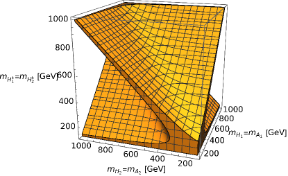
(a) $T$

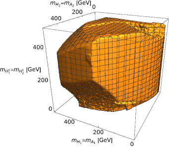
(b) unitarity

Figure 1: Regions allowed by the $T$-parameter at 99% level (a) and unitarity (b) for the $(v,0,0)$ vacuum in the $m_{H_{1}}=m_{A_{1}}$ vs. $m_{H_{2}}=m_{A_{2}}$ vs. $m_{H_{1}^{\pm}}=m_{H_{2}^{\pm}}$ space. The 4th free parameter, the mass of the SM-like Higgs $m_{h}$, is set to 125.25 GeV. On the left panel we additionally assume that all masses are larger than $m_{h}$ while on the right one that they are larger than 1 GeV.

3.2 The $(v,v,v)$ case

In this case the scalar and pseudoscalar Higgses have, separately, common masses: $m_{H_{1}}=m_{H_{2}}$ and $m_{A_{1}}=m_{A_{2}}$. The $T$-parameter allowed region in Fig. 2(a) has the same features as the one in Fig. 1(a), giving analogous relations between masses of $SU(2)_{L}$ doublet components. Unitarity also puts a similar limit on the masses requiring them to be smaller than about 500 GeV (Fig. 2(b)). No points are excluded by HiggsBounds and, similarly as before, HiggsSignals limits masses to $\text{min}(m_{H_{1}},m_{A_{1}})>m_{h}/2$ and $m_{H^{\pm}}\gtrsim 95$ GeV. The same arguments hold as in the case of $(v,0,0)$, including lack of VBF and Higgsstrahlung processes. The lack of VBF and Higgsstrahlung processes for $(v,v,v)$ case follows from the fact, as explained in Sec. 2.4, that the SM-like Higgs does not change between the Higgs basis and mass eigenstates meaning that non-SM Higgses do not possess a VEV – the same as in the $(v,0,0)$ case.

The example point fulfilling unitarity and $T$-parameter constraint ($T=0.03$) is $m_{H}=198.6$ GeV, $m_{A}=202.4$ GeV, $m_{H^{\pm}}=172.3$ GeV.

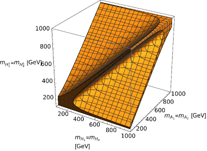
(a) $T$

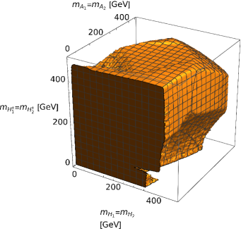
(b) unitarity

Figure 2: Regions allowed by the $T$-parameter at 99% level (a) and unitarity (b) for the $(v,v,v)$ vacuum in the $m_{H_{1}}=m_{H_{2}}$ vs. $m_{A_{1}}=m_{A_{2}}$ vs. $m_{H_{1}^{\pm}}=m_{H_{2}^{\pm}}$ space. The 4th free parameter, the mass of the SM-like Higgs $m_{h}$, is set to 125.25 GeV. On the left panel we additionally assume that all masses are larger than $m_{h}$ while on the right one that they are larger than 1 GeV.

3.3 The $(\omega v,v,v)$ case

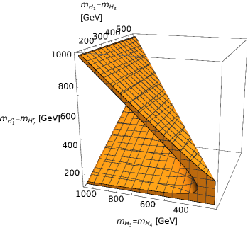
(a) $T$

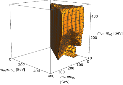
(b) unitarity

Figure 3: Regions allowed by the $T$-parameter at 99% level (a) and unitarity (b) for the $(\omega v,v,v)$ vacuum in the $m_{H_{1}}=m_{H_{2}}$ vs. $m_{H_{3}}=m_{H_{4}}$ vs. $m_{H_{1}^{\pm}}=m_{H_{2}^{\pm}}$ space. The 4th free parameter, the mass of the SM-like Higgs $m_{h}$, is set to 125.25 GeV. On the left panel we additionally assume that all masses are larger than $m_{h}$ while on the right one that they are larger than 1 GeV.

In this case CP is ill-defined so we label all neutral mass eigenstates beyond the SM-like state $h$ as $H_{i}$ ($i=1\ldots 4$). We find pairwise mass degeneracies, with $H_{1}$, $H_{2}$ sharing one mass and $H_{3}$ and $H_{4}$ sharing another one. As explained in Sec. 2.2.4 there is a double degeneracy in solution for potential parameters for a given set of masses. Qualitatively, the allowed region of masses is the same in both cases therefore in Fig. 3 we only plot one of the solutions. Most of the features of Fig. 3 where already present in Figs. 1 and 2 with the distinctive feature in the current case being mainly the condition $m_{H_{3}}>\sqrt{3}m_{H_{1}}$.

An example point passing all phenomenological constraints is: $m_{H_{1}}=m_{H_{2}}=158.6$ GeV, $m_{H_{3}}=m_{H_{4}}=314.3$ GeV, $m_{H^{\pm}}=149.7$ GeV with $T=0.03$, fulfilled unitarity bound and not excluded by HiggsBounds and HiggsSignals.

3.4 Comment on unitarity

As seen from the discussion in this section, the unitarity provides a very strong constraint, limiting all masses to $\lesssim 500$ GeV irrespectively of the chosen vacuum. This is relatively easy to understand. As masses increase, so must the absolute values of couplings as the mass scale is fixed by the EWSB scale. Qualitatively, regions allowed by unitarity are roughly given by $max\{|s|,|r_{1}|,|r_{2}|,|d|\}\lesssim\pi$. We emphasise though that in our analysis we consider also finite energy contributions to the scattering matrix, making it sensitive also to 3-point interactions originating from Eq. (2) after the electroweak symmetry breaking.

4 Conclusions

We have described an extension of the Standard Model with 3 Higgs doublets and the potential invariant under the $\Delta(27)$ symmetry. After covering the known tree-level minima of this potential, we gave formulas for the physical parameters (masses) in terms of the potential parameters and then proceed to constrain the parameter space of the model through $STU$, unitarity as well as certain flavour violation processes. We concluded that unitarity provides a rather strong constraint and keeps the scalar masses below around 500 GeV. We considered assignments of the fermions under the $\Delta(27)$ symmetry that give Yukawa structures leading to distinct masses for each generation and the unit CKM matrix (which we consider a reasonable leading order approximation). Based on that toy model of Yukawa couplings, we were able to test contributions of the additional scalars to flavour violating processes. Using $b\rightarrow s\gamma$ as an example, we concluded that flavour violating processes are tamed by the imposed discrete symmetry. The Higgs mediated neutral flavour changing contributions are suppressed by ratios of the mass of the down-type quark in the loop to the mass of the heavy Higgs. In our model, whenever such contributions are present, two flavour changing neutral vertices are needed implying that the quark in the loop is the down quark, which is extremely light compared to the mass of the heavy Higgs.

Appendix A Group theory of $\Delta(27)$

$\Delta(27)$ is a discrete subgroup of $SU(3)$ with two complex 3-dimensional and 9 distinct 1-dimensional irreducible representations. Here we label one of the 3-dimensional ones as the anti-triplet $\bar{\mathbf{3}}$, the other as the triplet $\mathbf{3}$, and label the singlets as $\mathbf{1}_{k,l}$ ($k,l=0,1,2$) — where the labels $k,l$ denote the transformation properties under the order 3 generators $c$, $d$ of the group ($c^{3}=1$ and $d^{3}=1$). The generators for 1-dimensional representations are simply the phases (powers of $\omega\equiv e^{i\frac{2\pi}{3}}$). In a convenient basis, which we use throughout, for the triplet and anti-triplet representation we have

$$c_{3,\bar{3}}=\begin{pmatrix}0&1&0\\ 0&0&1\\ 1&0&0\end{pmatrix}$$ (125)

$$d_{3}=\begin{pmatrix}1&0&0\\ 0&\omega&0\\ 0&0&\omega^{2}\end{pmatrix}$$ (126)

$$d_{\bar{3}}=\begin{pmatrix}1&0&0\\ 0&\omega^{2}&0\\ 0&0&\omega\end{pmatrix}$$ (127)

With this notation, as the generators of the group are of order 3, the trivial singlet is obtained from products of singlets where the labels add up to zero modulo 3. The product of a triplet and anti-triplet results in all nine singlets whereas the product of two anti-triplets yields three triplets and vice-versa as follows

$$\mathbf{3}\otimes\mathbf{3} = \bar{\mathbf{3}}_{S_{1}}\oplus\bar{\mathbf{3}}_{S_{2}}\oplus\bar{\mathbf{3}}_{A}$$

$$\bar{\mathbf{3}}\otimes\bar{\mathbf{3}} = \mathbf{3}_{S_{1}}\oplus\mathbf{3}_{S_{2}}\oplus\mathbf{3}_{A}$$

$$\mathbf{3}\otimes\bar{\mathbf{3}} = \sum_{r=0}^{2}\mathbf{1}_{r,0}\oplus\sum_{r=0}^{2}\mathbf{1}_{r,1}\oplus\sum_{r=0}^{2}\mathbf{1}_{r,2}$$

$$\mathbf{1}_{k,\ell}\otimes\mathbf{1}_{k^{\prime},\ell^{\prime}} = \mathbf{1}_{k+k^{\prime}~{}mod~{}3,\ell+\ell^{\prime}~{}mod~{}3}$$ (128)

The specific composition rules for the (anti-)triplet products are

$$\left(\mathbf{3}\otimes\mathbf{3}\right)_{\bar{\mathbf{3}}_{S_{1}}} = \left(x_{1}y_{1},x_{2}y_{2},x_{3}y_{3}\right),$$

$$\left(\mathbf{3}\otimes\mathbf{3}\right)_{\bar{\mathbf{3}}_{S_{2}}} = \frac{1}{2}\left(x_{2}y_{3}+x_{3}y_{2},x_{3}y_{1}+x_{1}y_{3},x_{1}y_{2}+x_{2}y_{1}\right),$$

$$\left(\mathbf{3}\otimes\mathbf{3}\right)_{\bar{\mathbf{3}}_{A}} = \frac{1}{2}\left(x_{2}y_{3}-x_{3}y_{2},x_{3}y_{1}-x_{1}y_{3},x_{1}y_{2}-x_{2}y_{1}\right),$$

$$\left(\mathbf{3}\otimes\bar{\mathbf{3}}\right)_{\mathbf{1}_{r,0}} = x_{1}y_{1}+\omega^{2r}x_{2}y_{2}+\omega^{r}x_{3}y_{3},$$

$$\left(\mathbf{3}\otimes\bar{\mathbf{3}}\right)_{\mathbf{1}_{r,1}} = x_{1}y_{2}+\omega^{2r}x_{2}y_{3}+\omega^{r}x_{3}y_{1},$$

$$\left(\mathbf{3}\otimes\bar{\mathbf{3}}\right)_{\mathbf{1}_{r,2}} = x_{1}y_{3}+\omega^{2r}x_{2}y_{1}+\omega^{r}x_{3}y_{2},$$ (129)

where $r=0,1,2$, and $\left(x_{1},x_{2},x_{3}\right)$ and $\left(y_{1},y_{2},y_{3}\right)$ are the components of the (anti-)triplets in the product. Care should be taken in the product of a triplet and anti-triplet as the ordering is relevant. The subscript for the product of a triplet and an anti-triplet resulting in a singlet specifies which of the singlets it transforms as, whereas the product of two triplets (or two anti-triplets) results in distinct anti-triplets (or triplets), where the subscripts denote if it is a symmetric product ($S_{1}$, $S_{2}$) or an anti-symmetric one ($A$).

Appendix B SPheno setup

For numerical analysis we use SPheno in the OnlyLowEnergySPheno setup. Higgs boson masses are computed purely at the tree level and parameter points are specified in terms of physical Higgs masses, with scalar potential parameters extracted using Eqs. (12)–(15), (20)–(23) or (33)–(36). We equate 3HDM VEVs (with obvious numerical prefactors) to the SM VEV fixed to $v_{\text{SM}}\equiv\left(\sqrt{2}G_{F}\right)^{-1/2}$, with $G_{F}=1.1663787\cdot 10^{-5}$ GeV^-2. No RGE running is performed, so through calculation of all observables (unitarity, $STU$, etc.) the same values of $s$, $r_{1}$, $r_{2}$ and $d$ are used. There is however a small difference in gauge and Yukawa couplings used in different parts of the code due to how SPheno extracts them from SM input parameters.

We use the following settings in SPheno to check the unitarity constraints

⬇

1BLOCK SPhenoInput

2 440 1 # Tree-level unitarity constraints (limit s->infinity)

3 441 1 # Full tree-level unitarity constraints

4 442 1. # sqrt(s_min)

5 443 5000. # sqrt(s_max)

6 444 -1000 # steps

7 445 0 # running

8 445 2 # Cut-Level for T/U poles

Technically, as for the (finite) maximal energy of 5 TeV, occasionally the maximal scattering eigenvalue $\lambda_{\text{max}}^{\text{finite}~{}S}<\lambda_{\text{max}}^{S\to\inf}$ we plot the region where $max(\lambda_{\text{max}}^{\text{finite}~{}S},\lambda_{\text{max}}^{S\to\inf})<\tfrac{1}{2}$. Here $\lambda_{\text{max}}^{\text{finite}~{}S}$ $(\lambda_{\text{max}}^{S\to\inf})$ is the eigenvalue as given in block TREELEVELUNITARITYwTRILINEARS (TREELEVELUNITARITY) of SPheno’s SLHA Skands:2003cj ; Allanach:2008qq ; Goodsell:2018tti output.

Appendix C Example decay patterns of non-SM Higgs bosons

Example of decay patters of non-SM Higgses for the $(v,0,0)$ vacuum and $m_{H_{1}}=200$ GeV, $m_{H_{2}}=300$ GeV and $m_{H_{2}^{\pm}}=400$ GeV as given by the created 3HDM SPheno spectrum generator. In the extract of the SLHA output below, H0_2, A0_2, Hp_2 correspond to $H_{2}$, $A_{1}$ and $H^{\pm}_{1}$, respectively. For other particles standard SPheno symbols and indexing are used.

⬇

DECAY 45 7.97690384E+00 # H0_2

# BR NDA ID1 ID2

1.29114182E-02 2 36 23 # BR(H0_2 -> A0_2 VZ )

3.23331057E-04 2 -1 5 # BR(H0_2 -> Fd_1^* Fd_3 )

3.23497669E-04 2 -3 5 # BR(H0_2 -> Fd_2^* Fd_3 )

3.23331057E-04 2 -5 1 # BR(H0_2 -> Fd_3^* Fd_1 )

3.23497669E-04 2 -5 3 # BR(H0_2 -> Fd_3^* Fd_2 )

2.46405648E-01 2 -2 6 # BR(H0_2 -> Fu_1^* Fu_3 )

2.46424262E-01 2 -4 6 # BR(H0_2 -> Fu_2^* Fu_3 )

2.46405648E-01 2 -6 2 # BR(H0_2 -> Fu_3^* Fu_1 )

2.46424262E-01 2 -6 4 # BR(H0_2 -> Fu_3^* Fu_2 )

DECAY 36 7.60203352E-01 # A0_2

# BR NDA ID1 ID2

9.65338080E-04 2 -1 5 # BR(A0_2 -> Fd_1^* Fd_3 )

9.65695420E-04 2 -3 5 # BR(A0_2 -> Fd_2^* Fd_3 )

9.65338080E-04 2 -5 1 # BR(A0_2 -> Fd_3^* Fd_1 )

9.65695420E-04 2 -5 3 # BR(A0_2 -> Fd_3^* Fd_2 )

1.36165292E-04 2 -11 15 # BR(A0_2 -> Fe_1^* Fe_3 )

1.36636215E-04 2 -13 15 # BR(A0_2 -> Fe_2^* Fe_3 )

1.36165292E-04 2 -15 11 # BR(A0_2 -> Fe_3^* Fe_1 )

1.36636215E-04 2 -15 13 # BR(A0_2 -> Fe_3^* Fe_2 )

2.49066556E-01 2 -2 6 # BR(A0_2 -> Fu_1^* Fu_3 )

2.48685848E-01 2 -4 6 # BR(A0_2 -> Fu_2^* Fu_3 )

2.49066556E-01 2 -6 2 # BR(A0_2 -> Fu_3^* Fu_1 )

2.48685848E-01 2 -6 4 # BR(A0_2 -> Fu_3^* Fu_2 )

DECAY 37 3.06760690E+01 # Hp_2

# BR NDA ID1 ID2

1.11313431E-01 2 36 24 # BR(Hp_2 -> A0_2 VWp )

6.11469833E-03 2 46 24 # BR(Hp_2 -> A0_3 VWp )

2.96841032E-04 2 -1 6 # BR(Hp_2 -> Fd_1^* Fu_3 )

7.64780553E-01 2 -5 4 # BR(Hp_2 -> Fd_3^* Fu_2 )

1.11313431E-01 2 35 24 # BR(Hp_2 -> H0_1 VWp )

6.11469833E-03 2 45 24 # BR(Hp_2 -> H0_2 VWp )

The entirety of the above output is attached to the arXiv version of this work.