Spectrum of kinetic plasma turbulence at 0.3$-$0.9 astronomical units from the Sun

Abstract

We investigate spectral properties of turbulence in the solar wind that is a weakly collisional astrophysical plasma, accessible to in-situ observations. Using the Helios search coil magnetometer measurements in the fast solar wind, in the inner heliosphere, we focus on properties of the turbulent magnetic fluctuations at scales smaller than the ion characteristic scales, the so-called kinetic plasma turbulence. At such small scales, we show that the magnetic power spectra between 0.3 and 0.9 AU from the Sun have a generic shape $\sim f^{-8/3}\exp{(-f/f_{d})}$ where the dissipation frequency $f_{d}$ is correlated with the Doppler shifted frequency $f_{\rho e}$ of the electron Larmor radius. This behavior is statistically significant: all the observed kinetic spectra are well described by this model, with $f_{d}=f_{\rho e}/1.8$. Our results indicate that the electron gyroradius plays the role of the dissipation scale and marks the end of the electromagnetic cascade in the solar wind.

I Introduction

Astrophysical plasmas are often very rarefied so that the Coulomb collisions are infrequent [e.g., Meyer-Vernet, 2007, Salem et al., 2003]: in contrast to the usual neutral fluids, the collisional dissipation (viscous and resistive) channels are weak, and the Kolomogorov’s dissipation scale Frisch [1995] is ill-defined. Furthermore, the presence of a background magnetic field $\bm{B_{0}}$ introduces a preferred direction [e.g., Shebalin et al., 1983, Oughton et al., 1994, Verdini et al., 2015, Oughton and Matthaeus, 2020] and allows the existence of propagating incompressible modes (Alfvén waves). The different plasma ion and electron constituents have a number of characteristic (kinetic) scales at which properties of turbulent fluctuations change.

Considering all this complexity, one may wonder whether there is a certain degree of generality in space plasma turbulence. In particular, does the dissipation range have a general spectrum, as is the case in neutral fluid turbulence Chen et al. [1993], Frisch [1995]?

The solar wind plasma, which is accessible to in-situ space exploration, has proven to be a very useful laboratory to study the astrophysical plasma turbulence [e.g., Bruno and Carbone, 2013, Alexandrova et al., 2013]. Since the first early in-situ measurements, [e.g., Coleman, 1968], our knowledge of the large-scale turbulence in the solar wind has greatly improved, [e.g., Bruno and Carbone, 2013, Kiyani et al., 2015]. There is an extended inertial range of scales at which incompressible magnetohydrodynamics (MHD) phenomenologies Goldreich and Sridhar [1995], Boldyrev [2005], Chandran et al. [2015], similar in spirit to Kolomogorov’s phenomenology, may be invoked to understand the formation of a Kolmogorov-like spectrum of magnetic fluctuations $\sim k^{-5/3}$. (Note that satellite measurements are time series, thus, in Fourier space one gets frequency spectra. At the radial distances from the Sun studied here, any characteristic plasma velocity, except whistler wave phase speed, is less than the solar wind speed $V$. Thus, one can invoke Taylor’s hypothesis and convert a spacecraft-frame frequency $f$ to a flow-parallel wavenumber $k$ in the plasma frame $k=2\pi f/V$.)

At the short wavelength end of the inertial domain, i.e., at scales of the order of the proton inertial scale $\lambda_{p}=c/\omega_{pp}$ (where $c$ is the speed of light and $\omega_{pp}$ is the proton plasma frequency) the spectrum steepens. At these scales ($\sim 100$ km at 1 AU from the Sun ), the MHD approximation is no longer valid; the “heavy” ion (basically, a proton in the solar wind) fluid and the “light” electron fluid behave separately, [e.g., Matthaeus et al., 2008, Hellinger et al., 2018, Papini et al., 2019]. It is still not completely clear whether the spectral steepening at ion scales is the beginning of the dissipation range or a transition to another cascade taking place between ion and electron scales or a combination of both [e.g., Alexandrova et al., 2013, Chen, 2016, Li et al., 2019]. Recent von Kármán-Howarth analyses of direct numerical simulations and in-situ observations Hellinger et al. [2018], Bandyopadhyay et al. [2020] indicated that the transition from the MHD inertial range to the sub-ion range is due to a combination of the onset of the Hall MHD effect and a reduction of the cascade rate likely due to some dissipation mechanism. Then, the question arises as to how much of the dissipation of the turbulent energy is flowing into the ions and how much is flowing into the electrons. In the vicinity of the electron scales ($\sim 1$ km at 1 AU), the fluid description no longer holds, and the electrons should be considered as particles. The present paper focuses on this short wavelength range, i.e., between the ion scales and a fraction of the electron scales.

The first solar wind observations of turbulence at scales smaller than ion scales (the so-called sub-ion scales) were reported by Denskat et al. [1983], using the search coil magnetometer (SCM) on Helios space mission at radial distances $R\in[0.3,0.9]$ AU from the Sun. From this pioneering work we know that between the ion and electron scales, the magnetic spectrum follows an $\sim f^{-3}$ power law.

Thanks to the Spatio-Temporal Analysis of Field Fluctuations (STAFF) instrument on Cluster space mission [Escoubet et al., 1997, Cornilleau-Wehrlin et al., 1997], which is the most sensitive SCM flown in the solar wind to date, the small scale tail of the electromagnetic cascade at 1 AU could be explored down to a fraction of electron scales $\sim 0.2-1$ km [Mangeney et al., 2006, Alexandrova et al., 2008, 2009, 2012, 2013, Sahraoui et al., 2010, 2013, Lacombe et al., 2017, Matteini et al., 2017], i.e., up to 1/5 of electron scales. These observations seem confusing at first glance: the spectral shape of the magnetic fluctuations varies from one record to another, suggesting that the spectrum is not universal at kinetic scales [Mangeney et al., 2006, Sahraoui et al., 2010, 2013]. However, as was shown in [Lacombe et al., 2014, Roberts et al., 2017, Matteini et al., 2017], most of these spectral variations are due to the presence, or absence, of quasi-linear whistler waves with frequencies at a fraction of the electron cyclotron frequency $f_{ce}=eB_{0}/(2\pi m_{e})$ (where $e$ and $m_{e}$ are the charge and the mass of an electron, respectively) and wave vectors $\bm{k}$ quasi-parallel to $\bm{B_{0}}$ [Lacombe et al., 2014]. These waves may result from the development of some instabilities associated with either an increase of the electron temperature anisotropy or an increase of the electron heat flux in some regions of the solar wind Štverák et al. [2008]. In the absence of whistlers, the background turbulence is characterized by low frequencies in the plasma frame and wave vectors mostly perpendicular to the mean field $\bm{k}\perp\bm{B_{0}}$ [Lacombe et al., 2017]. This quasi-2D turbulence is convected by the solar wind (with the speed $\bm{V}$) across the spacecraft and appears in the satellite frame at frequencies $f=k_{\perp}V/2\pi$. It happens that these frequencies are below but close to $f_{ce}$, exactly in the range where whistler waves (with $\bm{k}\;\|\;\bm{B_{0}}$ and $f\simeq(0.1-0.2)f_{ce}$) may appear locally. Therefore, the superposition of turbulence and whistlers at the same frequencies is coincidental. If we could perform measurements directly in the plasma frame, these two phenomena would be completely separated in $\bm{k}$ and $f$. A possible interaction between turbulence and whistlers is out of the scope of the present paper. We focus here on the background turbulence at kinetic scales only.

A statistical study by Alexandrova et al. [2012] of solar wind streams at 1 AU under different plasma conditions showed that, in the absence of parallel whistler waves, the quasi-2D background turbulence forms a spectrum $\sim k_{\perp}^{-8/3}\exp{(-k_{\perp}\ell_{d})}$, with a cut-off scale $\ell_{d}$ well correlated with the electron Larmor radius $\rho_{e}=\sqrt{2k_{B}T_{e\perp}/m_{e}}/(2\pi f_{ce})$ (where $k_{B}$ is the Boltzmann constant and $T_{e\perp}$ is the electron perpendicular temperature). Such a spectrum with an exponential correction indicates a lack of spectral self-similarity at electron scales, as in the dissipation range of the neutral flow turbulence. How general is this kinetic spectrum? Is it observed closer to the Sun than 1 AU?

Parker Solar Probe (PSP) observations in the slow wind at $0.17$ AU show a spectrum close to $\sim f^{-8/3}$ at sub-ion scales Bale and et al. [2019]. In a statistical study of turbulent spectra up to 100 Hz, Bowen et al. [2020] determined spectral indices up to 30 Hz, confirming a power law usually observed at 1 AU $\sim f^{-2.8}$ Alexandrova et al. [2009], Chen et al. [2010], Alexandrova et al. [2012], Kiyani et al. [2013], Sahraoui et al. [2013]. The PSP–SCM data products up to 100 Hz used in [Bale and et al., 2019, Bowen et al., 2020] and the instrumental noise level do not allow the resolution of electron scales at $0.17$ AU, at least for the types of solar wind and the Sun-spacecraft distances sampled by PSP to date.

In this paper, we analyze magnetic spectra within the $[7,700]$ Hz range at radial distances between 0.3 and 0.9 AU thanks to Helios measurements. Here, for the first time, we provide a turbulent spectrum at electron scales and its simple empirical description at distances from the Sun smaller than 1 AU. The spectrum follows a function similar to that found at 1 AU, indicating generality of the phenomenon.

II Data

The SCM instrument on Helios space mission Neubauer et al. [1977a] consists of three orthogonally oriented search coil sensors which are mounted on a boom at a distance of 4.6 m from the center of the spacecraft with the $z$-sensor parallel to the spin axis and $x$ and $y$ sensors in the spin plane. The wave forms from the sensors are processed in an on-board spectrum analyzer. They pass through 8 band-pass filters which are continuous in frequency coverage and logarithmically spaced. The central frequencies of the 8 channels are 6.8, 14.7, 31.6, 68, 147, 316, 681 and 1470 Hz. The novel feature for the time of construction of the instrument was that the filter outputs were processed by a digital mean-value-computer on board of Helios Neubauer et al. [1977b].

Thus, the instrument provides magnetic spectra for two of three components, $(B_{y},B_{z})$ and rarely $(B_{x},B_{z})$, in the Spacecraft Solar Ecliptic reference frame, which is equivalent to the Geocentric Solar Ecliptic frame . The available Helios-SCM products are the spectra integrated over 8 s. For the present study we use only the spectra of $B_{y}$. Indeed, the pre-flight noise level for the $B_{y}$ spectra matches well the post-flight noise level, which is not the case for $B_{z}$. More details on the instrument and data processing can be found in [Neubauer et al., 1977b].

We have analyzed 246543 individual $B_{y}$–magnetic spectra as measured by SCM on Helios–1 with signal-to-noise ratios (SNR) larger than or equal to 2 up to 100 Hz, at radial distances from the Sun $R\in[0.3,0.9]$ AU Among them, about $2\%$ of the spectra show spectral bumps between the lower hybrid frequency $f_{lh}$ and $\sim 0.25f_{ce}$ Jagarlamudi et al. [2020]. Such bumps are the signatures of parallel whistler waves as was shown in Lacombe et al. [2014]. The analysis of these spectra with bumps, shows that the signatures of whistlers are mostly present in the slow wind ($V<500$ km/s) and their appearance increases with the distance from the Sun Jagarlamudi et al. [2020]. In the fast wind ($V>600$ km/s) and close to the Sun, we do not observe signatures of whistlers in 8-s individual spectra of Helios–SCM. Here, we analyze background turbulence spectra in the fast solar wind, i.e., without signatures of whistler waves.

On the basis of this first analysis of 246543 $B_{y}$–spectra with a SNR $\geq 2$ up to 100 Hz, we can already say that the background turbulence without signatures of whistlers is commonly observed (98% of the analyzed spectra) and its spectral shape is very similar at different radial distances as we will see below, just the amplitude changes. Turbulent level decreases with radial distance Beinroth and Neubauer [1981], Denskat et al. [1983], Bourouaine et al. [2012], Chen et al. [2020] and thus further from the Sun, fewer SCM frequencies are resolved. For the statistical study, we will consider 3344 spectra with a SNR larger than or equal to 3 up to $316$ Hz and among them 39 spectra with a SNR $\geq 3$ up to $681$ Hz. All these 3344 spectra are at 0.3 AU.

III Spectral analysis

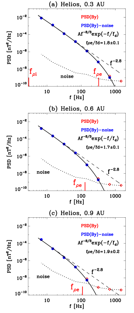
Figure 1: Examples of the most intense Helios–SCM spectra of $B_{y}$ component, as functions of the spacecraft-frame frequency $f$, at (a) 0.3 AU, (b) 0.6 AU and (c) 0.9 AU. For the 3 radial distances, the raw-spectrum is shown by red diamonds, the corrected spectrum, after the subtraction of the noise – by blue dots, the black solid line gives the fit with the model function (1), the dashed line gives $f^{-2.8}$ power-law for comparison and the dotted line indicates the noise level of the Helios-SCM-$B_{y}$. Vertical red lines give the Doppler shifted kinetic scales: in (a), $\rho_{p}$ and $\rho_{e}$ appear at $f_{\rho p}=2.9$ Hz and $f_{\rho e}=325$ Hz, respectively; in (b) they appear at $f_{\rho p}\simeq 1$ Hz and $f_{\rho_{e}}=130$ Hz, respectively; and in (c) they appear at $f_{\rho p}\simeq 1$ Hz and $f_{\rho_{e}}=110$ Hz, respectively.

Figure 1(a)-(c) show examples of the most intense $B_{y}$–spectra as measured by SCM on Helios–1 at 0.3, 0.6 and 0.9 AU, respectively. For the 3 radial distances from the Sun the raw power spectral densities (PSDs) are shown by red diamonds. The dotted line indicates the noise level of the instrument for the $B_{y}$–component. The spectra corrected for the noise contribution by the subtraction of the noise level are shown by blue dots. Vertical red lines give the Doppler shifted kinetic scales. Plasma parameters, characteristic lengths and frequencies corresponding to these spectra are given in Table 1.

We perform a least square fit of the 3 corrected spectra with the model function known to describe the kinetic spectrum at 1 AU Alexandrova et al. [2012]:

$$P_{\text{model}}(f)=Af^{-8/3}\exp{(-f/f_{d})}.$$ (1)

This model has two free parameters: the amplitude of the spectrum $A$ and the dissipation frequency $f_{d}$. The result of this fitting is shown by a black solid line in the 3 cases. The corresponding maximal physical frequencies $f_{max}$ (the highest frequency where the SNR is $\geq 3$ still verifies Alexandrova et al. [2010]) together with the results of the fit are given at the end of Table 1. At 0.3 AU, the spectrum is well resolved up to $f_{max}=681$ Hz (the 7th out of the 8 SCM frequencies). The electron Larmor radius $\rho_{e}\simeq 0.4$ km appears at $f_{\rho e}=V/(2\pi\rho_{e})=325$ Hz (see the right vertical red line). Thus, in this case, turbulence is resolved up to a minimal scale of about $\ell_{min}=V/(2\pi f_{max})=0.47\rho_{e}$ (see the bottom row of Table 1). As expected Beinroth and Neubauer [1981], Denskat et al. [1983], Bourouaine et al. [2012], Chen et al. [2020], further from the Sun the intensity of the spectra decreases with $R$: at 0.6 AU, the spectrum is resolved up to 316 Hz and at 0.9 AU, it is resolved only up to 147 Hz. In both cases, nonetheless, the electron Larmor radius is resolved as $\rho_{e}\sim 1/B_{0}$ increases with $R$ and the corresponding frequency $f_{\rho e}$ decreases (see vertical red lines in Figure 1(b) and (c): $f_{\rho e}=130$ Hz at 0.6 AU and $110$ Hz at 0.9 AU). The observed spectra at 3 radial distances from the Sun are well described by the model, and the dissipation frequency $f_{d}$ decreases from $(183\pm 5)$ Hz at 0.3 AU to $(56\pm 4)$ Hz at $0.9$ AU, following $f_{\rho e}$.

From Table 1 one can see that further from the Sun, the relative errors on free parameters of the fit, $\Delta f_{d}/f_{d}$ and $\Delta A/A$, increase, while the $f_{max}$ decreases. This error increase is expectable: $f_{max}$ is proportional to the turbulence level, and the lower turbulence level corresponds to the smaller SNR and automatically to a smaller number of frequencies to fit; thus, we get higher errors.

Table 1: Plasma parameters, characteristic scales and frequencies, maximal resolved frequency by Helios/SCM, $f_{max}$, and results of the fit to Eq.(1) at 3 radial distances from the Sun, corresponding to the spectra in Figure 1. The two bottom rows indicate a fraction of $\ell_{d}$ and $\rho_{e}$–scales resolved by these spectra.

$R$ (AU)	0.9	0.6	0.3
$B_{0}$ (nT)	$8.5$	11.6	$32.2$
$V$ (km/s)	$720$	710	$740$
$n_{p}$ (cm-3)	$4.8$	7.0	$28.4$
$T_{p}$ (eV)	$34.3$	51.1	$61.2$
$T_{e}$ (eV)	$9.3$	12.7	$12.9$
$T_{p\perp}$ (eV)	$41.2$	67.8	$80.3$
$T_{e\perp}$ (eV)	$7.0$	9.0	$12$
$\beta_{p,\perp}$	$1.1$	1.4	$0.9$
$\beta_{e,\perp}$	$0.2$	0.2	$0.13$
$\lambda_{p}$ (km)	$99$	82	$41$
$\rho_{p}$ (km)	$109$	102	$40$
$\lambda_{e}$ (km)	$2.3$	1.9	$1$
$\rho_{e}$ (km)	$1.0$	0.9	$0.4$
$f_{cp}$ (Hz)	$0.10$	0.2	$0.5$
$f_{\lambda p}$ (Hz)	$1.2$	1.4	$2.9$
$f_{\rho p}$ (Hz)	$1.0$	1.1	$2.9$
$f_{\lambda e}$ (Hz)	$50$	59	$124$
$f_{\rho e}$ (Hz)	$110$	130	$325$
$f_{ce}$ (Hz)	$238$	325	$900$
$f_{max}$ (Hz)	147	316	681
$A$ (nT${}^{2}/$Hz)Hz8/3	$0.04$	$0.34$	$1.63$
$\Delta A/A$	2	0.2	0.03
$f_{d}$ (Hz)	$56$	$58$	$183$
$\Delta f_{d}/f_{d}$	0.07	0.04	0.03
$f_{d}/f_{max}$	0.38	0.27	0.27
$f_{\rho e}/f_{max}$	0.74	0.40	0.47

Now let us consider the most intense spectra, i.e., with a SNR that is $\geq 3$ up to $681$ Hz and with simultaneous measurements of $\bm{B_{0}}$. These conditions are verified for 39 spectra at 0.3 AU in the fast wind, measured during the closest approach of Helios to the Sun.

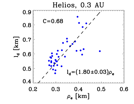
Figure 2: Results of the fitting procedure of the most intense spectra at 0.3 AU with Eq. (1): dissipation scale $\ell_{d}=V/2\pi f_{d}$ as a function of the electron Larmor radius $\rho_{e}$; the linear dependence $\ell_{d}=1.8\rho_{e}$ is indicated by the dashed line, with the correlation coefficient $C=0.68$.

All these spectra are similar to that shown in Figure 1(a). We perform a least squares fit of the 39 spectra with the model function, Eq. (1). The relative errors, $\Delta f_{d}/f_{d}$ and $\Delta A/A$, vary between 0.01 and 0.14. The dissipation scale $\ell_{d}$ can be estimated using the Taylor hypothesis $\ell_{d}=V/(2\pi f_{d})$. It is found to be correlated with the $\rho_{e}$ scale with a correlation coefficient $C=0.68$. The relation $\ell_{d}\sim 1.8\rho_{e}$ is observed (see Figure 2). There is no correlation with the electron inertial length $\lambda_{e}$ ($C=0.02$, not shown). Thus, we can fix $f_{d}$ in Eq. (1):

$$P_{\text{model}}(f)=Af^{-8/3}\exp{(-1.8f/f_{\rho e})}.$$ (2)

Let us now verify whether this simpler model describes a larger statistical sample.

To increase the number of spectra analysed, we now also consider less resolved spectra, i.e., with a signal-to-noise ratio larger than 3 up to 316 Hz, and with plasma measurements in the vicinity of the spectra (i.e., the mean field at most within 16 s around the measured SCM spectrum, the electron temperature $T_{e}$ within about 30 min; and when not available, $T_{e}$ is taken within a longer time interval but within the same wind type). These conditions are verified for 3344 spectra at 0.3 AU in the fast wind. Probability distribution functions (PDFs) of the mean plasma parameters for the 3344 spectra are shown in Figure 3 with black lines and those for the 39 most intense spectra analyzed above, are shown by green lines. The proton $\beta_{p}$ (electron $\beta_{e}$) plasma beta is the ratio between the proton (electron) thermal pressure and the magnetic pressure. From these PDFs, we see that the 39 most intense spectra are observed for the solar wind with $V>650$ km/s, for the proton thermal pressure $n_{p}k_{B}T_{p}\geq 0.2$ nPa and for the largest $\beta_{p}$ and $\beta_{e}$ values of the analyzed data set (for $\beta_{p}\geq 0.3$ and $\beta_{e}\geq 0.1$).

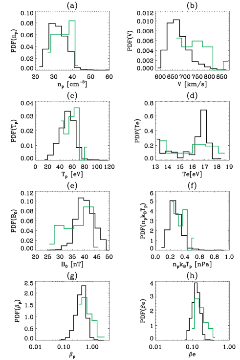
Figure 3: Probability distribution functions (PDF’s) of the mean plasma parameters at 0.3 AU for the 3344 spectra shown in Figure 4 (black lines) and for the 39 most intense spectra (green lines): (a) proton density $n_{p}$, (b) solar wind speed $V$, (c) proton temperature $T_{p}$, (d) electron temperature $T_{e}$, (e) magnetic field magnitude $B_{0}$, (f) proton thermal pressure $n_{p}k_{B}T_{p}$, (g) proton plasma beta $\beta_{p}$, (h) electron beta $\beta_{e}$.

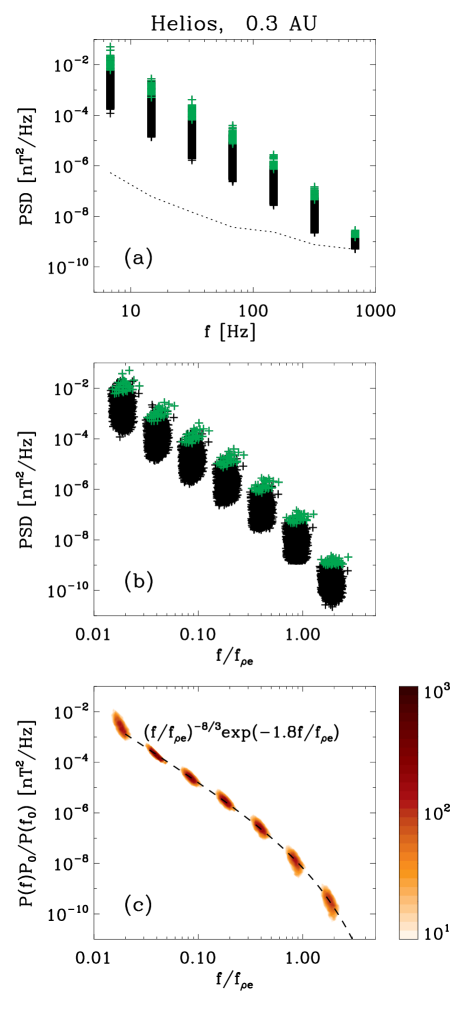
Figure 4: (a) 3344 individual Helios–1 SCM spectra of $B_{y}$ as functions of the spacecraft-frame frequency $f$ at 0.3 AU in the fast wind; the 39 most intense spectra are marked by green crosses; the SCM noise for $B_{y}$ component is indicated by a dotted line. (b) These 3344 spectra corrected for the noise contribution as functions of $f$ normalised to the Doppler shifted electron Larmor radius frequency $f_{\rho e}=V/(2\pi\rho_{e})$. (c) The same spectra, rescaled by their amplitude at $f_{0}=0.051f/f_{\rho e}$ (see the text); the result is shown as a 2D histogram with the number of the data points proportional to the darkness of the red colour. The dashed line displays the model function, Eq.(3).

Figure 4(a) displays the 3344 raw $B_{y}$ spectra, $P_{\text{raw}}(f)$, by crosses. The 39 most intense spectra are marked by green crosses; the noise level for $B_{y}$, $P_{\text{noise}}(f)$ is indicated by the dotted line. Figure 4(b) shows these 3344 spectra corrected for the noise contribution, $P(f)=P_{\text{raw}}(f)-P_{\text{noise}}(f)$, and as functions of $f$ normalised to the Doppler shifted electron Larmor radius frequency, $f_{\rho e}=V/(2\pi\rho_{e})$. Let us now superpose all spectra together. Figure 4(c) shows a 2D histogram calculated with the spectra of the middle panel and rescaled by their amplitude at $f/f_{\rho e}=0.051$, i.e., $P(f)P_{0}/P(f_{0})$. This means that by construction all spectra pass through the point $(f_{0},P_{0})=(0.051f_{\rho e},10^{-4}\mathrm{nT}^{2}/\mathrm{Hz})$; the spectrum amplitudes at $f_{0}$ are linearly interpolated from the two nearest points. The results do not change if we choose another way to adjust the amplitudes in order to bring the spectra together. This rescaling allows us to fix the last free parameter in Eq. (2), the amplitude to a value $A_{0}$, which is now related to $P_{0}$ at $f_{0}$. Thus, we can compare the shape of 3344 spectra with the function

$$P_{\text{model}}(f/f_{\rho e})=A_{0}(f/f_{\rho e})^{-8/3}\exp{(-1.8f/f_{\rho e})}.$$ (3)

This model passes through the data without any fitting; only the frequency is normalized to $f_{\rho e}$, and the amplitude is rescaled at the point $(f_{0},P_{0})$, see the dashed line in Figure 4(c). Note that the dispersion of the data points at the lowest and highest frequency ends can be due to the non simultaneous $T_{e}$ measurements. Moreover, the lowest frequency can be affected as well by the proximity of the ion characteristic scales, and the highest frequencies can be affected by the SCM noise.

IV Conclusion and discussion

These results together with the previous observations at 1 AU [Alexandrova et al., 2012], indicate that at kinetic scales smaller than the ion characteristic scales, the spectrum in the fast wind keeps its shape $\sim f^{-8/3}\exp{(-f/f_{d})}$ independently of the radial distance from the Sun, from 0.3 to 1 AU, with an exponential falloff, reminiscent of the dissipation range of the neutral fluid turbulence. The equivalent of the Kolmogorov scale $\ell_{d}$, where the dissipation of the electromagnetic cascade is expected to take place, is controlled by the electron Larmor radius $\rho_{e}$ for these radial distances. Precisely, here, with Helios we find $\ell_{d}\simeq 1.8\rho_{e}$, and previously, with Cluster at 1 AU, we observed $\ell_{d}\simeq 1.4\rho_{e}$ [Alexandrova et al., 2012]. The constant in front of $\rho_{e}$ seems to be weakly dependent on $R$. This will be verified in a future study with PSP and Solar Orbiter.

The equivalence between $\ell_{d}$ and $\rho_{e}$ is not a trivial result. First, the electron Larmor radius is not the only characteristic length at such small scales. Closer to the Sun, the electron inertial length $\lambda_{e}$ becomes larger than the Larmor radius $\rho_{e}$, but as observed here, it is still with $\rho_{e}$ and not with $\lambda_{e}$ that the “dissipation” scale correlates. Second, in neutral fluids, the dissipation scale $\ell_{d}$ is much larger than the mean free path, so that the dissipation range is described within the fluid approximation. In the solar wind between 0.3 and 1 AU, as we showed, $\ell_{d}$ is defined by $\rho_{e}$ scale. In the vicinity of $\rho_{e}$ the protons are completely kinetic, and electrons start to be kinetic. Third, it appears puzzling that the dissipation scale in space plasma is fixed to a given plasma scale. It is well known in neutral fluids that the dissipation scale $\ell_{d}$ depends on the energy injection rate $\varepsilon$ and thus on the amplitude of turbulent spectrum in the following way: $A\sim\varepsilon^{2}/3\sim\ell_{d}^{-8/3}$ [e.g., Frisch, 1995, Alexandrova et al., 2009]. Is $\rho_{e}$ independent of the energy injection? We found previously that the turbulent spectrum amplitude is anticorrelated with $\rho_{e}$ Alexandrova et al. [2009]; that is, it seems that the electron Larmor radius is sensitive to the turbulence level and thus to the energy injection. We expect to verify this point with PSP and Solar Orbiter data in future studies.

The results presented here may suggest that around the $\rho_{e}$ scale the electron Landau damping is at work to dissipate magnetic fluctuations into electron heating: this is found in 3D gyrokinetic simulations [TenBarge et al., 2013] and in analytical models of strong kinetic Alfvén wave (KAW) turbulence [Passot and Sulem, 2015, Schreiner and Saur, 2017] and can be explained by the weakened cascade model of Howes et al. [2011]. However, in these theoretical and numerical works, the particle distributions are assumed to be Maxwellian, which is not the case in solar wind.

It seems that the electron Landau damping is not the only possible dissipation mechanism. Parashar et al. [2018] observed that the spectral curvature at electron scales is sensitive to the $\rho_{e}$ scale (i.e., to $\beta_{e}$) in 2D Particle-in-cell simulations, where the direction parallel to $\bm{B}_{0}$ is not resolved, so that the Landau damping cannot be effective. Rudakov et al. [2011] studied the weak KAW turbulence and showed that a non-Maxwellian electron distribution function has a significant effect on the cascade: the linear Landau damping leads to the formation of a plateau in the parallel electron distribution function $f(V_{e\|})$, for $V_{A}<V_{e\|}<V_{e,th}$, which reduces the Landau damping rate significantly. These authors studied the nonlinear scattering of waves by plasma particles and concluded that, for the solar wind parameters, this scattering is the dominant process at kinetic scales, with the dissipation starting at the $\lambda_{e}$ scale. To date, we have not measured in the solar wind a plateau in $f(V_{e\|})$ between the Alfvén speed $V_{A}$ and the electron thermal speed $V_{e,th}$. Such a distribution may exist, but would be very difficult to observe because of instrumental effects such as the spacecraft potential and photoelectrons. However, it is not clear to what extent the quasi-linear results based on the Landau damping or the weakly non-linear model of Rudakov et al. [2011] are relevant when non-linear coherent structures [Greco et al., 2016, Perri et al., 2012] importantly contribute to the turbulent power spectrum on kinetic scales.

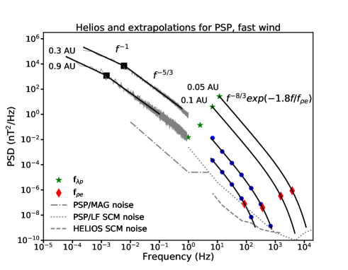
Figure 5: The complete turbulent spectrum from energy injection scales up to the sub-electron scales at 0.3 and 0.9 AU as measured by Helios. The energy containing scales (which correspond to $\sim f^{-1}$ spectrum) and the MHD inertial range ($\sim f^{-5/3}$) are covered by the Helios–MAG instrument (gray lines). The Helios–SCM instrument covers the kinetic scales (blue dots), studied in the present paper. The black solid lines indicate model functions $f^{-1}$, $f^{-5/3}$ and $f^{-8/3}\exp{(-1.8f/f_{\rho_{e}})}$ at different frequency ranges. The two most energetic spectra at high frequencies are the extrapolations of the kinetic spectrum in the fast wind that we expect to measure with PSP at 0.05 and 0.1 AU. The dashed line gives Helios-SCM noise, the dashed-dotted and dotted lines indicate noise levels of the different magnetic sensors on PSP. The Doppler shifted ion inertial length $\lambda_{p}$ (green stars) marks the transition from the inertial to the kinetic range; the electron Larmor radius $\rho_{e}$ (red diamonds) marks the dissipation cutoff.

Table 2: Mean plasma parameters at 4 radial distances from the Sun, corresponding to the spectra in Figure 5.

$R$ (AU)	0.9	0.3	0.1	0.05
$B_{0}$ (nT)	$7\pm 2$	$41\pm 3$	280	990
$V$ (km/s)	$705\pm 35$	$650\pm 40$	510	410
$n_{p}$ (cm-3)	$4\pm 1$	$31\pm 4$	350	1700
$T_{p}$ (eV)	$21\pm 5$	$50\pm 9$	120	230
$T_{e}$ (eV)	$9\pm 2$	$15\pm 2$	19	25
$T_{p\perp}$ (eV)	$24\pm 5$	$65\pm 10$	-	-
$T_{e\perp}$ (eV)	$7\pm 1$	$12\pm 1$	-	-
$\beta_{p}$	$0.8\pm 0.2$	$0.5\pm 0.1$	0.2	0.15
$\beta_{e}$	$0.2\pm 0.1$	$0.10\pm 0.02$	0.04	0.02
$\lambda_{p}$ (km)	$108\pm 14$	$39\pm 3$	12	6
$\rho_{p}$ (km)	$101\pm 31$	$28\pm 3$	6	2
$\lambda_{e}$ (km)	$2.5\pm 0.3$	$0.9\pm 0.1$	0.3	0.1
$\rho_{e}$ (km)	$1.3\pm 0.4$	$0.3\pm 0.02$	0.05	0.02
$f_{cp}$ (Hz)	$0.10\pm 0.03$	$0.6\pm 0.05$	4	15
$f_{\lambda p}$ (Hz)	$1.0\pm 0.1$	$2.6\pm 0.3$	7	12
$f_{\rho p}$ (Hz)	$1.1\pm 0.3$	$3.6\pm 0.5$	14	30
$f_{\lambda e}$ (Hz)	$44\pm 6$	$110\pm 10$	300	500
$f_{\rho e}$ (Hz)	$90\pm 30$	$360\pm 40$	1530	3800
$f_{ce}$ (Hz)	$200\pm 60$	$1150\pm 80$	7800	28000

Let us now put our observations in a more general context of the solar wind turbulence. Figure 5 shows a complete turbulent spectrum covering the energy containing scales ($\sim f^{-1}$ spectral range), the inertial range at MHD scales ($\sim f^{-5/3}$ range), and the kinetic scales, as observed at 0.3 and 0.9 AU by Helios in the fast wind. The mean plasma parameters for the time intervals used here are given in Table 2.

We expect that the spectral properties we observe are generic for plasma turbulence at sub-ion to electron scales. The two most energetic spectra at high frequencies in Figure 5 are the extrapolations of the kinetic spectrum that we expect to observe in the fast solar wind with PSP at 0.05 and 0.1 AU (see the Appendix for more details). Indeed, the beginning of this kinetic spectrum following an $f^{-8/3}$–law between $\sim 10$ and $100$ Hz was recently observed by PSP at 35.7 solar radii (0.166 AU) Bale and et al. [2019], Bowen et al. [2020]. Future PSP observations closer to the Sun will show how the empirical picture of the kinetic turbulence given here may change.

Appendix: Extrapolation of turbulent spectra closer to the Sun

To plot the extrapolations of the kinetic spectra at 0.05 and 0.1 AU in Figure 5, we assume that the turbulence level will increase together with the mean field, keeping $\delta B/B_{0}\sim\text{const}$, as observed in the solar wind, [e.g., Beinroth and Neubauer, 1981, Bourouaine et al., 2012]. In the inner heliosphere, where $\beta<1$, the end of the Kolmogorov scaling is expected to happen at the proton inertial length $\lambda_{p}$ [Bourouaine et al., 2012, Chen et al., 2014] (see green stars). The exponential falloff at the end of the electromagnetic cascade is defined by the local $\rho_{e}$, as we confirm in this study. To determine the Doppler shifted frequencies where $\lambda_{p}$ and $\rho_{e}$ will appear in the extrapolated spectra ($f_{\lambda p}=V/2\pi\lambda_{p}$ and $f_{\rho e}=V/2\pi\rho_{e}$), we use plasma parameters (proton density $n_{p}$, electron temperature $T_{e}$, magnetic field $B_{0}$, and solar wind speed $V$) extrapolated from the in-situ Helios measurements (from 0.3 to 0.9 AU). These latter extrapolations have been performed by connecting the gradient of the Helios density measurements to the one measured remotely from coronal white light eclipse observations. More precisely, we have retrieved the radial variations of both the electron density $n_{e}(R)$ (which we assume for simplicity to be equal to $n_{p}(R)$) and bulk speed $V(R)$ all the way down to the low corona by (i) imposing that the density matches both the 0.3 to 1 AU Helios density observations and the coronal density observations obtained remotely by Sittler and Guhathakurta [1999] and (ii) imposing the conservation of the mass flux $n_{e}(R)V(R)R^{2}=\text{const}$. The plasma parameters used for the extrapolated spectra as well as for the time intervals of the Helios measurements are summarized in Table 2.

Data

The Helios–1 data are available on the Helios data archive (http://helios-data.ssl.berkeley.edu/).

Software

The routine used to fit the data with the model, Eq.(1), is optimize.curve$\_$fit from scipy$/$python [Virtanen et al., 2020].

Correspondence

Correspondence should be addressed to O. Alexandrova (email: olga.alexandrova@obspm.fr).

References

- Alexandrova et al. [2008] O. Alexandrova, C. Lacombe, and A. Mangeney. Spectra and anisotropy of magnetic fluctuations in the Earth’s magnetosheath: Cluster observations. Annales Geophysicae, 26:3585–3596, November 2008.
- Alexandrova et al. [2009] O. Alexandrova, J. Saur, C. Lacombe, A. Mangeney, J. Mitchell, S. J. Schwartz, and P. Robert. Universality of Solar-Wind Turbulent Spectrum from MHD to Electron Scales. Phys. Rev. Lett., 103(16):165003–+, October 2009. doi: 10.1103/PhysRevLett.103.165003.
- Alexandrova et al. [2010] O. Alexandrova, J. Saur, C. Lacombe, A. Mangeney, S. J. Schwartz, J. Mitchell, R. Grappin, and P. Robert. Solar wind turbulent spectrum from MHD to electron scales. Twelfth International Solar Wind Conference, 1216:144–147, March 2010. doi: 10.1063/1.3395821.
- Alexandrova et al. [2012] O. Alexandrova, C. Lacombe, A. Mangeney, R. Grappin, and M. Maksimovic. Solar Wind Turbulent Spectrum at Plasma Kinetic Scales. ApJ, 760:121, December 2012. doi: 10.1088/0004-637X/760/2/121.
- Alexandrova et al. [2013] O. Alexandrova, C. H. K. Chen, L. Sorriso-Valvo, T. S. Horbury, and S. D. Bale. Solar Wind Turbulence and the Role of Ion Instabilities. Space Sci. Rev., 178:101–139, October 2013. doi: 10.1007/s11214-013-0004-8.
- Bale and et al. [2019] S. D. Bale and et al. Highly structured slow solar wind emerging from an equatorial coronal hole. Nature, 576:237–242, 2019. doi: 10.1038/s41586-019-1818-7.
- Bandyopadhyay et al. [2020] Riddhi Bandyopadhyay, Luca Sorriso-Valvo, Alexand ros Chasapis, Petr Hellinger, William H. Matthaeus, Andrea Verdini, Simone Landi, Luca Franci, Lorenzo Matteini, Barbara L. Giles, Daniel J. Gershman, Thomas E. Moore, Craig J. Pollock, Christopher T. Russell, Robert J. Strangeway, Roy B. Torbert, and James L. Burch. In Situ Observation of Hall Magnetohydrodynamic Cascade in Space Plasma. Phys. Rev. Lett., 124(22):225101, June 2020. doi: 10.1103/PhysRevLett.124.225101.
- Beinroth and Neubauer [1981] H. J. Beinroth and F. M. Neubauer. Properties of whistler mode waves between 0.3 and 1.0 AU from HELIOS observations. J. Geophys. Res., 86:7755–7760, September 1981. doi: 10.1029/JA086iA09p07755.
- Boldyrev [2005] S. Boldyrev. On the Spectrum of Magnetohydrodynamic Turbulence. ApJ, 626:L37–L40, June 2005. doi: 10.1086/431649.
- Bourouaine et al. [2012] S. Bourouaine, O. Alexandrova, E. Marsch, and M. Maksimovic. On Spectral Breaks in the Power Spectra of Magnetic Fluctuations in Fast Solar Wind between 0.3 and 0.9 AU. ApJ, 749:102, April 2012. doi: 10.1088/0004-637X/749/2/102.
- Bowen et al. [2020] Trevor A. Bowen, Alfred Mallet, Stuart D. Bale, J. W. Bonnell, Anthony W. Case, Benjamin D. G. Chandran, Alexandros Chasapis, Christopher H. K. Chen, Die Duan, Thierry Dudok de Wit, Keith Goetz, Jasper S. Halekas, Peter R. Harvey, J. C. Kasper, Kelly E. Korreck, Davin Larson, Roberto Livi, Robert J. MacDowall, David M. Malaspina, Michael D. McManus, Marc Pulupa, Michael Stevens, and Phyllis Whittlesey. Constraining Ion-Scale Heating and Spectral Energy Transfer in Observations of Plasma Turbulence. Phys. Rev. Lett., 125(2):025102, July 2020. doi: 10.1103/PhysRevLett.125.025102.
- Bruno and Carbone [2013] R. Bruno and V. Carbone. The Solar Wind as a Turbulence Laboratory. Living Reviews in Solar Physics, 10:2, May 2013. doi: 10.12942/lrsp-2013-2.
- Chandran et al. [2015] B. D. G. Chandran, A. A. Schekochihin, and A. Mallet. Intermittency and Alignment in Strong RMHD Turbulence. ApJ, 807:39, July 2015. doi: 10.1088/0004-637X/807/1/39.
- Chen [2016] C. H. K. Chen. Recent progress in astrophysical plasma turbulence from solar wind observations. Journal of Plasma Physics, 82(6):535820602, Dec 2016. doi: 10.1017/S0022377816001124.
- Chen et al. [2010] C. H. K. Chen, R. T. Wicks, T. S. Horbury, and A. A. Schekochihin. Interpreting Power Anisotropy Measurements in Plasma Turbulence. ApJ, 711:L79–L83, March 2010. doi: 10.1088/2041-8205/711/2/L79.
- Chen et al. [2014] C. H. K. Chen, L. Leung, S. Boldyrev, B. A. Maruca, and S. D. Bale. Ion-scale spectral break of solar wind turbulence at high and low beta. Geophys. Res. Lett., 41:8081–8088, November 2014. doi: 10.1002/2014GL062009.
- Chen et al. [2020] C. H. K. Chen, S. D. Bale, J. W. Bonnell, D. Borovikov, T. A. Bowen, D. Burgess, A. W. Case, B. D. G. Chandran, T. Dudok de Wit, K. Goetz, P. R. Harvey, J. C. Kasper, K. G. Klein, K. E. Korreck, D. Larson, R. Livi, R. J. MacDowall, D. M. Malaspina, A. Mallet, M. D. McManus, M. Moncuquet, M. Pulupa, M. L. Stevens, and P. Whittlesey. The Evolution and Role of Solar Wind Turbulence in the Inner Heliosphere. ApJS, 246(2):53, February 2020. doi: 10.3847/1538-4365/ab60a3.
- Chen et al. [1993] S. Chen, G. Doolen, J. R. Herring, R. H. Kraichnan, S. A. Orszag, and Z. S. She. Far-dissipation range of turbulence. Physical Review Letters, 70:3051–3054, May 1993. doi: 10.1103/PhysRevLett.70.3051.
- Coleman [1968] P. J. Coleman, Jr. Turbulence, Viscosity, and Dissipation in the Solar-Wind Plasma. ApJ, 153:371, August 1968. doi: 10.1086/149674.
- Cornilleau-Wehrlin et al. [1997] N. Cornilleau-Wehrlin, P. Chauveau, S. Louis, A. Meyer, J. M. Nappa, S. Perraut, L. Rezeau, P. Robert, A. Roux, C. de Villedary, Y. de Conchy, L. Friel, C. C. Harvey, D. Hubert, C. Lacombe, R. Manning, F. Wouters, F. Lefeuvre, M. Parrot, J. L. Pincon, B. Poirier, W. Kofman, and P. Louarn. The Cluster Spatio-Temporal Analysis of Field Fluctuations (STAFF) Experiment. Space Sci. Rev., 79:107–136, January 1997. doi: 10.1023/A:1004979209565.
- Denskat et al. [1983] K. U. Denskat, H. J. Beinroth, and F. M. Neubauer. Interplanetary magnetic field power spectra with frequencies from 2.4 X 10 to the -5th HZ to 470 HZ from HELIOS-observations during solar minimum conditions. Journal of Geophysics Zeitschrift Geophysik, 54:60–67, 1983.
- Escoubet et al. [1997] C. P. Escoubet, R. Schmidt, and M. L. Goldstein. Cluster - Science and Mission Overview. Space Sci. Rev., 79:11–32, January 1997. doi: 10.1023/A:1004923124586.
- Frisch [1995] U. Frisch. Turbulence: The Legacy of A. N. Kolmogorov. Cambridge University Press, Cambridge (UK), 1995.
- Goldreich and Sridhar [1995] P. Goldreich and S. Sridhar. Toward a theory of interstellar turbulence. II. Strong Alfvénic turbulence. ApJ, 438:763–775, January 1995. doi: 10.1086/175121.
- Greco et al. [2016] A. Greco, S. Perri, S. Servidio, E. Yordanova, and P. Veltri. The Complex Structure of Magnetic Field Discontinuities in the Turbulent Solar Wind. ApJ, 823:L39, June 2016. doi: 10.3847/2041-8205/823/2/L39.
- Hellinger et al. [2018] Petr Hellinger, Andrea Verdini, Simone Landi, Luca Franci, and Lorenzo Matteini. von Kármán-Howarth Equation for Hall Magnetohydrodynamics: Hybrid Simulations. ApJ, 857(2):L19, April 2018. doi: 10.3847/2041-8213/aabc06.
- Howes et al. [2011] G. G. Howes, J. M. Tenbarge, and W. Dorland. A weakened cascade model for turbulence in astrophysical plasmas. Physics of Plasmas, 18(10):102305, October 2011. doi: 10.1063/1.3646400.
- Jagarlamudi et al. [2020] Vamsee Krishna Jagarlamudi, Olga Alexandrova, Laura Berčič, Thierry Dudok de Wit, Vladimir Krasnoselskikh, Milan Maksimovic, and Štěpán Štverák. Whistler Waves and Electron Properties in the Inner Heliosphere: Helios Observations. ApJ, 897(2):118, July 2020. doi: 10.3847/1538-4357/ab94a1.
- Kiyani et al. [2013] K. H. Kiyani, S. C. Chapman, F. Sahraoui, B. Hnat, O. Fauvarque, and Y. V. Khotyaintsev. Enhanced Magnetic Compressibility and Isotropic Scale Invariance at Sub-ion Larmor Scales in Solar Wind Turbulence. ApJ, 763:10, January 2013. doi: 10.1088/0004-637X/763/1/10.
- Kiyani et al. [2015] K. H. Kiyani, K. T. Osman, and S. C. Chapman. Dissipation and heating in solar wind turbulence: From the macro to the micro and back again. Philosophical Transactions of the Royal Society of London Series A, 373(2041):20140155–20140155, Apr 2015. doi: 10.1098/rsta.2014.0155.
- Lacombe et al. [2014] C. Lacombe, O. Alexandrova, L. Matteini, O. Santolík, N. Cornilleau-Wehrlin, A. Mangeney, Y. de Conchy, and M. Maksimovic. Whistler Mode Waves and the Electron Heat Flux in the Solar Wind: Cluster Observations. ApJ, 796:5, November 2014. doi: 10.1088/0004-637X/796/1/5.
- Lacombe et al. [2017] C. Lacombe, O. Alexandrova, and L. Matteini. Anisotropies of the Magnetic Field Fluctuations at Kinetic Scales in the Solar Wind: Cluster Observations. ApJ, 848:45, October 2017. doi: 10.3847/1538-4357/aa8c06.
- Li et al. [2019] Tak Chu Li, Gregory G. Howes, Kristopher G. Klein, Yi-Hsin Liu, and Jason M. Tenbarge. Collisionless energy transfer in kinetic turbulence: field-particle correlations in Fourier space. Journal of Plasma Physics, 85(4):905850406, August 2019. doi: 10.1017/S0022377819000515.
- Mangeney et al. [2006] A. Mangeney, C. Lacombe, M. Maksimovic, A. A. Samsonov, N. Cornilleau-Wehrlin, C. C. Harvey, J.-M. Bosqued, and P. Trávníček. Cluster observations in the magnetosheath - Part 1: Anisotropies of the wave vector distribution of the turbulence at electron scales. Annales Geophysicae, 24:3507–3521, December 2006. doi: 10.5194/angeo-24-3507-2006.
- Matteini et al. [2017] L. Matteini, O. Alexandrova, C. H. K. Chen, and C. Lacombe. Electric and magnetic spectra from MHD to electron scales in the magnetosheath. Mon. Notices R. Astron. Soc., 466:945–951, April 2017. doi: 10.1093/mnras/stw3163.
- Matthaeus et al. [2008] W. H. Matthaeus, S. Servidio, and P. Dmitruk. Comment on “Kinetic Simulations of Magnetized Turbulence in Astrophysical Plasmas”. Phys. Rev. Lett., 101:149501, 2008. doi: 10.1103/PhysRevLett.101.149501.
- Meyer-Vernet [2007] N. Meyer-Vernet. Basics of the Solar Wind. Cambridge University Press, 2007.
- Neubauer et al. [1977a] F. M. Neubauer, H. J. Beinroth, H. Barnstorf, and G. Dehmel. Initial results from the Helios-1 search-coil magnetometer experiment. Journal of Geophysics Zeitschrift Geophysik, 42:599–614, 1977a.
- Neubauer et al. [1977b] F. M. Neubauer, G. Musmann, and G. Dehmel. Fast magnetic fluctuations in the solar wind - HELIOS I. J. Geophys. Res., 82:3201–3212, August 1977b. doi: 10.1029/JA082i022p03201.
- Note [1] Note1. One astronomical unit (AU) is the distance from Earth to the Sun, which is about m.
- Note [2] Note2. The Geocentric Solar Ecliptic (GSE) frame has its -axis pointing from the Earth towards the Sun, the -axis is chosen to be in the ecliptic plane pointing towards dusk (thus opposing planetary motion), -axis is normal to the ecliptic plane, northwards.
- Oughton and Matthaeus [2020] S. Oughton and W. H. Matthaeus. Critical balance and the physics of magnetohydrodynamic turbulence. The Astrophysical Journal, 897(1):37, jun 2020. doi: 10.3847/1538-4357/ab8f2a. URL https://doi.org/10.3847%2F1538-4357%2Fab8f2a.
- Oughton et al. [1994] S. Oughton, E. R. Priest, and W. H. Matthaeus. The influence of a mean magnetic field on three-dimensional magnetohydrodynamic turbulence. Journal of Fluid Mechanics, 280:95–117, 1994. doi: 10.1017/S0022112094002867.
- Papini et al. [2019] E. Papini, L. Franci, S. Landi, A. Verdini, L. Matteini, and P. Hellinger. Can Hall magnetohydrodynamics explain plasma turbulence at sub-ion scales? Astrophys. J., 870:52, 2019. doi: 10.3847/1538-4357/aaf003.
- Parashar et al. [2018] Tulasi N. Parashar, William H. Matthaeus, and Michael A. Shay. Dependence of Kinetic Plasma Turbulence on Plasma . Astrophys. J. Lett., 864:L21, 2018. doi: 10.3847/2041-8213/aadb8b.
- Passot and Sulem [2015] T. Passot and P. L. Sulem. A Model for the Non-universal Power Law of the Solar Wind Sub-ion-scale Magnetic Spectrum. ApJ, 812(2):L37, October 2015. doi: 10.1088/2041-8205/812/2/L37.
- Perri et al. [2012] S. Perri, M. L. Goldstein, J. C. Dorelli, and F. Sahraoui. Detection of Small-Scale Structures in the Dissipation Regime of Solar-Wind Turbulence. Physical Review Letters, 109(19):191101, November 2012. doi: 10.1103/PhysRevLett.109.191101.
- Roberts et al. [2017] O. W. Roberts, O. Alexandrova, P. Kajdič, L. Turc, D. Perrone, C. P. Escoubet, and A. Walsh. Variability of the Magnetic Field Power Spectrum in the Solar Wind at Electron Scales. ApJ, 850:120, December 2017. doi: 10.3847/1538-4357/aa93e5.
- Rudakov et al. [2011] L. Rudakov, M. Mithaiwala, G. Ganguli, and C. Crabtree. Linear and nonlinear Landau resonance of kinetic Alfvén waves: Consequences for electron distribution and wave spectrum in the solar wind. Physics of Plasmas, 18(1):012307, January 2011. doi: 10.1063/1.3532819.
- Sahraoui et al. [2010] F. Sahraoui, M. L. Goldstein, G. Belmont, P. Canu, and L. Rezeau. Three Dimensional Anisotropic k Spectra of Turbulence at Subproton Scales in the Solar Wind. Phys. Rev. Lett., 105:131101–+, September 2010.
- Sahraoui et al. [2013] F. Sahraoui, S. Y. Huang, G. Belmont, M. L. Goldstein, A. Rétino, P. Robert, and J. De Patoul. Scaling of the Electron Dissipation Range of Solar Wind Turbulence. ApJ, 777:15, November 2013. doi: 10.1088/0004-637X/777/1/15.
- Salem et al. [2003] C. Salem, D. Hubert, C. Lacombe, S. D. Bale, A. Mangeney, D. E. Larson, and R. P. Lin. Electron properties and coulomb collisions in the solar wind at 1 AU:WindObservations. The Astrophysical Journal, 585(2):1147–1157, mar 2003. doi: 10.1086/346185. URL https://doi.org/10.1086%2F346185.
- Schreiner and Saur [2017] A. Schreiner and J. Saur. A Model for Dissipation of Solar Wind Magnetic Turbulence by Kinetic Alfvén Waves at Electron Scales: Comparison with Observations. ApJ, 835:133, February 2017. doi: 10.3847/1538-4357/835/2/133.
- Shebalin et al. [1983] J. V. Shebalin, W. H. Matthaeus, and D. Montgomery. Anisotropy in MHD turbulence due to a mean magnetic field. Journal of Plasma Physics, 29:525–547, June 1983.
- Sittler and Guhathakurta [1999] Jr. Sittler, Edward C. and Madhulika Guhathakurta. Semiempirical Two-dimensional MagnetoHydrodynamic Model of the Solar Corona and Interplanetary Medium. ApJ, 523(2):812–826, October 1999. doi: 10.1086/307742.
- Štverák et al. [2008] Š. Štverák, P. Trávníček, M. Maksimovic, E. Marsch, A. Fazakerley, and E. E. Scime. Electron temperature anisotropy constraints in the solar wind. J. Geophys. Res., 113:A03103, 2008. doi: 10.1029/2007JA012733.
- TenBarge et al. [2013] J. M. TenBarge, G. G. Howes, and W. Dorland. Collisionless Damping at Electron Scales in Solar Wind Turbulence. ApJ, 774(2):139, September 2013. doi: 10.1088/0004-637X/774/2/139.
- Verdini et al. [2015] Andrea Verdini, Roland Grappin, Petr Hellinger, Simone Land i, and Wolf Christian Müller. Anisotropy of Third-order Structure Functions in MHD Turbulence. ApJ, 804(2):119, May 2015. doi: 10.1088/0004-637X/804/2/119.
- Virtanen et al. [2020] Pauli Virtanen, Ralf Gommers, Travis E. Oliphant, Matt Haberland, Tyler Reddy, David Cournapeau, Evgeni Burovski, Pearu Peterson, Warren Weckesser, Jonathan Bright, Stéfan J. van der Walt, Matthew Brett, Joshua Wilson, K. Jarrod Millman, Nikolay Mayorov, Andrew R. J. Nelson, Eric Jones, Robert Kern, Eric Larson, C J Carey, İlhan Polat, Yu Feng, Eric W. Moore, Jake VanderPlas, Denis Laxalde, Josef Perktold, Robert Cimrman, Ian Henriksen, E. A. Quintero, Charles R. Harris, Anne M. Archibald, Antônio H. Ribeiro, Fabian Pedregosa, Paul van Mulbregt, and SciPy 1.0 Contributors. SciPy 1.0: Fundamental Algorithms for Scientific Computing in Python. Nature Methods, 17:261–272, 2020. doi: 10.1038/s41592-019-0686-2.