Primordial Black Hole Formation in Non-Minimal Curvaton Scenario
Abstract
In the curvaton scenario, the curvature perturbation is generated after inflation at the curvaton decay, which may have a prominent non-Gaussian effect. For a model with a non-trivial kinetic term, an enhanced curvature perturbation on a small scale can be realized, which can lead to copious production of primordial black holes (PBHs) and induce secondary gravitational waves (GWs). Using the probability distribution function (PDF) which takes full nonlinear effects into account, we calculate the PBH formation. We find that under the assumption that thus formed PBHs would not overclose the universe, the non-Gaussianity of the curvature perturbation can be well approximated by the local quadratic form, which can be used to calculate the induced GWs. In this model the limit of large non-Gaussianity can be reached when the curvaton energy fraction is small at the moment of curvaton decay. We also show that in the limit the PDF is similar to that of ultraslow-roll inflation.
Introduction.—The discovery of gravitational waves (GWs) by LIGO in 2015 marked the dawn of GW cosmology Abbott et al. (2016). Since then about 90 GW events have been detected Abbott et al. (2021a). Besides the transient GWs emitted from mergers, the stochastic GW background is an important scientific target of LIGO/VIRGO/KAGRA Abbott et al. (2021b) and the space-borne interferometers like LISA Barausse et al. (2020), Taiji Hu and Wu (2017); Ruan et al. (2020), and TianQin Luo et al. (2016). Among all the sources of stochastic GWs, secondary GWs induced by a peaked primordial curvature perturbation Matarrese et al. (1993, 1994, 1998); Noh and Hwang (2004); Carbone and Matarrese (2005); Nakamura (2007); Ananda et al. (2007); Osano et al. (2007); Baumann et al. (2007) have recently attracted much attention Assadullahi and Wands (2010); Alabidi et al. (2012, 2013); Biagetti et al. (2015); Inomata et al. (2017a); Nakama et al. (2017); Orlofsky et al. (2017); Di and Gong (2018); Garcia-Bellido et al. (2017); Kohri and Terada (2018); Cai et al. (2019a); Bartolo et al. (2019); Unal (2019); Adshead et al. (2021); Yuan and Huang (2021); Pi and Sasaki (2020); Domènech (2021); Liu et al. (2021) as they imply the existence of abundant primordial black holes (PBHs) Saito and Yokoyama (2009, 2010); Bugaev and Klimai (2010, 2011). PBHs can play a number of important roles in cosmology. They may provide the seeds for galaxy formation Bean and Magueijo (2002); Kawasaki et al. (2012); Nakama et al. (2018); Carr and Silk (2018); Nakama et al. (2019); Carr et al. (2021a); Atal et al. (2020a), may account for a population of the LIGO-Virgo events Bird et al. (2016); Clesse and García-Bellido (2017); Sasaki et al. (2016); Blinnikov et al. (2016); Ali-Haïmoud and Kamionkowski (2017); Zumalacarregui and Seljak (2018); Garcia-Bellido et al. (2018); Wong et al. (2021); Hütsi et al. (2021); Kimura et al. (2021); Franciolini et al. (2021), the ultra-short timescale microlensing events Mróz et al. (2017); Niikura et al. (2019a), the planet 9 Scholtz and Unwin (2020), hot spot for baryogenesis Byrnes et al. (2018); Carr et al. (2021b); García-Bellido et al. (2019); Carr et al. (2019); De Luca et al. (2021), and the cold dark matter Carr et al. (2016); Niikura et al. (2019b); Katz et al. (2018, 2018); Montero-Camacho et al. (2019); Sugiyama et al. (2020); Laha (2019); DeRocco and Graham (2019). In the last case, the curvature perturbation on uniform density slices should be enhanced to at , which can be realized by, for instance, ultra-slow-roll single-field inflation Yokoyama (1998); Garcia-Bellido et al. (2016); Cheng et al. (2017); Garcia-Bellido and Ruiz Morales (2017); Cheng et al. (2018); Dalianis et al. (2019); Tada and Yokoyama (2019); Xu et al. (2020); Mishra and Sahni (2020); Bhaumik and Jain (2020); Liu et al. (2020); Atal et al. (2020b); Fu et al. (2020a); Vennin (2020); Ragavendra et al. (2021); Gao and Yang (2021); Pattison et al. (2021); Ng and Wu (2021), modified gravity Kannike et al. (2017); Pi et al. (2018); Gao and Guo (2018); Cheong et al. (2021, 2020); Fu et al. (2019); Dalianis et al. (2020); Lin et al. (2020); Fu et al. (2020b); Aldabergenov et al. (2020, 2021); Yi et al. (2021); Gao et al. (2020); Dalianis and Kritos (2021); Kawai and Kim (2021), multi-field inflation with a flat potential Garcia-Bellido et al. (1996); Kawasaki et al. (1998); Frampton et al. (2010); Clesse and García-Bellido (2015); Inomata et al. (2017b, 2018); Espinosa et al. (2018); Kawasaki et al. (2020); Palma et al. (2020); Fumagalli et al. (2020); Braglia et al. (2020); Anguelova (2021); Romano (2020); Gundhi and Steinwachs (2021); Gundhi et al. (2021), resonance Cai et al. (2018a); Chen et al. (2020); Cai et al. (2019b, 2020, 2021a, 2021b), oscillons Cotner and Kusenko (2017a, b); Cotner et al. (2018, 2019), etc.
In this paper we propose a non-minimal curvaton model that can produce such an enhanced, peaked curvature perturbation at . In the curvaton scenario, the primordial curvature perturbation is produced by the curvaton field perturbation that was isocurvature during inflation but turns into the curvature perturbation as the curvaton starts to dominate the universe Moroi and Takahashi (2001); Enqvist and Sloth (2002); Lyth et al. (2003). A simple mechanism to generate a peaked spectrum is to introduce a non-trivial field metric which suppresses the curvaton kinetic term around . The curvature perturbation produced by curvaton is intrinsically non-Gaussian Bartolo et al. (2004); Enqvist and Nurmi (2005); Sasaki et al. (2006). Using the probability distribution function which takes full nonlinear effects into account, we calculate the PBH formation. We find that under the assumption that the mean square value of is small, , which is justified a posteriori by the condition that the produced PBHs would not overclose the universe, the resultant fully nonlinear curvature perturbation can be well described by the quadratic local non-Gaussianity, , where is inversely proportional to the curvaton energy fraction at its decay moment, which can freely be very large.
Non-minimal Curvaton.— We consider a two-field theory with a non-trivial field metric,
| (1) |
where is the inflaton, is its potential, and is the curvaton with mass . Such a field metric may appear in dilatonic or axionic models or in modified gravity Berkin and Maeda (1991); Domènech and Sasaki (2015). We assume single-field slow-roll inflation with the energy density dominated by . The background field equations are
| (2) | |||
| (3) |
where is the Hubble parameter during inflation. The approximation in (2) holds because the curvaton is effectively “frozon” as we assume . The equation of motion for the curvaton perturbation on the spatially-flat slicing, , is
| (4) |
where we neglected the terms proportional to . Deep inside the horizon, the WKB solution to (4) for the initial conditions in the adiabatic vacuum is
| (5) |
On superhorizon scales, the -term in (4) is negligible. So (3) and (4) have the same form, which gives , and
| (6) |
for where is the horizon crossing time determined by . Thus the power spectrum of on the spatially-flat slicing is
| (7) |
We assume there is a sharp dip in which results in a peak in at . Around the peak, and are only very slowly varying. Hence their -dependence may be neglected. For sufficiently far away from , the right-hand side of (7) is slowly varying in , which results in an almost scale-invariant spectrum of .
After inflation, the universe is radiation-dominated with its energy density behaves as . After the Hubble expansion rate drops below , the curvaton begins to oscillate, and the energy density starts to behave as . The curvature perturbation on the uniform-curvaton-density slice is Lyth et al. (2005)
| (8) |
where and are the curvature perturbation and the “background” energy density of respectively, in an arbitrary gauge of . We have
| (9) |
where is a fiducial value of , and . In spatially-flat slicing, (8) becomes , where is the curvaton contrast in the spatially-flat slicing, and . In uniform-total-density slicing, (8) becomes , which gives . is the “bare” curvature perturbation defined by choosing the time slicing on the right hand side of (8) to be of uniform total-density, which has nonzero mean value and will be renormalized to when we discuss the PBH formation later. Similarly for the radiation we have . The last step holds because we assume the curvature perturbation is mainly contributed by the curvaton, i.e., .
We adopt the sudden-decay approximation to calculate the curvature perturbation, which is in good agreement with the numerical results Malik and Lyth (2006). The curvaton decays when the Hubble rate equals to the decay rate on the hypersurface of uniform-total-density,
| (10) |
Then at we have
| (11) |
where
| (12) | ||||
| (13) |
After the decay, , is conserved until it reenters the Hubble horizon. Eq. (11) is a fourth order algebraic equation for , with the real positive solution given by Sasaki et al. (2006)
| (14) |
where
| (15) | ||||
| (16) |
As we commented, “physical” curvature perturbation should be defined as .
When is small, (14) can be expanded as
| (17) |
To the second order has the familiar form of the quadratic local non-Gaussianity,
| (18) |
with and . We will see that (18) is a good approximation if we require that PBHs do not overclose the universe.
| (19) |
where . The ensemble average is calculated by , where is the Gaussian probability distribution function (PDF) of ,
| (20) |
is the variance of smoothed on scale , i.e., . Therefore, the leading order of (17), , gives , which can be checked a posteriori.
In momentum space, is connected to the power spectrum of in (7) as
| (21) |
is the Fourier transform of a window function in real space, used for smoothing. There are some ambiguities in the choice of window functions Young (2019); Tokeshi et al. (2020). For concreteness and simplicity, we choose the Gaussian window function, whose Fourier transform is . As mentioned before, and depend only weakly on , while has a sharp dip at . A dip in gives a peak in in (21). So the power spectrum in (21) can be modeled by a lognormal function with the dimensionless width ,
| (22) |
We have neglected the near-scale-invariant component which is much smaller than the peak component. For simplicity, we focus on a narrow peak, . Then the smoothed variance of the curvaton contrast in (21) is , where is the total power of .
PBHs and Induced GWs.—Large density contrast may cause the PBH formation at the horizon reentry. The density contrast on the comoving slicing is
| (23) |
where and are the curvature perturbations in the longitudinal and uniform-total-density slicings, respectively, which are related to each other as on superhorizon scales in the radiation-dominated era Kodama and Sasaki (1984). The difficulty is that the operation is nonlocal when transforming the criterion for to that for , . Nevertheless, when the peak of at is narrow, we may replace the gradient operator by . Therefore, the inverse of (23) can be converted to an algebraic relation, , where is the comoving horizon scale, which is also the smoothing scale. From (19) with , we have
| (24) |
The PDF of is now related to that of the curvaton contrast as
| (25) |
The PBH abundance can be calculated by integrating the smoothed PDF of from its critical value , à la Press-Schechter,
| (26) |
where is the complementary error function and the critical values are given by (24) with . The critical comoving density contrast varies from 0.2 to 0.6 in the literature. In this paper we adopt the value of inferred from the optimized criterion given in Yoo et al. (2018), where the peak theory is used to determine the critical peak value of , for a specific profile in real space. Translating this result into the Press-Schechter language, the corresponding value is estimated as .
The -dependence of can be converted to the PBH mass dependence by , where is the PBH mass when reenters the horizon. Fig. 1 shows with fixed PBH abundance today. The width of the peak is , independent of and , reflecting the the fact that the width of is small, .
The PBH abundance we observe today is parameterized by , which is connected to by Carr et al. (2020)
| (27) |
where . The equal- contours in the -plane are shown in Fig. 2. For , depends only on the combination , which can be fitted by
| (28) |
The smoothed variance of can be calculated by the PDF of ,
| (29) |
where is the bare curvature perturbation defined in (14) as a function of . The total power is given by the limit of (29). When , can be approximated by (17),
| (30) |
which is in the form of a quadratic local non-Gaussianity. Substituting (30) into (29), we have
| (31) |
(31) fits the numerical result quite well when , shown in Fig. 2. As and depends only on when and , their contours are parallel to each other and the PBH abundance only depends on the amplitude of the power spectrum there.
In the vicinity of , we have from (11). Interestingly, this logarithmic form is the same as the fully nonlinear curvature perturbation generated in ultra-slow-roll inflation Cai et al. (2018b); Atal et al. ; Atal et al. (2020b), from which the PBH formation has been calculated by (25) in Ref.Biagetti et al. (2021). In our model, the full nonlinear region ( and ) produces too much PBHs and is of no cosmological interest.
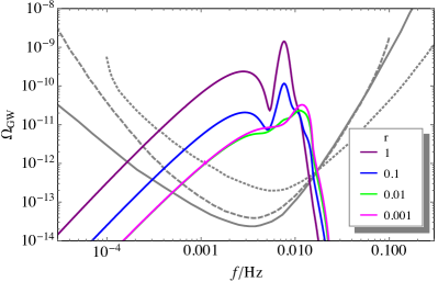
If the PBHs do not overclose our universe, i.e., if the energy density of PBHs is smaller than the critical density today, can be well approximated by the quadratic local non-Gaussian form , with and . This implies that the power spectrum of consists of the Gaussian component and the non-Gaussian component given by convolution of two Gaussian spectra. The power spectrum determines the Gaussian component of the curvature perturbation spectrum, , while the non-Gaussian component is the convolution of . The induced GWs can be calculated by following the computations for the quadratic local non-Gaussianity case Cai et al. (2019a); Unal (2019); Adshead et al. (2021). The resultant GW spectrum is shown in Fig. 3 for at , with the width . The peak amplitude of the induced GW is roughly times the square of the curvature perturbation spectrum at the peak Pi and Sasaki (2020); Domènech (2021). As is shown in Fig. 2, if the PBH abundance is fixed, as well as decreases as decreases, but levels off to a constant as . This is because both and depend only on the combination in this limit. In the asteroid-mass window, PBHs can be all the dark matter, which requires from (28). The associated induced GW spectrum reaches its maximum,
| (32) |
at Hz. This is the lower bound of when . As is shown in Fig. 3, (32) is well above the power-law integrated sensitivity curves of LISA, Taiji, and TianQin around Hz. So we reach the conclusion that the induced GWs must be detectable by LISA (and/or other planned space interferometeric observatories like Taiji/TianQin/BBO/DECIGO), if PBHs formed from the peaked curvature perturbation in the curvaton scenario constitute all the dark matter. This conclusion is in complete agreement with Cai et al. (2019a), where the quadratic local non-Gaussianity is assumed a priori rather than derived. Here we have shown that the non-Gaussianity in the curvaton scenario can be well described by the quadratic form as long as we focus on the parameters of cosmological interest.
Conclusion.—Based on the curvaton scenario with a non-trivial field metric, we constructed a mechanism to enhance the curvature perturbation on small scales. The resulting curvature perturbation is fully non-Gaussian, while we use the probability distribution function to calculate the PBH formation with all the nonlinear effects taken into account. The PBH formation in curvaton scenario based on the expansion series of the curvature perturbation up to quadratic order has been studied before Kawasaki et al. (2013); Firouzjahi et al. (2013); Kohri et al. (2013); Bugaev and Klimai (2013); Young and Byrnes (2013); Ando et al. (2018a, b); Chen and Cai (2019); Inomata et al. (2021); Liu and Xu (2021), but our paper is the first to study the PBH formation for the fully nonliear curvature perturbation.
Once we focus on the parameter space of cosmological interest, amazingly the curvature perturbation can be well approximated by a quadratic local non-Gaussianity . In this form the nonlinear parameter can freely go to very large values, which is impossible in an expansion series. We further calculate the energy spectrum of the concomitant induced GWs under this approximation. Due to the enhancement of the PBH abundance by the non-Gaussianity, the power spectrum of the curvature perturbation required to generate a fixed amount of PBHs is suppressed when the non-Gaussianity is large. Yet the suppression has a lower bound when . For PBHs to be all the dark matter, we have and , which must be detectable by the planned interferometeric GW detectors in space.
In the region of and , the quadratic approximation breaks down and all the higher order terms should be taken into account. They sum up to be the similar logarithmic form to that in the ultra-slow-roll inflation Atal et al. ; Atal et al. (2020b); Kitajima et al. (2021); Biagetti et al. (2021); Escrivà et al. (2022); Pi and Sasaki (2023), as . Assuming the PDF of is Gaussian, this gives a non-Gaussian exponential tail of the PDF for the PBH formation. We leave the connection of these two models for future work.
Acknowledgements.
Acknowledgement.—The work of S.P. is supported by the National Key Research and Development Program of China Grant No. 2021YFC2203004, by Project 12047503 of the National Natural Science Foundation of China, by JSPS Grant-in-Aid for Early-Career Scientists No. JP20K14461, and in part by the International Centre for Theoretical Sciences (ICTS) for the online program – ICTS Summer School on Gravitational-Wave Astronomy (code: ICTS/gws2021/7). This work is also supported in part by the JSPS KAKENHI Nos. JP19H01895, JP20H04727, and JP20H05853, and in part by the World Premier International Research Center Initiative (WPI Initiative), MEXT, Japan.References
- Abbott et al. (2016) B. P. Abbott et al. (LIGO Scientific, Virgo), Phys. Rev. Lett. 116, 061102 (2016), arXiv:1602.03837 [gr-qc] .
- Abbott et al. (2021a) R. Abbott et al. (LIGO Scientific, VIRGO, KAGRA), (2021a), arXiv:2111.03606 [gr-qc] .
- Abbott et al. (2021b) R. Abbott et al. (KAGRA, Virgo, LIGO Scientific), Phys. Rev. D 104, 022004 (2021b), arXiv:2101.12130 [gr-qc] .
- Barausse et al. (2020) E. Barausse et al., Gen. Rel. Grav. 52, 81 (2020), arXiv:2001.09793 [gr-qc] .
- Hu and Wu (2017) W.-R. Hu and Y.-L. Wu, Natl. Sci. Rev. 4, 685 (2017).
- Ruan et al. (2020) W.-H. Ruan, Z.-K. Guo, R.-G. Cai, and Y.-Z. Zhang, Int. J. Mod. Phys. A 35, 2050075 (2020), arXiv:1807.09495 [gr-qc] .
- Luo et al. (2016) J. Luo et al. (TianQin), Class. Quant. Grav. 33, 035010 (2016), arXiv:1512.02076 [astro-ph.IM] .
- Matarrese et al. (1993) S. Matarrese, O. Pantano, and D. Saez, Phys. Rev. D 47, 1311 (1993).
- Matarrese et al. (1994) S. Matarrese, O. Pantano, and D. Saez, Phys. Rev. Lett. 72, 320 (1994), arXiv:astro-ph/9310036 .
- Matarrese et al. (1998) S. Matarrese, S. Mollerach, and M. Bruni, Phys. Rev. D 58, 043504 (1998), arXiv:astro-ph/9707278 .
- Noh and Hwang (2004) H. Noh and J.-c. Hwang, Phys. Rev. D 69, 104011 (2004).
- Carbone and Matarrese (2005) C. Carbone and S. Matarrese, Phys. Rev. D 71, 043508 (2005), arXiv:astro-ph/0407611 .
- Nakamura (2007) K. Nakamura, Prog. Theor. Phys. 117, 17 (2007), arXiv:gr-qc/0605108 .
- Ananda et al. (2007) K. N. Ananda, C. Clarkson, and D. Wands, Phys. Rev. D 75, 123518 (2007), arXiv:gr-qc/0612013 .
- Osano et al. (2007) B. Osano, C. Pitrou, P. Dunsby, J.-P. Uzan, and C. Clarkson, JCAP 04, 003 (2007), arXiv:gr-qc/0612108 .
- Baumann et al. (2007) D. Baumann, P. J. Steinhardt, K. Takahashi, and K. Ichiki, Phys. Rev. D 76, 084019 (2007), arXiv:hep-th/0703290 .
- Assadullahi and Wands (2010) H. Assadullahi and D. Wands, Phys. Rev. D 81, 023527 (2010), arXiv:0907.4073 [astro-ph.CO] .
- Alabidi et al. (2012) L. Alabidi, K. Kohri, M. Sasaki, and Y. Sendouda, JCAP 09, 017 (2012), arXiv:1203.4663 [astro-ph.CO] .
- Alabidi et al. (2013) L. Alabidi, K. Kohri, M. Sasaki, and Y. Sendouda, JCAP 05, 033 (2013), arXiv:1303.4519 [astro-ph.CO] .
- Biagetti et al. (2015) M. Biagetti, E. Dimastrogiovanni, M. Fasiello, and M. Peloso, JCAP 04, 011 (2015), arXiv:1411.3029 [astro-ph.CO] .
- Inomata et al. (2017a) K. Inomata, M. Kawasaki, K. Mukaida, Y. Tada, and T. T. Yanagida, Phys. Rev. D 95, 123510 (2017a), arXiv:1611.06130 [astro-ph.CO] .
- Nakama et al. (2017) T. Nakama, J. Silk, and M. Kamionkowski, Phys. Rev. D 95, 043511 (2017), arXiv:1612.06264 [astro-ph.CO] .
- Orlofsky et al. (2017) N. Orlofsky, A. Pierce, and J. D. Wells, Phys. Rev. D 95, 063518 (2017), arXiv:1612.05279 [astro-ph.CO] .
- Di and Gong (2018) H. Di and Y. Gong, JCAP 07, 007 (2018), arXiv:1707.09578 [astro-ph.CO] .
- Garcia-Bellido et al. (2017) J. Garcia-Bellido, M. Peloso, and C. Unal, JCAP 09, 013 (2017), arXiv:1707.02441 [astro-ph.CO] .
- Kohri and Terada (2018) K. Kohri and T. Terada, Phys. Rev. D 97, 123532 (2018), arXiv:1804.08577 [gr-qc] .
- Cai et al. (2019a) R.-g. Cai, S. Pi, and M. Sasaki, Phys. Rev. Lett. 122, 201101 (2019a), arXiv:1810.11000 [astro-ph.CO] .
- Bartolo et al. (2019) N. Bartolo, V. De Luca, G. Franciolini, M. Peloso, D. Racco, and A. Riotto, Phys. Rev. D 99, 103521 (2019), arXiv:1810.12224 [astro-ph.CO] .
- Unal (2019) C. Unal, Phys. Rev. D 99, 041301 (2019), arXiv:1811.09151 [astro-ph.CO] .
- Adshead et al. (2021) P. Adshead, K. D. Lozanov, and Z. J. Weiner, JCAP 10, 080 (2021), arXiv:2105.01659 [astro-ph.CO] .
- Yuan and Huang (2021) C. Yuan and Q.-G. Huang, Phys. Lett. B 821, 136606 (2021), arXiv:2007.10686 [astro-ph.CO] .
- Pi and Sasaki (2020) S. Pi and M. Sasaki, JCAP 09, 037 (2020), arXiv:2005.12306 [gr-qc] .
- Domènech (2021) G. Domènech, Universe 7, 398 (2021), arXiv:2109.01398 [gr-qc] .
- Liu et al. (2021) L. Liu, X.-Y. Yang, Z.-K. Guo, and R.-G. Cai, (2021), arXiv:2112.05473 [astro-ph.CO] .
- Saito and Yokoyama (2009) R. Saito and J. Yokoyama, Phys. Rev. Lett. 102, 161101 (2009), [Erratum: Phys. Rev. Lett. 107, 069901 (2011)], arXiv:0812.4339 [astro-ph] .
- Saito and Yokoyama (2010) R. Saito and J. Yokoyama, Prog. Theor. Phys. 123, 867 (2010), [Erratum: Prog.Theor.Phys. 126, 351–352 (2011)], arXiv:0912.5317 [astro-ph.CO] .
- Bugaev and Klimai (2010) E. Bugaev and P. Klimai, Phys. Rev. D 81, 023517 (2010), arXiv:0908.0664 [astro-ph.CO] .
- Bugaev and Klimai (2011) E. Bugaev and P. Klimai, Phys. Rev. D 83, 083521 (2011), arXiv:1012.4697 [astro-ph.CO] .
- Bean and Magueijo (2002) R. Bean and J. Magueijo, Phys. Rev. D 66, 063505 (2002), arXiv:astro-ph/0204486 .
- Kawasaki et al. (2012) M. Kawasaki, A. Kusenko, and T. T. Yanagida, Phys. Lett. B 711, 1 (2012), arXiv:1202.3848 [astro-ph.CO] .
- Nakama et al. (2018) T. Nakama, B. Carr, and J. Silk, Phys. Rev. D 97, 043525 (2018), arXiv:1710.06945 [astro-ph.CO] .
- Carr and Silk (2018) B. Carr and J. Silk, Mon. Not. Roy. Astron. Soc. 478, 3756 (2018), arXiv:1801.00672 [astro-ph.CO] .
- Nakama et al. (2019) T. Nakama, K. Kohri, and J. Silk, Phys. Rev. D 99, 123530 (2019), arXiv:1905.04477 [astro-ph.CO] .
- Carr et al. (2021a) B. Carr, F. Kuhnel, and L. Visinelli, Mon. Not. Roy. Astron. Soc. 501, 2 (2021a), arXiv:2008.08077 [astro-ph.CO] .
- Atal et al. (2020a) V. Atal, A. Sanglas, and N. Triantafyllou, (2020a), arXiv:2012.14721 [astro-ph.CO] .
- Bird et al. (2016) S. Bird, I. Cholis, J. B. Muñoz, Y. Ali-Haïmoud, M. Kamionkowski, E. D. Kovetz, A. Raccanelli, and A. G. Riess, Phys. Rev. Lett. 116, 201301 (2016), arXiv:1603.00464 [astro-ph.CO] .
- Clesse and García-Bellido (2017) S. Clesse and J. García-Bellido, Phys. Dark Univ. 15, 142 (2017), arXiv:1603.05234 [astro-ph.CO] .
- Sasaki et al. (2016) M. Sasaki, T. Suyama, T. Tanaka, and S. Yokoyama, Phys. Rev. Lett. 117, 061101 (2016), [Erratum: Phys. Rev. Lett. 121, 059901 (2018)], arXiv:1603.08338 [astro-ph.CO] .
- Blinnikov et al. (2016) S. Blinnikov, A. Dolgov, N. Porayko, and K. Postnov, JCAP 11, 036 (2016), arXiv:1611.00541 [astro-ph.HE] .
- Ali-Haïmoud and Kamionkowski (2017) Y. Ali-Haïmoud and M. Kamionkowski, Phys. Rev. D 95, 043534 (2017), arXiv:1612.05644 [astro-ph.CO] .
- Zumalacarregui and Seljak (2018) M. Zumalacarregui and U. Seljak, Phys. Rev. Lett. 121, 141101 (2018), arXiv:1712.02240 [astro-ph.CO] .
- Garcia-Bellido et al. (2018) J. Garcia-Bellido, S. Clesse, and P. Fleury, Phys. Dark Univ. 20, 95 (2018), arXiv:1712.06574 [astro-ph.CO] .
- Wong et al. (2021) K. W. K. Wong, G. Franciolini, V. De Luca, V. Baibhav, E. Berti, P. Pani, and A. Riotto, Phys. Rev. D 103, 023026 (2021), arXiv:2011.01865 [gr-qc] .
- Hütsi et al. (2021) G. Hütsi, M. Raidal, V. Vaskonen, and H. Veermäe, JCAP 03, 068 (2021), arXiv:2012.02786 [astro-ph.CO] .
- Kimura et al. (2021) R. Kimura, T. Suyama, M. Yamaguchi, and Y.-L. Zhang, JCAP 04, 031 (2021), arXiv:2102.05280 [astro-ph.CO] .
- Franciolini et al. (2021) G. Franciolini, V. Baibhav, V. De Luca, K. K. Y. Ng, K. W. K. Wong, E. Berti, P. Pani, A. Riotto, and S. Vitale, (2021), arXiv:2105.03349 [gr-qc] .
- Mróz et al. (2017) P. Mróz, A. Udalski, J. Skowron, R. Poleski, S. Kozłowski, M. K. Szymański, I. Soszyński, Ł. Wyrzykowski, P. Pietrukowicz, K. Ulaczyk, D. Skowron, and M. Pawlak, Nature 548, 183 (2017), arXiv:1707.07634 [astro-ph.EP] .
- Niikura et al. (2019a) H. Niikura, M. Takada, S. Yokoyama, T. Sumi, and S. Masaki, Phys. Rev. D 99, 083503 (2019a), arXiv:1901.07120 [astro-ph.CO] .
- Scholtz and Unwin (2020) J. Scholtz and J. Unwin, Phys. Rev. Lett. 125, 051103 (2020), arXiv:1909.11090 [hep-ph] .
- Byrnes et al. (2018) C. T. Byrnes, M. Hindmarsh, S. Young, and M. R. S. Hawkins, JCAP 08, 041 (2018), arXiv:1801.06138 [astro-ph.CO] .
- Carr et al. (2021b) B. Carr, S. Clesse, and J. García-Bellido, Mon. Not. Roy. Astron. Soc. 501, 1426 (2021b), arXiv:1904.02129 [astro-ph.CO] .
- García-Bellido et al. (2019) J. García-Bellido, B. Carr, and S. Clesse, (2019), arXiv:1904.11482 [astro-ph.CO] .
- Carr et al. (2019) B. Carr, S. Clesse, J. Garcia-Bellido, and F. Kuhnel, (2019), arXiv:1906.08217 [astro-ph.CO] .
- De Luca et al. (2021) V. De Luca, G. Franciolini, A. Kehagias, and A. Riotto, Phys. Lett. B 819, 136454 (2021), arXiv:2102.07408 [astro-ph.CO] .
- Carr et al. (2016) B. Carr, F. Kuhnel, and M. Sandstad, Phys. Rev. D 94, 083504 (2016), arXiv:1607.06077 [astro-ph.CO] .
- Niikura et al. (2019b) H. Niikura et al., Nature Astron. 3, 524 (2019b), arXiv:1701.02151 [astro-ph.CO] .
- Katz et al. (2018) A. Katz, J. Kopp, S. Sibiryakov, and W. Xue, JCAP 12, 005 (2018), arXiv:1807.11495 [astro-ph.CO] .
- Montero-Camacho et al. (2019) P. Montero-Camacho, X. Fang, G. Vasquez, M. Silva, and C. M. Hirata, JCAP 08, 031 (2019), arXiv:1906.05950 [astro-ph.CO] .
- Sugiyama et al. (2020) S. Sugiyama, T. Kurita, and M. Takada, Mon. Not. Roy. Astron. Soc. 493, 3632 (2020), arXiv:1905.06066 [astro-ph.CO] .
- Laha (2019) R. Laha, Phys. Rev. Lett. 123, 251101 (2019), arXiv:1906.09994 [astro-ph.HE] .
- DeRocco and Graham (2019) W. DeRocco and P. W. Graham, Phys. Rev. Lett. 123, 251102 (2019), arXiv:1906.07740 [astro-ph.CO] .
- Yokoyama (1998) J. Yokoyama, Phys. Rev. D 58, 083510 (1998), arXiv:astro-ph/9802357 .
- Garcia-Bellido et al. (2016) J. Garcia-Bellido, M. Peloso, and C. Unal, JCAP 12, 031 (2016), arXiv:1610.03763 [astro-ph.CO] .
- Cheng et al. (2017) S.-L. Cheng, W. Lee, and K.-W. Ng, JHEP 02, 008 (2017), arXiv:1606.00206 [astro-ph.CO] .
- Garcia-Bellido and Ruiz Morales (2017) J. Garcia-Bellido and E. Ruiz Morales, Phys. Dark Univ. 18, 47 (2017), arXiv:1702.03901 [astro-ph.CO] .
- Cheng et al. (2018) S.-L. Cheng, W. Lee, and K.-W. Ng, JCAP 07, 001 (2018), arXiv:1801.09050 [astro-ph.CO] .
- Dalianis et al. (2019) I. Dalianis, A. Kehagias, and G. Tringas, JCAP 01, 037 (2019), arXiv:1805.09483 [astro-ph.CO] .
- Tada and Yokoyama (2019) Y. Tada and S. Yokoyama, Phys. Rev. D 100, 023537 (2019), arXiv:1904.10298 [astro-ph.CO] .
- Xu et al. (2020) W.-T. Xu, J. Liu, T.-J. Gao, and Z.-K. Guo, Phys. Rev. D 101, 023505 (2020), arXiv:1907.05213 [astro-ph.CO] .
- Mishra and Sahni (2020) S. S. Mishra and V. Sahni, JCAP 04, 007 (2020), arXiv:1911.00057 [gr-qc] .
- Bhaumik and Jain (2020) N. Bhaumik and R. K. Jain, JCAP 01, 037 (2020), arXiv:1907.04125 [astro-ph.CO] .
- Liu et al. (2020) J. Liu, Z.-K. Guo, and R.-G. Cai, Phys. Rev. D 101, 083535 (2020), arXiv:2003.02075 [astro-ph.CO] .
- Atal et al. (2020b) V. Atal, J. Cid, A. Escrivà, and J. Garriga, JCAP 05, 022 (2020b), arXiv:1908.11357 [astro-ph.CO] .
- Fu et al. (2020a) C. Fu, P. Wu, and H. Yu, Phys. Rev. D 102, 043527 (2020a), arXiv:2006.03768 [astro-ph.CO] .
- Vennin (2020) V. Vennin, Stochastic inflation and primordial black holes, Ph.D. thesis, U. Paris-Saclay (2020), arXiv:2009.08715 [astro-ph.CO] .
- Ragavendra et al. (2021) H. V. Ragavendra, P. Saha, L. Sriramkumar, and J. Silk, Phys. Rev. D 103, 083510 (2021), arXiv:2008.12202 [astro-ph.CO] .
- Gao and Yang (2021) T.-J. Gao and X.-Y. Yang, (2021), arXiv:2101.07616 [astro-ph.CO] .
- Pattison et al. (2021) C. Pattison, V. Vennin, D. Wands, and H. Assadullahi, JCAP 04, 080 (2021), arXiv:2101.05741 [astro-ph.CO] .
- Ng and Wu (2021) K.-W. Ng and Y.-P. Wu, (2021), arXiv:2102.05620 [astro-ph.CO] .
- Kannike et al. (2017) K. Kannike, L. Marzola, M. Raidal, and H. Veermäe, JCAP 09, 020 (2017), arXiv:1705.06225 [astro-ph.CO] .
- Pi et al. (2018) S. Pi, Y.-l. Zhang, Q.-G. Huang, and M. Sasaki, JCAP 05, 042 (2018), arXiv:1712.09896 [astro-ph.CO] .
- Gao and Guo (2018) T.-J. Gao and Z.-K. Guo, Phys. Rev. D 98, 063526 (2018), arXiv:1806.09320 [hep-ph] .
- Cheong et al. (2021) D. Y. Cheong, S. M. Lee, and S. C. Park, JCAP 01, 032 (2021), arXiv:1912.12032 [hep-ph] .
- Cheong et al. (2020) D. Y. Cheong, H. M. Lee, and S. C. Park, Phys. Lett. B 805, 135453 (2020), arXiv:2002.07981 [hep-ph] .
- Fu et al. (2019) C. Fu, P. Wu, and H. Yu, Phys. Rev. D 100, 063532 (2019), arXiv:1907.05042 [astro-ph.CO] .
- Dalianis et al. (2020) I. Dalianis, S. Karydas, and E. Papantonopoulos, JCAP 06, 040 (2020), arXiv:1910.00622 [astro-ph.CO] .
- Lin et al. (2020) J. Lin, Q. Gao, Y. Gong, Y. Lu, C. Zhang, and F. Zhang, Phys. Rev. D101, 103515 (2020), arXiv:2001.05909 [gr-qc] .
- Fu et al. (2020b) C. Fu, P. Wu, and H. Yu, Phys. Rev. D 101, 023529 (2020b), arXiv:1912.05927 [astro-ph.CO] .
- Aldabergenov et al. (2020) Y. Aldabergenov, A. Addazi, and S. V. Ketov, Eur. Phys. J. C 80, 917 (2020), arXiv:2006.16641 [hep-th] .
- Aldabergenov et al. (2021) Y. Aldabergenov, A. Addazi, and S. V. Ketov, Phys. Lett. B 814, 136069 (2021), arXiv:2008.10476 [hep-th] .
- Yi et al. (2021) Z. Yi, Q. Gao, Y. Gong, and Z.-h. Zhu, Phys. Rev. D 103, 063534 (2021), arXiv:2011.10606 [astro-ph.CO] .
- Gao et al. (2020) Q. Gao, Y. Gong, and Z. Yi, (2020), arXiv:2012.03856 [gr-qc] .
- Dalianis and Kritos (2021) I. Dalianis and K. Kritos, Phys. Rev. D 103, 023505 (2021), arXiv:2007.07915 [astro-ph.CO] .
- Kawai and Kim (2021) S. Kawai and J. Kim, Phys. Rev. D 104, 083545 (2021), arXiv:2108.01340 [astro-ph.CO] .
- Garcia-Bellido et al. (1996) J. Garcia-Bellido, A. D. Linde, and D. Wands, Phys. Rev. D 54, 6040 (1996), arXiv:astro-ph/9605094 .
- Kawasaki et al. (1998) M. Kawasaki, N. Sugiyama, and T. Yanagida, Phys. Rev. D 57, 6050 (1998), arXiv:hep-ph/9710259 .
- Frampton et al. (2010) P. H. Frampton, M. Kawasaki, F. Takahashi, and T. T. Yanagida, JCAP 04, 023 (2010), arXiv:1001.2308 [hep-ph] .
- Clesse and García-Bellido (2015) S. Clesse and J. García-Bellido, Phys. Rev. D 92, 023524 (2015), arXiv:1501.07565 [astro-ph.CO] .
- Inomata et al. (2017b) K. Inomata, M. Kawasaki, K. Mukaida, Y. Tada, and T. T. Yanagida, Phys. Rev. D 96, 043504 (2017b), arXiv:1701.02544 [astro-ph.CO] .
- Inomata et al. (2018) K. Inomata, M. Kawasaki, K. Mukaida, and T. T. Yanagida, Phys. Rev. D 97, 043514 (2018), arXiv:1711.06129 [astro-ph.CO] .
- Espinosa et al. (2018) J. Espinosa, D. Racco, and A. Riotto, Phys. Rev. Lett. 120, 121301 (2018), arXiv:1710.11196 [hep-ph] .
- Kawasaki et al. (2020) M. Kawasaki, H. Nakatsuka, and I. Obata, JCAP 05, 007 (2020), arXiv:1912.09111 [astro-ph.CO] .
- Palma et al. (2020) G. A. Palma, S. Sypsas, and C. Zenteno, Phys. Rev. Lett. 125, 121301 (2020), arXiv:2004.06106 [astro-ph.CO] .
- Fumagalli et al. (2020) J. Fumagalli, S. Renaux-Petel, J. W. Ronayne, and L. T. Witkowski, (2020), arXiv:2004.08369 [hep-th] .
- Braglia et al. (2020) M. Braglia, D. K. Hazra, F. Finelli, G. F. Smoot, L. Sriramkumar, and A. A. Starobinsky, JCAP 08, 001 (2020), arXiv:2005.02895 [astro-ph.CO] .
- Anguelova (2021) L. Anguelova, JCAP 06, 004 (2021), arXiv:2012.03705 [hep-th] .
- Romano (2020) A. E. Romano, (2020), arXiv:2006.07321 [astro-ph.CO] .
- Gundhi and Steinwachs (2021) A. Gundhi and C. F. Steinwachs, Eur. Phys. J. C 81, 460 (2021), arXiv:2011.09485 [hep-th] .
- Gundhi et al. (2021) A. Gundhi, S. V. Ketov, and C. F. Steinwachs, Phys. Rev. D 103, 083518 (2021), arXiv:2011.05999 [hep-th] .
- Cai et al. (2018a) Y.-F. Cai, X. Tong, D.-G. Wang, and S.-F. Yan, Phys. Rev. Lett. 121, 081306 (2018a), arXiv:1805.03639 [astro-ph.CO] .
- Chen et al. (2020) C. Chen, X.-H. Ma, and Y.-F. Cai, Phys. Rev. D 102, 063526 (2020), arXiv:2003.03821 [astro-ph.CO] .
- Cai et al. (2019b) Y.-F. Cai, C. Chen, X. Tong, D.-G. Wang, and S.-F. Yan, Phys. Rev. D 100, 043518 (2019b), arXiv:1902.08187 [astro-ph.CO] .
- Cai et al. (2020) R.-G. Cai, Z.-K. Guo, J. Liu, L. Liu, and X.-Y. Yang, JCAP 06, 013 (2020), arXiv:1912.10437 [astro-ph.CO] .
- Cai et al. (2021a) R.-G. Cai, C. Chen, and C. Fu, Phys. Rev. D 104, 083537 (2021a), arXiv:2108.03422 [astro-ph.CO] .
- Cai et al. (2021b) Y.-F. Cai, J. Jiang, M. Sasaki, V. Vardanyan, and Z. Zhou, Phys. Rev. Lett. 127, 251301 (2021b), arXiv:2105.12554 [astro-ph.CO] .
- Cotner and Kusenko (2017a) E. Cotner and A. Kusenko, Phys. Rev. Lett. 119, 031103 (2017a), arXiv:1612.02529 [astro-ph.CO] .
- Cotner and Kusenko (2017b) E. Cotner and A. Kusenko, Phys. Rev. D 96, 103002 (2017b), arXiv:1706.09003 [astro-ph.CO] .
- Cotner et al. (2018) E. Cotner, A. Kusenko, and V. Takhistov, Phys. Rev. D 98, 083513 (2018), arXiv:1801.03321 [astro-ph.CO] .
- Cotner et al. (2019) E. Cotner, A. Kusenko, M. Sasaki, and V. Takhistov, JCAP 10, 077 (2019), arXiv:1907.10613 [astro-ph.CO] .
- Moroi and Takahashi (2001) T. Moroi and T. Takahashi, Phys. Lett. B 522, 215 (2001), [Erratum: Phys.Lett.B 539, 303–303 (2002)], arXiv:hep-ph/0110096 .
- Enqvist and Sloth (2002) K. Enqvist and M. S. Sloth, Nucl. Phys. B 626, 395 (2002), arXiv:hep-ph/0109214 .
- Lyth et al. (2003) D. H. Lyth, C. Ungarelli, and D. Wands, Phys. Rev. D 67, 023503 (2003), arXiv:astro-ph/0208055 .
- Bartolo et al. (2004) N. Bartolo, S. Matarrese, and A. Riotto, Phys. Rev. D 69, 043503 (2004), arXiv:hep-ph/0309033 .
- Enqvist and Nurmi (2005) K. Enqvist and S. Nurmi, JCAP 10, 013 (2005), arXiv:astro-ph/0508573 .
- Sasaki et al. (2006) M. Sasaki, J. Valiviita, and D. Wands, Phys. Rev. D 74, 103003 (2006), arXiv:astro-ph/0607627 .
- Berkin and Maeda (1991) A. L. Berkin and K.-I. Maeda, Phys. Rev. D 44, 1691 (1991).
- Domènech and Sasaki (2015) G. Domènech and M. Sasaki, JCAP 04, 022 (2015), arXiv:1501.07699 [gr-qc] .
- Lyth et al. (2005) D. H. Lyth, K. A. Malik, and M. Sasaki, JCAP 05, 004 (2005), arXiv:astro-ph/0411220 .
- Malik and Lyth (2006) K. A. Malik and D. H. Lyth, JCAP 09, 008 (2006), arXiv:astro-ph/0604387 .
- Young (2019) S. Young, Int. J. Mod. Phys. D 29, 2030002 (2019), arXiv:1905.01230 [astro-ph.CO] .
- Tokeshi et al. (2020) K. Tokeshi, K. Inomata, and J. Yokoyama, (2020), arXiv:2005.07153 [astro-ph.CO] .
- Carr et al. (2020) B. Carr, K. Kohri, Y. Sendouda, and J. Yokoyama, (2020), arXiv:2002.12778 [astro-ph.CO] .
- Laha et al. (2020) R. Laha, J. B. Muñoz, and T. R. Slatyer, Phys. Rev. D 101, 123514 (2020), arXiv:2004.00627 [astro-ph.CO] .
- Laha et al. (2021) R. Laha, P. Lu, and V. Takhistov, Phys. Lett. B 820, 136459 (2021), arXiv:2009.11837 [astro-ph.CO] .
- Dasgupta et al. (2020) B. Dasgupta, R. Laha, and A. Ray, Phys. Rev. Lett. 125, 101101 (2020), arXiv:1912.01014 [hep-ph] .
- Ray et al. (2021) A. Ray, R. Laha, J. B. Muñoz, and R. Caputo, (2021), arXiv:2102.06714 [astro-ph.CO] .
- Kodama and Sasaki (1984) H. Kodama and M. Sasaki, Prog. Theor. Phys. Suppl. 78, 1 (1984).
- Yoo et al. (2018) C.-M. Yoo, T. Harada, J. Garriga, and K. Kohri, PTEP 2018, 123E01 (2018), arXiv:1805.03946 [astro-ph.CO] .
- Cai et al. (2018b) Y.-F. Cai, X. Chen, M. H. Namjoo, M. Sasaki, D.-G. Wang, and Z. Wang, JCAP 05, 012 (2018b), arXiv:1712.09998 [astro-ph.CO] .
- (150) V. Atal, J. Garriga, and A. Marcos-Caballero, arXiv:1905.13202 [astro-ph.CO] .
- Biagetti et al. (2021) M. Biagetti, V. De Luca, G. Franciolini, A. Kehagias, and A. Riotto, Phys. Lett. B 820, 136602 (2021), arXiv:2105.07810 [astro-ph.CO] .
- Bartolo et al. (2016) N. Bartolo et al., JCAP 12, 026 (2016), arXiv:1610.06481 [astro-ph.CO] .
- Wang and Han (2021) G. Wang and W.-B. Han, (2021), arXiv:2108.11151 [gr-qc] .
- Liang et al. (2021) Z.-C. Liang, Y.-M. Hu, Y. Jiang, J. Cheng, J.-d. Zhang, and J. Mei, (2021), arXiv:2107.08643 [astro-ph.CO] .
- Kawasaki et al. (2013) M. Kawasaki, N. Kitajima, and T. T. Yanagida, Phys. Rev. D 87, 063519 (2013), arXiv:1207.2550 [hep-ph] .
- Firouzjahi et al. (2013) H. Firouzjahi, A. Green, K. Malik, and M. Zarei, Phys. Rev. D 87, 103502 (2013), arXiv:1209.2652 [astro-ph.CO] .
- Kohri et al. (2013) K. Kohri, C.-M. Lin, and T. Matsuda, Phys. Rev. D 87, 103527 (2013), arXiv:1211.2371 [hep-ph] .
- Bugaev and Klimai (2013) E. V. Bugaev and P. A. Klimai, Int. J. Mod. Phys. D 22, 1350034 (2013), arXiv:1303.3146 [astro-ph.CO] .
- Young and Byrnes (2013) S. Young and C. T. Byrnes, JCAP 08, 052 (2013), arXiv:1307.4995 [astro-ph.CO] .
- Ando et al. (2018a) K. Ando, K. Inomata, M. Kawasaki, K. Mukaida, and T. T. Yanagida, Phys. Rev. D 97, 123512 (2018a), arXiv:1711.08956 [astro-ph.CO] .
- Ando et al. (2018b) K. Ando, M. Kawasaki, and H. Nakatsuka, Phys. Rev. D 98, 083508 (2018b), arXiv:1805.07757 [astro-ph.CO] .
- Chen and Cai (2019) C. Chen and Y.-F. Cai, JCAP 10, 068 (2019), arXiv:1908.03942 [astro-ph.CO] .
- Inomata et al. (2021) K. Inomata, M. Kawasaki, K. Mukaida, and T. T. Yanagida, Phys. Rev. Lett. 126, 131301 (2021), arXiv:2011.01270 [astro-ph.CO] .
- Liu and Xu (2021) L.-H. Liu and W.-L. Xu, (2021), arXiv:2107.07310 [astro-ph.CO] .
- Kitajima et al. (2021) N. Kitajima, Y. Tada, S. Yokoyama, and C.-M. Yoo, JCAP 10, 053 (2021), arXiv:2109.00791 [astro-ph.CO] .
- Escrivà et al. (2022) A. Escrivà, Y. Tada, S. Yokoyama, and C.-M. Yoo, JCAP 05, 012 (2022), arXiv:2202.01028 [astro-ph.CO] .
- Pi and Sasaki (2023) S. Pi and M. Sasaki, Phys. Rev. Lett. 131, 011002 (2023), arXiv:2211.13932 [astro-ph.CO] .