LLT cumulants and graph coloring

Abstract.

The purpose of this note is to introduce a new family of quasi-symmetric functions called LLT cumulants and discuss its properties. We define LLT cumulants using the algebraic framework for conditional cumulants and we prove that the Macdonald cumulant has an explicit positive expansion in terms of LLT cumulants of ribbon shapes, generalizing the classical decomposition of Macdonald polynomials. We also find a natural combinatorial interpretation of the LLT cumulant of a given directed graph as a weighted generating function of colorings of its subgraphs.

We use this graph theoretical framework to prove various positivity results. This includes monomial positivity, positivity in fundamental quasisymmetric functions and related positivity of the coefficients of Schur polynomials indexed by hook shapes. We also prove $e$-positivity for vertical-shape LLT cumulants, after the shift of variable $q\to q+1$, which refines a recent result of Alexandersson and Sulzgruber. All these results give evidence towards Schur-positivity of LLT cumulants, which we conjecture here. We prove that this conjecture implies Schur-positivity of Macdonald cumulants, and we give more evidence by proving the conjecture for LLT cumulants of melting lollipops that refines a recent result of Huh, Nam and Yoo.

smalltableaux

1. Introduction

In 1988, Macdonald [Mac88] introduced his celebrated two-parameter symmetric functions and conjectured that when expanded in the basis of Schur symmetric functions, their coefficients have a remarkable property: they seem to be polynomials in two deformation parameters $q,t$ with nonnegative integer coefficients. Since then, a broad community working on the symmetric functions theory devoted themselves to prove Macdonald’s conjecture, which resulted in a huge development of the field.

In 1995, Lapointe and Vinet [LV95] proved that the coefficients of Jack symmetric functions expanded in the monomial basis are polynomials in the deformation parameter $\alpha$ with integer coefficient. Two years later, Knop and Sahi [KS97] found an explicit positive formula for this expansion. Since Jack symmetric functions are a limit case of Macdonald symmetric functions, these results inspired further research and shortly afterwards, the polynomiality of the coefficients of Macdonald polynomials was proved independently and almost simultaneously (using different approaches) in five different papers [Sah96, GT96, LV97, Kno97, KN98]. An affirmative answer to Macdonald’s original conjecture was finally released in a beautiful and difficult paper of Haiman [Hai01], who was able to relate Macdonald’s question to a question about the geometry of Hilbert schemes of points in the complex plane, to which he gave an affirmative answer. Even though this result built new bridges between various fields of mathematics, it did not provide an explicit combinatorial formula explaining Schur-positivity. Regardless, it generated new research directions related with the structure of Macdonald and related symmetric functions.

In 2005, Haglund, Haiman and Loehr [HHL05a] found an explicit combinatorial formula for Macdonald polynomials, lifting Knop and Sahi’s formula to the two-parameter world of Macdonald, and relating Macdonald polynomials with another family of symmetric functions introduced by Leclerc, Lascoux and Thibon in 1997 [LLT97], and later conveniently named LLT polynomials. Haglund, Haiman and Loehr noticed [HHL05a] that Macdonald polynomials can be naturally decomposed as a positive combination of LLT polynomials, so proving Schur-positivity for LLT polynomials would give yet another proof of the famous conjecture of Macdonald. This was done by Grojnowski and Haiman [GH07], who related LLT polynomials with the Kazhdan-Lusztig theory in a much more general setting than what was done before [LT00], and therefore proved the Schur-positivity of LLT polynomials indexed by arbitrary skew-shapes (see Section 2.1 for the details and all the necessary definitions).

In 2017, the first author together with Féray [DF17] introduced Jack cumulants as a tool to approach a fascinating open problem in the theory of symmetric functions known as the $b$-conjecture (posed by Goulden and Jackson [GJ96]), which relates Jack symmetric functions with a weighted generting function of graphs embedded into surfaces (and which, despite some recent progress [CD22], is still wide open). The notion of Jack cumulants naturally extends to Macdonald cumulants the same way as Jack polynomials can be seen as the limit case of Macdonald polynomials. The first author with Féray observed conjecturally that the coefficients of Macdonald cumulants seem to be polynomials, which was later proved in [Doł17] and further improved in [Doł19], where an explicit positive combinatorial formula for the Macdonald cumulants was proved. This rich combinatorial structure of Macdonald cumulants naturally calls for investigating the expansion in the Schur basis: extensive computer simulations performed by the first author [Doł17] have led him to believe that a more general version of the original question of Macdonald is true: the coefficients of the Schur expansion of Macdonald cumulants are polynomials in $q,t$ with nonnegative integer coefficients. We were recently informed that the logarithm of a partition function for Macdonald polynomials was considered by Hausel, Letellier and Rodriguez Villegas  [HLRV11], who conjectured its monomial positivity interpreted as the mixed Hodge polynomials of character varieties. The notion of Macdonald cumulants appears naturally in the decomposition of the logarithm of the partition function, and the recent work [AMRV19] (following [HS02, CBVdB04]) exhibits that the Poincaré polynomial of Nakajima quiver variaties (which can be seen as a special case of the aforementioned conjecture) is given by the specialization of the Tutte polynomial $\operatorname{Tutte}_{G}(1,q)$, which is the same phenomenon as in our combinatorial interpretation of Macdonald cumulants [Doł19]. All this gives yet additional motivation for studying the combinatorial structure of Macdonald cumulants.

The main purpose of this note is to take a step in this direction by introducing the notion of LLT cumulants. There are two natural motivations for introducing them:

• by analogy with the decomposition of Macdonald polynomials into LLT polynomials, we show that the same phenomenon occurs at the level of higher cumulants: Macdonald cumulants can be naturally expressed as a positive linear combination of LLT cumulants – see Theorem 2.9;

• in contrast to the purely algebraic definition of Macdonald cumulants inspired by the theory of conditional cumulants, we show that LLT cumulants (a priori defined using the same abstract framework) can be equivalently defined purely combinatorially as graph colorings – see Theorem 3.8. In particular, it is natural to study a general class of graph colorings which contains LLT polynomials and LLT cumulants, and that allows to treat certain LLT-specific phenomena in a more general graph-theoretical sense – see Section 3.

There are several applications of the aforementioned results. We start by developing the theory of $q$-partial cumulants, which generalize the $G$-inversion polynomials or, equivalently, the generating series of $G$-parking functions, which is also equal to the evaluation of the Tutte polynomial $\operatorname{Tutte}_{G}(1,q)$ (see Section 2.2), and we prove a positivity result for these cumulants (see Theorem 2.5). This result is crucial for proving Theorem 2.10 which says that Schur positivity of the cospin LLT cumulant (that we state as 2.7) implies Schur positivity of Macdonald cumulants conjectured in [Doł17]. In Section 3, we introduce certain digraphs that we call LLT graphs, and we show that every LLT polynomial is a weighted generating function of LLT graph colorings. We describe the ring generated by these LLT graphs and we prove that the LLT cumulant of an $r$-colored LLT graph $(G,f)$ has a natural interpretation as a weighted generating function of colorings of all $f$-connected subgraphs of $G$ (see Definition 3.7 and the preceding paragraph for the precise definition of $f$-connectedness and LLT cumulants of $r$-colored LLT graphs). We obtain this interpretation by studying certain relations between colorings of various LLT graphs.

It is worth mentioning that recently, various authors have already proven many interesting results concerning positivity of LLT polynomials and they heavily relied on some relations between them [Lee21, HNY20, AN21, AS22, Tom21]. Our interpretation of LLT polynomials and LLT cumulants proves that the graph-theoretical point of view is very natural and a characterization of all possible relations might potentially be achieved pushing these studies further in the future (see Remark 3.3). We use our framework to refine some of the previous positivity results, which gives evidence towards 2.7:

• we prove that the coefficients of LLT cumulants of an $r$-colored LLT graph $(G,f)$ in the quasi-symmetric monomial basis are polynomials in $q$ with nonnegative integer coefficients and we provide their explicit combinatorial interpretation (see Theorem 3.10). This result is a refinement of the combinatorial formula for Macdonald polynomials [Doł19];

• we deduce an analogous result for the fundamental quasisymmetric basis and using standard procedures, we deduce positivity of the coefficients of Schur basis indexed by hooks (see Theorems 3.13 and 3.15);

• we prove that LLT polynomials considered after the shift $q\to q+1$ naturally decompose as a sum of products of LLT cumulants. In the special case of vertical-strips, we deduce from the recent result of Alexandersson and Sulzgruber [AS22] a positive combinatorial formula for LLT cumulants in the basis of elementary functions (see Theorem 3.17);

• we prove Schur positivity of LLT cumulants of $r$-colored lollipop graphs, generalizing previous result of Huh, Nam and Yoo [HNY20] (see Section 4.1 for the definitions and Theorem 4.7 for the result).

Our paper is organized as follows: in Section 2, we review the necessary background on Macdonald and LLT polynomials and on cumulants. Then we introduce $q$-partial cumulants, we state our main 2.7, and we prove that it implies Schur positivity of Macdonald cumulants. Section 3 is devoted to the study of LLT graphs and weighted generating functions of their colorings that we introduce. In Section 3.1, we give a combinatorial interpretation of LLT cumulants in the graph-theoretical framework and in Section 3.2, we prove various positivity results supporting 2.7. In Section 4, we conclude with comments and questions related with 2.7 and, in particular, further partial results including Schur positivity for LLT cumulants of $r$-colored melting lollipops.

2. Macdonald cumulants and expansion in LLT cumulants

We use French convention for drawing Young diagrams, i.e.  the largest row is at the bottom and the largest column is on the left hand side.

2.1. LLT and Macdonald polynomials

Let $\bm{\nu}=(\lambda^{1}/\mu^{1},\dots,\lambda^{\ell}/\mu^{\ell})$ be an $\ell$-tuple of skew Young diagrams (and denote $\ell(\bm{\nu}):=\ell$). For each box $\square=(x,y)\in\lambda^{i}/\mu^{i}$, we define its content $c(\square)=x-y$ and its shifted content as $\tilde{c}(\square)=\ell c(\square)+i-1$. We say that a box $\square\in\bm{\nu}$ attacks a box $\square^{\prime}\in\bm{\nu}$ if $0<\tilde{c}(\square^{\prime})-\tilde{c}(\square)<\ell$. Let $T$ be a filling of cells of the diagrams in $\bm{\nu}$. If for each $i\in[1..\ell]$ the entries in $\lambda^{i}/\mu^{i}$ are weakly increasing in rows (from left to right) and strictly increasing in columns (from bottom to top), we say that $T$ is a semistandard filling, and we denote it by $T\in\operatorname{SSYT}(\bm{\nu})$. Finally, we call a pair of boxes $\square,\square^{\prime}\in\bm{\nu}$ an inversion of $T$ if $T(\square)>T(\square^{\prime})$ and $\square$ attacks $\square^{\prime}$. We denote the set of inversions of $T$ by $\operatorname{Inv}(T)$ and its cardinality by $\operatorname{inv}(T)$.

LLT polynomial $\operatorname{LLT}(\bm{\nu})$ is the weighted generating series of $\operatorname{SSYT}(\bm{\nu})$:

(1) $$\operatorname{LLT}(\bm{\nu})=\sum_{T\in\operatorname{SSYT}(\bm{\nu})}q^{\operatorname{inv}(T)}\bm{x}^{T},$$

where $\bm{x}^{T}:=\prod_{\square\in\bm{\nu}}x_{T(\square)}$.

This definition was introduced in [HHL05a] and it is related to the original definition of Lascoux, Leclerc and Thibon [LLT97, Equation (26)] by:

(2) $$\operatorname{LLT}^{\operatorname{cospin}}(\bm{\nu})=q^{-\min_{T\in\operatorname{SSYT}(\bm{\nu})}\operatorname{inv}(T)}\sum_{T\in\operatorname{SSYT}(\bm{\nu})}q^{\operatorname{inv}(T)}\bm{x}^{T},$$

where $\operatorname{LLT}^{\operatorname{cospin}}(\bm{\nu})=\tilde{G}^{(r)}_{\rho}(X;q)$ using notation from [LLT97, Equation (26)].

Remark 2.1.

The shape $\rho$ is obtained from $\bm{\nu}$ via the Stanton–White algorithm [SW85], and since we do not use the original version of $r$-ribbon tableaux in this article, we treat Eq. 1 as the definition and refer to [SW85, LLT97] for those who are interested in the equivalent framework of $r$-ribbon tableaux.

The statistic $\operatorname{inv}(T)-\min_{T\in\operatorname{SSYT}(\bm{\nu})}\operatorname{inv}(T)$ can be realized as the cardinality of a subset $\operatorname{Inv}_{\operatorname{cospin}}(T)$ of $\operatorname{Inv}(T)$ due to [SSW03] (in particular, $\min_{T\in\operatorname{SSYT}(\bm{\nu})}\operatorname{inv}(T)=|\operatorname{Inv}(T)\setminus\operatorname{Inv}_{\operatorname{cospin}}(T)|$ for any $T\in\operatorname{SSYT}(\bm{\nu})$). For a box $\square\in\bm{\nu}$, we denote by $\square_{\leftarrow},\square_{\rightarrow},\square_{\uparrow},\square_{\downarrow}$ the boxes which are lying directly to the left, right, up and down of the box $\square$, respectively. Define $\operatorname{Inv}_{\operatorname{cospin}}(T)$ as follows:

$$\operatorname{Inv}_{\operatorname{cospin}}(T)=\{ (\square,\square^{\prime})\in\operatorname{Inv}(T):(\square^{\prime}_{\uparrow},\square)\in\operatorname{Inv}(T)\text{ and the row coordinate}$$

$$\text{of $\square$ is weakly smaller than the row coordinate of $\square^{\prime}$}\}.$$

Here, the convention is that for $\square^{\prime}_{\uparrow}\notin\bm{\nu}$ the pair $(\square^{\prime}_{\uparrow},\square)$ is automatically an inversion. Then

(3) $$\operatorname{LLT}^{\operatorname{cospin}}(\bm{\nu})=\sum_{T\in\operatorname{SSYT}(\bm{\nu})}q^{|\operatorname{Inv}_{\operatorname{cospin}}(T)|}\bm{x}^{T}.$$

In the special case when $\bm{\nu}=(\lambda^{1}/\mu^{1},\dots,\lambda^{\ell}/\mu^{\ell})$ is a sequence of ribbon shapes, i.e.,  connected skew shapes which do not contain a shape of size $2\times 2$, we define a normalization

(4) $$\operatorname{LLT}^{\operatorname{Mac}}(\bm{\nu})=q^{-a(\bm{\nu})}\sum_{T\in\operatorname{SSYT}(\bm{\nu})}q^{\operatorname{inv}(T)}\bm{x}^{T},$$

where

$$a(\bm{\nu})=\sum_{\square\in\operatorname{Des}(\bm{\nu})}|\{\square^{\prime}:c(\square^{\prime})=c(\square),\tilde{c}(\square^{\prime})>\tilde{c}(\square)\}|,$$

and an element of $\operatorname{Des}(\bm{\nu})$ is a box in $\bm{\nu}$, which is lying directly above another box in $\bm{\nu}$.

This particular choice of normalization is motivated by the combinatorial formula of Haglund, Haiman and Loehr, for Macdonald polynomials $\tilde{H}_{\lambda}^{(q,t)}$. It expresses a Macdonald polynomial $\tilde{H}_{\lambda}^{(q,t)}$ as a sum of LLT polynomials indexed by $\lambda_{1}$-tuples of shapes of sizes $\lambda^{\prime}_{j}$, $1\leq j\leq\lambda_{1}$ where $\lambda^{\prime}$ denotes the transpose of $\lambda$, i.e., the diagram with $\lambda_{1}$ boxes in the first column, $\lambda_{2}$ boxes in the second column, etc. For our purposes, we treat the following formula as the definition of Macdonald polynomials:

Theorem 2.2.

[HHL05a] For any partition $\lambda$ the following expansion holds true

(5) $$\tilde{H}_{\lambda}^{(q,t)}=\sum_{\bm{\nu}}t^{\operatorname{maj}(\bm{\nu})}\operatorname{LLT}^{\operatorname{Mac}}_{\bm{\nu}},$$

where we sum over all tuples of skew-partitions such that $\bm{\nu}_{j}$ is a ribbon of length $\lambda^{\prime}_{j}$ whose bottom, far-right cell has content $0$.

The statistic $\operatorname{maj}$, which appears in (5), is defined as follows:

(6) $$\operatorname{maj}(\bm{\nu}):=\sum_{i=1}^{\ell(\bm{\nu})}\operatorname{maj}(\bm{\nu}_{i})=\sum_{i=1}^{\ell(\bm{\nu})}\sum_{\square\in\operatorname{Des}(\bm{\nu}_{i})}|\{\square^{\prime}\in\bm{\nu}_{i}:c(\square^{\prime})<c(\square)|.$$

2.2. Cumulants

The notion of cumulants was originally studied by Leonov and Shiryaev [LS59] in the context of probability theory. Cumulants appear now in a wide variety of contexts, see [JLuR00, Chapter 6] for their role in studying random graphs and [NŚ11] for a concise introduction to noncommutative probability theory and various types of cumulants. In what follows, we will be interested in the $q$-deformation of partial cumulants that appeared in [Doł17] and was inspired by the classical definition of conditional cumulants (see Definition 2.4).

Definition 2.3.

Suppose that $\mathcal{A}$ is an algebra over the fraction field $\mathbb{Q}(q)$. Let $\bm{u}:=(u_{I})_{I\subseteq V}$ be a family of elements in $\mathcal{A}$, indexed by subsets of a finite set $V$. Then its $q$-partial cumulants are defined as follows. For any non-empty subset $I$ of $V$, set

(7) $$\kappa^{(q)}_{I}(\bm{u})=(q-1)^{1-|I|}\sum_{\begin{subarray}{c}\pi\in\mathcal{P}(I)\end{subarray}}(-1)^{|\pi|-1}(|\pi|-1)!\prod_{B\in\pi}u_{B}.$$

The sum runs over elements of the family $\mathcal{P}(I)$ of set-partitions of $I$: a set-partition $\pi\in\mathcal{P}(I)$ is a set of disjoint subsets of $I$ whose union is equal to $I$ (so one can think that an element $\pi\in\mathcal{P}(I)$ is grouping elements of $I$ into disjoint subsets) and the number of elements of $\pi$ is denoted by $|\pi|$.

Definition 2.4.

Let $\mathcal{A}$ be a vector space with two different commutative multiplicative structures $\cdot$ and $\oplus$, which define two (different) algebra structures on $\mathcal{A}$. For any $X_{1},\dots,X_{r}\in\mathcal{A}$, we define the conditional cumulant $\kappa(X_{1},\dots,X_{r})\in\mathcal{A}$ as the coefficient of $t_{1}\cdots t_{r}$ in the following formal power series in $t_{1},\dots,t_{r}$:

(8) $$\kappa(X_{1},\dots,X_{r}):=[t_{1}\cdots t_{r}]\log_{\cdot}\left(\exp_{\oplus}(t_{1}X_{1}+\cdots+t_{r}X_{r})\right),$$

where $\log_{\cdot}$ and $\exp_{\oplus}$ are defined in a standard way with respect to multiplication given by $\cdot$ and $\oplus$, respectively.

With the above in mind, we get

$$\log_{\cdot}(1+A)=\sum_{n\geq 1}\frac{(-1)^{n-1}A^{\cdot n}}{n},\qquad\exp_{\oplus}(A)=\sum_{n\geq 0}\frac{A^{\oplus n}}{n!}.$$

Then, one can show that setting

$$u_{B}:=\bigoplus_{b\in B}X_{b},$$

the $q$-partial cumulant $\kappa^{(q)}_{[1..r]}(\bm{u})$ evaluated at $q=0$ coincides with the conditional cumulant $\kappa(X_{1},\dots,X_{r})$ up to a sign:

$$\kappa^{(0)}_{[1..r]}(\bm{u})=(-1)^{r-1}\kappa(X_{1},\dots,X_{r}).$$

Although the cumulants originate from the probability theory, the $q$-deformation introduced here is also relevant in the context of certain graph invariants, called inversion polynomials. Let $G=(V,E)$ be a multigraph (i.e. a graph with multiple loops and multiple edges allowed) and for any subset of vertices $I\subset V$ we denote by $e_{I}$ the number of edges in $G$ connecting vertices in $I$. It was shown in [Doł19] that for the family $\bm{u}$ defined by

$$u_{I}:=q^{e_{I}}$$

the asociated $q$-partial cumulant $\kappa^{q}_{V}(\bm{u})$ is equal to the $G$-inversion polynomial $\mathcal{I}_{G}(q)$ (which is also equal to the evaluation of the Tutte polynomial $\operatorname{Tutte}_{G}(1,q)$ and to the generating series of $G$-parking function; a fact that will not be used in this paper). In particular, it is a polynomial in $q$ with nonnegative integer coefficients and it was used to prove positivity results for the $q$-partial cumulants of Macdonald polynomials; we postpone its precise definition to Section 3.2.1, where we use it to provide certain explicit combinatorial formulae. In the following, we show another positivity property of cumulants constructed by using multigraphs. This positivity property will be crucial for our first applications.

Suppose that $\bm{u}$ is a family as in Definition 2.3, and let $G$ be a multigraph with the vertex set $V$. Define the family $\bm{u}^{G}$ by setting

$$u_{I}^{G}:=q^{e_{I}}u_{I}$$

for any subset $I\subset V$. Finally, for any set-partition $\pi\in\mathcal{P}(I)$, define a family $\bm{u}(\pi):=(\tilde{u}_{B})_{B\subset\pi}$ by setting $\tilde{u}_{B}:=u_{\cup B}$ (note that for $B\subset\pi\in\mathcal{P}(I)$, one has $\bigcup B\subset I$ so that $\bm{u}(\pi)$ is well defined).

Theorem 2.5.

The $q$-partial cumulant $\kappa^{(q)}_{I}(\bm{u}^{G})$ is a $q$-positive combination of the $q$-partial cumulants $\kappa^{(q)}_{\pi}(\bm{u}(\pi))$, where $\pi\in\mathcal{P}(I)$.

Proof.

We will prove the theorem by induction on $|I|$. For $|I|=1$, the statement is obvious so suppose that $|I|>1$. Strictly from the definition of the $q$-partial cumulant (7), $\kappa^{(q)}_{I}(\bm{u}^{G})$ can be expressed as $\kappa^{(q)}_{I}(\bm{u}^{G})=q^{\sum_{i\in I}e_{\{i\}}}\cdot\kappa^{(q)}_{I}(\bm{u}^{G^{\prime}})$, where $G^{\prime}$ is the graph $G$ restricted to the vertices from $I$ and with all the loops removed. Indeed, for every set-partition $\pi\in\mathcal{P}(I)$, the summand $(-1)^{|\pi|-1}(|\pi|-1)!\prod_{B\in\pi}q^{e_{B}}u_{B}$ appearing in (7) can be rewritten as $q^{\sum_{i\in I}e_{\{i\}}}(-1)^{|\pi|-1}(|\pi|-1)!\prod_{B\in\pi}q^{e_{B}(G^{\prime})}u_{B},$ where $e_{B}(G^{\prime})$ denotes the number of edges in $G^{\prime}$ connecting vertices in $B$ (which is the same as the number of edges in $G$ connecting distinct vertices in $B$). We further decompose $\kappa_{I}^{(q)}(\bm{u}^{G})$ as

$$\kappa_{I}^{(q)}(\bm{u}^{G})=q^{\sum_{i\in I}e_{i}}\bigg{(}\kappa^{(q)}_{I}(\bm{u})+\Big{(}\kappa^{(q)}_{I}(\bm{u}^{G^{\prime}})-\kappa^{(q)}_{I}(\bm{u})\Big{)}\bigg{)},$$

which is relevant for using the inductive hypothesis. Indeed, the second term in this decomposition can be expressed as:

$$\kappa^{(q)}_{I}(\bm{u}^{G^{\prime}})-\kappa^{(q)}_{I}(\bm{u}) =(q-1)^{1-|I|}\sum_{\begin{subarray}{c}\pi\in\mathcal{P}(I)\end{subarray}}(-1)^{|\pi|-1}(|\pi|-1)!\big{(}q^{\sum_{B\in\pi}e_{B}(G^{\prime})}-1\big{)}\prod_{B\in\pi}u_{B}$$

$$=(q-1)^{2-|I|}\sum_{\begin{subarray}{c}\pi\in\mathcal{P}(I),\\ |\pi|<|I|\end{subarray}}(-1)^{|\pi|-1}(|\pi|-1)!\left[\sum_{B\in\pi}e_{B}(G^{\prime})\right]_{q}\prod_{B\in\pi}u_{B},$$

where $[n]_{q}:=\frac{q^{n}-1}{q-1}=\sum_{i=0}^{n-1}q^{i}$ is the standard numerical factor. Let $e(G^{\prime}):=e_{I}(G^{\prime})$ denote the number of edges in $G^{\prime}$. In the following, we are going to construct set-partitions $\sigma_{1},\dots,\sigma_{e(G^{\prime})}\in\mathcal{P}(I)$ each consisting of precisely $|I|-1$ elements, and graphs $G_{1},\dots,G_{e(G^{\prime})}$ with $|I|-1$ vertices such that

(9) $$(q-1)^{2-|I|}\sum_{\begin{subarray}{c}\pi\in\mathcal{P}(I),\\ |\pi|<|I|\end{subarray}}(-1)^{|\pi|-1}(|\pi|-1)!\left[\sum_{B\in\pi}e_{B}(G^{\prime})\right]_{q}\prod_{B\in\pi}u_{B}=\sum_{k=1}^{e(G^{\prime})}\kappa^{(q)}_{\sigma_{k}}(\bm{u}(\sigma_{k})^{G_{k}}),$$

which allows to conclude the proof using the inductive hypothesis.

We arbitrarily order edges of $G^{\prime}$ and for any $1\leq i\leq e(G^{\prime})$ we denote by $E_{i}(G^{\prime})$ the set of the first $i$ edges in $G^{\prime}$. Let $\{m,n\}$ be the set of endpoints of the $i$-th edge in $G^{\prime}$. Define the graph $G_{i}$ as follows:

• its set of vertices is equal to the set partition $\sigma_{i}:=\{\{m,n\},\{k\}\colon k\in I\setminus\{m,n\}\}$, which is the unique set partition of $I$ with $|I|-1$ elements, whose element of size two is equal to $\{m,n\}$. In other terms, there is precisely one vertex of $G_{i}$ equal to the set $\{m,n\}$, and every other vertex of $G_{i}$ is equal to the singleton $\{k\}$, where $k\in I\setminus\{m,n\}$. In particular, $G_{i}$ has precisely $|I|-1$ vertices.

• For any elements $k,l\in I\setminus\{m,n\}$, the number of edges linking vertices $\{k\}$ and $\{l\}$ in $G_{i}$ is given by the number of edges in $E_{i}(G^{\prime})$ with endpoints $\{k,l\}$.

• For each $k\in I\setminus\{m,n\}$, the number of edges linking vertices $\{k\}$ and $\{m,n\}$ in $G_{i}$ is given by the number of edges in $E_{i}(G^{\prime})$ with endpoints $\{k,m\}$ or $\{k,n\}$.

• Finally, the number of loops attached to vertex $\{m,n\}$ is given by the number of edges in $E_{i-1}(G^{\prime})$ with endpoints $\{m,n\}$.

Let us prove by induction on $e(G^{\prime})$ that the constructed graphs satisfy Eq. 9. Clearly, when $G^{\prime}$ has no edges, both hand sides of Eq. 9 are equal to $0$. Suppose that $e(G^{\prime})>0$ and let $G^{\prime\prime}$ denote the graph obtained from $G^{\prime}$ by removing its largest edge $\{m,n\}$. Then

$$(q-1)^{2-|I|}\sum_{\begin{subarray}{c}\pi\in\mathcal{P}(I),\\ |\pi|<|I|\end{subarray}}(-1)^{|\pi|-1}(|\pi|-1)!\left[\sum_{B\in\pi}e_{B}(G^{\prime})\right]_{q}\prod_{B\in\pi}u_{B}=$$

$$(q-1)^{2-|I|}\sum_{\begin{subarray}{c}\pi\in\mathcal{P}(I),\\ |\pi|<|I|\end{subarray}}(-1)^{|\pi|-1}(|\pi|-1)!\left[\sum_{B\in\pi}e_{B}(G^{\prime\prime})\right]_{q}\prod_{B\in\pi}u_{B}+$$

$$(q-1)^{2-|I|}\sum_{\pi\in\mathcal{P}(\sigma_{e(G^{\prime})})}(-1)^{|\pi|-1}(|\pi|-1)!\prod_{B\in\pi}q^{e_{\cup B}(G^{\prime\prime})}u_{\cup B}.$$

By the inductive hypothesis, we have that

$$(q-1)^{2-|I|}\sum_{\begin{subarray}{c}\pi\in\mathcal{P}(I),\\ |\pi|<|I|\end{subarray}}(-1)^{|\pi|-1}(|\pi|-1)!\left[\sum_{B\in\pi}e_{B}(G^{\prime\prime})\right]_{q}\prod_{B\in\pi}u_{B}=\sum_{k=1}^{e(G^{\prime\prime})}\kappa^{(q)}_{\sigma_{k}}(\bm{u}(\sigma_{k})^{G_{k}}).$$

Moreover, strictly from the construction of $G_{e(G^{\prime})}$, we have that $e_{B}(G_{e(G^{\prime})})=e_{\cup B}(G^{\prime})-1=e_{\cup B}(G^{\prime\prime})$ for any $\{\{m,n\}\}\subset B\subset\sigma_{e(G^{\prime})}$ and $e_{B}(G_{e(G^{\prime})})=e_{\cup B}(G^{\prime})=e_{\cup B}(G^{\prime\prime})$ for any $B\subset\sigma_{e(G^{\prime})}\setminus\{\{m,n\}\}$. Therefore,

$$(q-1)^{2-|I|}\sum_{\pi\in\mathcal{P}(\sigma_{e(G^{\prime})})}(-1)^{|\pi|-1}(|\pi|-1)!\prod_{B\in\pi}q^{e_{\cup B}(G^{\prime\prime})}u_{\cup B}=\kappa^{(q)}_{\sigma_{e(G^{\prime})}}(\bm{u}(\sigma_{e(G^{\prime})})^{G_{e(G^{\prime})}}),$$

which finishes the proof. ∎

2.3. Macdonald and LLT cumulants

Let $\bm{\nu}=(\lambda^{1}/\mu^{1},\dots,\lambda^{\ell}/\mu^{\ell})$ be an $\ell$-tuple of skew Young diagrams. For any surjective function $f:[1..\ell]\to[1..r]$, we say that a pair $(\bm{\nu},f)$ is an $r$-colored tuple of skew Young diagrams and we will think of it as an $\ell$-tuple colored by $r$ colors, so that $i$-th element $\lambda^{i}/\mu^{i}$ has color $f(i)$. For an $r$-colored tuple of skew Young diagrams $(\bm{\nu},f)$ and for a subset $B\subset[1..r]$, we define a tuple of skew Young diagrams $(\bm{\nu},f)^{B}$ as the sub-tuple of $\bm{\nu}$ colored by colors from $B$. More formally, $(\bm{\nu},f)^{B}:=(\lambda^{i_{1}}/\mu^{i_{1}},\dots,\lambda^{i_{k}}/\mu^{i_{k}})$, where $f^{-1}(B)=\{i_{1},\dots,i_{k}\}$ and $i_{1}<\cdots<i_{k}$.

For a given $r$-colored tuple of skew Young diagrams $(\bm{\nu},f)$, we define LLT cumulants (with respect to different normalizations) by the following formulae:

(10) $$\kappa_{\operatorname{LLT}^{\operatorname{cospin}}}(\bm{\nu},f):=\kappa_{[1..r]}^{(q)}(\bm{u}(\operatorname{LLT}^{\operatorname{cospin}})),\hskip 5.69046pt \text{where }\hskip 5.69046ptu(\operatorname{LLT}^{\operatorname{cospin}})_{B}:=\operatorname{LLT}^{\operatorname{cospin}}(\bm{\nu},f)^{B},$$

(11) $$\kappa_{\operatorname{LLT}^{\operatorname{Mac}}}(\bm{\nu},f):=\kappa_{[1..r]}^{(q)}(\bm{u}(\operatorname{LLT}^{\operatorname{Mac}})),\hskip 5.69046pt \text{where }\hskip 5.69046ptu(\operatorname{LLT}^{\operatorname{Mac}})_{B}:=\operatorname{LLT}^{\operatorname{Mac}}(\bm{\nu},f)^{B},$$

(12) $$\kappa_{\operatorname{LLT}}(\bm{\nu},f):=\kappa_{[1..r]}^{(q)}(\bm{u}(\operatorname{LLT})),\hskip 5.69046pt \text{where }\hskip 5.69046ptu(\operatorname{LLT})_{B}:=\operatorname{LLT}(\bm{\nu},f)^{B}.$$

Note that for any $\ell$-tuple of skew Young diagrams $\bm{\nu}$ there exists a unique $1$-colored tuple of skew Young diagrams $(\bm{\nu},\pi^{[1..\ell]}_{[1]})$, where $\pi^{[1..\ell]}_{[1]}$ is the unique surjection of $[1..\ell]$ onto $\{1\}$. In this case, the cumulants $\kappa_{\operatorname{LLT}^{\operatorname{cospin}}}(\bm{\nu},\operatorname{id}_{[1..\ell]}),\kappa_{\operatorname{LLT}^{\operatorname{Mac}}}(\bm{\nu},\operatorname{id}_{[1..\ell]})$, and $\kappa_{\operatorname{LLT}}(\bm{\nu},\operatorname{id}_{[1..\ell]})$ coincide with the associated LLT functions $\operatorname{LLT}^{\operatorname{cospin}}(\bm{\nu}),\operatorname{LLT}^{\operatorname{Mac}}(\bm{\nu})$, and $\operatorname{LLT}(\bm{\nu})$, respectively. In general, LLT-cumulants can be interpreted as an $r$-colored generalization of LLT polynomials.

The concept of $r$-colored tuples of skew shapes arose from the definition of cumulants of the symmetric functions naturally indexed by partitions. This definition was introduced in [DF17] (in the context of Jack and Macdonald symmetric functions) as follows: let $\{f_{\lambda}\}$ be a class of symmetric functions indexed by partitions. For partitions $\lambda^{1},\dots,\lambda^{r}$, we define the family $(\bm{u})$ indexed by subsets of $[1..r]$ as $u_{B}:=f_{\lambda^{B}}$, where the partition $\lambda^{B}:=\bigoplus_{i\in B}\lambda^{i}$ is obtained from partitions $\lambda^{i}\colon i\in B$ by summing their coordinates: $\lambda^{B}_{j}:=\sum_{i\in B}\lambda^{i}_{j}$. We observe that the data of partitions $\lambda^{1},\dots,\lambda^{r}$ can be alternatively encoded as an $r$-colored partition $(\lambda=\lambda^{[1..r]},f)$ as follows: let $\lambda$ be a partition and let $f\colon[1..\ell(\lambda)]\to[1..r]$ be a surjective function (that we interpret as the coloring of columns of the Young diagram $\lambda$ by $r$ colors) such that the Young diagram formed by columns colored by $i$ is equal to $\lambda^{i}$. Then, it is clear that for every $B\subset[1..r]$, the Young diagram formed by columns colored by colors in $B$ is equal to $\lambda^{B}$. Of course, there are many colorings $f\colon[1..\ell(\lambda)]\to[1..r]$ which encode partitions $\lambda^{1},\dots,\lambda^{r}$ as an $r$-colored partition $(\lambda,f)$, but among them there is a canonical choice, which we call the canonical coloring $(\lambda,f_{\operatorname{cc}}\colon[1..\ell(\lambda)]\to[1..r])$. It is uniquely determined by the following property: for any $i<j$ such that $\lambda^{\prime}_{i}=\lambda^{\prime}_{j}$ (we recall that $\lambda^{\prime}$ denotes the transpose of $\lambda$, i.e., the diagram with $\lambda_{1}$ boxes in the first column, $\lambda_{2}$ boxes in the second column, etc.), one has $f_{\operatorname{cc}}(i)\leq f_{\operatorname{cc}}(j)$. This property simply means that the Young diagram $\lambda^{[r]}$ can be obtained by sorting the columns of $\lambda^{1},\dots,\lambda^{r}$ such that all the columns of the same height are ordered with respect to the natural order $1<\cdots<r$, see Fig. 1.

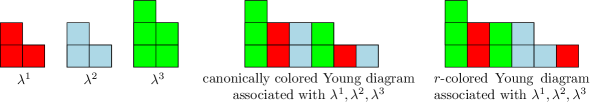
Figure 1. $r$-colored and canonically colored partitions.

When $f_{\lambda}=\tilde{H}_{\lambda}^{(q,t)}$ is the transformed version of the Macdonald polynomial indexed by a partition $\lambda$, the corresponding $q$-partial cumulant $\kappa_{[1..r]}^{(q)}(\bm{u})$ is called the Macdonald cumulant and denoted $\kappa(\lambda^{1},\dots,\lambda^{r})(\bm{x};q,t)$:

(13) $$\kappa(\lambda^{1},\dots,\lambda^{r})(\bm{x};q,t):=\kappa_{[1..r]}^{(q)}(\bm{u}).$$

It was studied in [Doł17, Doł19], where its polynomiality and combinatorial interpretation was obtained, generalizing the celebrated HHL formula (5). Furthermore, it was conjectured in [Doł17] that Macdonald cumulants are Schur-positive:

Conjecture 2.6 ([Doł17]).

Let $\lambda^{1},\dots,\lambda^{r}$ be partitions. Then for any partition $\nu$ the coefficient $[s_{\nu}]\kappa(\lambda^{1},\dots,\lambda^{r})$ in the Schur expansion of the Macdonald cumulant is a polynomial in $q,t$ with nonnegative coefficients.

The first motivation for introducing LLT cumulants is to attack 2.6. Since Macdonald polynomials can be naturally decomposed into LLT polynomials, it is natural to ask whether a similar decomposition occurs for Macdonald cumulants. Moreover, it was proved by Grojnowski and Haiman [GH07] that LLT polynomials are Schur-positive, which gives an alternative proof of the Schur positivity of Macdonald polynomials. Extensive computer simulations performed by the authors using the SageMath computer algebra system [The20] tend us to believe that the result of Grojnowski and Haiman might be a special case of Schur-positivity that holds for the more general class of LLT cumulants. Therefore, we propose the following conjecture:

Conjecture 2.7.

For any $r$-colored tuple of skew shapes $(\bm{\nu},f)$ and for any partition $\lambda$ the coefficient $[s_{\lambda}]\kappa_{\operatorname{LLT}^{\operatorname{cospin}}}(\bm{\nu},f)$ in the Schur expansion of the LLT cumulant is a polynomial in $q$ with nonnegative integer coefficients.

Example.

Let $\bm{\nu}=((2,2)/(1),(2),(1,1))$ be a tuple of three skew shapes. Consider two colorings $f\colon[1..3]\to[1..3]$ and $f^{\prime}\colon[1..3]\to[1..2]$ defined by $f(i)=i$ for $1\leq i\leq 3$ and $f^{\prime}(1)=f^{\prime}(3)=1,f^{\prime}(2)=2$. The corresponding cumulants $\kappa_{\operatorname{LLT}^{\operatorname{cospin}}}(\bm{\nu},f)$ and $\kappa_{\operatorname{LLT}^{\operatorname{cospin}}}(\bm{\nu},f^{\prime})$ are equal to

$$\kappa_{\operatorname{LLT}^{\operatorname{cospin}}}(\bm{\nu},f) =(q-1)^{-2}\bigg{(}\operatorname{LLT}^{\operatorname{cospin}}((2,2)/(1),(2),(1,1))-\operatorname{LLT}^{\operatorname{cospin}}((2,2)/(1))\cdot$$

$$\cdot\operatorname{LLT}^{\operatorname{cospin}}((2),(1,1))-\operatorname{LLT}^{\operatorname{cospin}}((2))\operatorname{LLT}^{\operatorname{cospin}}((2,2)/(1),(1,1))$$

$$-\operatorname{LLT}^{\operatorname{cospin}}((1,1))\operatorname{LLT}^{\operatorname{cospin}}((2,2)/(1),(2))$$

$$+2\operatorname{LLT}^{\operatorname{cospin}}((2,2)/(1))\operatorname{LLT}^{\operatorname{cospin}}((2))\operatorname{LLT}^{\operatorname{cospin}}((1,1))\bigg{)},$$

$$\kappa_{\operatorname{LLT}^{\operatorname{cospin}}}(\bm{\nu},f^{\prime}) =(q-1)^{-1}\bigg{(}\operatorname{LLT}^{\operatorname{cospin}}((2,2)/(1),(2),(1,1))$$

$$-\operatorname{LLT}^{\operatorname{cospin}}((2))\operatorname{LLT}^{\operatorname{cospin}}((2,2)/(1),(1,1))\bigg{)}.$$

Expanding them in the basis of Schur functions we have

$$\kappa_{\operatorname{LLT}^{\operatorname{cospin}}}(\bm{\nu},f) =(q^{2}+2q+2)s_{(2,2,1,1,1)}+(q+2)s_{(2,2,2,1)}$$

$$+(q^{2}+2q+2)s_{(3,1,1,1,1)}+(2q+4)s_{(3,2,1,1)}$$

$$+2s_{(3,2,2)}+s_{(3,3,1)}+(q+2)s_{(4,1,1,1)}+s_{(4,2,1)},$$

$$\kappa_{\operatorname{LLT}^{\operatorname{cospin}}}(\bm{\nu},f^{\prime}) =(q^{3}+q^{2})s_{(2,2,1,1,1)}+(q^{2}+q)s_{(2,2,2,1)}$$

$$+(q^{3}+q^{2})s_{(3,1,1,1,1)}+(2q^{2}+2q)s_{(3,2,1,1)}+(2q+1)s_{(3,2,2)}$$

$$+(q+1)s_{(3,3,1)}+(q^{2}+q)s_{(4,1,1,1)}+(q+1)s_{(4,2,1)}.$$

In the following, we prove that 2.7 implies 2.6. In order to do this, we express Macdonald cumulants as a positive linear combination of LLT cumulants, generalizing the classical decomposition from Theorem 2.2 to cumulants, and we show that Schur-positivity of LLT cumulants can be put into the following hierarchy: Schur-positivity of $\kappa_{\operatorname{LLT}^{\operatorname{cospin}}}(\bm{\nu},f)$ implies Schur-positivity of $\kappa_{\operatorname{LLT}^{\operatorname{Mac}}}(\bm{\nu},f)$, which further implies Schur-positivity of $\kappa_{\operatorname{LLT}}(\bm{\nu},f)$.

Remark 2.8.

In fact, the chain of implications mentioned above is valid only when we restrict $\bm{\nu}$ to be a sequence of ribbon shapes due to the definition of the normalization $\operatorname{LLT}^{\operatorname{Mac}}(\bm{\nu})$ (see (4)). However, Schur-positivity of $\kappa_{\operatorname{LLT}^{\operatorname{cospin}}}(\bm{\nu},f)$ for all $r$-colored tuples of skew-shapes $(\bm{\nu},f)$ implies Schur-positivity of $\kappa_{\operatorname{LLT}}(\bm{\nu},f)$ for all $r$-colored tuples of skew-shapes $(\bm{\nu},f)$, which will be clear from the proof of Theorem 2.10.

2.3.1. Decomposition of Macdonald cumulants

Theorem 2.9.

Let $\lambda^{1},\dots,\lambda^{r}$ be partitions. Then, the following identity holds true:

(14) $$\kappa(\lambda^{1},\dots,\lambda^{r})(\bm{x};q,t)=\sum_{\bm{\nu}}t^{\operatorname{maj}(\bm{\nu})}\kappa_{\operatorname{LLT}^{\operatorname{Mac}}}(\bm{\nu},f_{\operatorname{cc}}),$$

where we sum over all tuples of ribbons whose bottom, far-right cell has content $0$ and such that $|\bm{\nu}_{j}|=(\lambda^{[1..r]})^{\prime}_{j}$ for $1\leq j\leq\ell(\lambda^{[1..r]})$ (i.e. the size of the $j$-th ribbon is equal to the length of the $j$-th column of $\lambda^{[1..r]}$) and $f_{\operatorname{cc}}$ is the canonical coloring associated with $\lambda^{1},\dots,\lambda^{r}$.

Proof.

It is a direct consequence of the interpretation of the Macdonald cumulant as the $q$-partial cumulant of the canonically $r$-colored partition and of Theorem 2.2. Indeed, note that for any subset $B\subset[1..r]$, Theorem 2.2 applied to $\lambda=\lambda^{B}$ gives

$$\tilde{H}_{\lambda^{B}}^{(q,t)}=\sum_{\bm{\nu}}t^{\operatorname{maj}(\bm{\nu})}\operatorname{LLT}^{\operatorname{Mac}}(\bm{\nu}),$$

where we sum over skew-partitions whose $j$-th element is a ribbon of length $(\lambda^{B})^{\prime}_{j}$ whose bottom, far-right cell has content $0$. In particular, for any set-partition $\pi\in\mathcal{P}([1..r])$, one has

$$\prod_{B\in\pi}\tilde{H}_{\lambda^{B}}^{(q,t)}=\sum_{\bm{\nu}}\prod_{B\in\pi}t^{\operatorname{maj}((\bm{\nu},f_{\operatorname{cc}})^{B})}\operatorname{LLT}^{\operatorname{Mac}}((\bm{\nu},f_{\operatorname{cc}})^{B}),$$

where the sum runs over the same set as the summation in (5).

Strictly from the definition (6) of $\operatorname{maj}$, one has $\sum_{B\in\pi}\operatorname{maj}((\bm{\nu},f_{\operatorname{cc}})^{B})=\operatorname{maj}(\bm{\nu})$ for any set-partition $\pi\in\mathcal{P}([1..r])$, and formula (14) follows. ∎

Theorem 2.10.

Suppose that 2.7 holds true. Then, for any $r$-colored tuple of skew shapes $(\bm{\nu},f)$ and for any partition $\nu$, the coefficients

$$[s_{\nu}]\kappa_{\operatorname{LLT}^{\operatorname{Mac}}}(\bm{\nu},f)\in\mathbb{Z}_{\geq 0}[q],\qquad[s_{\nu}]\kappa_{\operatorname{LLT}}(\bm{\nu},f)\in\mathbb{Z}_{\geq 0}[q]$$

are polynomials in $q$ with nonnegative integer coefficients. In particular, 2.6 holds true.

Proof.

Recall the definiton Eq. 10 of LLT cumulants. We will show that there exist graphs $G\subset G^{\prime}$ such that

(15) $$\kappa_{[1..r]}^{(q)}(\bm{u}(\operatorname{LLT})) =\kappa_{[1..r]}^{(q)}(\bm{u}(\operatorname{LLT}^{\operatorname{cospin}})^{G^{\prime}}),$$

(16) $$\kappa_{[1..r]}^{(q)}(\bm{u}(\operatorname{LLT}^{\operatorname{Mac}})) =\kappa_{[1..r]}^{(q)}(\bm{u}(\operatorname{LLT}^{\operatorname{cospin}})^{G}).$$

Then the statements follow directly from Theorem 2.5 and Eq. 14.

Notice that the family of nonnegative integers $(e_{B})_{B\subset V}$ indexed by subsets of the set $V$ is the number of edges in some graph $G=(V,E)$ linking vertices in $B$ if and only if

(17) $$e_{B}\geq\sum_{b\in B}e_{\{b\}}\ \ \ \text{ and }\ \ \ e_{B}=\sum_{\begin{subarray}{c}B^{\prime}\subset B,\\ |B^{\prime}|=2\end{subarray}}e_{B^{\prime}}-(|B|-2)\sum_{b\in B}e_{\{b\}}.$$

Indeed, the inequality corresponds to $e_{B}$ counting all the loops on vertices from $B$, and the equality counts the edges between each pair of vertices from $B$ minus the overcounted loops.

We first prove that there exist graphs $G,G^{\prime}$ such that (15) and (16) hold. To show (15), consider $e_{B}=\min_{T\in\operatorname{SSYT}((\bm{\nu},f)^{B})}\operatorname{inv}(T)=|\operatorname{Inv}(T)\setminus\operatorname{Inv}_{\operatorname{cospin}}(T)|$, which does not depend on the choice of $T\in\operatorname{SSYT}((\bm{\nu},f)^{B})$. Then the conditions in (17) are satisfied since for a pair of boxes $\square\in(\bm{\nu},f)^{\{i\}}$ and $\square^{\prime}\in(\bm{\nu},f)^{\{j\}}$, one has $(\square,\square^{\prime})\in\operatorname{Inv}(T)\setminus\operatorname{Inv}_{\operatorname{cospin}}(T)$ if and only if $(\square,\square^{\prime})\in\operatorname{Inv}(T_{\{i,j\}})\setminus\operatorname{Inv}_{\operatorname{cospin}}(T_{\{i,j\}})$, where $T_{\{i,j\}}$ is a tableau $T$ restricted to $(\bm{\nu},f)^{\{i,j\}}$.

Similarly, for

$$e_{B}=a((\bm{\nu},f)^{B})=\sum_{\square\in\operatorname{Des}((\bm{\nu},f)^{B})}|\{\square^{\prime}:c(\square^{\prime})=c(\square),\tilde{c}(\square^{\prime})>\tilde{c}(\square)\}|,$$

one has

(18) $$\sum_{\square\in\operatorname{Des}((\bm{\nu},f)^{B})}|\{\square^{\prime}\colon c(\square^{\prime})=c(\square),\tilde{c}(\square^{\prime})>\tilde{c}(\square)\}|=\\ \sum_{b\in B}\sum_{\square\in\operatorname{Des}((\bm{\nu},f)^{\{b\}})}\sum_{b^{\prime}\in B}|\{\square^{\prime}\in(\bm{\nu},f)^{\{b^{\prime}\}}\colon c(\square^{\prime})=c(\square),\tilde{c}(\square^{\prime})>\tilde{c}(\square)\}|.$$

Note that for any subset $A\subset B$ and for each pair of boxes $(\square,\square^{\prime})\in(\bm{\nu},f)^{A}$, there is a uniquely associated pair of boxes $(\square,\square^{\prime})\in(\bm{\nu},f)^{B}$ and their contents are identical in $(\bm{\nu},f)^{A}$ and $(\bm{\nu},f)^{B}$, while their shifted contents might be different but the relation $\tilde{c}(\square^{\prime})>\tilde{c}(\square)$ is again the same in both $(\bm{\nu},f)^{A}$ and $(\bm{\nu},f)^{B}$. This observation together with (18) implies that the quantities $e_{B}$ satisfy (17). This proves (16).

Finally, we prove that $G\subset G^{\prime}$, which is equivalent to proving that $a((\bm{\nu},f)^{B})\leq\min_{T\in\operatorname{SSYT}((\bm{\nu},f)^{B})}\operatorname{inv}(T)$. Let $\square\in\operatorname{Des}((\bm{\nu},f)^{B})$ and $\square^{\prime}\in(\bm{\nu},f)^{B}$ be such that $c(\square^{\prime})=c(\square),\tilde{c}(\square^{\prime})>\tilde{c}(\square)$. For any $T\in\operatorname{SSYT}((\bm{\nu},f)^{B})$, we necessarily have $T(\square)>T(\square_{\downarrow})$. Therefore, either $(\square,\square^{\prime})\in\operatorname{Inv}(T)$ or $(\square^{\prime},\square_{\downarrow})\in\operatorname{Inv}(T)$ (or both). Summing over all $\square\in\operatorname{Des}((\bm{\nu},f)^{B})$ and

$$\square^{\prime}\in\{\square^{\prime}\in(\bm{\nu},f)^{B}:c(\square^{\prime})=c(\square),\tilde{c}(\square^{\prime})>\tilde{c}(\square)\},$$

we have that $a((\bm{\nu},f)^{B})\leq\operatorname{inv}(T)$ for any $T\in\operatorname{SSYT}((\bm{\nu},f)^{B})$. Thus, $a((\bm{\nu},f)^{B})\leq\min_{T\in\operatorname{SSYT}((\bm{\nu},f)^{B})}\operatorname{inv}(T)$, which is equivalent to the fact that $G\subset G^{\prime}$. This implies that $[s_{\nu}]\kappa_{\operatorname{LLT}^{\operatorname{Mac}}}(\bm{\nu},f)$ and $[s_{\nu}]\kappa_{\operatorname{LLT}}(\bm{\nu},f)$ are indeed polynomials in $q$, which finishes the proof. ∎

3. Graph colorings

In the following, we interpret LLT polynomials as the generating functions of colorings of certain directed graphs. This viewpoint provides a natural graph-theoretic interpretation of LLT cumulants as well as various positivity properties generalizing some recent results [AS22, Doł19].

3.1. LLT graphs and cumulants of $r$-colored LLT graphs

Definition 3.1.

We call $G$ an LLT graph if it is a finite directed graph with three types of edges, visually depicted as $\rightarrow$, $\twoheadrightarrow$, and $\Rightarrow$, which we call edges of type I, of type II, and double edges, respectively. Denote the corresponding sets of edges by $E_{1}(G)$, $E_{2}(G)$, and $E_{d}(G)$. Additionally, write $\mathscr{G}$ for the $\mathbb{Z}[q]$-module spanned by LLT graphs and $\mathscr{G}_{1}<\mathscr{G}$ for the submodule generated by LLT graphs with only edges of type II ($E_{1}(G)=E_{d}(G)=\emptyset$).

Let $\operatorname{QSym}$ denote the ring of quasi-symmetric functions over $\mathbb{Z}[q]$. We recall that a quasisymmetric function $f$ is a power series in variables $x_{1},x_{2},\dots$ of a bounded degree such that for any sequence of positive integers $(\alpha_{1},\dots,\alpha_{n})$ the coefficients of the monomial $[x_{i_{1}}^{\alpha_{1}}\cdots x_{i_{n}}^{\alpha_{n}}]f$ in $f$ is the same for all possible choices of indices $i_{1}<\dots<i_{n}$ (see [Ges84] for more details on $\operatorname{QSym}$). With an LLT graph $G$ we associate its LLT polynomial:

(19) $$\operatorname{LLT}(G):=\sum\limits_{f:V(G)\rightarrow\mathbb{N}}\left(\prod\limits_{(u,v)\in E(G)}\varphi_{f}(u,v)\right)\cdot\left(\prod\limits_{v\in V(G)}x_{f(v)}\right),$$

with

(20) $$\varphi_{f}(u,v)=\begin{cases}[f(u)>f(v)]&\text{for }(u,v)\in E_{1}(G);\\ [f(u)\geq f(v)]&\text{for }(u,v)\in E_{2}(G);\\ q[f(u)>f(v)]+[f(u)\leq f(v)]&\text{for }(u,v)\in E_{d}(G),\end{cases}$$

where $[A]$ is the characteristic function of condition $A$, i.e., is equal to $1$ if $A$ is true and $0$ otherwise.

There is an obvious way to associate an LLT graph $G_{\bm{\nu}}$ to a sequence of skew shapes $\bm{\nu}$ such that $\operatorname{LLT}(G_{\bm{\nu}})=\operatorname{LLT}(\bm{\nu})$. To be precise, vertices correspond to cells, edges of type I go from a cell $\square$ to $\square_{\downarrow}$, edges of type II go from a cell $\square$ to $\square_{\leftarrow}$, and double edges connect cells that correspond to inversions (see Fig. 2).

Figure 2. The LLT graph corresponding to ((3,2)/(1), (1,1)).

Let $G$ be an LLT graph and let $\vec{e_{i}}\in E_{i}(G)$ for $i\in\{1,d\}$. Define the local transformation

$$\pi_{\vec{e_{i}}}(G)=\begin{cases}G\setminus\{\vec{e_{1}}\}-G_{\vec{e_{1}}\to\cev{e_{2}}}&\text{ for }i=1,\\ qG\setminus\{\vec{e_{d}}\}+(1-q)G_{\vec{e_{d}}\to\cev{e_{2}}}&\text{ for }i=d,\end{cases}$$

where $\vec{e_{i}}\to\cev{e_{j}}$ ($\vec{e_{i}}\to\vec{e_{j}}$, respectively) denotes replacing the directed edge $\vec{e_{i}}$ of type $i$ by the edge of type $j$ with the opposite (the same, respectively) direction.

Example.

We have

$$\pi_{(1,2)}\left(\vbox{\hbox{ \leavevmode\hbox to46.49pt{\vbox to46.65pt{\text{[drawing]}}}}}\right)=\vbox{\hbox{ \leavevmode\hbox to46.49pt{\vbox to46.65pt{\text{[drawing]}}}}}-\vbox{\hbox{ \leavevmode\hbox to46.49pt{\vbox to46.65pt{\text{[drawing]}}}}}, 1 2 3 1 2 3 1 2 3 1 2 3 1 2 3 1 2 3$$

$$\pi_{(1,3)}\left(\vbox{\hbox{ \leavevmode\hbox to46.49pt{\vbox to46.65pt{\text{[drawing]}}}}}\right)=q\vbox{\hbox{ \leavevmode\hbox to46.49pt{\vbox to46.65pt{\text{[drawing]}}}}}+(1-q)\vbox{\hbox{ \leavevmode\hbox to46.49pt{\vbox to46.65pt{\text{[drawing]}}}}}. 1 2 3 1 2 3 1 2 3 1 2 3 1 2 3 1 2 3$$

We define

$$\pi(G):=\bigg{(}\prod_{\vec{e}\in E_{1}(G)\cup E_{d}(G)}\pi_{\vec{e}}\bigg{)}(G)$$

as the concatenation of local transformations over all edges of type I and double edges (these transformations are commutative so their order does not matter and this concatenation is well-defined). Note that local transformations kill all edges of type I and $d$ and thus, the map $\pi\colon\mathscr{G}\to\mathscr{G}_{1}$ is well-defined. In fact, we claim that the map $\operatorname{LLT}\colon\mathscr{G}\to\operatorname{QSym}$ is a well-defined surjective homomorphism such that $\operatorname{LLT}(G)=\operatorname{LLT}\circ\pi(G)$ for every LLT graph.

Lemma 3.2.

For $\mathscr{G}$ and $\mathscr{G}_{1}$ as in Definition 3.1, the following diagram is commutative:

Proof.

Let $G$ be an LLT graph. It was proved by Féray [F1́5] that $\operatorname{LLT}\colon\mathscr{G}_{1}\to\operatorname{QSym}$ is a well-defined surjective homomorphism. Moreover, it is straightforward from the definition of the map $\operatorname{LLT}$ that it is invariant under the local transformations, i.e., for every $\vec{e}\in E_{1}(G)\cup E_{d}(G)$, one has $\operatorname{LLT}(\pi_{\vec{e}}(G))=\operatorname{LLT}(G)$. Thus, $\operatorname{LLT}(G)=\operatorname{LLT}(\pi(G))$, which finishes the proof. ∎

Remark 3.3.

Let $\widehat{\mathscr{G}}_{1}<\mathscr{G}_{1}$ be a submodule of $\mathscr{G}_{1}$ spanned by acyclic graphs. The main result of Féray [F1́5] is an explicit description of the kernel of the map $\operatorname{LLT}\colon\widehat{\mathscr{G}}_{1}\to\operatorname{QSym}$ by using the cyclic inclusion-exclusion principle. This description together with Lemma 3.2 can be a priori used to describe the kernel of the morphism $\operatorname{LLT}\colon\mathscr{G}\to\operatorname{QSym}$, thus to understand all the relations between LLT graphs under the $\operatorname{LLT}$ morphism. Additionally, $\mathscr{G}$ seems to carry a natural Hopf algebra structure. Studying various relations between LLT polynomials is a very active topic recently and it proved to be useful in understanding the combinatorial structure of LLT polynomials [Lee21, HNY20, AN21, AS22, Tom21]. We believe that further studies in the direction of understanding the algebraic structure of the pair $(\mathscr{G},\operatorname{LLT})$ might bring better understanding of the combinatorial structure of LLT polynomials, and we leave this problem for future research.

As a consequence of Lemma 3.2 and its proof, we obtain two identities expressing the LLT polynomial of a given LLT graph $G$ in terms of two important LLT graphs, which do not have any double edges. For any subset $E\subset E_{d}(G)$, we define $G^{E}$ and $\tilde{G}^{E}$ as follows:

• $V(\tilde{G}^{E})=V(G^{E})=V(G)$,

• $E_{d}(\tilde{G}^{E})=E_{d}(G^{E})=\emptyset$,

• $E_{1}(\tilde{G}^{E})=E_{1}(G^{E})=E_{1}(G)\cup E$,

• $E_{2}(\tilde{G}^{E})=E_{2}(G)\cup\{(u,v)\mid(v,u)\in E_{d}\setminus E\}$, and $E_{2}(G^{E})=E_{2}(G)$.

Example.

For

$$G=\vbox{\hbox{ \leavevmode\hbox to93.25pt{\vbox to47.72pt{\text{[drawing]}}}}}$$

and $E\subset E_{d}(G)$ equal to the set of the red edges above, we have

$$G^{E}=\vbox{\hbox{ \leavevmode\hbox to91.85pt{\vbox to46.32pt{\text{[drawing]}}}}},\hskip 71.13188pt\tilde{G}^{E}=\vbox{\hbox{ \leavevmode\hbox to91.85pt{\vbox to46.32pt{\text{[drawing]}}}}}.$$

Corollary 3.4.

For any LLT graph $G$, we have

$$\operatorname{LLT}(G)=\sum_{E\subseteq E_{d}(G)}q^{|E|}\operatorname{LLT}(\tilde{G}^{E})=\sum_{E\subseteq E_{d}(G)}(q-1)^{|E|}\operatorname{LLT}(G^{E}).$$

Proof.

Note that

$$\bigg{(}\prod_{\vec{e}\in E_{d}(G)}\pi^{\prime}_{\vec{e}}\bigg{)}(G)=\sum_{E\subseteq E_{d}(G)}q^{|E|}\tilde{G}^{E},\ \ \bigg{(}\prod_{\vec{e}\in E_{d}(G)}\pi^{\prime\prime}_{\vec{e}}\bigg{)}(G)=\sum_{E\subseteq E_{d}(G)}(q-1)^{|E|}G^{E},$$

where $\pi^{\prime}_{\vec{e_{d}}}(G)=G_{\vec{e_{d}}\to\cev{e_{2}}}+qG_{\vec{e_{d}}\to\vec{e_{1}}}$ and $\pi^{\prime\prime}_{\vec{e_{d}}}(G)=G\setminus\{\vec{e_{d}}\}+(q-1)G_{\vec{e_{d}}\to\vec{e_{1}}}$ for $e_{d}\in E_{d}(G)$. Moreover, $\operatorname{LLT}(G)=\operatorname{LLT}(\pi^{\prime}_{\vec{e_{d}}}(G))$ follows from the definition, and $\operatorname{LLT}(G)=\operatorname{LLT}(\pi^{\prime\prime}_{\vec{e_{d}}}(G))$ follows from

$$\operatorname{LLT}(G)=\operatorname{LLT}(G_{\vec{e_{d}}\to\cev{e_{2}}})+q\operatorname{LLT}(G_{\vec{e_{d}}\to\vec{e_{1}}})=\operatorname{LLT}(G\setminus\{\vec{e_{d}}\})+(q-1)\operatorname{LLT}(G_{\vec{e_{d}}\to\vec{e_{1}}})$$

since we have that $\operatorname{LLT}(G_{\vec{e_{d}}\to\cev{e_{2}}})=\operatorname{LLT}(G\setminus\{\vec{e_{d}}\})-\operatorname{LLT}(G_{\vec{e_{d}}\to\vec{e_{1}}})$. ∎

The definition of LLT cumulants of $r$-colored tuples of skew-shapes generalizes naturally to the definition of LLT cumulants of $r$-colored LLT graphs.

Definition 3.5.

We say that $(G,f)$ is an $r$-colored LLT graph if $G$ is an LLT graph and $f\in V(G)\to[1..r]$ is a surjective coloring of vertices of $G$ such that both endpoints of edges in $E_{1}(G)\cup E_{2}(G)$ have the same color. For any subset $B\subset[1..r]$, we define the vertex set $V_{B}:=\{v\in V(G)\colon f(v)\in B\}$ and for any subset $V^{\prime}\subset V(G)$, we define $G|_{V}$ as the subgraph of $G$ obtained by restricting its set of vertices to $V^{\prime}$. Then, we define the LLT cumulant of an $r$-colored LLT graph $(G,f)$ as the $q$-partial cumulant $\kappa^{(q)}_{[1..r]}(\bm{u})$ for the family defined by

$$u_{B}:=\operatorname{LLT}(G|_{V_{B}}).$$

Observe that the first equation in Corollary 3.4 is, in fact, a special case of a more general formula:

Corollary 3.6.

For any set-partition $\pi\in\mathcal{P}([1..r])$, one has

(21) $$\prod_{B\in\pi}\operatorname{LLT}(G|_{V_{B}})=\sum_{E\subseteq E_{d}(G)}\operatorname{LLT}(\tilde{G}^{E})\prod_{B\in\pi}q^{|E_{B}|},$$

where $E_{B}\subset E$ is the subset of edges with both endpoints in $B$.

Proof.

Formula (21) is proved similarly to Corollary 3.4, so we only sketch the proof. Let $G_{\pi}:=\bigoplus_{B\in\pi}G|_{V_{B}}$, where $G_{1}\oplus G_{2}$ is a disjoint union of the LLT graphs $G_{1}$ and $G_{2}$. Then $\prod_{B\in\pi}\operatorname{LLT}(G|_{V_{B}})=\operatorname{LLT}(G_{\pi})$. Note that $G_{\pi}$ is obtained from $G$ by removing all the double edges connecting vertices with colors lying in different blocks of $\pi$. Consider two local transformations: $\pi^{\prime}_{\vec{e}}(G_{\pi})$ for $\vec{e}\in E_{d}(G_{\pi})$ and $\pi^{\prime\prime\prime}_{\vec{e}}(G_{\pi}):=(G_{\pi})_{\vec{e}\to\vec{e_{1}}}+(G_{\pi})_{\vec{e}\to\cev{e_{2}}}$ for any orientation $\vec{e}$ of $e\notin E(G_{\pi})$. Notice that

$$\bigg{(}\prod_{\vec{e}\in E_{d}(G_{\pi})\atop\vec{\tilde{e}}\in E_{d}(G)\setminus E_{d}(G_{\pi})}\pi^{\prime}_{\vec{e}}\pi^{\prime\prime\prime}_{\vec{\tilde{e}}}\bigg{)}(G_{\pi})=\sum_{E\subseteq E_{d}(G)}\tilde{G}^{E}\prod_{B\in\pi}q^{|E_{B}|}.$$

Finally, recall that $\operatorname{LLT}$ is invariant under taking the local transformation $\pi^{\prime}_{\vec{e}}$ and notice that $\operatorname{LLT}(G)=\operatorname{LLT}(\pi^{\prime\prime\prime}_{\vec{e}}(G))$ for any orientation $\vec{e}$ of $e\notin E(G)$. This finishes the proof. ∎

In the following, we prove that the LLT cumulant of the $r$-colored LLT graph $(G,f)$ can be naturally expressed as a sum of LLT polynomials of so-called $f$-connected graphs.

Definition 3.7.

Let $(G,f)$ be an $r$-colored LLT graph. We say that it is $f$-connected if the graph $G_{f}$ obtained from $G$ by identifying vertices of the same color is connected. In other words, the graph $G$ is $f$-connected if for every pair $i,j\in[1..r]$, there exists $i=i_{0}\neq i_{1}\cdots\neq i_{k}=j\in[1..r]$ and vertices $v_{0},\dots,v_{k}\in V(G)$ colored by $i_{0},\dots,i_{k}$ respectively such that $v_{i-1}$ is connected to $v_{i}$ for every $1\leq i\leq k$.

Note that when $f$ is a bijection then the graph $G$ is $f$-connected if and only if $G$ is connected, and if $f$ is a $1$-coloring then the condition of being $f$-connected is empty (it is always satisfied). We have the following combinatorial interpretation of an LLT cumulant of an $r$-colored LLT graph $(G,f)$.

Theorem 3.8.

Let $(G,f)$ be an $r$-colored LLT graph and denote $E_{d}=E_{d}(G)$. Then:

(22) $$\kappa_{\operatorname{LLT}}(G,f)(q+1)=\sum\limits_{\begin{subarray}{c}E\subseteq E_{d}\\ G^{E}\text{ $f$-connected}\end{subarray}}q^{|E|-r+1}\operatorname{LLT}(G^{E})(q+1).$$

Theorem 3.8 essentially shows the structure behind the, a priori, algebraic definition of a cumulant: it kills all $f$-disconnected summands in the expansion and preserves the $f$-connected ones. Furthermore, we note that we formulate the statement with the polynomials evaluated at $q+1$ to highlight the $\operatorname{LLT}$-positivity of the cumulant after the shift $q\longmapsto q+1$: an operation that is also relevant in the context of the $e$-positivity phenomenon (see Section 3.2.4).

Proof of Theorem 3.8.

We have

$$\kappa_{\operatorname{LLT}}(G,f)(q+1): =q^{1-r}\sum_{\pi\in\mathcal{P}([1..r])}(-1)^{|\pi|-1}(|\pi|-1)!\prod_{B\in\pi}\operatorname{LLT}(G|_{V_{B}})$$

$$=q^{1-r}\sum_{\pi\in\mathcal{P}([1..r])}(-1)^{|\pi|-1}(|\pi|-1)!\operatorname{LLT}\left(G_{\pi}\right),$$

where we recall that $G_{\pi}:=\bigoplus_{B\in\pi}G|_{V_{B}}$.

By Corollary 3.4, for each $B\in\mathcal{P}([1..r])$, we get

(23) $$\operatorname{LLT}\left(G_{\pi}\right)(q+1)=\sum_{E\subseteq E_{d}(G_{\pi})}q^{|E|}\operatorname{LLT}(G_{\pi}^{E})(q+1)$$

so that

(24) $$\kappa_{\operatorname{LLT}}(G,f)(q+1)=q^{1-r}\sum_{\pi\in\mathcal{P}([1..r])}(-1)^{|\pi|-1}(|\pi|-1)!\sum_{E\subseteq E_{d}(G_{\pi})}q^{|E|}\operatorname{LLT}(G_{\pi}^{E})(q+1).$$

Now consider an LLT graph $G^{\prime}=G_{\sigma}^{E}$ for some $\sigma\in\mathcal{P}([1..r])$ and $E\subseteq E_{d}(G_{\sigma})$. For a fixed $G^{\prime}$ of this form, pick $\sigma$ to be minimal, i.e.  pick $\sigma$ such that for every block $B\in\sigma$, the graph $G^{\prime}|_{V_{B}}$ is $f$-connected. Note that $G^{\prime}$ is $f$-connected if and only if $\sigma=\{[1..r]\}$. We compute the contribution of the graph $G^{\prime}$ to the RHS of the formula (24).

Note that $G^{\prime}$ appears in a summand corresponding to a partition $\pi$ if and only if for every $B\in\sigma$, there exists $C\in\pi$ such that $B\subseteq C$. This is known as the containment relation $\sigma\leq\pi$ on the set of set-partitions. Therefore, we have

$$[\operatorname{LLT}(G^{\prime})(q+1)]\kappa_{\operatorname{LLT}}(G,f) =q^{|E|-r+1}\sum_{\sigma\leq\pi}(-1)^{|\pi|-1}(|\pi|-1)!=q^{|E|-r+1}\delta_{\sigma,\{[1..r]\}}.$$

The last equality comes from the well-known fact that $(-1)^{|\pi|-1}(|\pi|-1)!$ is equal to the Möbius function $\mu(\pi,\{[1..r]\})$ on the poset of set-partitions $(\mathcal{P}([1..r]),\leq)$ and the sum of the Möbius function $\mu(\pi,\{[1..r]\})$ over the interval $\pi\in[\sigma,\{[1..r]\}]$ is non-zero (and equal to $1$) only if $\sigma=\{[1..r]\}$ (see, e.g., [Wei35]). This finishes the proof as $\sigma=\{[1..r]\}$ if and only if $G^{\prime}$ is $f$-connected. ∎

3.2. Various positivity results

The purpose of this section is to derive various combinatorial formulae for an LLT cumulant of an $r$-colored LLT graph and proving certain positivity results. We start by a quick review on $G$-inversion polynomials and their different interpretations.

3.2.1. $G$-inversion polynomials and Tutte polynomials

Let $G$ be a multigraph (with possible multiedges and multiloops, as previously) on the set of vertices $[1..r]$. We say that $T$ is a spanning tree of $G$ if it is a subgraph of $G$ with the same set of vertices $[1..r]$ and it is a tree (it is connected and has no cycles). A pair $(i,j)$ is called an inversion of a spanning tree $T$ of $G$ if $i,j\neq 1$ and if $i$ is an ancestor of $j$ and $i>j$. An inversion $(i,j)$ is a $\kappa$-inversion if, additionally, $j$ is adjacent to the parent of $i$ in $G$. A $G$-inversion polynomial is a generating function of spanning trees of $G$ counted with respect to the number of $\kappa$-inversions.

Let $\tilde{G}$ be a graph obtained from $G$ by replacing all multiple edges by single ones. We recall that for any subset $B\subset V$ we denote the number of edges linking vertices in $B$ by $e_{B}$. The $G$-inversion polynomial is given by

(25) $$\mathcal{I}_{G}(q)=q^{\text{number of loops in }G}\sum_{T\subset\tilde{G}}q^{\kappa(T)}\prod_{\{i,j\}\in T}[e_{\{i,j\}}(G)]_{q},$$

where the sum runs over all spanning trees of $\tilde{G}$,

(26) $$\kappa(T)=\sum_{\{i,j\}-\kappa-\text{inversion in }T}e_{\{\text{parent}(i),j\}}(G),$$

and we use the standard notation $[n]_{q}:=\frac{q^{n}-1}{q-1}=1+q+\cdots+q^{n-1}$. As we already mentioned in the introduction, $\mathcal{I}_{G}(q)=\operatorname{Tutte}(1,q)$, where $\operatorname{Tutte}(x,y)$ is the Tutte polynomial of $G$ (a classical graph invariant introduced by Tutte in [Tut54]):

(27) $$\operatorname{Tutte}_{G}(x,y)=\sum_{H\subset G}(x-1)^{c(H)-1}\ (y-1)^{|E(H)|-|V|+c(H)}.$$

The summation index above runs over all (possibly disconnected) subgraphs of $G$, $c(H)$ denotes the number of connected components of $H$, and $E(H)$ is the set of edges of $H$. In fact, we have the following lemma, which is essentially due to Gessel [Ges95] and Josuat-Vergès [JV13] (see also [Doł19] for treating both frameworks in the setting of multigraphs).

Lemma 3.9.

Let $G$ be a multigraph with the vertex set $V=[1..r]$ and let $\bm{u}$ be a family indexed by subsets of $[1..r]$ defined as $u_{B}:=q^{e_{B}}$ for every $B\subset[1..r]$. Then we have the following equalities between the generating series:

(28) $$\mathcal{I}_{G}(q)=\operatorname{Tutte}_{G}(1,q)=\kappa^{(q)}(\bm{u}).$$

3.2.2. Monomial positivity

Here, we prove the following theorem implying positivity of LLT cumulants for arbitrary $r$-colored LLT graphs in the quasi-symmetric monomial basis (this is a refinement of the main result from [Doł19]):

Theorem 3.10.

Let $(G,f)$ be an $r$-colored LLT graph and denote $E_{d}=E_{d}(G)$. Then:

(29) $$\kappa_{\operatorname{LLT}}(G,f)(q)=\sum\limits_{\begin{subarray}{c}E\subseteq E_{d}\\ \hat{G}^{E}\text{ $f$-connected}\end{subarray}}\mathcal{I}_{(\hat{G}^{E})_{f}}(q)\operatorname{LLT}(\tilde{G}^{E})(q),$$

where $\hat{G}^{E}$ is obtained from $\tilde{G}^{E}$ by removing all the edges of type II (i.e. $E(\hat{G}^{E})=E(\tilde{G}^{E})\setminus E_{2}(\tilde{G}^{E})$).

Proof.

Let $\hat{G}^{E}$ be a graph obtained from $\tilde{G}^{E}$ by removing all the edges of type II and we recall that $(\hat{G}^{E})_{f}$ is a graph obtained from $\hat{G}^{E}$ by identifying vertices of the same color, i.e. $v\sim w$ if $f(v)=f(w)$. Note that the vertex set of $(\hat{G}^{E})_{f}$ is equal to $[1..r]$ and $|E_{B}|$ in the previous formula is equal to the number of edges of $(\hat{G}^{E})_{f}$ with both endpoints belonging to $B$ (that we denote by $e_{B}$ to be consistent with the previous notation). Therefore, following (21), we end up with the formula

$$\kappa_{\operatorname{LLT}}(G,f) =(q-1)^{1-r}\sum_{E\subseteq E_{d}(G)}\operatorname{LLT}(\tilde{G}^{E})\bigg{(}\sum_{\pi\in\mathcal{P}([1..r])}(-1)^{|\pi|-1}(|\pi|-1)!\prod_{B\in\pi}q^{|E_{B}|}\bigg{)}$$

$$=\sum_{E\subseteq E_{d}(G)}\kappa^{(q)}_{[1..r]}(\bm{u})\operatorname{LLT}(\tilde{G}^{E}),$$

where $u_{B}:=q^{e_{B}}$. This can be rewritten as

$$\sum_{E\subseteq E_{d}(G)}\mathcal{I}_{(\hat{G}^{E})_{f}}(q)\operatorname{LLT}(\tilde{G}^{E})(q)$$

thanks to Lemma 3.9. Finally, $\mathcal{I}_{(\hat{G}^{E})_{f}}(q)=0$ whenever $(\hat{G}^{E})_{f}$ is not connected (because disconnected graphs have no spanning trees), which is the very definition of being $f$-connected for $\hat{G}^{E}$. This finishes the proof. ∎

3.2.3. Fundamental quasisymmetric functions and 2.7 for hooks

For any non-negative integer $n$ and a subset $A\subset[n-1]$, we define the fundamental quasisymmetric function $F_{n,A}(\bm{x})$ to be the expression

$$F_{n,A}(\bm{x}):=\sum_{\begin{subarray}{c}i_{1}\leq\dots\leq i_{n}\\ j\in A\Longrightarrow i_{j}<i_{j+1}\end{subarray}}x_{i_{1}}\dots x_{i_{n}}.$$

We say that a tableau $T\in\operatorname{SSYT}(\bm{\nu})$ of a sequence $\bm{\nu}$ with $|\bm{\nu}|=n$ is standard if $T:\bm{\nu}\rightarrow[n]$ is a bijection, and denote that fact by $T\in\operatorname{SYT}(\bm{\nu})$. We also define the set of descents $\operatorname{Des}(T)$ of $T$ (note that this is not the same as the set of descents of a tuple of skew shapes $\bm{\nu}$, which appeared in the definition of Macdonald polynomials) as the set of $i\in[1..n]$ such that $\tilde{c}(T^{-1}(i+1))<\tilde{c}(T^{-1}(i))$.

In [HHL05a], Haglund, Haiman and Loehr implicitly proved the following formula for the expansion of LLT polynomials in the fundamental quasisymmetric functions.

Theorem 3.11 ([HHL05a]).

For a sequence of skew shapes $\bm{\nu}$ with $|\bm{\nu}|=n$, we have

(30) $$\operatorname{LLT}(\bm{\nu})=\sum\limits_{T\in\operatorname{SYT}(\bm{\nu})}q^{\operatorname{inv}(T)}F_{n,\operatorname{Des}(T)}(\bm{x}).$$

What is more, we can obtain a similar result in our language and notation.

Corollary 3.12.

For any $r$-colored tuple $(\bm{\nu},f)$ of size $n$ and for any set partition $\pi\in\mathcal{P}([1..r])$, we have

(31) $$\prod_{B\in\pi}\operatorname{LLT}((\bm{\nu},f)^{B})=\sum\limits_{T\in\operatorname{SYT}(\bm{\nu})}q^{\operatorname{inv}_{\pi}(T)}F_{n,\operatorname{Des}(T)}(\bm{x}),$$

where $\operatorname{inv}_{\pi}(T)$ denotes the number of inversions in $T$ with both boxes in the same block of $\pi$.

Proof.

The result is a straightforward application of the arguments used in  [HHL05a]. ∎

Applying the same proof as in Theorem 3.10 to (31), we obtain the following result (see also [Doł19, Section 5] for an analogous argument applied to Macdonald cumulants):

Theorem 3.13.

Let $(\bm{\nu},f)$ be an $r$-colored sequence of skew shapes of size $n$. Then:

(32) $$\kappa_{\operatorname{LLT}}(\bm{\nu},f)(q)=\sum\limits_{T\in\operatorname{SYT}(\bm{\nu})}\sum\mathcal{I}_{(\widehat{G_{\bm{\nu}}}^{E^{T}})_{f}}(q)F_{n,\operatorname{Des}(T)}(\bm{x}),$$

where the second sum runs over all subsets $E^{T}\subseteq E_{d}(G_{\bm{\nu}})$ for which $\widehat{G_{\bm{\nu}}}^{E^{T}}$ is $f$-connected and $T(i)>T(j)$ whenever $(i,j)\in E(\widehat{G_{\bm{\nu}}}^{E^{T}})$.

In [Doł19], we were able to find an explicit formula for the coefficients of Schur symmetric functions indexed by hooks, i.e.,  partitions of the form $(k,1^{n-k})$, in Macdonald cumulants, thanks to the arguments from [HHL05a]. Here, we will use a very nice theorem of Egge, Loehr and Warrington [ELW10] which gives a combinatorial description of Schur coefficients of any symmetric function when given an expansion in fundamental quasisymmetric functions.

Theorem 3.14 ([ELW10]).

Suppose that

$$\sum\limits_{\lambda\vdash n}c_{\lambda}s_{\lambda}=\sum\limits_{\alpha\models n}d_{\alpha}F_{n,A(\alpha)},$$

where $A(\alpha)=(\alpha_{1},\alpha_{1}+\alpha_{2},\dots,\sum_{i=1}^{\ell(\alpha)-1}\alpha_{i})$. Then we have $c_{(k,1^{n-k})}=d_{(k,1^{n-k})}$ for all $1\leq k\leq n$.

The original result from [ELW10] gives a description of the coefficients $c_{\lambda}$ for a general $\lambda\vdash n$. However, since we only need the case in the statement (i.e., when $\lambda$ is a hook), we refer interested readers to [ELW10] for the general version, which is slightly more complicated.

The following theorem is an immediate corollary of Theorem 3.13 and Theorem 3.14:

Theorem 3.15.

Let $(\bm{\nu},f)$ be an $r$-colored sequence of skew shapes of size $n$. Then for any $1\leq k\leq n$

$$[s_{(k,1^{n-k})}]\kappa_{\operatorname{LLT}}(\bm{\lambda})=\sum\limits_{\begin{subarray}{c}T\in\operatorname{SYT}(\bm{\lambda})\\ \operatorname{Des}(T)=\{k,k+1,\dots,n-1\}\end{subarray}}\sum\mathcal{I}_{(\widehat{G_{\bm{\nu}}}^{E^{T}})_{f}}(q),$$

where the second sum runs over all subsets $E^{T}\subseteq E_{d}(G_{\bm{\nu}})$ for which $\widehat{G_{\bm{\nu}}}^{E^{T}}$ is $f$-connected and $T(i)>T(j)$ whenever $(i,j)\in E(\widehat{G_{\bm{\nu}}}^{E^{T}})$.

3.2.4. e-positivity

Let $(e_{\lambda})$ be the basis of elementary symmetric functions, i.e.  $e_{\lambda}:=\prod_{i=1}^{\ell(\lambda)}e_{\lambda_{i}}$, where $e_{i}:=\sum_{j_{1}<\cdots<j_{i}}x_{j_{1}}\cdots x_{j_{i}}$ is the $i$-th elementary symmetric function. $e$-positivity of a given symmetric function $f$ is a stronger property than Schur-positivity and it suggests a specific interpretation of the function $f$ in terms of the representation theory of the symmetric group, and in algebro-geometric context. This observation recently generated a lot of research in studying $e$-positive symmetric functions, and after a series of conjectures [Ber17, AP18, GHQR19], it was clear that $e$-positivity of a big class of symmetric functions would be a consequence of $e$-positivity for vertical-strip LLT polynomials after the shift $q\to q+1$, i.e. for $\operatorname{LLT}(\bm{\nu})(q+1)$ where $(\bm{\nu})_{i}=(1^{n_{i}+k_{i}})/(1^{k_{i}})$ for each $1\leq i\leq\ell(\bm{\nu})$ and some nonnegative integers $n_{i},k_{i}$. An explicit combinatorial formula for the coefficients of vertical-strip LLT polynomials in the basis of elementary functions was independently conjectured in [GHQR19, Ale21] and shortly afterwards the positivity (without proving the combinatorial interpretation) was proved in [D’A20] and subsequently [AS22] finalized the picture by proving the combinatorial interpretation. In the following, we reformulate this combinatorial interpretation in our current framework.

Let $\bm{\nu}$ be a tuple of vertical-strips and let $G=G_{\bm{\nu}}$ be the associated LLT-graph. We recall that a vertex $v\in V(G)$ is associated with a box $\square(v)\in\bm{\nu}$ and the vertices are naturally labeled by the shifted contents of the corresponding boxes $\tilde{c}(v):=\tilde{c}(\square(v))$. Fix $E\subset E_{d}(G)$ and define $G^{\prime}=G^{E}$. Since $G^{\prime}$ is a directed graph (note that the condition that $\bm{\nu}$ is a tuple of vertical strips implies that $G^{\prime}$ has only edges of type I), some of the vertices of $G^{\prime}$ have only outgoing edges – such vertices are called sources. We define the following equivalence relation on the set of vertices $V(G^{\prime})$: the vertices $v\sim w$ are in the same equivalence class if the source $\theta(v)$ with the smallest label from which there exists a directed path to $v$ is the same as the source $\theta(w)$ with the smallest label from which there exists a directed path to $w$. The partition $\lambda(G^{\prime})$ is defined as the partition whose parts are sizes of the equivalence classes in this relation. See Fig. 3 for an example.

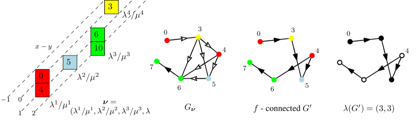
Figure 3. A tuple $\bm{\nu}$ of vertical strips and the associated LLT graph $G_{\bm{\nu}}$. The labels of vertices are the shifted contents of the corresponding boxes. Graph $G^{\prime}=G^{E}$ for $E=\{(0,3),(3,5),(4,5),(4,6)\}$ is $f$-connected, where $f(i)=i$. In the last picture, the displayed labels are the labels of the sources of $G^{\prime}$ and the corresponding two equivalence classes $\{0,3,5\}$ and $\{4,6,7\}$ are depicted by the whole and the empty vertices, respectively.

Theorem 3.16.

[AS22] Let $\bm{\nu}$ be a tuple of vertical-strips and let $G=G_{\bm{\nu}}$ be the associated LLT-graph. Then

(33) $$\operatorname{LLT}(\bm{\nu})(q+1)=\sum_{E\subseteq E_{d}(G)}q^{|E|}e_{\lambda(G^{E})}.$$

In the following, we show that the vertical-strip LLT cumulants preserve $e$-positivity, which refines Theorem 3.16, but, most importantly, shows that $e$-positivity of vertical-strip LLT polynomials naturally decomposes into $f$-connected components, each corresponding to the vertical-strip LLT cumulant. In other terms, heuristically, the e-positivity of vertical-strip LLT polynomials is “built” from e-positivity of LLT cumulants, which naturally decompose LLT polynomials from the graph-coloring point of view.

Theorem 3.17.

Let $(\bm{\nu},f)$ be an $r$-colored tuple of vertical-strips and let $G=G_{\bm{\nu}}$ be the associated LLT-graph. Then

(34) $$\kappa_{\operatorname{LLT}}(\bm{\nu},f)(q+1)=\sum\limits_{\begin{subarray}{c}E\subseteq E_{d}\\ G^{E}\text{ $f$-connected}\end{subarray}}q^{|E|+1-r}e_{\lambda(G^{E})}.$$

Proof.

We recall that the $q$-partial cumulant of the family $(\bm{u})$ is defined by the formula (2.3). One can invert this formula in order to express $u_{I}$ in terms of the $q$-partial cumulants:

$$u_{I}=\sum_{\pi\in\mathcal{P}(I)}(q-1)^{|I|-|\pi|}\prod_{B\in\pi}\kappa_{B}^{(q)}(\bm{u}).$$

Applying this to our setting, we obtain that for any $r\geq 1$ and for any $r$-colored tuple $(\bm{\nu},f)$, one has

$$\operatorname{LLT}(\bm{\nu})(q+1)=\sum_{\pi\in\mathcal{P}([1..r])}q^{r-|\pi|}\prod_{B\in\pi}\kappa_{\operatorname{LLT}}((\bm{\nu},f)^{B},f|_{B})(q+1),$$

where $f|_{B}$ is the $|B|$-coloring of $(\bm{\nu},f)^{B}$ obtained from $f$ by restricting it to the preimage of $B$, i.e., $f|_{B}\colon f^{-1}(B)\to B$.

We prove (34) by induction on $r$. For $r=1$, the LHS of (34) is equal to $\operatorname{LLT}(\bm{\nu})(q+1)$, while the RHS of (34) coincides with the RHS of (33), because every $1$-colored graph is trivially $f$-connected. Let $(\bm{\nu},f)$ be an $r$-colored tuple of vertical-strips with $r>1$. Let $G^{\prime}=G^{E}$ for some $E\subseteq E_{d}(G)$. Note that decomposing $G^{\prime}$ into $f$-connected components, we find a set-partition $\pi\in\mathcal{P}([1..r])$ such that each $f$-connected component has a vertex set $V_{B}:=\{v\in V(G^{\prime})\text{ colored by }b\in B\}$ for some $B\in\pi$. Therefore, we can rewrite (33) as follows

$$\operatorname{LLT}(\bm{\nu})(q+1)=\sum_{\pi\in\mathcal{P}([1..r])}\prod_{B\in\pi}\bigg{(}\sum\limits_{\begin{subarray}{c}E_{B}\subseteq E_{d}(G_{B})\\ G_{B}^{E_{B}}\text{ $f|_{B}$-connected}\end{subarray}}q^{|E_{B}|}\bigg{)}e_{\lambda(\bigoplus_{B}G_{B}^{E_{B}})}.$$

Notice also that $e_{\lambda(\bigoplus_{B}G|_{V_{B}}^{E_{B}})}=\prod_{B\in\pi}e_{\lambda(G|_{V_{B}}^{E_{B}})}$, which is immediate from the definition of $\lambda(G^{\prime})$. Indeed, the whole equivalence class has to be contained in the connected component of $G$, which is further contained in the $f$-connected component. Using the obvious identity

$$q^{r-|\pi|}=\prod_{B\in\pi}q^{|B|-1},$$

we obtain

$$\kappa_{\operatorname{LLT}}(\bm{\nu},f)(q+1)=\sum_{\pi\in\mathcal{P}([1..r])}q^{1-|\pi|}\prod_{B\in\pi}\bigg{(}\sum\limits_{\begin{subarray}{c}E_{B}\subseteq E_{d}(G_{B})\colon\\ G_{B}^{E_{B}}\text{ is $f|_{B}$-connected}\end{subarray}}q^{|E_{B}|}\bigg{)}e_{\lambda(\bigoplus_{B}G_{B}^{E_{B}})}$$

$$- \sum\limits_{\begin{subarray}{c}\pi\in\mathcal{P}([1..r])\\ \pi\neq\{[1..r]\}\end{subarray}}q^{r-|\pi|}\prod_{B\in\pi}\kappa_{\operatorname{LLT}}((\bm{\nu},f)^{B},f|_{B})(q+1)=\sum\limits_{\begin{subarray}{c}E\subseteq E_{d}\\ G^{E}\text{ $f$-connected}\end{subarray}}q^{|E|+1-r}e_{\lambda(G^{E})},$$

where the last equality follows from the inductive hypothesis, and the proof is finished. ∎

4. Concluding remarks and questions

We conclude by proving 2.7 for some special cases and stating some more general open questions.

We start by showing that 2.7 holds true when $\ell(\bm{\nu})=2$.

Proposition 4.1.

Let $\bm{\nu}=((\lambda^{1}/\mu^{1},\lambda^{2}/\mu^{2}),f)$ be an $r$-colored pair of skew Young diagrams. Then, for every partition $\lambda$ the coefficient

$$[s_{\lambda}]\kappa_{\operatorname{LLT}^{\operatorname{cospin}}}(\bm{\nu},f)\in\mathbb{Z}_{\geq 0}[q]$$

is a polynomial in $q$ with nonnegative integer coefficients.

Proof.

We know that LLT polynomials are Schur positive, i.e

$$\operatorname{LLT}^{\operatorname{cospin}}(\bm{\nu})(q)=\sum_{\lambda}c_{\lambda^{1}/\mu^{1},\lambda^{2}/\mu^{2}}^{\lambda}(q)s_{\lambda},$$

where $c_{\lambda^{1}/\mu^{1},\lambda^{2}/\mu^{2}}^{\lambda}(q)=\sum_{i=0}^{d_{\lambda^{1}/\mu^{1},\lambda^{2}/\mu^{2}}^{\lambda}}c_{\lambda^{1}/\mu^{1},\lambda^{2}/\mu^{2}}^{\lambda;i}q^{i}\in\mathbb{Z}_{\geq 0}[q]$ and we know that

$$\operatorname{LLT}^{\operatorname{cospin}}(\lambda^{1}/\mu^{1})(q)\operatorname{LLT}^{\operatorname{cospin}}(\lambda^{2}/\mu^{2})(q)=\operatorname{LLT}^{\operatorname{cospin}}(\bm{\nu})(1).$$

Therefore, the case of $2$-coloring gives us

$$\kappa_{\operatorname{LLT}^{\operatorname{cospin}}}(\bm{\nu},f)=\sum_{\lambda}\sum_{i=1}^{d_{\lambda^{1}/\mu^{1},\lambda^{2}/\mu^{2}}^{\lambda}}c_{\lambda^{1}/\mu^{1},\lambda^{2}/\mu^{2}}^{\lambda;i}[i]_{q}s_{\lambda}.$$

Since the LLT cumulant of $1$-colored tuple is simply an LLT polynomial (which is Schur positive by the result of Grojnowski and Haiman [GH07]) and there are no other $r$-colorings of a pair of skew partitions, the proof is finished. ∎

Remark 4.2.

Note that in this simple case, the coefficient $[s_{\lambda}]\kappa_{\operatorname{LLT}^{\operatorname{cospin}}}(\bm{\nu},f)$ is explicit assuming that the coefficient $[s_{\lambda}]\operatorname{LLT}^{\operatorname{cospin}}(\bm{\nu})$ is known. In our setting, this coefficient was described combinatorially in terms of inversions of Yamanouchi tableaux by Roberts [Rob14], which, in effect, provides also the combinatorial interpretation of the coefficient $[s_{\lambda}]\kappa_{\operatorname{LLT}^{\operatorname{cospin}}}(\bm{\nu},f)$.

An explicit expression for $\operatorname{LLT}(\bm{\nu})$ in the Schur basis exists also for $\ell(\bm{\nu})=3$ due to Blasiak [Bla16] but it is much more complicated and, as noticed by Blasiak, there are serious difficulties in going beyond the case $\ell(\bm{\nu})=3$. Let us recover Blasiak’s result here [Bla16, Corollary 4.3], so that we can state our conjecture connected to its cumulant counterpart.

Let $\bm{\nu}=(\lambda^{1}/\mu^{1},\lambda^{2}/\mu^{2},\lambda^{3}/\mu^{3})$. Blasiak proved that

(35) $$\operatorname{LLT}(\bm{\nu})(q)=\sum_{\lambda}c_{\bm{\nu}}^{\lambda}(q)s_{\lambda},\hskip 42.67912pt\text{where}\hskip 42.67912ptc_{\bm{\nu}}^{\lambda}(q)=\sum_{\begin{subarray}{c}T\in\operatorname{RSST}(\lambda)\\ \operatorname{Des}_{3}^{\prime}(T)=D^{\prime}(\bm{\nu})\\ \tilde{c}(\bm{\nu})\text{ - entries of }T\end{subarray}}q^{\operatorname{inv}_{3}^{\prime}(T)},$$

and

• $\operatorname{RSST}(\lambda)$ is the set of restricted square strict tableaux of shape $\lambda$, i.e., fillings of $\lambda$ whose columns strictly increase upwards, rows strictly increase rightwards, and the filling of the cell $(x,y)$ is smaller by at least $3$ than that of $(x^{\prime},y^{\prime})$ with $x^{\prime}>x$ and $y^{\prime}>y$;

• $\operatorname{Des}^{\prime}_{3}(T)$ is the multiset of pairs $(T(x,y),T(x^{\prime},y^{\prime}))$ with $(x,y),(x^{\prime},y^{\prime})\in\operatorname{sh}(T)=\lambda$, such that $T(x,y)-T(x^{\prime},y^{\prime})=3$, and either $y>y^{\prime}$ and $x\leq x^{\prime}$, or $x=x^{\prime}+1$, $y=y^{\prime}+1$, and $T(x^{\prime},y)=T(x,y)-1$;

• $D^{\prime}(\bm{\nu})$ is the multiset of pairs $(\tilde{c}(x,y),\tilde{c}(x^{\prime},y^{\prime}))$ with $(x,y),(x^{\prime},y^{\prime})\in\bm{\nu}$, such that $\tilde{c}(x,y)=\tilde{c}(x^{\prime},y^{\prime})+3$ and $y<y^{\prime}$ and $x\leq x^{\prime}$;

• $\tilde{c}(\bm{\nu})$ is the sequence of shifted contents of $\bm{\nu}$; and

• $\operatorname{inv}^{\prime}_{3}(T)$ is the number of pairs $((x,y),(x^{\prime},y^{\prime}))$ with $(x,y),(x^{\prime},y^{\prime})\in\operatorname{sh}(T)$ with $0<T(x,y)-T(x^{\prime},y^{\prime})<3$, such that $y>y^{\prime}$ and $x\leq x^{\prime}$.

Note that the sets $\operatorname{Des}_{3}^{\prime}(T)$ and $D^{\prime}(\bm{\nu})$ are indeed multisets. For instance, for $\bm{\nu}=((3,3,3),(1),(1))$, we have

$$D^{\prime}(\bm{\nu})=\{(6,3),(3,0),(3,0),(3,0),(0,-3),(0,-3),(0,-3),(-3,-6)\}.$$

The point $(3,0)$ in $D^{\prime}(\bm{\nu})$ counted with multiplicity $3$ comes from the following pairs $(x,y),(x^{\prime},y^{\prime})\in\bm{\nu}$: $(2,1),(2,2)\in\bm{\nu}_{1}$, $(2,1),(3,3)\in\bm{\nu}_{1}$, and $(3,2),(3,3)\in\bm{\nu}_{1}$.

Example.

Let $\lambda^{1}/\mu^{1}=\lambda^{3}/\mu^{3}=(1,1)$ and $\lambda^{2}/\mu^{2}=(2,2)/(2)$ and consider $[s_{(3,2,1)}]\operatorname{LLT}(\bm{\nu})$ for $\bm{\nu}=(\lambda^{1}/\mu^{1},\lambda^{2}/\mu^{2},\lambda^{3}/\mu^{3})$. According to (35), it is counted by restricted square strict tableaux of shape $(3,2,1)$ with some additional constraints. On the left hand side of Fig. 4, we show $\bm{\nu}$ with its shifted contents and we give an example of a restricted square strict tableau $T$ of shape $(3,2,1)$, which satisfies the constraint $\operatorname{Des}_{3}^{\prime}(T)=D^{\prime}(\bm{\nu})$. We colored the boxes of $\lambda^{i}/\mu^{i}$, therefore the pairs counting $\operatorname{inv}^{\prime}_{3}(T)$ can be represented as the edges of a graph on three vertices (which is shown on two drawings on the right hand side).

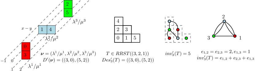
Figure 4. Restricted square strict tableau corresponding to Schur-expansion of an LLT polynomial of three skew shapes.

Using the notation from Fig. 4, let $e_{i,j}(T)$ denote the number of pairs $(\square,\square^{\prime})$ contributing to $\operatorname{inv}_{3}^{\prime}(T)$ with $T(\square)\equiv i$ and $T(\square^{\prime})\equiv j$ modulo $3$, so that

$$\operatorname{inv}_{3}^{\prime}(T)=e_{1,2}(T)+e_{1,3}(T)+e_{2,3}(T).$$

We believe that the following is true:

Conjecture 4.3.

For any triple of skew diagrams $\bm{\nu}=(\lambda^{1}/\mu^{1},\lambda^{2}/\mu^{2},\lambda^{3}/\mu^{3})$ and every triple $\{i,j,k\}=\{1,2,3\}$ with $i<j$, we have

(36) $$\operatorname{LLT}(\lambda^{i}/\mu^{i},\lambda^{j}/\mu^{j})(q)\cdot\operatorname{LLT}(\lambda^{k}/\mu^{k})(q)=\sum_{\lambda}\left(\sum_{\begin{subarray}{c}T\in\operatorname{RSST}(\lambda)\\ \operatorname{Des}_{3}^{\prime}(T)=D^{\prime}(\beta)\\ c(\bm{\nu})\text{ - entries of }T\end{subarray}}q^{e_{i,j}(T)}\right)s_{\lambda}.$$

Corollary 4.4.

Assume that 4.3 holds true. Then 2.7 holds true for all $r$-colored triples of skew shapes.

Proof.

The proof follows the same argument as the one used in Theorem 3.10 to show that

$$[s_{\lambda}]\kappa_{\operatorname{LLT}}(\bm{\nu},f)=\sum_{\begin{subarray}{c}T\in\operatorname{RSST}(\lambda)\\ \operatorname{Des}_{3}^{\prime}(T)=D^{\prime}(\beta)\\ c(\bm{\nu})\text{ - entries of }T\end{subarray}}\mathcal{I}_{(G^{T})_{f}}(q),$$

where $G^{T}$ is an $f$-colored graph whose vertices are entries of $T$ and we connect pairs contributing to $\operatorname{inv}_{3}^{\prime}(T)$. ∎

Note that the above argument works for any $r$-colored tuple of shapes $(\bm{\nu},f)$ and thus, 2.7 suggests the following interesting structure of the coefficients of LLT-polynomials in the Schur expansion.

Problem 4.5.

Let $\bm{\nu}=(\lambda^{1}/\mu^{1},\dots,\lambda^{r}/\mu^{r})$ be an $r$-tuple of skew Young diagrams. Is it true that for any partition $\lambda$ there exists a class of graphs $\mathcal{G}^{\bm{\nu}}_{\lambda}$ with the set of vertices $[1..r]$ such that for any set-partition $\pi\in\mathcal{P}([1..r])$ one has

$$[s_{\lambda}]\prod_{B\in\pi}\operatorname{LLT}^{\operatorname{cospin}}((\bm{\nu})^{B})=\sum_{G\in\mathcal{G}^{\bm{\nu}}_{\lambda}}q^{\sum_{B\in\pi}e_{B}},$$

where $(\bm{\nu})^{B}:=(\bm{\nu},\operatorname{id}_{[1..r]})^{B}$ and $\operatorname{id}_{[1..r]}\colon[1..r]\to[1..r]$ is the identity function?

Note that the affirmative answer for this problem implies 2.7 providing its combinatorial interpretation:

$$[s_{\lambda}]\kappa_{\operatorname{LLT}^{\operatorname{cospin}}}(\bm{\nu},f)=\sum_{G\in\mathcal{G}^{\bm{\nu}}_{\lambda}}\mathcal{I}_{(G)_{f}}(q).$$

In the next section, we show that 4.5 has an affirmative answer in some special cases and thus, 2.7 holds true for them.

4.1. Unicellular LLT and melting lollipops

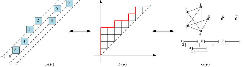
Figure 5. The correspondence between unicellular LLT polynomials, Dyck paths and unit interval graphs. The graph $G(\bm{\nu})$ on the right is the melting lollipop graph $L^{(2)}_{(5,2)}$ and we display the arrangment of unit intervals which realizes it as the unit interval graph.

A Schröder path of length $n$ is a path from $(0,0)$ to $(n,n)$ composed of steps $\uparrow\ =(0,1)$, $\rightarrow\ =(1,0)$, and $\nearrow\ =(1,1)$ (referred to as north, east, and diagonal steps, respectively), which stays above the main diagonal (i.e., it can touch it, but the diagonal steps lie strictly above it). Denote by $(i,j)$ the coordinates of the $1\times 1$ box with upper right vertex in $(i,j)$. It is well known [Hag08] that the vertical-shape LLT polynomials of homogenous degree $n$ are in bijection with Schröder paths of length $n$: start from an $\ell$-tuple of vertical shapes $\bm{\nu}$ of size $n$, label its boxes by their shifted contents and standardize them, i.e. replace them (in the unique way) by labels in $[1..n]$ such that the order of new labels is the same as the order of shifted contents. Now construct a Schröder path $F(\bm{\nu})$ such that the box $(i,j)$ lies below the path if and only if the entry $i$ attacks the entry $j$ in $\bm{\nu}$ and the box $(i,j)$ lies on the diagonal step if the entry $j$ lies directly below the entry $i$. This procedure is clearly invertible and we denote by $\bm{\nu}(F)$ the tuple of vertical strips associated with the Schröder path $F$ (see the left side of Fig. 5 and consult [Hag08] for more details).

A special case of a Schröder path is a Dyck path, that is a path with no diagonal steps. The corresponding $\ell$-tuple of vertical shapes $\bm{\nu}$ of size $n$ is a sequence of $n$ single boxes (i.e. $\ell=n$) and its LLT polynomial is called unicellular. It is remarkable that the LLT graphs associated with unicellular LLT polynomials are precisely unit interval graphs, i.e. they can be realized as the intersection graphs of $n$ unit intervals on the line (see the right side of Fig. 5).

Note that for every unit interval graph $G$ on $n$ vertices, one has

$$\operatorname{LLT}(G)(1)=e_{1}^{n}=\sum_{\lambda\vdash n}\sum_{T\in\operatorname{SYT}(\lambda)}s_{\lambda}.$$

Therefore, it is natural to look for a statistic $a_{G}:\operatorname{SYT}\to\mathbb{N}$ such that

$$[s_{\lambda}]\operatorname{LLT}(G)(q)=\sum_{T\in\operatorname{SYT}(\lambda)}q^{a_{G}(T)}.$$

Recall that the descent set $\operatorname{Des}(T)$ of a standard Young tableau $T\in\operatorname{SYT}(\lambda)$ is given by the values $i\in[1..n-1]$ for which the entry $i+1$ lies in $T$ in a row above the entry $i$ and define

$$\overleftarrow{\operatorname{Des}(T)}:=\{n+1-i\colon i\in\operatorname{Des}(T)\}.$$

Let $m\geq 1,n$ be nonnegative integers and $0\leq k\leq m-1$. A melting lollipop $L_{(m,n)}^{(k)}$ is a graph with the vertex set $[1..m+n]$, built by joining the complete graph on vertices $[1..m]$ with the path on vertices $[m..m+n]$ (with edges of the form $(i,i+1)$) and erasing edges $(1,m),(2,m),\dots,(k,m)$. The unit interval graph depicted in Fig. 5 is the melting lollipop $L^{(2)}_{(5,2)}$.

Recently Huh, Nam and Yoo proved the following theorem [HNY20]:

Theorem 4.6.

[HNY20] Let $\mathcal{F}_{n}$ be the family of unit interval graphs with $n$ vertices such that

$$\operatorname{LLT}(G)(q)=\sum_{\lambda\vdash n}\sum_{T\in\operatorname{SYT}(\lambda)}q^{\sum_{i\in\overleftarrow{\operatorname{Des}(T)}}\deg^{G}_{\operatorname{in}}(i)}s_{\lambda}$$

for each $G\in\mathcal{F}_{n}$ (here $\deg^{G}_{\operatorname{in}}(i)$ denotes the number of edges in $G$ incoming to the vertex $i$). Then $\mathcal{F}_{n}$ contains melting lollipops and their disjoint unions.

Melting lollipops contain two extremal cases for which Theorem 4.6 is a classical result: the complete graph $K_{n}=L_{(n,0)}^{(0)}$ and the path graph $P_{n}=L_{(1,n-1)}^{(0)}=L_{(2,n-2)}^{(0)}$.

Theorem 4.7.

Let $G$ be a melting lollipop graph with $r$ vertices. Then for every set-partition $\pi\in\mathcal{P}([1..r])$, one has

$$[s_{\lambda}]\prod_{B\in\pi}\operatorname{LLT}^{\operatorname{cospin}}(G|_{B})=\sum_{T\in\operatorname{SYT}(\lambda)}q^{\sum_{B\in\pi}e_{B}(G_{\operatorname{in}}^{\overleftarrow{\operatorname{Des}(T)}})},$$

where $G_{\operatorname{in}}^{A}$ is a graph obtained from $G$ by removing all the edges which are not incoming to vertices in $A\subset V$. In particular, 4.5 and 2.7 have an affirmative answer in this case and

$$[s_{\lambda}]\kappa_{\operatorname{LLT}^{\operatorname{cospin}}}(G,f)=\sum_{T\in\operatorname{SYT}(\lambda)}\mathcal{I}_{(G_{\operatorname{in}}^{\overleftarrow{\operatorname{Des}(T)}})_{f}}(q).$$

Proof.

It is enough to notice that

• for every set-partition $\pi\in\mathcal{P}([1..r])$ the graph $G_{\pi}:=\bigoplus_{B\in\pi}G|_{V_{B}}$ is a disjoint union of melting lollipops so that

  $$\prod_{B\in\pi}\operatorname{LLT}(G|_{V_{B}})(q)=\operatorname{LLT}(G_{\pi})(q)=\sum_{\lambda\vdash n}\sum_{T\in\operatorname{SYT}(\lambda)}q^{\sum_{i\in\overleftarrow{\operatorname{Des}(T)}}\deg^{G_{\pi}}_{\operatorname{in}}(i)}s_{\lambda};$$

• the identity

  $$\sum_{i\in A}\deg^{G}_{\operatorname{in}}(i)=|E(G_{\operatorname{in}}^{A})|$$

  follows directly from the construction of $G_{\operatorname{in}}^{A}$.

∎

Remark 4.8.

Note that the class $\mathcal{F}_{n}$ is strictly smaller than the class of unit interval graphs on $n$ vertices which can be seen already for $n=4$: the unit interval graph $G=(V=[1..4],E)$ with $E=\{(1,2),(2,3),(2,4),(3,4)\}$ does not belong to $\mathcal{F}_{n}$. On the other hand, we were not able to find any graph which belongs to $\mathcal{F}_{n}$ and is not a disjoint union of melting lollipops, and it is tempting to conjecture that these two classes of graphs coincide.

We finish by discussing a different approach to attacking 2.7. One can try to find an explicit formula for $\kappa_{\operatorname{LLT}^{\operatorname{cospin}}}(\bm{\nu},f)$ as a linear combination of LLT polynomials with coefficients in $\mathbb{Z}_{\geq 0}[q,q^{-1}]$. Note that Schur polynomials are a special case of LLT polynomials so 2.7 claims that such an expression exists. Nevertheless, we want to stress out that LLT polynomials are not linearly independent so one can hope that some expressions are more natural and easier than others. One particular example where we observed such a natural combinatorial expression is the unicellular case corresponding to the complete graph, i.e., when $\bm{\nu}$ is an $r$-colored tuple of $r$ single boxes: $\lambda^{i}=(1),\mu^{i}=\emptyset$ for all $1\leq i\leq r$. This case might seem to be trivial at first sight, but one can quickly convince oneself that this is a false impression. It turned out that the corresponding cumulant involves beautiful combinatorial objects such as parking functions and it has a form similar to the formula in the Shuffle Theorem, conjectured in [HHL⁺05b] and proved by Carlson and Mellit [CM18]. Before we show the formula we quickly explain what parking functions are.

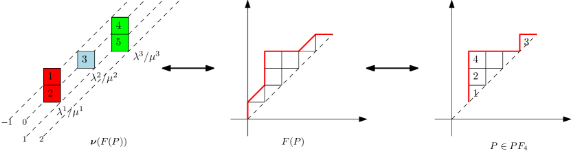
Figure 6. The correspondence between tuples of vertical shapes, Schröder paths and parking functions.

A parking function $P\in\operatorname{PF}_{n-1}$ of size $n-1$ is a function $P\colon[1..n-1]\to[1..n-1]$ such that for each $i\in[1..n-1]$, one has $|P^{-1}(i)|\geq i$. One can represent a parking function by drawing a Dyck path from $(1,1)$ to $(n,n)$ and labeling the boxes to the right of north steps by distinct integers $[1..n-1]$ in such a way that the labels of boxes stacked in the same column are upward increasing. Starting from a parking function $P\in\operatorname{PF}_{n-1}$, convert the corresponding Dyck path of length $n-1$ into a Schröder path of length $n$ by adding steps $\uparrow,\rightarrow$ starting from $(0,0)$ and then replacing all the pairs of consecutive steps $(\rightarrow,\uparrow)$ by $\nearrow$, see the right side of Fig. 6. The following formula was recently proved by the second author:

Theorem 4.9.

[Kow20] Let $(\bm{\nu},f)=(((1),\dots,(1)),f)$ be an $r$-colored tuple of $r$ single boxes. Then

(37) $$\kappa_{\operatorname{LLT}}(\bm{\nu},f)=\kappa_{\operatorname{LLT}^{\operatorname{cospin}}}(\bm{\nu},f)=\sum_{P\in\operatorname{PF}_{r-1}}\operatorname{LLT}(\bm{\nu}(F(P))),$$

where we sum over all parking functions of size $r-1$.

This formula gives a positive expression in terms of vertical-shaped LLT polynomials, which are Schur-positive (by [GH07]) and $e$-positive after applying the shift (by [D’A20, AS22]). In particular, Theorem 4.9 gives yet another proof of 2.7 and also 2.6 in this special case. Although Theorem 4.9 might suggest that there is a combinatorial formula expressing an LLT cumulant as a positive combination of LLT polynomials, we were not able to find a pattern allowing us to construct such a formula in general and we leave this problem for further investigations in the future.

References

- [Ale21] Per Alexandersson, LLT polynomials, elementary symmetric functions and melting lollipops, J. Algebraic Combin. 53 (2021), no. 2, 299–325. MR 4238181
- [AMRV19] T. Abdelgadir, A. Mellit, and F. Rodriguez Villegas, The Tutte polynomial and toric Nakajima quiver varieties, Preprint arXiv:1910.01633, 2019.
- [AN21] Alex Abreu and Antonio Nigro, A symmetric function of increasing forests, Forum Math. Sigma 9 (2021), Paper No. e35, 21. MR 4252214
- [AP18] Per Alexandersson and Greta Panova, LLT polynomials, chromatic quasisymmetric functions and graphs with cycles, Discrete Math. 341 (2018), no. 12, 3453–3482. MR 3862644
- [AS22] Per Alexandersson and Robin Sulzgruber, A combinatorial expansion of vertical-strip LLT polynomials in the basis of elementary symmetric functions, Adv. Math. 400 (2022), Paper No. 108256, 58. MR 4385139
- [Ber17] François Bergeron, Open questions for operators related to rectangular Catalan combinatorics, J. Comb. 8 (2017), no. 4, 673–703. MR 3682396
- [Bla16] Jonah Blasiak, Haglund’s conjecture on 3-column Macdonald polynomials, Math. Z. 283 (2016), no. 1-2, 601–628. MR 3489082
- [CBVdB04] William Crawley-Boevey and Michel Van den Bergh, Absolutely indecomposable representations and Kac-Moody Lie algebras, Invent. Math. 155 (2004), no. 3, 537–559, With an appendix by Hiraku Nakajima. MR 2038196
- [CD22] Guillaume Chapuy and Maciej Dołęga, Non-orientable branched coverings, -Hurwitz numbers, and positivity for multiparametric Jack expansions, Adv. Math. 409 (2022), Paper No. 108645, 1–72.
- [CM18] Erik Carlsson and Anton Mellit, A proof of the shuffle conjecture, J. Amer. Math. Soc. 31 (2018), no. 3, 661–697. MR 3787405
- [D’A20] Michele D’Adderio, -positivity of vertical strip LLT polynomials, J. Combin. Theory Ser. A 172 (2020), 105212, 15. MR 4054520
- [DF17] Maciej Dołęga and Valentin Féray, Cumulants of Jack symmetric functions and the -conjecture, Trans. Amer. Math. Soc. 369 (2017), no. 12, 9015–9039. MR 3710651
- [Doł17] Maciej Dołęga, Strong factorization property of Macdonald polynomials and higher-order Macdonald’s positivity conjecture, J. Algebraic Combin. 46 (2017), no. 1, 135–163. MR 3666415
- [Doł19] Maciej Dołęga, Macdonald cumulants, -inversion polynomials and -parking functions, European J. Combin. 75 (2019), 172–194. MR 3862962
- [ELW10] Eric Egge, Nicholas A. Loehr, and Gregory S. Warrington, From quasisymmetric expansions to Schur expansions via a modified inverse Kostka matrix, European J. Combin. 31 (2010), no. 8, 2014–2027. MR 2718279
- [F1́5] Valentin Féray, Cyclic inclusion-exclusion, SIAM J. Discrete Math. 29 (2015), no. 4, 2284–2311. MR 3427040
- [Ges84] Ira M. Gessel, Multipartite -partitions and inner products of skew Schur functions, Combinatorics and algebra (Boulder, Colo., 1983), Contemp. Math., vol. 34, Amer. Math. Soc., Providence, RI, 1984, pp. 289–317. MR 777705
- [Ges95] by same author, Enumerative applications of a decomposition for graphs and digraphs, Discrete Math. 139 (1995), no. 1-3, 257–271, Formal power series and algebraic combinatorics (Montreal, PQ, 1992). MR 1336842
- [GH07] Ian Grojnowski and Mark Haiman, Affine Hecke algebras and positivity of LLT and Macdonald polynomials, Preprint, 2007.
- [GHQR19] Adriano M. Garsia, James Haglund, Dun Qiu, and Marino Romero, -positivity results and conjectures, Preprint arXiv:1904.07912, 2019.
- [GJ96] I. P. Goulden and D. M. Jackson, Connection coefficients, matchings, maps and combinatorial conjectures for Jack symmetric functions, Trans. Amer. Math. Soc. 348 (1996), no. 3, 873–892. MR 1325917 (96m:05196)
- [GT96] A. M. Garsia and G. Tesler, Plethystic formulas for Macdonald q, t-Kostka coefficients, Adv. Math. 123 (1996), no. 2, 144–222.
- [Hag08] James Haglund, The ,-Catalan numbers and the space of diagonal harmonics, University Lecture Series, vol. 41, American Mathematical Society, Providence, RI, 2008, With an appendix on the combinatorics of Macdonald polynomials. MR 2371044
- [Hai01] Mark Haiman, Hilbert schemes, polygraphs and the Macdonald positivity conjecture, J. Amer. Math. Soc. 14 (2001), no. 4, 941–1006. MR 1839919
- [HHL05a] J. Haglund, M. Haiman, and N. Loehr, A combinatorial formula for Macdonald polynomials, J. Amer. Math. Soc. 18 (2005), no. 3, 735–761. MR 2138143
- [HHL+05b] J. Haglund, M. Haiman, N. Loehr, J. B. Remmel, and A. Ulyanov, A combinatorial formula for the character of the diagonal coinvariants, Duke Math. J. 126 (2005), no. 2, 195–232. MR 2115257
- [HLRV11] Tamás Hausel, Emmanuel Letellier, and Fernando Rodriguez-Villegas, Arithmetic harmonic analysis on character and quiver varieties, Duke Math. J. 160 (2011), no. 2, 323–400. MR 2852119
- [HNY20] JiSun Huh, Sun-Young Nam, and Meesue Yoo, Melting lollipop chromatic quasisymmetric functions and Schur expansion of unicellular LLT polynomials, Discrete Math. 343 (2020), no. 3, 111728, 21. MR 4033624
- [HS02] Tamás Hausel and Bernd Sturmfels, Toric hyperKähler varieties, Doc. Math. 7 (2002), 495–534. MR 2015052
- [JLuR00] Svante Janson, Tomasz Ł uczak, and Andrzej Rucinski, Random graphs, Wiley Series in Discrete Mathematics and Optimization, vol. 45, Wiley-Interscience, 2000.
- [JV13] Matthieu Josuat-Vergès, Cumulants of the -semicircular law, Tutte polynomials, and heaps, Canad. J. Math. 65 (2013), no. 4, 863–878. MR 3071084
- [KN98] Anatol N. Kirillov and Masatoshi Noumi, Affine Hecke algebras and raising operators for Macdonald polynomials, Duke Math. J. 93 (1998), no. 1, 1–39.
- [Kno97] Friedrich Knop, Integrality of two variable Kostka functions, Journal fur die Reine und Angewandte Mathematik (1997), 177–189.
- [Kow20] Maciej Kowalski, LLT cumulants of unicellular Young diagrams, parking functions and Schur positivity, Preprint arXiv:2011.15080, 2020.
- [KS97] Friedrich Knop and Siddhartha Sahi, A recursion and a combinatorial formula for Jack polynomials, Invent. Math. 128 (1997), no. 1, 9–22. MR 1437493
- [Lee21] Seung Jin Lee, Linear relations on LLT polynomials and their k-Schur positivity for , J. Algebraic Combin. 53 (2021), no. 4, 973–990. MR 4263640
- [LLT97] Alain Lascoux, Bernard Leclerc, and Jean-Yves Thibon, Ribbon tableaux, Hall-Littlewood functions, quantum affine algebras, and unipotent varieties, J. Math. Phys. 38 (1997), no. 2, 1041–1068. MR 1434225
- [LS59] V. P. Leonov and A. N. Shiryaev, On a method of semi-invariants, Theor. Probability Appl. 4 (1959), 319–329. MR 0123345
- [LT00] Bernard Leclerc and Jean-Yves Thibon, Littlewood-Richardson coefficients and Kazhdan-Lusztig polynomials, Combinatorial methods in representation theory (Kyoto, 1998), Adv. Stud. Pure Math., vol. 28, Kinokuniya, Tokyo, 2000, pp. 155–220. MR 1864481
- [LV95] Luc Lapointe and Luc Vinet, A Rodrigues formula for the Jack polynomials and the Macdonald-Stanley conjecture, Internat. Math. Res. Notices 1995 (1995), no. 9, 419–424. MR 1360620 (96i:33018)
- [LV97] by same author, Rodrigues formulas for the Macdonald polynomials, Adv. Math. 130 (1997), no. 2, 261–279. MR 1472319 (99e:05128)
- [Mac88] I. G. Macdonald, A new class of symmetric functions, Publ. IRMA Strasbourg 372 (1988), 131–171.
- [NŚ11] Jonathan Novak and Piotr Śniady, What is a Free Cumulant?, Notices of the AMS 58 (2011), no. 2, 300–301.
- [Rob14] Austin Roberts, Dual equivalence graphs revisited and the explicit Schur expansion of a family of LLT polynomials, J. Algebraic Combin. 39 (2014), no. 2, 389–428. MR 3159257
- [Sah96] Siddhartha Sahi, Interpolation, integrality, and a generalization of Macdonald’s polynomials, Internat. Math. Res. Notices 1996 (1996), no. 10, 457–471.
- [SSW03] A. Schilling, M. Shimozono, and D. E. White, Branching formula for -Littlewood-Richardson coefficients, vol. 30, 2003, Formal power series and algebraic combinatorics (Scottsdale, AZ, 2001), pp. 258–272. MR 1979794
- [SW85] Dennis W. Stanton and Dennis E. White, A Schensted algorithm for rim hook tableaux, J. Combin. Theory Ser. A 40 (1985), no. 2, 211–247. MR 814412
- [The20] The Sage Developers, Sagemath, the Sage Mathematics Software System (Version 9.2), 2020, https://www.sagemath.org.
- [Tom21] Foster Tom, A combinatorial Schur expansion of triangle-free horizontal-strip LLT polynomials, Comb. Theory 1 (2021), Paper No. 14, 28. MR 4396219
- [Tut54] W. T. Tutte, A contribution to the theory of chromatic polynomials, Canadian J. Math. 6 (1954), 80–91. MR 0061366
- [Wei35] Louis Weisner, Abstract theory of inversion of finite series, Trans. Amer. Math. Soc. 38 (1935), no. 3, 474–484.