Capacity Bounds under Imperfect Polarization Tracking

Abstract

In optical fiber communication, due to the random variation of the environment, the state of polarization (SOP) fluctuates randomly with time leading to distortion and performance degradation. The memory-less SOP fluctuations can be regarded as a two-by-two random unitary matrix. In this paper, for what we believe to be the first time, the capacity of the polarization drift channel under an average power constraint with imperfect channel knowledge is characterized. An achievable information rate (AIR) is derived when imperfect channel knowledge is available and is shown to be highly dependent on the channel estimation technique. It is also shown that a tighter lower bound can be achieved when a unitary estimation of the channel is available. However, the conventional estimation algorithms do not guarantee a unitary channel estimation. Therefore, by considering the unitary constraint of the channel, a data-aided channel estimator based on the Kabsch algorithm is proposed, and its performance is numerically evaluated in terms of AIR. Monte Carlo simulations show that Kabsch outperforms the least-square error algorithm. In particular, with complex, Gaussian inputs and eight pilot symbols per block, Kabsch improves the AIR by $0.2$ to $0.35$ bits/symbol throughout the range of studied signal-to-noise ratios.

I Introduction

The growing demand for reliable long-distance communication makes it essential to determine the capacity limits of optical links [1, 2, 3]. The emergence of coherent optical communication systems enabled DSP and polarization-division multiplexing to achieve higher spectral efficiencies. However, higher data rates come with increased sensitivity to impairments such as PMD and SOP fluctuations, which must be tracked dynamically in the receiver [4]. Due to the random variation of both internal and environmental impairments, the SOP fluctuates randomly with time [5]. Previous long-term measurements showed that the SOP drift might vary from days and hours in buried fibers [6, 7] to microseconds in aerial fibers [8, 9, 10].

The conventional DSP solutions for SOP tracking are replete with both blind and data-aided algorithms. The CMA [11], thanks to its low complexity and tolerance to PN, has been widely considered for blind polarization tracking [12, 13, 14]. Many studies have been conducted to overcome the so-called “singularity” problem of CMA [15, 16, 17], where the two estimated channels converge twice to the same polarization. The RDE and its variants were proposed to account for higher-order QAM in [18, 19, 20]. The MMA [21] is also applicable to higher-order modulations. More reliable convergence can be obtained using data-aided algorithms such as LMS, which was adopted for SOP estimation by [13, 22], or standard LS, which has been extensively studied for both wireless and optical applications [23, 24, 25, 26]. While the LMS algorithm performs real-time continuous equalization, LS applies to block-based estimation.

While the DP channel can be represented by a unitary matrix, the majority of the available estimation techniques including LS and LMS have no unitary constraint on the estimated channel, leading to sub-optimal solutions. This makes room for algorithms that provide a unitary estimation of the DP channel. Louchet et al. [27] proposed the Kabsch algorithm [28] as a joint blind PN and PMD estimation method. In [29], a blind modulation-format-independent joint PN and polarization tracking algorithm was proposed, and its performance was compared with the blind Kabsch algorithm.

Depending on the estimation algorithm, the speed of the fluctuations, or the additive noise, the polarization tracking might be imperfect. This makes it relevant to ask how the capacity is affected by such an estimation error? While there are no capacity studies regarding the polarization drift channels, to the best of our knowledge, the literature is replete with fiber capacity results. The first finite capacity limit for the single-wavelength optical channel based on a sort of GN model was introduced in [30, 31], showing a lower bound that increases with the power until it reaches a maximum, and then it decreases due to the NLI. Although different nonlinear models were applied, similar results were reported in [32, 33]. Since the GN model cannot truly describe the NLI [34], some modeled the NLI as a linear time-variant distortion highly correlated over time [35, 36]. This made it possible to counteract NLI using the techniques that were conventionally used for linear impairments (e.g., PN, chromatic dispersion, PMD, and SOP [37, 38, 39]). For example, in [40], a tighter lower bound for single-polarization, dispersion-unmanaged systems was achieved by considering the PN.

In this paper, for the first time, we study the capacity of the polarization drift channel in the presence of imperfect knowledge of the channel (e.g., imperfect polarization tracking). Using the mismatched decoding method, we derive an AIR, which is a lower bound on the capacity, in the presence of a channel estimation error. We show that a unitary estimation of the channel leads to a tighter lower bound, which makes it reasonable to seek unitary estimators. A data-aided version of the Kabsch algorithm is proposed for DP channel estimation, for the first time to the best of our knowledge. We compare Kabsch with an LS algorithm in terms of AIR and show that Kabsch outperforms LS throughout the range of considered SNR. For instance, with only eight pilot symbols per channel and block, Kabsch improves the AIR by at least $0.2$ bits per symbol compared to LS.

Notation: Column vectors are denoted by underlined letters $\underline{x}$ and matrices by uppercase roman letters $\mathrm{X}$. We use bold-face letters $\mathbf{x}$ for random quantities and the corresponding nonbold letters $x$ for their realizations. pdf are denoted as $p_{\mathbf{x}}(x)$ and conditional pdf as $p_{\mathbf{y|x}}(y|x)$, where the subscripts will sometimes be omitted if they are clear from the context. Expectation over random variables is denoted by $\mathbb{E}[\cdot]$. Sets are indicated by uppercase calligraphic letters $\mathcal{X}$. The complex zero-mean circularly symmetric Gaussian distribution of a vector is denoted by $\mathbf{\underline{x}}\sim\mathcal{CN}(0,\Lambda_{\underline{x}})$, where $\Lambda_{\underline{x}}=\mathbb{E}[\mathbf{x}\mathbf{x}^{\dagger}]$ is the covariance matrix. All logarithms are in base two. In the context of matrix operations, $|\cdot|$, $(\cdot)^{T}$, $(\cdot)^{\dagger}$, and $\left\lVert.\right\rVert$ represent the determinant, transpose, conjugate transpose, and Frobenius norm operators, respectively.

II Channel Model and Mutual Information

II-A Channel Model

We consider transmission over $n$ channels in the presence of ASE noise at the receiver. The channel is assumed to be constant during a transmission block of length $N$, and changes randomly and independently between the blocks. The assumption that the channel does not change within a block is consistent with the fact that the SOP drifts at a much slower rate than typical transmission rates in optical links [6, 7] and is well established in optical communications literature [38, 40]. The block length $N$ is chosen based on the application and the drift speed of the channel. In most optical communication systems, there is no feedback channel between the transmitter and the receiver. Therefore, the problem of input distribution optimization, corresponding to the case that the channel is known at the transmitter, is not investigated. It is assumed that PMD is negligible and all channel impairments, including nonlinearities and chromatic dispersion are ideally compensated, with the exception of polarization fluctuation and ASE noise, which are modeled by a unitary matrix and AWGN, respectively.

Since different blocks are independent, we just model the symbols in one transmission block in the following. The transmitted signal in each channel at time $\smash{k=0,\ldots,N-1}$ is an $n$-dimensional random vector $\mathbf{\underline{s}}_{k}$ that takes on values from a set $\mathcal{S}$ of zero-mean constellation points. After filtering and resampling the received signals into one sample per symbol, the vector of received samples $\mathbf{\underline{x}}_{k}$ can be expressed as

$$\mathbf{\underline{x}}_{k}=\mathrm{H}\mathbf{\underline{s}}_{k}+\mathbf{\underline{z}}_{k}$$ (1)

where the $n\times n$ matrix $\mathrm{H}$ represents a MIMO channel and $\mathbf{\underline{z}}_{k}$ denotes the complex ASE noise samples at time $k$, which is assumed to be $\mathcal{CN}(0,\sigma_{z}^{2}\mathrm{I}_{n})$ and independent of $\mathbf{\underline{s}}_{k}$. In the remainder of this paper, we will omit the time index $k$ explicitly for notational convenience. This is possible because the input and noise are independent and identically distributed (i.i.d.) over time. We define the covariance matrix of the input vector as

$$\Lambda_{\underline{s}}=\mathbb{E}_{\mathbf{\underline{s}}}[\mathbf{\underline{s}}\mathbf{\underline{s}}^{\dagger}].$$ (2)

In order to maintain the generality of the results, they are given for an arbitrary number of channels $n$ whenever possible. Thus, the MIMO-AWGN channel (1) can describe a wide range of applications and impairments. However, for the purpose of DP optical channel modeling, we are particularly interested in the special cases of $\smash{n=2}$ and $\mathrm{H}$ being unitary, denoted by $\mathrm{H_{u}}$.

II-B Mutual Information with Perfect Knowledge of Channel at the Receiver

The conditional MI between two random vectors $\mathbf{\underline{s}}$, $\mathbf{\underline{x}}$, when the channel $\smash{\mathbf{H}=\mathrm{H}}$ is given, is defined as [41, Eq. 2.61]

$$I(\mathbf{\underline{s}};\mathbf{\underline{x}})=\mathbb{E}_{\mathbf{\underline{s}},\mathbf{\underline{x}}}\left[\log\left(\frac{p(\mathbf{\underline{x}}|\mathbf{\underline{s}},\mathrm{H})}{p(\mathbf{\underline{x}}|\mathrm{H})}\right)\right].$$ (3)

The capacity of this channel under an average power constraint is [42]

$$C=\max\limits_{p(\mathbf{\underline{s}})}{I}(\mathbf{\underline{s}};\mathbf{\underline{x}})\quad\text{s.t.}\quad\operatorname{tr}(\Lambda_{\underline{s}})\leq P,$$ (4)

where $P$ is the transmission power constraint. For the MIMO-AWGN channel in (1), the channel law given $\mathrm{H}$ and $\underline{s}$ is characterized by the pdf

$$p(\underline{x}|\underline{s},\mathrm{H})=\dfrac{1}{\pi^{n}\sigma_{z}^{2n}}\exp\left(-\frac{\left\lVert\underline{x}-\mathrm{H}\underline{s}\right\rVert^{2}}{\sigma_{z}^{2}}\right).$$ (5)

Then, the pdf of the channel output can be calculated as

$$p(\underline{x}|\mathrm{H})=\mathbb{E}_{\mathbf{\underline{s}}}\left[p\right(\underline{x}|\mathbf{\underline{s}},\mathrm{H})].$$ (6)

Given $\mathrm{H}$, the capacity-achieving distribution of the MIMO-AWGN channel law (5) is $\mathcal{CN}$ [43]. Therefore, assuming $\mathcal{CN}(0,\Lambda_{\underline{s}})$ inputs,

$$p(\underline{x}|\mathrm{H})=\dfrac{1}{\pi^{n}|\Lambda_{\underline{x}}|}\exp\left(-\underline{x}^{{\dagger}}\Lambda_{\underline{x}}^{-1}\underline{x}\right),$$ (7)

where

$$\Lambda_{\underline{x}} =\mathbb{E}_{\mathbf{\underline{x}}}\left[\mathbf{\underline{x}}\mathbf{\underline{x}}^{\dagger}\right]$$

$$=\mathrm{H}\Lambda_{\underline{s}}\mathrm{H}^{\dagger}+\sigma_{z}^{2}\mathrm{I}_{n}$$ (8)

is the covariance matrix of the received samples when the channel is given. The MI of a general MIMO system for a given channel is [43]

$$\centering I(\mathbf{\underline{s}};\mathbf{\underline{x}})=\log\left|\mathrm{I}_{n}+\mathrm{H}^{{\dagger}}\mathrm{H}\mathrm{Q}\right|,\@add@centering$$ (9)

where

$$\mathrm{Q}=\Lambda_{\underline{s}}/\sigma_{z}^{2},$$ (10)

and hence $\smash{\operatorname{tr}(\mathrm{Q})\leq n\eta}$, where $\smash{\eta=P/(n\sigma_{z}^{2})}$ is the SNR of each channel. If the channel matrix $\mathrm{H}$ is confined to the set of unitary matrices (i.e., $\mathrm{H}=\mathrm{H_{u}}$), (9) gives

$$I(\mathbf{\underline{s}};\mathbf{\underline{x}})=\log\left|\mathrm{I}_{n}+\mathrm{Q}\right|.$$ (11)

The capacity of a unitary MIMO-AWGN channel is the supremum of (11) for all possible $\mathrm{Q}$. In general, $\mathrm{Q}$ needs to be optimized for each realization of the channel $\mathrm{H}$, if it is known at the transmitter; however, based on (11), the MI is independent of $\mathrm{H}$. Since maximizing (11) is equivalent to maximizing $|\smash{\mathrm{I}_{n}+\mathrm{Q}}|$ and $\mathrm{Q}$ is positive definite, the nondiagonal elements of $\mathrm{Q}$ must be zero, yielding $\mathrm{Q}$ to be a diagonal positive definite matrix. From the well-known theorem that the geometric mean is always upper-bounded by the arithmetic mean, it is straight-forward to show that uniform power distribution at the transmitter (i.e., $\smash{\mathrm{Q}=\eta\mathrm{I}_{n}}$) maximizes (11). Thus, the capacity of an $n$-dimensional unitary MIMO-AWGN channel, still assuming that the channel is perfectly known at the receiver, is

$$\centering C=n\log\left(1+\eta\right).\@add@centering$$ (12)

The capacity of the DP channel is given by simply setting $\smash{n=2}$ in (12).

For a uniform input distribution over a given constellation $\mathcal{S}$, the integral in (6) must be replaced by a summation over all the constellation points, i.e.,

$$p(\underline{x}|\mathrm{H})=\sum_{\underline{s}\in\mathcal{S}}{P(\underline{s})p(\underline{x}|\underline{s},\mathrm{H})},$$ (13)

where $P(\underline{s})$ denotes the probability mass function of the input vector and $p(\underline{x}|\underline{s},\mathrm{H})$ is defined in (5). Using (3) and (13), the MI of the channel for a uniformly distributed discrete input can be expressed as

$${I}(\mathbf{\underline{s}};\mathbf{\underline{x}})=\mathbb{E}_{\mathbf{\underline{s}},\mathbf{\underline{x}}}\left[\log\left(\frac{|\mathcal{S}|\exp(-\frac{\left\lVert\mathbf{\underline{x}}-\mathrm{H}\mathbf{\underline{s}}\right\rVert^{2}}{\sigma_{z}^{2}})}{\underset{\underline{s}^{\prime}\in\mathcal{S}}{\sum}\exp(-\frac{\left\lVert\mathbf{\underline{x}}-\mathrm{H}\underline{s}^{\prime}\right\rVert^{2}}{\sigma_{z}^{2}})}\right)\right],$$ (14)

where the expectations can be estimated numerically.

III the Mutual information in presence of Channel Estimation Error

We derived the capacity of the DP channel with the assumption of perfect channel knowledge at the receiver in (12). In this section, we derive a lower bound on the MI of the channel in the presence of an estimation error. As already shown in [43], when the channel is known, the capacity-achieving distribution is a zero-mean $\mathcal{CN}$ input with a power constraint. Thus, keeping the capacity-achieving distribution, i.e., $\smash{\mathbf{\underline{s}}\sim\mathcal{CN}(0,\Lambda_{\underline{s}})}$ seems reasonable for the imperfectly estimated channel as well. To derive the AIR $I_{q}$, which is a lower bound on the MI (3) between $\mathbf{\underline{s}}$ and $\mathbf{\underline{x}}$, the mismatched decoding inequality [44]

$$I(\mathbf{\underline{s}};\mathbf{\underline{x}})\geq I_{q}=\mathbb{E}_{\mathbf{\underline{x}},\mathbf{\underline{s}}}\left[\log\left(\frac{q(\mathbf{\underline{x}}|\mathbf{\underline{s}})}{q(\mathbf{\underline{x}})}\right)\right]$$ (15)

is used, where $q(\cdot)$ stands for the pdf of an auxiliary channel. Note that this inequality holds for an arbitrary distribution of $q(\cdot)$. The mismatched channel law is here assumed to be

$$q(\underline{x}|\underline{s})=p(\underline{x}|\underline{s},\mathrm{\hat{H}}),$$ (16)

which is obtained by replacing $\mathrm{H}$ in (5) with the estimated channel $\mathrm{\hat{H}}$. This leads to

$$q(\underline{x})=p(\underline{x}|\mathrm{\hat{H}}).$$ (17)

Also, the covariance matrix of the auxiliary channel’s output is obtained by replacing $\mathrm{H}$ with $\mathrm{\hat{H}}$ in (II-B), i.e.,

$$\hat{\Lambda}_{\underline{x}}=\hat{\mathrm{H}}\Lambda_{\underline{s}}\hat{\mathrm{H}}^{\dagger}+\sigma_{z}^{2}\mathrm{I}_{n}.$$ (18)

The average AIR when the estimated channel is random can be written as

$$\bar{I}_{q}=\mathbb{E}_{\mathbf{\hat{H}}}[I_{q}]$$ (19)

In the following, we first derive an AIR for the MIMO-AWGN channel model with a fixed channel $\mathrm{H}$ and estimated channel $\mathrm{\hat{H}}$. Then, we extend the derived AIR to $n$-dimensional unitary channels. By assuming a unitary estimate of the channel (i.e., $\smash{\mathrm{\hat{H}}\mathrm{\hat{H}}^{\dagger}=\mathrm{I}_{n}}$), a tighter AIR is derived. Finally, we use (19) to consider a random estimated channel $\mathbf{\hat{H}}$.

Theorem 1

Th:Lower_Bound Consider an arbitrary complex MIMO channel matrix $\mathrm{H}$ and a fixed estimated channel matrix $\mathrm{\hat{H}}$. Defining $\smash{\mathrm{E}=\mathrm{H}-\mathrm{\hat{H}}}$, the AIR is

$$I_{q} =\log\left|\mathrm{I}_{n}+\mathrm{\hat{H}}\mathrm{Q}\mathrm{\hat{H}}^{\dagger}\right|-\frac{1}{\ln{2}}\operatorname{tr}\left(\mathrm{Q}\mathrm{E}^{\dagger}\mathrm{E}\right)$$

$$-\frac{1}{\ln{2}}\operatorname{tr}\left(\mathrm{I}_{n}-\Lambda_{\underline{x}}\hat{\Lambda}_{\underline{x}}^{-1}\right),$$ (20)

where the definitions of $\Lambda_{\underline{x}}$, $Q$, and $\hat{\Lambda}_{\underline{x}}$ can be found in (II-B), (10), and (18), respectively.

Proof:

One may rewrite (15) as

$$I_{q} =\overbrace{-\mathbb{E}_{\mathbf{\underline{x}}}\left[\log q(\mathbf{\underline{x}})\right]}^{A}+\overbrace{\mathbb{E}_{\mathbf{\underline{s}},\mathbf{\underline{x}}}\left[\log q(\mathbf{\underline{x}}|\mathbf{\underline{s}})\right]}^{B}.$$ (21)

Using (7) and (17), given $\mathrm{H}$, the first term $A$ can be calculated as

$$A =-\mathbb{E}_{\mathbf{\underline{x}}}\left[\log\left(\dfrac{1}{\pi^{n}|\hat{\Lambda}_{\underline{x}}|}\exp\left(-\mathbf{\underline{x}}^{{\dagger}}\hat{\Lambda}_{\underline{x}}^{-1}\mathbf{\underline{x}}\right)\right)\right]$$

$$=\log\left(\pi^{n}|\hat{\Lambda}_{\underline{x}}|\right)+\frac{1}{\ln{2}}\mathbb{E}_{\mathbf{\underline{x}}}\left[\mathbf{\underline{x}}^{\dagger}\hat{\Lambda}_{\underline{x}}^{-1}\mathbf{\underline{x}}\right]$$

$$=\log\left(\pi^{n}|\hat{\Lambda}_{\underline{x}}|\right)+\frac{1}{\ln{2}}\operatorname{tr}\left(\Lambda_{\underline{x}}\hat{\Lambda}_{\underline{x}}^{-1}\right),$$ (22)

where the last step follows the cyclic permutation rule of the trace. For the second term, $B$, when $\mathrm{H}$ is given, we use (5) and (16) to obtain

$$B= ~{}\mathbb{E}_{\mathbf{\underline{s}},\mathbf{\underline{x}}}\left[\log\left(\dfrac{1}{\pi^{n}\sigma_{z}^{2n}}\exp\left(-\frac{\left\lVert\mathbf{\underline{x}}-\mathrm{\hat{H}}\mathbf{\underline{s}}\right\rVert^{2}}{\sigma_{z}^{2}}\right)\right)\right]$$

$$= -\log\left(\pi^{n}\sigma_{z}^{2n}\right)-\frac{\mathbb{E}_{\mathbf{\underline{z}},\mathbf{\underline{s}}}\left[\left\lVert(\mathrm{H}-\mathrm{\hat{H}})\mathbf{\underline{s}}+\mathbf{\underline{z}}\right\rVert^{2}\right]}{\sigma_{z}^{2}\ln{2}}$$

$$= -\log\left(\pi^{n}\sigma_{z}^{2n}\right)-\frac{\mathbb{E}_{\mathbf{\underline{s}}}\left[\left\lVert\mathrm{E}\mathbf{\underline{s}}\right\rVert^{2}\right]+\mathbb{E}_{\mathbf{\underline{z}}}\left[\left\lVert\mathbf{\underline{z}}\right\rVert^{2}\right]}{\sigma_{z}^{2}\ln{2}}$$ (23)

$$= -\log\left(\pi^{n}\sigma_{z}^{2n}\right)-\frac{\operatorname{tr}\left(\sigma_{z}^{2}\mathrm{I}_{n}+\mathrm{E}\Lambda_{\underline{s}}\mathrm{E}^{\dagger}\right)}{\sigma_{z}^{2}\ln{2}}$$ (24)

$$= -\log\left(\pi^{n}\sigma_{z}^{2n}\right)-\frac{1}{\ln{2}}\operatorname{tr}\left(\mathrm{I}_{n}+\mathrm{Q}\mathrm{E}^{\dagger}\mathrm{E}\right),$$ (25)

where (23) follows from the fact that $\mathbf{\underline{z}}$ and $\mathbf{\underline{s}}$ are independent, and the cyclic permutation rule of the trace is used in (24). Finally, substituting (22) and (25) into (21) completes the proof. ∎

For the sake of keeping Theorem LABEL:Th:Lower_Bound as general as possible, no assumption is made about the transmitter knowledge of the estimated channel. However, in the context of the optical communications, we are more interested in the case that the transmitter has no channel knowledge. When the channel is not known at the transmitter, the only reasonable choice for $\Lambda_{\underline{s}}$ is to apply uniform power distribution between the channels.

Corollary 1

corollary:1 Assume that the channel is unitary (i.e., $\smash{\mathrm{H}=\mathrm{H_{u}}}$) and that uniform power distribution takes place at the transmitter. Then the AIR of a unitary channel can be written as

$$I_{q} =\log\left|\mathrm{I}_{n}+\eta\mathrm{\hat{H}}\mathrm{\hat{H}}^{\dagger}\right|-\frac{1}{\ln{2}}\operatorname{tr}\left(\eta\mathrm{E}^{\dagger}\mathrm{E}\right)$$

$$-\frac{1}{\ln{2}}\operatorname{tr}\left(\mathrm{I}_{n}-(1+\eta)(\mathrm{I}_{n}+\eta\mathrm{\hat{H}}\mathrm{\hat{H}}^{\dagger})^{-1}\right).$$ (26)

Proof:

The uniform power distribution $\smash{\Lambda_{\underline{s}}=P\mathrm{I}_{n}/n}$ yields $\smash{\mathrm{Q}=\eta\mathrm{I}_{n}}$. Knowing the channel is unitary (i.e., $\smash{\mathrm{H_{u}}\mathrm{H_{u}}^{\dagger}=\mathrm{I}_{n}}$) and using (II-B) and (18), we can write $\smash{\Lambda_{\underline{x}}=\sigma_{z}^{2}(1+\eta)\mathrm{I}_{n}}$ and $\smash{\hat{\Lambda}_{\underline{x}}^{-1}=\sigma_{z}^{-2}(\mathrm{I}_{n}+\eta\mathrm{\hat{H}}\mathrm{\hat{H}}^{\dagger})^{-1}}$. Finally, substituting $\mathrm{Q}$, $\Lambda_{\underline{x}}$, and $\hat{\Lambda}_{x}^{-1}$ in (20) completes the proof. ∎

Corollary 2

corollary:2 Assume that the channel is a fixed unitary matrix $\mathrm{H_{u}}$ and that the estimated channel is an arbitrary random matrix $\smash{\mathbf{\hat{H}}=\mathrm{H_{u}}-\mathbf{E}}$. Then with a uniform power distribution, the average AIR is

$$\bar{I}_{q} =\mathbb{E}_{\mathbf{\hat{H}}}\left[\log\left|\mathrm{I}_{n}+\eta\mathbf{\hat{H}}\mathbf{\hat{H}}^{\dagger}\right|\right]-\frac{1}{\ln{2}}\operatorname{tr}\left(\eta\mathrm{R}_{\mathrm{E}}\right)$$

$$-\frac{1}{\ln{2}}\operatorname{tr}\left(\mathrm{I}_{n}-(1+\eta)\mathbb{E}_{\mathbf{\hat{H}}}\left[(\mathrm{I}_{n}+\eta\mathbf{\hat{H}}\mathbf{\hat{H}}^{\dagger})^{-1}\right]\right),$$ (27)

where

$$\mathrm{R}_{\mathrm{E}} =\mathbb{E}_{\mathbf{E}}[\mathbf{E}^{\dagger}\mathbf{E}].$$ (28)

Proof:

By applying (19) to (1) the proof is complete. ∎

Corollary 3

corollary:3 If $\mathbf{E}$ has a spherically symmetric distribution, then (2) gives the same $\bar{I}_{q}$ for any $\mathrm{H_{u}}$.

Proof:

Since $\mathrm{H_{u}}\mathrm{H_{u}}^{\dagger}=\mathrm{I}_{n}$, we can write

$$\mathbf{\hat{H}}\mathbf{\hat{H}}^{\dagger} =(\mathrm{H_{u}}-\mathbf{E})(\mathrm{H_{u}}-\mathbf{E})^{\dagger}$$

$$=(\mathrm{I}_{n}-\mathbf{E}\mathrm{H_{u}}^{\dagger})(\mathrm{I}_{n}-\mathbf{E}\mathrm{H_{u}}^{\dagger})^{\dagger}$$ (29)

and since $\mathbf{E}$ has a spherically symmetric distribution, it is invariant to rotation. Therefore, for any $\mathrm{H_{u}}$, $\mathbf{E}\mathrm{H_{u}}^{\dagger}$ has the same distribution as $\mathbf{E}$ and $\mathbf{\hat{H}}\mathbf{\hat{H}}^{\dagger}$ has the same distribution as $(\mathrm{I}_{n}-\mathbf{E})(\mathrm{I}_{n}-\mathbf{E})^{\dagger}$. Thus, (2) yields the same AIR independently of $\mathrm{H_{u}}$. ∎

We have not made any assumption on the estimation technique, so the derived lower bounds hold for an arbitrary estimator. It can be seen that (2) highly depends on the choice of estimation technique, so one can tighten the bound by choosing a suitable estimator.

Corollary 4

corollary:4 For a complex unitary channel, a unitary estimated channel, and a uniform power distribution, the AIR is

$$\bar{I}_{q} =n\log(1+\eta)-\frac{\eta}{\ln{2}}\operatorname{tr}(\mathrm{R}_{\mathrm{E}}).$$ (30)

Proof:

By applying $\smash{\mathbf{\hat{H}}\mathbf{\hat{H}}^{\dagger}=\mathrm{I}_{n}}$ to (2) the proof is complete. ∎

Note that (30) is independent of $\mathrm{H}$, meaning that the AIR is the same for any unitary channel. Interestingly, the unitary estimation of the channel removes two terms on the right-hand side of (2), leading to a simpler bound.

For uniformly distributed discrete inputs, the pdf of the output of the auxiliary channel is

$$q(\underline{x})=\sum_{\underline{s}\in\mathcal{S}}{P(\underline{s})q(\underline{x}|\underline{s})},$$ (31)

where $q(\underline{x}|\underline{s})$ is defined in (16). Using (15), (16), and (31), the average AIR for a uniformly distributed discrete input can be expressed as

$$\bar{I}_{q}=\mathbb{E}\left[\log\left(\frac{|\mathcal{S}|\exp(-\frac{\left\lVert\mathbf{\underline{x}}-\mathbf{\hat{H}}\mathbf{\underline{s}}\right\rVert^{2}}{\sigma_{z}^{2}})}{\underset{\underline{s}^{\prime}\in\mathcal{S}}{\sum}\exp(-\frac{\left\lVert\mathbf{\underline{x}}-\mathbf{\hat{H}}\underline{s}^{\prime}\right\rVert^{2}}{\sigma_{z}^{2}})}\right)\right],$$ (32)

where the expectation is over $\mathbf{\underline{s}}$, $\mathbf{\underline{x}}$, and $\mathbf{\hat{H}}$, which can be estimated numerically.

IV Channel Estimation

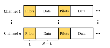
Figure 1: Transmission block model

In this section, first, the well-established LS estimation algorithm is presented. Then, a unitary estimation method is proposed for unitary channels. As illustrated in Fig. 1, to make data-aided channel estimation possible, the first $L$ symbols of the transmission block are pilot symbols $\smash{\mathrm{D}=[\underline{s}_{0},...,\underline{s}_{L-1}]}$, which are assumed to be known at both transmitter and receiver. The optimal pilot assignment $\mathrm{D}$ should have the following properties [45]:

• $\smash{L\geq n}$

• $\smash{\mathrm{D}\mathrm{D}^{\dagger}=\frac{PL}{n}\mathrm{I}_{n}}$

The complex matrix $\smash{\mathbf{X}=[\mathbf{\underline{x}}_{0},...,\mathbf{\underline{x}}_{L-1}]}$ of received symbols is

$$\mathbf{X}=\mathbf{H}_{\mathrm{u}}\mathrm{D}+\mathbf{Z},$$ (33)

where $\smash{\mathbf{Z}\sim\mathcal{CN}(0,\sigma_{z}^{2}\mathrm{I}_{n})}$ is an $\smash{n\times L}$ matrix of i.i.d. noise samples and $\mathbf{H}_{\mathrm{u}}$ is an $\smash{n\times n}$ random unitary channel matrix, which is assumed to remain constant during a transmission block.

Note that the channel estimation problem can be translated to finding a certain number of independent real values, often regarded as the DOF and denoted by $\nu$.

IV-A LS Algorithm

Conventional optical transmission systems often use LMS for a real-time estimate of the channel, because LMS tracks the channel change with each received symbol. However, in this paper it is assumed that the channel is constant during a transmission block and the LS method is well adapted to block based transmissions. The LS estimator estimates the channel by minimizing the squared error between the desired and received signal. For a MIMO-AWGN channel, the LS optimization problem can be expressed as [46]

$$\min\limits_{\mathbf{\hat{H}}}\left\lVert\mathbf{X}-\hat{\mathbf{H}}\mathrm{D}\right\rVert^{2}$$ (34)

Knowing $\mathrm{D}$ and $\mathbf{X}$, the solution of (34) is [46],[47, Ch. 8]

$$\mathbf{\hat{H}}_{\text{LS}}=\mathbf{X}\mathrm{D}^{\dagger}(\mathrm{D}\mathrm{D}^{\dagger})^{-1}$$ (35)

However, the pilots are chosen in such a way that $\smash{\mathrm{D}\mathrm{D}^{\dagger}=\frac{PL}{n}\mathrm{I}_{n}}$. Therefore, we can write

$$\mathbf{\hat{H}}_{\text{LS}}=\frac{n}{PL}\mathbf{X}\mathrm{D}^{\dagger}.$$ (36)

It can be shown that $\mathrm{R_{E}}$ for the LS algorithm is [46]

$$\mathrm{R_{E}}=\mathbb{E}_{\mathbf{E}}\left[\mathrm{\mathbf{E}}^{\dagger}\mathrm{\mathbf{E}}\right]=\frac{n\sigma_{z}^{2}}{PL}\mathrm{I}_{n}=\frac{1}{\eta L}\mathrm{I}_{n}$$ (37)

showing that the estimation error of the LS algorithm is inversely proportional to the SNR and the pilot length $L$.

It is worth mentioning that the LS algorithm has to find $\nu=2n^{2}$ independent real values to make an estimate.

IV-B Kabsch Algorithm

The problem with both blind estimation algorithms (e.g., CMA, RDE, and MMA) and pilot-aided estimation algorithms (e.g., LS and LMS) is that their optimization problems are not adopted for unitary channel estimation, making their solutions suboptimal if $\mathbf{H}$ is known to be unitary. Thus, in this part, we apply the unitary constraint of the channel to the estimation problem of (34) and write

$$\min\limits_{\mathbf{\hat{H}}}\left\lVert\mathbf{X}-\mathbf{\hat{H}}\mathrm{D}\right\rVert^{2}\quad\text{s.t.}\quad\mathbf{\hat{H}}\mathbf{\hat{H}}^{\dagger}=\mathrm{I}_{n}.$$ (38)

The optimal solution to this problem is given by the Kabsch algorithm [28] as

$$\mathbf{\hat{H}}_{\text{Kabsch}}=\mathbf{UV}^{\dagger},$$ (39)

where $\smash{\mathbf{U}\Sigma\mathbf{V}^{\dagger}}$ is the singular value decomposition function of $\mathbf{X}\mathrm{D}^{\dagger}$. As can be seen, unlike the blind conventional estimators, Kabsch is independent of the modulation format of the transmission. The Kabsch algorithm was proposed for optical communication by Louchet et al. [27] as a blind polarization tracking algorithm, where decision-directed symbols were used instead of pilots.

In contrast to LS, no analytical result is known for $\mathrm{R_{E}}$ of the Kabsch algorithm. Although we cannot analytically prove it, we can make an intuitive prediction by considering that $\smash{\nu=n^{2}}$ for a unitary estimation of the channel while for a general estimation of the channel $\smash{\nu=2n^{2}}$. Since the channel estimation problem is equivalent to finding $\nu$ independent real-valued quantities, one can predict that the estimation error of Kabsch would be half of LS. More interestingly, for special unitary channels where $\smash{|\mathrm{H_{u}}|=1}$, the DOF is $\smash{n^{2}-1}$ and the gain by the unitary algorithm can be even higher; however, this gain vanishes for large $n$.

Note that in the case of the DP channel, the singular value decomposition is deployed only on a two-by-two matrix, making it less computationally complex than for higher $n$.

V Numerical Results

In this section, through Monte Carlo trials, the AIR of the DP channel (i.e., $\smash{n=2}$) for the estimation algorithms detailed in Section IV is computed. While AIRs are derived for a fixed channel matrix $\mathrm{H}$, the estimated channel $\mathbf{\hat{H}}$ is dependent on each realization of the channel. A deterministic sequence of $L$ QPSK symbols is selected to satisfy the pilot conditions detailed in Section IV.

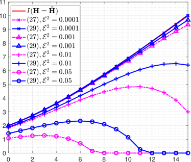
Figure 2: The average AIR $\bar{I}_{q}$ of the DP channel as a function of SNR $\eta$ and estimation error per DOF $\mathcal{E}^{2}$.

Numerical results verify that the estimation error of the Kabsch algorithm completely follows our prediction in Sec. IV-B. Thus, to perform a fair comparison between the unitary and nonunitary estimators, we define a new parameter called estimation error per DOF as $\mathcal{E}^{2}=\operatorname{tr}{\mathrm{R}_{\mathrm{E}}}/(n\nu)$. Note that for a general nonunitary estimator $\nu=2n^{2}$ and for a general unitary estimator $\nu=n^{2}$.

Using $\mathcal{CN}$ inputs, Fig. 2 shows the Monte-Carlo averaged AIR $\bar{I}_{q}$ of the DP channel according to (2) and (30) for $\smash{n=2}$. Note that based on corollary:3, for an estimation error $\mathbf{E}$ with a spherically symmetric distribution, (2) is independent of $\mathrm{H_{u}}$. For the blue curves, we have assumed that $\mathbf{E}$ is distributed according to $\mathcal{CN}(0,\mathrm{R_{E}})$ with $\smash{\mathrm{R}_{\mathrm{E}}=2n^{2}\mathcal{E}^{2}\mathrm{I}_{2}}$. For the dashed magenta curves, $\mathbf{\hat{H}}$ is unitary and $\smash{\mathrm{R}_{\mathrm{E}}=n^{2}\mathcal{E}^{2}}\mathrm{I}_{n}$. The results illustrate that when we have the same $\mathcal{E}^{2}$, the unitary estimate of the channel leads to a higher AIR. Besides, it can be seen that for a constant estimation error per DOF $\mathcal{E}^{2}$, the average AIR reaches a maximum for a specific SNR and then decreases. This can be justified according to the right-hand side of (2) and (30), where the first term increases in a logarithmic manner with respect to SNR, but the second term decreases linearly with SNR. Therefore there is an optimum SNR that maximizes the AIR. This behavior comes from the assumption of a constant $\mathcal{E}^{2}$ regardless of the SNR, which, as we shall see next, is not fully realistic.

Figure 3: The average AIR $\bar{I}_{q}$ when $\smash{L=8}$ DP pilot symbols are used. (a) Using $\mathcal{CN}$ inputs where for LS and Kabsch, $\bar{I}_{q}$ is according to (2) and (30), respectively. (b) Using uniformly distributed DP-$16$-QAM inputs where $\bar{I}_{q}$ for both LS and Kabsch is according to (32).

Fig. 3(a) presents the AIR of LS and Kabsch when $\mathcal{CN}$ inputs are used. The solid red line indicates the receiver perfectly knows the channel. It can be concluded that with $\smash{L=8}$, Kabsch surpasses LS throughout the range of considered SNRs. More specifically, at $4$ and $14$ dB SNRs (see insets), Kabsch has at least $0.2$ and $0.35$ bits per symbol higher AIR, respectively. Additionally, it is clear from the results that LS is upper-bounded by Kabsch, and increasing the SNR cannot fill the gap. This behavior can be justified because, unlike LS, Kabsch guarantees a unitary estimation of the channel leading to a lower estimation error. Moreover, as the SNR increases, the gap between Kabsch and LS and the actual channel MI is almost constant. Since the theoretical gap is $(\eta/\ln{2})\operatorname{tr}(\mathrm{R_{E}})$ according to corollary:4, we conclude that the error covariance $\mathrm{R}_{\mathrm{E}}$ of Kabsch is inversely proportional to the SNR, i.e., $\smash{\mathrm{R}_{\mathrm{E}}\propto{1}/{\eta}}$. Unlike Fig. 2, the AIR bounds are monotonically increasing with SNR which is due to the fact that the estimation error is decreasing with SNR.

A comparison between LS and Kabsch with DP-$16$-QAM inputs is provided in Fig. 3(b). The MI when the channel is perfectly known at the receiver is marked by the solid red line. Evidently, Kabsch outperforms LS throughout the considered range of SNRs. The results also support the fact that Kabsch upper-bounds LS for various inputs, which completely agrees with Fig. 2, where the unitary estimation of the channel leads to a higher AIR.

Figure 4: The average information gap $I-\bar{I}_{q}$ for a range of pilot lengths. (a) $\mathcal{CN}$ inputs where $\bar{I}_{q}$ for LS and Kabsch algorithms is according to (2) and (30), respectively. (b) Uniformly distributed DP-$16$-QAM inputs where $\bar{I}_{q}$ for both LS and Kabsch is according to (32).

Fig. 4 displays the information gap between the AIRs and the capacity of the DP channel, when (a) $\mathcal{CN}$ inputs and (b) DP-$16$-QAM inputs are used. The overall dominance of Kabsch throughout the range of considered SNRs can be easily verified. Evidently, it is beneficial to use higher pilot numbers at low SNRs. Given the fact that $\smash{\mathrm{R}_{\mathrm{E}}\propto{1}/({L\eta})}$ for LS (37) and that Kabsch in Fig. 4 follows the same trend with respect to $L$, we can empirically conclude that $\mathrm{R_{E}}$ of Kabsch is also inversely proportional to the pilot length and the SNR.

It is beneficial to use Kabsch to limit the rate loss due to the pilots. For example, a reasonable performance is achieved by only a block of $\smash{L=16}$ pilot symbols, which is relatively small compared to the transmission block size in optical communication systems, implying that the rate loss is negligible. For instance, for a system operating at a rate of $28$ Gbaud, even if the channel remains constant for one microsecond (i.e., the SOP drift time is one microsecond), it corresponds to a block length $N$ of at least $28,000$ symbols and the rate loss due to $16$ pilots is negligible.

VI Conclusion

The capacity of unitary MIMO-AWGN channels and specifically DP was investigated. With perfect channel knowledge, the capacity of unitary channels is the same as for the regular AWGN channel. An AIR with imperfect channel knowledge was derived and showed that the AIR is highly dependent on the estimation algorithm. In the case of unitary channels, higher AIR are obtained with a unitary estimation of the channel. The bounds are derived for any $\smash{n\geq 2}$ dimensions, meaning that the results can be applied to other optical channels. In particular, Th:Lower_Bound can be directly applied to space-division multiplexed channels which are impaired with polarization- and mode-dependent loss. In contrast to the conventional estimation algorithms, the proposed data-aided Kabsch algorithm ensures a unitary estimate of the channel. Numerical results showed that for various input distributions, Kabsch outperforms LS in terms of AIR. Also, like LS, Kabsch can perform very well with only a few pilot symbols, making the transmission rate loss due to the pilots negligible.

References

- [1] D. Monroe, “Optical fibers getting full,” Commun. ACM, vol. 59, no. 10, pp. 10–12, Sep. 2016.
- [2] E. Agrell, A. Alvarado, and F. R. Kschischang, “Implications of information theory in optical fiber communications,” Philos. Trans. R. Soc. A, vol. 374, Mar. 2016.
- [3] R.-J. Essiambre, G. J. Foschini, P. J. Winzer, G. Kramer, and B. Goebel, “Capacity limits of optical fiber networks,” J. Lightwave Technol., vol. 28, pp. 662–701, Feb. 2010.
- [4] S. J. Savory, “Digital coherent optical receivers: Algorithms and subsystems,” IEEE J. Sel. Topics Quantum Electron., vol. 16, no. 5, pp. 1164–1179, Sep.-Oct. 2010.
- [5] C. D. Poole and C. R. Giles, “Polarization-dependent pulse compression and broadening due to polarization dispersion in dispersion-shifted fiber,” Opt. Lett., vol. 13, no. 2, pp. 155–157, Feb. 1988.
- [6] M. Karlsson, J. Brentel, and P. A. Andrekson, “Long-term measurement of PMD and polarization drift in installed fibers,” J. Lightwave Technol., vol. 18, no. 7, pp. 941–951, Jul. 2000.
- [7] C. T. Allen, P. K. Kondamuri, D. L. Richards, and D. C. Hague, “Measured temporal and spectral PMD characteristics and their implications for network-level mitigation approaches,” J. Lightwave Technol., vol. 21, no. 1, pp. 79–86, Jan. 2003.
- [8] D. Waddy, P. Lu, L. Chen, and X. Bao, “Fast state of polarization changes in aerial fiber under different climatic conditions,” IEEE Photon. Technol. Lett., vol. 13, no. 9, pp. 1035–1037, Sep. 2001.
- [9] P. M. Krummrich, D. Ronnenberg, W. Schairer, D. Wienold, F. Jenau, and M. Herrmann, “Demanding response time requirements on coherent receivers due to fast polarization rotations caused by lightning events,” Opt. Express, vol. 24, no. 11, pp. 12 442–12 457, May 2016.
- [10] Z. Zhang, X. Bao, Q. Yu, and L. Chen, “Fast state of polarization and PMD drift in submarine fibers,” IEEE Photon. Technol. Lett., vol. 18, no. 9, pp. 1034–1036, May 2006.
- [11] D. Godard, “Self-recovering equalization and carrier tracking in two-dimensional data communication systems,” IEEE Trans. on Commun., vol. 28, no. 11, pp. 1867–1875, Nov. 1980.
- [12] S. J. Savory, G. Gavioli, R. I. Killey, and P. Bayvel, “Transmission of 42.8 Gbit/s polarization multiplexed NRZ-QPSK over km of standard fiber with no optical dispersion compensation,” in Proc. Opt. Fiber Commun. Conf. (OFC), 2007, p. OTuA1.
- [13] S. J. Savory, “Digital filters for coherent optical receivers,” Opt. Express, vol. 16, no. 2, pp. 804–817, Jan. 2008.
- [14] K. Kikuchi, “Polarization-demultiplexing algorithm in the digital coherent receiver,” in Proc. IEEE/LEOS Summer Topical Meetings, 2008, pp. 101–102.
- [15] ——, “Performance analyses of polarization demultiplexing based on constant-modulus algorithm in digital coherent optical receivers,” Opt. Express, vol. 19, no. 10, pp. 9868–9880, May 2011.
- [16] L. Liu, Z. Tao, W. Yan, S. Oda, T. Hoshida, and J. C. Rasmussen, “Initial tap setup of constant modulus algorithm for polarization de-multiplexing in optical coherent receivers,” in Proc. Opt. Fiber Commun. Conf. (OFC), Mar. 2009, p. OMT2.
- [17] M. S. Faruk, Y. Mori, C. Zhang, and K. Kikuchi, “Proper polarization demultiplexing in coherent optical receiver using constant modulus algorithm with training mode,” in Proc. OptoElectron. Commun. Conf. (OECC), 2010, pp. 768–769.
- [18] M. Ready and R. Gooch, “Blind equalization based on radius directed adaptation,” in Proc. Int. Conf. Acoust. Speech Sig. Process. (ICASSP), vol. 3, Apr. 1990, pp. 1699–1702.
- [19] I. Fatadin, D. Ives, and S. J. Savory, “Blind equalization and carrier phase recovery in a 16-QAM optical coherent system,” J. Lightwave Technol., vol. 27, no. 15, pp. 3042–3049, Aug. 2009.
- [20] D. Lavery, M. Paskov, R. Maher, S. J. Savory, and P. Bayvel, “Modified radius directed equaliser for high order QAM,” in Proc. Eur. Conf. Opt. Commun. (ECOC), Sep. 2015, p. We4D5.
- [21] J. Yang, J.-J. Werner, and G. Dumont, “The multimodulus blind equalization and its generalized algorithms,” IEEE J. Sel. Areas Commun., vol. 20, no. 5, pp. 997–1015, Jun. 2002.
- [22] C. R. S. Fludger, T. Duthel, D. van den Borne, C. Schulien, E.-D. Schmidt, T. Wuth, J. Geyer, E. De Man, G.-D. Khoe, and H. de Waardt, “Coherent equalization and POLMUX-RZ-DQPSK for robust 100-GE transmission,” J. Lightwave Technol., vol. 26, no. 1, pp. 64–72, Jan. 2008.
- [23] I. Barhumi, G. Leus, and M. Moonen, “Optimal training design for MIMO OFDM systems in mobile wireless channels,” IEEE Trans. Signal Process., vol. 51, no. 6, pp. 1615–1624, June 2003.
- [24] E. Ip and J. M. Kahn, “Digital equalization of chromatic dispersion and polarization mode dispersion,” J. Lightwave Technol., vol. 25, no. 8, pp. 2033–2043, Aug. 2007.
- [25] W. Shieh, “Maximum-likelihood phase and channel estimation for coherent optical OFDM,” IEEE Photon. Technol. Letters, vol. 20, no. 8, pp. 605–607, Apr. 2008.
- [26] M. Kuschnerov, M. Chouayakh, K. Piyawanno, B. Spinnler, E. de Man, P. Kainzmaier, M. S. Alfiad, A. Napoli, and B. Lankl, “Data-aided versus blind single-carrier coherent receivers,” IEEE Photon. Journal, vol. 2, no. 3, pp. 387–403, June 2010.
- [27] H. Louchet, K. Kuzmin, and A. Richter, “Joint carrier-phase and polarization rotation recovery for arbitrary signal constellations,” IEEE Photon. Technol. Lett., vol. 26, no. 9, pp. 922–924, May 2014.
- [28] W. Kabsch, “A solution for the best rotation to relate two sets of vectors,” Acta Crystallographica Section A, vol. 32, no. 5, pp. 922–923, Sep. 1976.
- [29] C. B. Czegledi, E. Agrell, M. Karlsson, and P. Johannisson, “Modulation format independent joint polarization and phase tracking for coherent receivers,” J. Lightwave Technol., vol. 34, no. 14, pp. 3354–3364, Jul. 2016.
- [30] A. Splett, C. Kurtzke, and K. Petermann, “Ultimate transmission capacity of amplified optical fiber communication systems taking into account fiber nonlinearities,” in Proc. Eur. Conf. Opt. Commun. (ECOC), 1994, pp. 41–44.
- [31] C. Kurtzke, “Kapazitätsgrenzen digitaler optischer Übertragungssysteme,” Doctoral Thesis (in German), Technische Universität Berlin, Berlin, Germany, 1995. [Online]. Available: http://doi.org/10.14279/depositonce-5080
- [32] A. G. Green, P. B. Littlewood, P. P. Mitra, and L. G. L. Wegener, “Schrödinger equation with a spatially and temporally random potential: Effects of cross-phase modulation in optical communication,” Phys. Rev. E, vol. 66, p. 046627, Oct. 2002.
- [33] P. P. Mitra and J. B. Stark, “Nonlinear limits to the information capacity of optical fiber communications,” Nature, vol. 411, pp. 1027–1030, June 2001.
- [34] E. Agrell, A. Alvarado, G. Durisi, and M. Karlsson, “Capacity of a nonlinear optical channel with finite memory,” J. Lightwave Technol., vol. 32, no. 16, pp. 2862–2876, Aug. 2014.
- [35] M. Secondini and E. Forestieri, “Analytical fiber-optic channel model in the presence of cross-phase modulation,” IEEE Photon. Technol. Lett., vol. 24, no. 22, pp. 2016–2019, Nov. 2012.
- [36] M. Secondini, E. Forestieri, and G. Prati, “Achievable information rate in nonlinear WDM fiber-optic systems with arbitrary modulation formats and dispersion maps,” J. Lightwave Technol., vol. 31, no. 23, pp. 3839–3852, Dec. 2013.
- [37] M. Secondini and E. Forestieri, “On XPM mitigation in WDM fiber-optic systems,” IEEE Photon. Technol. Lett., vol. 26, no. 22, pp. 2252–2255, Nov. 2014.
- [38] R. Dar, M. Feder, A. Mecozzi, and M. Shtaif, “Time varying ISI model for nonlinear interference noise,” in Proc. Opt. Fiber Commun. Conf. (OFC), Mar. 2014, p. W2A.62.
- [39] ——, “Inter-channel nonlinear interference noise in WDM systems: Modeling and mitigation,” J. Lightwave Technol., vol. 33, no. 5, pp. 1044–1053, Mar. 2015.
- [40] R. Dar, M. Shtaif, and M. Feder, “New bounds on the capacity of the nonlinear fiber-optic channel,” Opt. Lett., vol. 39, no. 2, pp. 398–401, Jan. 2014.
- [41] T. M. Cover and J. A. Thomas, Elements of Information Theory, 2nd ed. Hoboken, NJ, USA: Wiley, Jul. 2006.
- [42] C. E. Shannon, “A mathematical theory of communication,” Bell Syst. Tech. J., vol. 27, no. 3, pp. 379–423/623–656, Jul., Oct. 1948.
- [43] E. Telatar, “Capacity of multi-antenna Gaussian channels,” Eur. Trans. Telecommun., vol. 10, no. 6, pp. 585–595, Nov.–Dec. 1999.
- [44] E. Agrell, “Capacity bounds in optical communications,” in Proc. Eur. Conf. Opt. Commun. (ECOC), Sep. 2017.
- [45] B. Hassibi and B. Hochwald, “How much training is needed in multiple-antenna wireless links?” IEEE Trans. Inform. Theory, vol. 49, no. 4, pp. 951–963, Apr. 2003.
- [46] M. Biguesh and A. Gershman, “Training-based MIMO channel estimation: a study of estimator tradeoffs and optimal training signals,” IEEE Trans. on Signal Process., vol. 54, no. 3, pp. 884–893, Mar. 2006.
- [47] S. M. Kay, Fundamentals of Statistical Signal Processing: Estimation Theory. Englewood Cliffs: NJ: Prentice-Hall, 1993.