Causal Temporal Renormalisation Group Flow of the Energy-Momentum Tensor

Abstract

We derive the temporal renormalisation group flow of the energy-momentum tensor at the example of a general scalar theory. The local causal structure of the temporal renormalisation group flow allows to monitor and control causality, unitarity and general conservation laws at each infinitesimal renormalisation group step. We explore energy-conserving truncations in a comparison of generic flows and the causal temporal flow of the energy-momentum tensor. We also observe that the temporal regulator preserves scale invariance, which is violated for generic momentum regulators. Specifically we discuss the relation of these terms to the trace anomaly of the energy-momentum tensor. Moreover, we show that the causal temporal flow of the energy-momentum tensor can be integrated analytically, and demonstrate, that the result is consistent with energy conservation.

I Introduction

Understanding the time evolution of quantum field theories in and out of equilibrium is relevant for a variety of different physical systems ranging from inflationary cosmology over the dynamics of phase transitions in the standard model and heavy ion collisions to table top experiments with ultracold atoms.

The framework of the temporal functional renormalisation group (t-fRG) constitutes a manifestly causal approach that gives access to the dynamics of correlation functions in quantum field theories Gasenzer and Pawlowski (2008); Gasenzer et al. (2010); Corell et al. (2021). As opposed to standard flows in momentum space with imaginary time, the t-fRG flow is a real-time flow. Causality is ensured by a causal temporal regulator, that suppresses all quantum fluctuations beyond the cutoff time $\tau$, hence terminating the Keldysh time contour at the cutoff time.

In the present work we discuss the time evolution of the energy-momentum tensor (EMT). The EMT carries some of the most important conservation laws of a quantum field theory at hand, and its correlations are relevant for the construction and benchmarking of kinetic theory, hydrodynamics and transport models. Via its trace it also gives access to the scale properties of the theory including the quantum scale or trace anomaly. In standard functional renormalisation group (fRG) applications, the regularisation in momentum space explicitly breaks scale invariance. Interestingly, we observe that this is not the case for the causal temporal regulator of the t-fRG, and we will discuss the underlying reasons in detail.

Moreover, in non-equilibrium applications the flows of the EMT and its correlations serve as benchmark observables for approximation schemes: they carry important conservation laws whose conservation can be controlled in each flow step.

Finally, in Corell et al. (2021) it has been shown that due to the locality and causality of the t-fRG flows, they can be integrated analytically. This leads to novel one-loop exact diagrammatic representations of correlation functions. Here, we will study the integrated flow of the EMT in view of energy conservation within given approximation schemes.

The present work starts with a brief review of the relevant aspects of the t-fRG framework in Section II. In Section III we derive the general and the causal temporal flow of the EMT and we also discuss the flow of the trace anomaly. The integrated flow of the EMT is derived and discussed in Section IV. In Section V, we perform a non-trivial consistency check of the integrated flow: it carries the conservation of energy and momentum in the quantum theory at hand. Section VI contain brief conclusions.

II The Temporal Functional Renormalisation Group

Here we briefly review important aspects of the t-fRG approach, more details can be found in Gasenzer and Pawlowski (2008); Gasenzer et al. (2010); Corell et al. (2021). Its central object is the effective action $\Gamma[\phi]$, defined on the Schwinger-Keldysh closed time path (CTP) $\mathcal{C}$ , Schwinger (1961); Keldysh (1964). For recent introductions see e.g. Calzetta and Hu (2008); Stefanucci and Van Leeuwen (2013); Berges (2015), for momentum cutoff flows on the CTP see e.g. Berges and Hoffmeister (2009); Huelsmann et al. (2020); Tan et al. (2021) and the review Dupuis et al. (2021). The effective action $\Gamma[\phi]$ is the generating functional of the one-particle irreducible parts of correlation functions, and can be derived from the generating functional of full correlation functions,

$$Z[J;{\rho}]=\operatorname{Tr\!}\bigg{[}{\rho}(t_{0})\operatorname{{\operatorname{{\cal T}}}_{\!\!\mathcal{C}}}\exp\bigg{\{}\mathrm{i}\int\displaylimits_{\mathrlap{\mathcal{C}(x)}}J(x)\,\varphi(x)\bigg{\}}\bigg{]}\,,$$ (1)

with the time ordering $\operatorname{{\operatorname{{\cal T}}}_{\!\!\mathcal{C}}}$ of the Keldysh contour,

$$\int\displaylimits_{\mathcal{C}(x)}\operatorname{\vcentcolon=}\Bigg{[}\,\int_{t_{0},\mathcal{C}^{+}}^{\infty}\operatorname{d\!}x^{0}\;-\int_{t_{0},\mathcal{C}^{-}}^{\infty}\operatorname{d\!}x^{0}\,\Bigg{]}\int_{\mathbf{x}}\;.$$ (2)

Here $x$ denotes a $D=d+1$ dimensional vector with time component $x^{0}$ and $d$-dimensional spatial component $\bf x$. Naturally, the field operator $\varphi$ lives on the Keldysh contour, depicted in Figure 1 and $\rho(t_{0})$ is the density matrix at the initial time $t_{0}$. We now introduce a temporal cutoff by terminating the Keldysh contour at a final time $\tau$. Evidently, this does not affect correlation functions of fields, where all times are smaller than $\tau$, and hence the evolution of the theory with $\tau$ is the genuine time evolution of the system. Such a cutoff is implemented by

$$Z_{\tau}[J] =\exp\left\{-\frac{\mathrm{i}}{2}\int\displaylimits_{\mathcal{C}(x),\mathcal{C}(y)}\frac{\delta}{\delta J(x)}R_{\tau}(x,y)\frac{\delta}{\delta J(y)}\right\}Z[J]\,,$$ (3)

with the temporal causal regulator $R_{\tau}$,

$$-\mathrm{i}R_{\tau}(x,y)=\left\{\begin{aligned} &\infty\quad&&x^{0}=y^{0}>\tau,\mathbf{x}=\mathbf{y}\\ &0\quad&&\mathrm{otherwise}\end{aligned}\right.\,.$$ (4)

Evidently, the generating functional vanishes for currents $J$ with support at times larger than $\tau$.

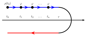
Figure 1: Illustration of the causality-property eq. 8: An $n$/point function $\Gamma^{(n)}_{\tau}$ derived from eq. 5, with all $t_{1},\dots,t_{n}<\tau$, equals the fully dressed $n$/point function. Here, the upper (blue) branch, referred to as $\mathcal{C}^{+}$, encodes time-ordered time evolution, and the lower (red) branch, referred to as $\mathcal{C}^{-}$, encodes anti–time-ordered evolution. The density matrix at the initial time $t_{0}$ is given by $\rho(t_{0})$, and $\varphi$ is the field operator in the Schrödinger picture.

The causal dynamics of the 1PI correlation functions is encoded by that of the effective action $\Gamma_{\tau}[\phi]$, the Legendre transform of the Schwinger functional $W_{\tau}[J]=\log Z_{\tau}[J]$,

$$\Gamma_{\tau}[\phi]\,\operatorname{\vcentcolon=}\,W_{\tau}[J]\,-\,J\cdot\phi\,-\frac{1}{2}\,\phi\cdot R_{\tau}\cdot\phi\,,$$ (5)

with the short hand notation ${f\cdot g=\int\displaylimits_{\mathcal{C}(x)}f(x)g(x)}$ for the CTP integral. Moeover, $J=J[\phi]$ is the solution of $\delta W_{\tau}/\delta J=\phi$. With the sharp causal regulator (4), all fluctuations beyond the cutoff time $\tau$ are completely suppressed. Hence, $\Gamma_{\tau}[\phi]$ contains all fluctuations up to times $\tau$, and the full dynamics of the quantum theory is obtained in the limit $\tau\rightarrow\infty$. An infinitesimal time step is governed by the temporal flow equation, see Gasenzer and Pawlowski (2008); Gasenzer et al. (2010); Corell et al. (2021),

$$\partial_{\tau}\Gamma_{\tau}[\phi]=\frac{1}{2}\operatorname{Tr\!}\Big{[}G_{\tau}[\phi]\cdot\partial_{\tau}R_{\tau}\Big{]}\,,$$ (6)

with the full field-dependent propagator $G_{\tau}[\phi]$,

$$G_{\tau}[\phi](x,y)= \,\left[\frac{\mathrm{i}}{\Gamma^{(2)}_{\tau}[\phi]+R_{\tau}}\right]\!(x,y)\,.$$ (7)

The propagator in eq. 7 vanishes identically for times $x_{0}>\tau$ or $y_{0}>\tau$ due to the regulator. In eq. 7 we used the notation $\Gamma^{(n)}$ for $nth$ derivatives of the effective action w.r.t. $\phi$. We emphasise that the mathematically sound definition of the flow eq. 6 requires the careful evaluation of the regularisation limit of the product of singular distributions $G_{\tau}$ and $\partial_{\tau}R_{\tau}$. This has been discussed in detail in Gasenzer and Pawlowski (2008); Gasenzer et al. (2010) and in particular in Corell et al. (2021); Heller (2021). It leads to a technically straightforward implementation in terms of a modified product of distributions, which we call the $*$-product, see Appendix B. This facilitates in particular the derivation of analytically integrated flows considered later in Section IV.

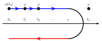
Figure 2: Illustration of the causality-property eq. 9: An $n$/point function $\Gamma^{(n)}_{\tau}$ derived from eq. 5, with at least one time $t_{n}$ larger than $\tau$, remains at its initial value. $\varphi$ at $t_{n}$ can not be placed on the contour, which is best discussed in terms of the sources in (3). A derivative with respect to $J(t_{n}>\tau)$ leads to correlation functions involving $\varphi(t_{n})$ with vanishing measure due to the causal regulator eq. 4. Hence, the 1PI correlation functions remain at their initial values.

The unique causality properties of the t-fRG are best illustrated at the example of the $n$-point correlation functions $\Gamma^{(n)}_{\tau}(x_{1},\dots,x_{n})$. For times $t_{1}\leq t_{2}\leq\cdots\leq t_{n}\leq\tau$ with $t_{i}=x^{0}_{i}$, the $\tau$-dependent correlation function agrees with the full correlation function,

$$\Gamma^{(n)}_{\tau}(x_{1},\dots,x_{n})=\Gamma^{(n)}(x_{1},\dots,x_{n})\,,$$ (8)

where $\Gamma^{(n)}(x_{1},\dots,x_{n}):=\Gamma^{(n)}_{\tau=\infty}(x_{1},\dots,x_{n})$. This situation is depicted in Figure 1. Note that in the absence of field insertions, the contributions from the time evolution operators on the upper part $\mathcal{C}^{+}$ of the Keldysh contour are cancelled by the contributions from the lower part $\mathcal{C}^{-}$. For this reason the extension of the Keldysh contour beyond $x^{0}_{n}$ does not matter, and the flow for $\tau>t_{n}$ does not change the respective $\Gamma^{(n)}_{\tau}$ with $t_{n}<\tau$.

In turn, if at least one time is larger than the cutoff time, that is $t_{n}>\tau$, we have,

$$\Gamma^{(n)}_{\tau}(x_{1},\dots,x_{n})=\Gamma^{(n)}_{t_{0}}(x_{1},\dots,x_{n})\,.$$ (9)

Equation 9 originates from the fact, that the causal regulator $R_{\tau}$ suppresses all fluctuations for times later than $\tau$. This situation is depicted in Figure 2. The fact that the field $\varphi$ at $t_{n}$ can not be placed on the contour, is best interpreted in terms of the sources in eq. 3: sources with times larger than $\tau$ are completely suppressed by the causal regulator. Hence, a derivative with respect to such a source vanishes. In turn, the 1PI correlation functions simply keep their initial values.

Let us emphasise that the properties eq. 8 and eq. 9 are derived from the flow eq. 6. The only additional assumption needed is that the classical vertices are diagonal in time which encodes the locality of the microscopic interactions.

The causality properties eq. 8 and eq. 9 lead to an important identity unique to the present causal t-fRG-approach,

$$\partial_{\tau}G_{\tau}[\operatorname{\hskip 1.00006pt\bar{\phi}\hskip 1.00006pt}]=\mathrm{i}\,(G_{\tau}\partial_{\tau}R_{\tau}G_{\tau})[\operatorname{\hskip 1.00006pt\bar{\phi}\hskip 1.00006pt}]\,,$$ (10)

for a detailed discussion see Corell et al. (2021). Here, $\operatorname{\hskip 1.00006pt\bar{\phi}\hskip 1.00006pt}$ is the physical, in general space-time dependent, background which is given by $\phi^{+}=\operatorname{\hskip 1.00006pt\bar{\phi}\hskip 1.00006pt}=\phi^{-}$ where $\phi^{\pm}$ are the fields on $\mathcal{C}^{\pm}$. Notably, the term involving $\partial_{\tau}\Gamma^{(2)}_{\tau}[\operatorname{\hskip 1.00006pt\bar{\phi}\hskip 1.00006pt}]$ is absent for the causal temporal flow. This remarkable fact is deeply rooted in the locality and causality of the employed regulator, and is also linked to functional optimisation of the fRG Pawlowski (2007). The above properties of local causal flows also imply

$$G_{\tau}[\bar{\phi}](x,y)=G_{\tau=\infty}[\bar{\phi}](x,y)\theta(\tau-x^{0})\theta(\tau-y^{0})\,.$$ (11)

Equation 11 entails that $G_{\tau}[\bar{\phi}]$ is either the fully dressed propagator or it vanishes. This concludes our brief overview on the t-fRG approach.

III The Flow of the Energy-Momentum Tensor

In the present Section we derive the flow of the energy-momentum tensor (EMT), following the derivation in Pawlowski and Wink . We consider a real scalar theory with microscopic three- and four-point interactions, but the derivations trivially generalise to generic quantum field theories. The classical action of the real scalar theory is given by

$$S[\varphi]=\int_{\mathcal{C}}\bigg{\{} \frac{1}{2}\,\partial^{\rho}\varphi(x)\partial_{\rho}\varphi(x)-\frac{m^{2}}{2}\,\varphi(x)^{2}$$

$$- \frac{\lambda_{3}}{3!}\,\varphi(x)^{3}-\frac{\lambda_{4}}{4!}\,\varphi(x)^{4}\bigg{\}}\,.$$ (12)

For the derivation of the EMT we augment eq. 12 with a background metric $g_{\mu\nu}$ with $\int_{\mathcal{C}}\rightarrow\int_{\mathcal{C}}\sqrt{-g(x)}$. The EMT is the metric derivative of the action, evaluated at the flat Minkowski background, $g_{\mu\nu}=\eta_{\mu\nu}$,

$$T_{\mu\nu}(x)=\left.\frac{2}{\sqrt{-g(x)}}\frac{\delta}{\delta g^{\mu\nu}(x)}S[\varphi,g]\right|_{g^{\mu\nu}=\eta^{\mu\nu}}\,.$$ (13)

Here, $g=\det g_{\mu\nu}$ is the determinant of the metric. For the action eq. 12 we are led to,

$$T_{\mu\nu}(x)= \,\partial_{\mu}\varphi\hskip 1.00006pt\partial_{\nu}\varphi$$

$$-\eta_{\mu\nu}\Big{[}\frac{1}{2}\partial^{\rho}\varphi\hskip 1.00006pt\partial_{\rho}\varphi-\frac{m^{2}}{2}\varphi^{2}-\frac{\lambda_{3}}{3!}\varphi^{3}-\frac{\lambda_{4}}{4!}\varphi^{4}\bigg{]}\;.$$ (14)

For some details on metric-derivatives see App. A.

III.1 The General Flow of the EMT

The definition eq. 13 straightforwardly generalises to the regulated effective action $\Gamma_{\tau}$, and the quantum EMT is given by

$$\mathcal{T}_{\mu\nu,\tau}[\phi](x)=\left.\frac{2}{\sqrt{-g(x)}}\frac{\delta}{\delta g^{\mu\nu}(x)}\Gamma_{\tau}[\phi,g]\right|_{g^{\mu\nu}=\eta^{\mu\nu}}\,,$$ (15)

which is related to the expectation value of the classical EMT, $\langle T_{\mu\nu}\rangle$. Importantly, additional terms stem from the renormalisation of the path integral and provide the scale anomaly. Following Pawlowski and Wink , we derive the flow of the EMT as the $\tau$-derivative of eq. 15,

$$\partial_{\tau}\mathcal{T}_{\mu\nu,\tau}(x)=\frac{1}{\sqrt{-g(x)}}\frac{\delta}{\delta g^{\mu\nu}(x)}\Bigl{(}\operatorname{Tr\!}\,G_{\tau}\cdot\dot{R}_{\tau}\Bigr{)}\,,$$ (16)

with $\partial_{\tau}R_{\tau}=\dot{R}_{\tau}$ and $g_{\mu\nu}\to\eta_{\mu\nu}$. For deriving eq. 16 we have commuted metric and $\tau$-derivatives. Since the flow of $\Gamma_{\tau}$ is local and causal, the flow of the EMT inherits these important properties. The trace in eq. 16 is performed with basis functions that are normalised with $1/\sqrt{-g}$, providing a covariant basis.

We proceed with computing the metric-derivative in eq. 16. The derivative of the trace can be evaluated according to eq. 37 and more details can be found in App. A. For the propagator we find

$$\frac{\delta G_{\tau,ab}}{\delta g^{\mu\nu}(x)}= \,\mathrm{i}\left[G_{\tau}\cdot\,\frac{\delta(\Gamma^{(2)}_{\tau}+R_{\tau})}{\delta g^{\mu\nu}(x)}\cdot\,G_{\tau}\right]_{ab}$$

$$+\frac{1}{2}\,g_{\mu\nu}(x)\big{[}G_{\tau,ax}{}_{bx}+G_{\tau,bx}{}_{ax}\big{]}\,.$$ (17)

Here, we use a shorthand notation denoting space-time arguments as indices. The first term on the right-hand side originates from its inverse relation to $\Gamma^{(2)}_{\tau}$, cf. eq. 7. The second term comes from the covariant definition of the inverse in line with the present covariant basis, leading to $G\cdot G^{-1}=\one$, and is defined in eq. 38. Note that the operator product on the left-hand side also contains a factor of $\sqrt{-g}$. These appearances of the metric are hit by the metric-derivative and produce the second term in eq. 17. Notably, this term cancels with the metric derivative of the trace in eq. 16. Finally, we arrive at

$$\partial_{\tau}\mathcal{T}_{\mu\nu,\tau}(x)=\operatorname{Tr\!}\Bigg{[}G_{\tau}\cdot\frac{1}{\sqrt{-g(x)}}\frac{\delta\dot{R}_{\tau}}{\delta g^{\mu\nu}(x)}\Bigg{]}$$

$$+\mathrm{i}\operatorname{Tr\!}\Bigg{[}\big{(}G_{\tau}\cdot\dot{R}_{\tau}\cdot G_{\tau}\hskip 1.00006pt\big{)}\cdot\frac{1}{\sqrt{-g(x)}}\frac{\delta\big{(}\Gamma^{(2)}_{\tau}+R_{\tau}\big{)}}{\delta g^{\mu\nu}(x)}\Bigg{]}\,,$$ (18)

with $g^{\mu\nu}\rightarrow\eta^{\mu\nu}$. We emphasise that the above derivation holds true for general regulators, and in particular for standard momentum space regulators, see Pawlowski and Wink .

III.2 Causal Temporal Flow of the EMT

Next, we turn to the causal structure of the temporal flow. We shall see that this causal structure leads us to a novel, unique result: The regulator terms in eq. 18 drop out completely in contradistinction to momentum space regulators used in Pawlowski and Wink . This is due to the fact that the causal regulator, as opposed all other regulators, does not introduce violations of scale invariance. This fact and its implications with regard to the trace anomaly of the EMT are discussed in more detail in Section III.3.

For proving the absence of regulator terms in the causal temporal flow of the EMT we first use eq. 10, only valid for the present sharp temporal regulator. This identity allows us to combine the regulator terms in eq. 18 into a total $\tau$-derivative,

$$G_{\tau}\cdot\frac{1}{\sqrt{-g(x)}}\frac{\delta\dot{R}_{\tau}}{\delta g^{\mu\nu}(x)}+\dot{G}_{\tau}\cdot\frac{1}{\sqrt{-g(x)}}\frac{\delta R_{\tau}}{\delta g^{\mu\nu}(x)}$$

$$=\frac{1}{2}g_{\mu\nu}(x)\,\partial_{\tau}\big{(}G_{\tau}\cdot R_{\tau}\big{)}\,,$$ (19)

where we have suppressed the field dependences in $G_{\tau}$. In the first line of eq. 19 we have used (41): both, $R_{\tau}$ and $\partial_{\tau}R_{\tau}$ are proportional to the covariant unity, defined in eq. 38, and hence their metric derivative is proportional to $R_{\tau}$ and $\partial_{\tau}R_{\tau}$ respectively with the same (metric) prefactors. Now we use that

$$\Bigl{(}R_{\tau}\cdot G_{\tau}\Bigr{)}[\operatorname{\hskip 1.00006pt\bar{\phi}\hskip 1.00006pt}](x,y)=\left\{\begin{aligned} 0\phantom{\operatorname{\delta_{\mathcal{C}}}_{\!,xy}}\quad\text{if}\,x^{0}\leq\tau\\ \phantom{0}\operatorname{\delta_{\mathcal{C}}}_{\!,xy}\hskip 1.00006pt\hskip 1.00006pt\quad\text{if}\,x^{0}>\tau\end{aligned}\right.\,.$$ (20)

where we have assumed $x^{0}>y^{0}$. This follows straightforwardly from the local causal properties of the temporal regulator eq. 4, see Heller (2021) for more details. Its $\tau$-derivative and the trace leaves us with a constant theory-independent term which we simply drop.

Then, we arrive at the remarkable fact that the metric-derivatives of the causal regulator do not contribute to the temporal flow of the EMT, which now reads

$$\partial_{\tau}\mathcal{T}_{\mu\nu,\tau}[\operatorname{\hskip 1.00006pt\bar{\phi}\hskip 1.00006pt}](x)=\frac{\mathrm{i}}{2}\Bigl{[}\operatorname{Tr\!}\,(G_{\tau}\cdot\dot{R}_{\tau}\cdot G_{\tau})\cdot\mathcal{T}^{(2)}_{\mu\nu,\tau}\Bigr{]}[\operatorname{\hskip 1.00006pt\bar{\phi}\hskip 1.00006pt}](x),$$ (21)

with

$$\mathcal{T}^{(2)}_{\mu\nu,\tau}[\phi](x,y,z)=\frac{2}{\sqrt{-g(x)}}\frac{\delta\Gamma^{(2)}_{\tau}[\phi](y,z)}{\delta g^{\mu\nu}(x)}\,,$$ (22)

Equation 21 has the standard form of the flow of composite operators derived in Pawlowski (2007), see also Pagani (2016) and the review Dupuis et al. (2021). It does not hold for momentum space regulators that introduce a (further) breaking of scale symmetry, see also Morris and Percacci (2019).

Using again the key identity eq. 10, only valid for the present local causal regulator, we are led to

$$\partial_{\tau}\mathcal{T}_{\mu\nu,\tau}[\operatorname{\hskip 1.00006pt\bar{\phi}\hskip 1.00006pt}](x)=\frac{1}{2}\Bigl{[}\operatorname{Tr\!}\,\partial_{\tau}G_{\tau}\cdot\mathcal{T}^{(2)}_{\mu\nu,\tau}\Bigr{]}[\operatorname{\hskip 1.00006pt\bar{\phi}\hskip 1.00006pt}](x),$$ (23)

our final concise form of the EMT-flow. Equation 23 is also straightforwardly generalised to EMT-correlations.

III.3 Properties of the causal temporal EMT-flow

As already mentioned above, eq. 21 is the standard flow equation for composite operators. This equation does not hold true for the flow of the EMT for general regulators, given by eq. 18. Indeed, for momentum space regulators the terms in eq. 18 that originate from the metric dependence of the regulator generate (part of) the scale or trace anomaly. This can be understood as follows: For an infrared momentum space cutoff the theory tends towards the classical one in the ultraviolet as all momentum fluctuations are suppressed. For classical scale invariant theory, the trace of the classical EMT $T^{\textrm{cl}}$ vanishes as does $T^{\textrm{cl},(2)}{}_{\mu}{}^{\mu}$. If the full EMT at the initial time $t_{0}$ is identified with the classical EMT, $\mathcal{T}_{\mu\nu,t_{0}}[\operatorname{\hskip 1.00006pt\bar{\phi}\hskip 1.00006pt}](x)=T_{\mu\nu}^{\textrm{cl}}[\operatorname{\hskip 1.00006pt\bar{\phi}\hskip 1.00006pt}](x)$, the flow in eq. 21 vanishes identically. However, the quantisation procedure typically breaks scale invariance due to the necessity of renormalisation, leading to a quantum scale anomaly. For an infrared regulator the quantisation of momentum modes and the respective scale anomaly is carried by the regulator and its metric dependence. Thus the flow successively generates the part of the scale anomaly generated by the quantum fluctuations of the respective momentum shells. In turn, the part of the scale anomaly carried by ultraviolet momentum modes larger than the initial infrared cutoff scale has to be present in the initial condition.

The causal temporal flow of this work does not implement a momentum cutoff and the initial condition is the full renormalised quantum theory at hand at the initial time $t_{0}$. Specifically, the unitary quantum dynamics described by the causal temporal flow does not alter the UV properties of the theory. Thus, if we use renormalised initial conditions, the flow of the EMT is given by eq. 21. This will be discussed in more details in Corell et al. , see also Corell et al. (2021); Corell (2021); Heller (2021). We also remark that for some applications we may augment the present temporal cutoff with an additional spatial momentum cutoff. Then, the spatial momentum regularisation leads to a combined momentum and temporal flow of the EMT of the form eq. 18.

Next, we comment briefly on the use of the flow of the EMT eq. 21 for monitoring or guaranteeing energy conservation in generic t-fRG truncations. For instance, we can use the flow of the EMT to close a truncation: while part of the flow of correlation functions present in a given truncation is derived from the flow of the effective action, the flow of the remaining set of correlation functions is derived from the flow of the EMT. This guarantees the unitarity of the flow of the EMT. Complementarily, the (integrated) flow of the EMT can be used numerically to correct for potential violations of energy conservation.

We also remark that a suitable generalisation of the procedure as in Garbrecht and Millington (2016) offers an attractive option. The general idea would be to alleviate potential violations of energy conservation caused by the truncation by using a suitably constructed background $\bar{\phi}$. Finally, the flow of the EMT in eq. 21 can be used to simply monitor the conservation laws in supposedly unitary approximations.

IV Integrated Causal Flow of the Energy-Momentum Tensor

Here, we discuss the analytic integration of the causal temporal flow of the EMT. This analytic integration is only possible due to the local and causal structure of the t-fRG approach leading to the simple flow eq. 23. Due to the causality-properties discussed in Section II, the only non-vanishing contributions to the integrated flow appear if the external time $x^{0}$ is equal to $\tau$. This results in

$$\int_{t_{0}}^{\infty}\operatorname{d\!}\tau\;\mathcal{T}^{(2)}_{\mu\nu,\tau}[\operatorname{\hskip 1.00006pt\bar{\phi}\hskip 1.00006pt}](x)\,\cdot\,\partial_{\tau}G_{\tau}[\operatorname{\hskip 1.00006pt\bar{\phi}\hskip 1.00006pt}]=\mathcal{T}^{(2)}_{\mu\nu}[\operatorname{\hskip 1.00006pt\bar{\phi}\hskip 1.00006pt}](x)\,*\,G[\operatorname{\hskip 1.00006pt\bar{\phi}\hskip 1.00006pt}]\,,$$ (24)

with the $*$-product detailed in Appendix B. It accounts for the well-defined product of causal singular distributions, see also Corell et al. (2021); Heller (2021). Note also that the causality-properties eq. 8 and eq. 9 lead to causal constraints on the temporal flows of general operators. For instance, the causal constraint on the flow of the EMT is given by

$$\partial_{\tau}\mathcal{T}_{\mu\nu,\tau}[\operatorname{\hskip 1.00006pt\bar{\phi}\hskip 1.00006pt}](x)\propto\delta(\tau-x^{0})*\theta(\tau-x^{0})\,.$$ (25)

Importantly, the flow is only non-vanishing for $\tau=x^{0}$. This entails that the $\tau$-integral in eq. 24 terminates at $\tau=x^{0}+\xi$ with $\xi\to 0$, as the only contribution to the causal temporal flow of the EMT is proportional to $\delta(\tau-x^{0})*\theta(\tau-x^{0})$.

These types of constraints lead to the remarkable fact that the causal temporal flow can be integrated analytically. For the correlation functions themselves, this led to a novel one-loop exact functional relation for quantum field theories, see Corell et al. (2021); Corell (2021); Heller (2021). Here we also arrive at a one-loop ecact relation for the integrated flow of the EMT, in comparison to the three-loop exact Dyson-Schwinger equation (DSE) for the EMT. The latter property originates in the fact that the EMT is a composite operator with up to forth order powers in the field, as we shall see later in Section V.

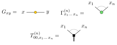
Figure 3: Symbols used in the graphical representation of the diagrams contributing to $\langle T_{00}[\varphi](x)\rangle$, cf. eq. 30 and Figure 4. The black line with the orange circle represents the fully dressed field-dependent propagator $G_{xy}[\phi]=\mathrm{i}\big{[}\Gamma^{(2)}[\phi]\big{]}_{xy}^{-1}$. The green circle with $n$ lines attached to it denotes the fully dressed $n$-point vertex $\Gamma^{(n)}_{x_{1}\dots\,x_{n}}[\phi]$. The black square with $n$ lines attached to it denotes the $n$th $\phi$/derivative of the classical energy $T^{(n)}_{00}[\phi](x,x_{1}\dots\,x_{n})$, where the double line indicates the dependence on the external argument $x$.

With the $*$/product, see Appendix B, we express the integrated flow of the EMT as

$$\mathcal{T}_{\mu\nu}(x)-\mathcal{T}_{\mu\nu,\mathrm{init}}(x)=\frac{1}{2}\operatorname{Tr\!}\Big{[}\mathcal{T}^{(2)}_{\mu\nu}(x)\,*\,G\Big{]}\,.$$ (26)

In eq. 26 we have suppressed the dependence on the background $\bar{\phi}$. By $\mathcal{T}_{\mu\nu,\mathrm{init}}(x)$, we denote the EMT at the initial time $\tau=t_{0}$. As the causal temporal flow does not introduce a quantum violation of scale invariance, the respective anomalous terms cancel in the difference.

For the solution of eq. 26 we note that structurally it is very similar to a Dyson-Schwinger equation, for recent reviews see e.g. Fischer (2019); Huber (2020). In particular, eq. 26 is a functional integral equation. Accordingly, it can be solved using the iteration techniques as used for DSEs: on the right hand side of (26) we insert an appropriate guess for the solution, for instance the initial condition $\mathcal{T}_{\mu\nu,\mathrm{init}}(x)$. Then, we iterate eq. 26 until convergence. For this procedure it is useful to express the EMT and its derivatives, $\mathcal{T}^{(n)}$, in terms of the initial condition $\mathcal{T}^{(n)}_{\mathrm{init}}$ and the deviation $\Delta\mathcal{T}^{(n)}_{\tau}$. For instance, the second derivative reads

$$\mathcal{T}^{(2)}_{\mu\nu,\tau}(x,a,b)\,=\,\mathcal{T}^{(2)}_{\mu\nu,\mathrm{init}}(x,a,b)\,+\,\Delta\mathcal{T}^{(2)}_{\mu\nu,\tau}(x,a,b)\,,$$ (27)

for general $\tau$. It has been shown in Corell et al. (2021); Corell (2021); Heller (2021), that the causal constraints of the temporal flow allow us to classify the non-vanishing contributions to the flow according to the space-time structure of the interactions. Moreover, generically the local contributions dominate the flow. Accordingly, we define

$$\Delta\mathcal{T}^{(2)}_{\mu\nu,\tau}(x,a,b)= \,\Delta\mathcal{T}^{(2)}_{\mu\nu,\mathrm{local}\,\tau}(x,a,b)$$

$$+\Delta\mathcal{T}^{(2)}_{\mu\nu,\mathrm{nl}}(x,a,b)\,\theta(\tau-x^{0})\theta(\tau-a^{0})\theta(\tau-b^{0})\,.$$ (28)

Here, all contributions containing $\operatorname{\delta_{\mathcal{C}}}$-functions are contained in $\Delta\mathcal{T}^{(2)}_{\mu\nu,\mathrm{local}\,\tau}$. Inserting eq. 28 in eq. 26, we notice that $\Delta\mathcal{T}^{(2)}_{\mu\nu,\mathrm{nl}}$ in the second line of eq. 28 does not satisfy the causal constraint of the EMT, eq. 25. Hence it does not contribute to the integrated flow, and the only contribution stems from the local term in eq. 28.

V Integrated Flow and diagrammatic representations of the EMT

Figure 4: Diagrammatic representation of the EMT, eq. 30, using the diagrammatic depiction of propagators and vertices in Figure 4, and dropping any reference to the renormalisation. We refer to the diagram involving $G^{3}$ as the sunset. The diagram involving $G^{2}$ is called the eight. The diagram involving $G^{4}$ and $\Gamma^{(3)}$ is called the squint-sunset. The diagram with $G^{4}$ and $\Gamma^{(4)}$ is called the basketball.

The integrated flow eq. 26 constitutes another important result of the present work and offers a surprisingly simple diagrammatic form of the full energy-momentum tensor of the quantum field theory at hand. In the present Section we show how it can be used to recover the standard diagrammatic representation of the EMT in terms of its DSE. This derivation also shows the power of the analytical one-loop representation with the $*$-product.

For this purpose we focus on the energy $\mathcal{T}_{00}$. For the present real scalar theory with the action eq. 12, the $00$-component of the classical EMT is read-off from eq. 14,

$$T_{00}[\varphi](x)=\frac{1}{2}\Big{[}\big{(}\partial_{x^{0}}\varphi\big{)}^{2}+\big{(}\partial_{\mathbf{x}}\varphi\big{)}^{2}+m^{2}\varphi^{2}\Big{]}+\frac{\lambda_{3}}{3!}\varphi^{3}+\frac{\lambda_{4}}{4!}\varphi^{4}\,.$$ (29)

The expectation values of powers of fields can be rewritten in terms of propagators and higher order correlation functions with eq. 43. This leads us to

$$\mathcal{T}_{00}[\phi](x)= T^{\textrm{(ren)}}_{00}[\phi](x)+\Biggl{[}\frac{1}{2}\,T_{00}^{(2)}[\phi](x)\cdot G+\frac{\mathrm{i}}{6}\,T_{00}^{(3)}[\phi](x)\cdot G^{3}\cdot\Gamma^{(3)}$$

$$+\frac{1}{8}\,T_{00}^{(4)}[\phi](x)\cdot G^{2}-\frac{1}{8}\,T_{00}^{(4)}[\phi](x)\cdot G^{4}\cdot\Gamma^{(3)}\cdot G\cdot\Gamma^{(3)}+\frac{\mathrm{i}}{24}\,T_{00}^{(4)}[\phi](x)\cdot G^{4}\cdot\Gamma^{(4)}\Biggr{]}_{\textrm{ren}}\,,$$ (30)

with $\phi$-dependent vertices $T_{00}^{(n)}[\phi](x)\operatorname{\vcentcolon=}\delta T_{00}[\phi](x)/\delta\phi^{n}$. These vertices can be expanded in powers of the fields. For example, the second term in eq. 30 reads

$$\frac{1}{2}\,T_{00}^{(2)}[\phi](x)\cdot G= \frac{1}{2}\lim_{y\to x}\partial_{x}\partial_{y}G_{xy}+\frac{1}{2}m^{2}G_{xx}$$

$$+\frac{1}{2}\,\lambda_{3}\phi_{x}G_{xx}+\frac{1}{4}\,\lambda_{4}\phi^{2}_{x}G_{xx}\,,$$ (31)

where we used $\langle(\partial_{x}\varphi_{x})(\partial_{x}\varphi_{x})\rangle=\lim_{y\rightarrow x}\partial_{x}\partial_{y}\langle\varphi_{x}\varphi_{y}\rangle$. Moreover, the third term in the first line of eq. 30 is proportional to $T_{00}^{(3)}[\phi]=\lambda_{3}+\lambda_{4}\phi$.

We note that eq. 30 is a formal expression as the diagrams require renormalisation, depending on the dimension $D$ of the theory. Moreover, part of the derivative terms in $T_{\mu\nu}$ come from the Lagrangian part proportional to $\eta_{\mu\nu}$ and renormalise accordingly. In turn, the other part comes from the composite operator $\partial_{\mu}\phi\,\partial_{\nu}\phi$ with its own renormalisation. It is indeed this difference which accounts for the trace anomaly and hence the breaking of quantum scale invariance. In the present work we are interested in the structural aspects of temporal flows, the renormalisation intricacies are discussed elsewhere in Corell et al. . We indicate the respective anomalous terms with the superscript (ren) in $T^{\textrm{(ren)}}_{00}$ and the renormalisation of the diagrams with the respective subscript of the square bracket. In particular, summing over all diagonal components we have $T^{\textrm{(ren)}}{}_{\mu}{}^{\mu}=T_{\mu}{}^{\mu}+{\cal A}$ with the trace anomaly ${\cal A}$.

Similar derivations also hold for all components $T_{\mu\nu}$ of the EMT, which leaves us with a closed three-loop exact expression for the quantum EMT. Equation 30 is depicted graphically in Figure 4, using Figure 3. Its different graphs constitute different topologies in a diagrammatic expansion: Apart from the one-loop contribution we have a diagram with $G^{2}$ (eight), a diagram with $G^{3}$ (sunset), a diagram with $G^{4}$ and $\Gamma^{(3)}$ (squint-sunset), and a diagram with $G^{4}$ and $\Gamma^{(4)}$ (basketball).

The integrated flow has to reproduce these different topologies as well as the respective prefactors. For identifying the relevant contributions of eq. 30 to $\mathcal{T}^{(2)}_{00}$, we use the integrated flow eq. 26 and the causal constraint eq. 25: only terms that generate at least one $\operatorname{\delta_{\mathcal{C}}}$ can contribute to the integrated flow. Thus, none of the field-derivatives of the terms in the second line in eq. 30 have to be considered (the second line in Figure 4). From the sunset, only the contribution involving the explicit field dependence gives rise to a $\operatorname{\delta_{\mathcal{C}}}$. Thus, the relevant local contributions to $\mathcal{T}^{(2)}_{00}$ are contained in

$$\mathcal{T}^{(2)}_{00,\mathrm{local}}(x,a,b)=T^{(2)}_{00}(x,a,b)+\Delta\mathcal{T}^{(2)}_{00,\mathrm{local}}(x,a,b)\,,$$ (32)

where we again have dropped the reference to the necessary renormalisation. The $\phi$-derivatives of the kinetic term for $G$ are also non-local while the other two terms in eq. 31 generate local contributions. In summary, we obtain

$$\Delta\mathcal{T}^{(2)}_{00,\mathrm{local}}(x,a,b)= \,\frac{\mathrm{i}}{2}\left[\lambda_{3}G^{2}_{x}\Gamma^{(3)}_{a}\hskip 1.00006pt\operatorname{\delta_{\mathcal{C}}}_{\!,xb}+(a\leftrightarrow b)\right]+\frac{\mathrm{i}}{2}\left[\lambda_{4}\phi_{x}\,G^{2}_{x}\Gamma^{(3)}_{a}\hskip 1.00006pt\operatorname{\delta_{\mathcal{C}}}_{\!,xb}+(a\leftrightarrow b)\right]$$

$$\,+\frac{1}{2}\,\lambda_{4}G_{xx}\operatorname{\delta_{\mathcal{C}}}_{\!xa}\operatorname{\delta_{\mathcal{C}}}_{\!xb}+\frac{\mathrm{i}}{6}\left[\lambda_{4}G^{3}_{x}\Gamma^{(4)}_{a}\hskip 1.00006pt\operatorname{\delta_{\mathcal{C}}}_{\!,xb}+\,(a\leftrightarrow b)\right]-\frac{1}{2}\left[\lambda_{4}G^{3}_{x}\Gamma^{(3)}_{a}G\Gamma^{(3)}\hskip 1.00006pt\operatorname{\delta_{\mathcal{C}}}_{\!,xb}+\,(a\leftrightarrow b)\right]\,.$$ (33)

For a concise representation we have used a short hand notation $[G^{m}_{x}F]$, where the dependence on any internal space-time indices has been dropped, see Appendix D. The first term in eq. 33 is generated from $\phi_{x}G_{xx}$. The second and the third term are generated from $\phi_{x}^{2}G_{xx}$. The last two terms are generated by the relevant part of the sunset. For all these terms, at least one field must be hit by the $\phi$-derivative to generate a local contribution. Now we insert eq. 32 into the integrated flow eq. 26. The arguments $a,b$ of all terms in eq. 32 get closed by the $\tau$-derivative of the propagator, $\partial_{\tau}G_{\tau,ab}$. In terms of loop topology we observe that closing the first two terms in eq. 33 with $G_{ab}$ gives rise to the sunset. The remaining terms generate the eight, the basketball and the squint-sunset. In conclusion all topologies are present.

diagram	$G\,*\,\Delta\mathcal{T}^{(2)}_{00,\mathrm{local}}$	factor
eight	$\partial_{\tau}G_{\tau,ab}\;G_{\tau,xx}\operatorname{\delta_{\mathcal{C}}}_{\!,xa}\operatorname{\delta_{\mathcal{C}}}_{\!,xb}$	$\nicefrac{{2}}{{4}}$
sunset	$\big{[}\hskip 1.00006pt\partial_{\tau}G_{\tau,ab}\;G^{2}_{\tau,x}\operatorname{\delta_{\mathcal{C}}}_{\!,x(a\leftrightarrow b)}\Gamma^{(3)}_{\tau,a}\hskip 1.00006pt\big{]}$	$\nicefrac{{2}}{{3}}$
basketball	$\big{[}\hskip 1.00006pt\partial_{\tau}G_{\tau,ab}\;G^{3}_{\tau,x}\operatorname{\delta_{\mathcal{C}}}_{\!,x(a\leftrightarrow b)}\Gamma^{(4)}_{\tau,a}\hskip 1.00006pt\big{]}$	$\nicefrac{{2}}{{4}}$
squint-sunset	$\big{[}\hskip 1.00006pt\partial_{\tau}G_{\tau,ab}\;G^{3}_{\tau,x}\operatorname{\delta_{\mathcal{C}}}_{\!,x(a\leftrightarrow b)}\Gamma^{(3)}_{\tau,a}G_{\tau}\Gamma^{(3)}_{\tau}\hskip 1.00006pt\big{]}$	$\nicefrac{{2}}{{4}}$

Table 1: Factors due to the evaluation of the $*$-product for the respective diagrams. The $*$-product was defined in eq. 42. Here, we use the following shorthand notation: $[\dots\operatorname{\delta_{\mathcal{C}}}_{\!,x(a\leftrightarrow b)}\dots]=[\dots\operatorname{\delta_{\mathcal{C}}}_{\!,xb}\dots]+[\dots\operatorname{\delta_{\mathcal{C}}}_{\!,xa}\dots]$, cf. eq. 33.

It remains to compute the combinatoric factors. To that end we first note that the $*$-product in $T^{(2)}_{00}[\operatorname{\hskip 1.00006pt\bar{\phi}\hskip 1.00006pt}](x)*G_{ab}[\operatorname{\hskip 1.00006pt\bar{\phi}\hskip 1.00006pt}]$ reduces to the standard one, $T^{(2)}_{00}[\operatorname{\hskip 1.00006pt\bar{\phi}\hskip 1.00006pt}](x)\cdot G$, since $\operatorname{\hskip 1.00006pt\bar{\phi}\hskip 1.00006pt}_{x}$ does not give rise to any $\theta_{\tau x}$. For the remaining diagrams of $\Delta\mathcal{T}^{(2)}_{00,\mathrm{local}}$, the $*$-product has to be evaluated. The corresponding contributions from the $*$-product can be found in Table 1, and are derived by using App. B. Combining the factors of Table 1 with the ones already present in eq. 33 and the overall factor of $\nicefrac{{1}}{{2}}$ of the flow, cf. eq. 26, the integrated flow of the EMT reads

$$\mathcal{T}_{00}[\operatorname{\hskip 1.00006pt\bar{\phi}\hskip 1.00006pt}](x)-\mathcal{T}_{00,\mathrm{init}}[\operatorname{\hskip 1.00006pt\bar{\phi}\hskip 1.00006pt}](x)= \frac{1}{2}\,T_{00}^{(2)}[\phi](x)\cdot G+\frac{\mathrm{i}}{6}\,T_{00}^{(3)}[\phi](x)\cdot G^{3}\cdot\Gamma^{(3)}$$

$$+\frac{1}{8}\,T_{00}^{(4)}[\phi](x)\cdot G^{2}-\frac{1}{8}\,T_{00}^{(4)}[\phi](x)\cdot G^{4}\cdot\Gamma^{(3)}\cdot G\cdot\Gamma^{(3)}+\frac{\mathrm{i}}{24}\,T_{00}^{(4)}[\phi](x)\cdot G^{4}\cdot\Gamma^{(4)}\,.$$ (34)

Thus, we already reproduced all diagrams of eq. 30 with their correct prefactors. Note also that the difference on the left-hand side eliminates the anomalous contributions that sum up to the trace anomaly. The latter is not time-dependent and hence does not change in the temporal flow. This implies, that the right-hand side of eq. 30 also does not encode the anomalous terms. What is left is to determine $\mathcal{T}_{00,\mathrm{init}}[\operatorname{\hskip 1.00006pt\bar{\phi}\hskip 1.00006pt}](x)=\mathcal{T}_{00,\tau=t_{0}}[\operatorname{\hskip 1.00006pt\bar{\phi}\hskip 1.00006pt}](x)$, where we restrict ourselves to times $x^{0}>t_{0}$. For these times the initial $\mathcal{T}_{00,\mathrm{init}}$ does not comprise any fluctuations due to the causal regulator and it reduces to $T^{(\textrm{ren})}_{00}[\operatorname{\hskip 1.00006pt\bar{\phi}\hskip 1.00006pt}](x)$ including the trace anomaly. In summary, we fully recover the diagrammatic representation eq. 30 from the integrated flow. Moreover, eq. 34 readily extends to all components of the EMT. Finally, as for the EMT-flow eq. 23, the derivations above straightforwardly extend to $n$-point correlations $\langle T_{\mu_{1}\nu_{1}}\cdots T_{\mu_{n}\nu_{n}}\rangle$ of the EMT. Specifically, components of the two-point correlation functions are chiefly important for the derivation of transport coefficients.

Equation 34 is a non-trivial demonstration of the consistency of the t-fRG formalism as well as the computational simplicity of its unique one-loop exact representation: The integrated one-loop exact causal temporal flow of the EMT encodes the full diagrammatic representation eq. 30 of the expectation value of the EMT. Moreover, this section also demonstrates the power of the causal constraints inherent to the t-fRG. These constraints greatly simplified the above derivation as the number of relevant diagrammatic contributions was reduced dramatically. Importantly, the $*$-products, that encode the full causal structure of the flows, have a practical usability within numerical applications.

VI Conclusion

We have derived the flow of the energy-momentum tensor for general regulators. This equation contains terms that describe the explicit breaking of scale invariance by general regulators. We have shown, that for the causal temporal regulator these terms are absent since this regulator simply ensures a causal time evolution, and does not trigger any violation of scale invariance. Consequently, a potential trace anomaly of the EMT is described by providing renormalised initial conditions for the causal temporal flow. Alternatively one can augment the temporal regulator with a standard spatial infrared momentum regulator. Then the trace anomaly is generated by the spatial momentum flow.

We have integrated the causal flow of the energy-momentum tensor analytically, which leads us to a one-loop excact functional relation for the energy-momentum tensor. With the help of a product of singular distributions put forward in Corell et al. (2021) this relation can be also implemented numerically. We have also demonstrated explicitly that it is consistent with the usual Dyson-Schwinger equation of the expectation value of the energy-momentum tensor.

Appendix A Useful Identities for Metric-Derivatives

Here, we display some useful identities involving the metric-derivative. For the derivative of the metric and its determinant, we use the standard identities

$$\frac{\delta g^{\alpha\beta}(a)}{\delta g^{\mu\nu}(b)} =\Big{(}\delta^{\alpha}_{\mu}\delta^{\beta}_{\nu}+\delta^{\alpha}_{\nu}\delta^{\beta}_{\mu}\Big{)}\operatorname{\delta_{\mathcal{C}}}(a-b)$$ (35)

$$\frac{\delta\sqrt{-g(a)}}{g^{\mu\nu}(b)} =\,-\frac{1}{2}\,\sqrt{-g(a)}\,g_{\mu\nu}(a)\operatorname{\delta_{\mathcal{C}}}(a-b)\,.$$ (36)

Using these two relations, it is straightforward to derive

$$\frac{\delta}{\delta g^{\mu\nu}(b)}\left[\int_{\mathcal{C},a}\!\!\!\!\!\sqrt{-g(a)}\right]=-\frac{1}{2}\int_{\mathcal{C},a}\!\!\!\!\!\sqrt{-g(a)}\,g_{\mu\nu}(a)\operatorname{\delta_{\mathcal{C}}}(a-b)\,.$$ (37)

The manifestly covariant $\delta$-function is defined by

$${}_{ab}=\frac{1}{\sqrt{-g(a)}}\operatorname{\delta_{\mathcal{C}}}(a-b)$$ (38)

Accordingly, its metric-derivative reads

$$\frac{\delta\,{}_{ab}}{\delta g^{\mu\nu}(x)} =\frac{\delta}{\delta g^{\mu\nu}(x)}\left(\frac{\operatorname{\delta_{\mathcal{C}}}(a-b)}{\sqrt{-g(a)}}\right)$$

$$=\,\frac{1}{2}\,g_{\mu\nu}(a)\operatorname{\delta_{\mathcal{C}}}(a-x)\,{}_{ab}\;.$$ (39)

These relations ensure that

$$\frac{\delta}{\delta g^{\mu\nu}(x)}\bigg{(}\int_{\mathcal{C}}\sqrt{-g}\;\one\bigg{)}=0\,.$$ (40)

In Section III.2, we need the metric-derivative of the regulator $R_{\tau}$ and that of $\partial_{\tau}R_{\tau}$. Both are proportional to and have no further metric dependence. Hence, we find with eq. 39,

$$\frac{1}{\sqrt{-g(x)}}\frac{\delta(R_{\tau}\,,\,\partial_{\tau}R_{\tau})_{ab}}{\delta g^{\mu\nu}(x)}=\frac{1}{2}g_{\mu\nu}(x)\,(R_{\tau}\,,\,\partial_{\tau}R_{\tau})_{ab}{}_{ax}\,,$$ (41)

where no sum over the index $a$ is implied.

Appendix B The $*$-product

The $*$-product accounts for the fact that the regulator, the propagator and the other correlators can have coincident singularities Corell et al. (2021); Heller (2021), leading to contributions of the form $\delta(\tau-x^{0})\,*\,\theta(\tau-x^{0})$. These singularities have to be treated with care. To that end, we introduce a regularisation $\varepsilon$ for the distributions present. Then, such products lead to, e.g. Corell et al. (2021),

$$\delta_{\tau x}\,*\,\theta_{\tau x}^{n}\;\operatorname{\vcentcolon=}\;\lim_{\varepsilon\to 0}\,\delta_{\varepsilon,\tau x}\,[\theta_{\varepsilon,\tau x}]^{n}\,,$$ (42a)

with

$$\lim_{\varepsilon\to 0}\,\delta_{\varepsilon,\tau x}\,[\theta_{\varepsilon,\tau x}]^{n}=\delta_{\tau x}\,\int_{0}^{1}dx\,x^{n}=\frac{1}{n+1}\;\delta_{\tau x}\,.$$ (42b)

Here, $\theta_{\varepsilon,\tau x}\operatorname{\vcentcolon=}\theta_{\varepsilon}(\tau-x^{0})$ and similarly for the $\delta$/distribution. Crucially, the $\delta$- and $\theta$-functions in eq. 42 share the same regularisation $\varepsilon$ as distributions. This is due to the fact that this regularisation is inherited from the regularisation of the sharp cutoff, $R_{\tau}\rightarrow R_{\varepsilon,\tau}$. Thus, the product of distributions that come from different $n$-point functions is uniquely defined in terms of eq. 42. We remark that identities like eq. 42 have also been used in momentum space fRGs, see e.g. Morris (1994); Metzner et al. (2012).

Appendix C Expectation Values

For the computation of the expectation value of the classical energy eq. 29, cf. eq. 30 and Figure 4 respectively, we use the functional relation (see e.g. Pawlowski (2007)),

$$\left\langle\prod_{i=1}^{n}\varphi(x_{i})\right\rangle=\prod_{i=1}^{n}\left[\int\displaylimits_{\mathrlap{\mathcal{C},z_{i}}}G[\phi](x_{i},z_{i})\frac{\delta}{\delta\phi(z_{i})}+\phi(x_{i})\right]\,.$$ (43)

Appendix D Shorthand Notation for Loops

Consider a product of $m$ propagators in a diagram, given by $G_{x1}\cdots G_{xm}$ and fully contracted with another tensor $F_{1\dots m}$, to wit,

$$[G^{m}_{x}F]=G_{x1}\cdots G_{xm}F_{1\dots m}\,,$$ (44)

and $F_{1\dots m}$ comprises the rest of the diagram. For instance,

$$[G^{2}_{x}\Gamma^{(3)}_{a}\hskip 1.00006pt\operatorname{\delta_{\mathcal{C}}}_{\!,xb}]=G_{xz_{1}}G_{xz_{2}}\,\Gamma^{(3)}_{az_{1}z_{2}}\hskip 1.00006pt\operatorname{\delta_{\mathcal{C}}}_{\!,xb}\,,$$ (45)

where sums or integrals over the indices $z_{1},z_{2}$ are implied.

References

- Gasenzer and Pawlowski (2008) T. Gasenzer and J. M. Pawlowski, Phys. Lett. B 670, 135 (2008), arXiv:0710.4627 [cond-mat.other] .
- Gasenzer et al. (2010) T. Gasenzer, S. Kessler, and J. M. Pawlowski, Eur. Phys. J. C 70, 423 (2010), arXiv:1003.4163 [cond-mat.quant-gas] .
- Corell et al. (2021) L. Corell, A. K. Cyrol, M. Heller, and J. M. Pawlowski, Phys. Rev. D 104, 025005 (2021), arXiv:1910.09369 [hep-th] .
- Schwinger (1961) J. S. Schwinger, J. Math. Phys. 2, 407 (1961).
- Keldysh (1964) L. V. Keldysh, Zh. Eksp. Teor. Fiz. 47, 1515 (1964), [English translation: JETP 20, 1018 (1965)].
- Calzetta and Hu (2008) E. A. Calzetta and B.-L. B. Hu, Nonequilibrium Quantum Field Theory, Cambridge Monographs on Mathematical Physics (Cambridge University Press, 2008).
- Stefanucci and Van Leeuwen (2013) G. Stefanucci and R. Van Leeuwen, Nonequilibrium Many-Body Theory Quantum Syst. A Mod. Introd. (Cambridge Univ. Press, 2013).
- Berges (2015) J. Berges, (2015), arXiv:1503.02907 [hep-ph] .
- Berges and Hoffmeister (2009) J. Berges and G. Hoffmeister, Nucl. Phys. B 813, 383 (2009), arXiv:0809.5208 [hep-th] .
- Huelsmann et al. (2020) S. Huelsmann, S. Schlichting, and P. Scior, Phys. Rev. D 102, 096004 (2020), arXiv:2009.04194 .
- Tan et al. (2021) Y.-y. Tan, Y.-r. Chen, and W.-j. Fu, (2021), arXiv:2107.06482 [hep-ph] .
- Dupuis et al. (2021) N. Dupuis, L. Canet, A. Eichhorn, W. Metzner, J. M. Pawlowski, M. Tissier, and N. Wschebor, Phys. Rept. 910, 1 (2021), arXiv:2006.04853 [cond-mat.stat-mech] .
- Heller (2021) M. Heller, Ph.D. thesis, Heidelberg University (2021).
- Pawlowski (2007) J. M. Pawlowski, Annals Phys. 322, 2831 (2007), arXiv:hep-th/0512261 .
- (15) J. M. Pawlowski and N. Wink, In preparation.
- Pagani (2016) C. Pagani, Phys. Rev. D 94, 045001 (2016), arXiv:1603.07250 [hep-th] .
- Morris and Percacci (2019) T. R. Morris and R. Percacci, Phys. Rev. D 99, 105007 (2019), arXiv:1810.09824 [hep-th] .
- (18) L. Corell, M. Heller, and J. M. Pawlowski, In preparation.
- Corell (2021) L. Corell, Ph.D. thesis, Heidelberg University (2021).
- Garbrecht and Millington (2016) B. Garbrecht and P. Millington, Nucl. Phys. B 906, 105 (2016), arXiv:1509.07847 [hep-th] .
- Fischer (2019) C. S. Fischer, Prog. Part. Nucl. Phys. 105, 1 (2019), arXiv:1810.12938 [hep-ph] .
- Huber (2020) M. Q. Huber, Phys. Rept. 879, 1 (2020), arXiv:1808.05227 [hep-ph] .
- Morris (1994) T. R. Morris, Int. J. Mod. Phys. A 9, 2411 (1994), arXiv:hep-ph/9308265 .
- Metzner et al. (2012) W. Metzner, M. Salmhofer, C. Honerkamp, V. Meden, and K. Schonhammer, Rev. Mod. Phys. 84, 299 (2012), arXiv:1105.5289 [cond-mat.str-el] .