Quantum lower and upper speed limits

Abstract

We derive generalized quantum speed limit inequalities that represent limitations on the time evolution of quantum states. They are extensions of the original inequality and are applied to the overlap between the time-evolved state and an arbitrary state. We can discuss the lower limit of the overlap, in addition to the upper limit as in the original inequality, which allows us to estimate the minimum time for the evolution toward a target state. The inequalities are written by using an arbitrary reference state and are flexibly used to obtain a tight bound. We demonstrate these properties by using the twisted Landau–Zener model, the Grover Hamiltonian, and a periodically-oscillating Hamiltonian.

1 Introduction

The quantum speed limit is an inequality that is applied to a distance measure of quantum states. In the Mandelstam–Tamm relation [1, 2, 3, 4] the distance measure is bounded from above by the energy dispersion. In the Margolus–Levitin relation [5], it is bounded by the average energy. The inequalities are interpreted as time-energy uncertainty relations and are closely related to the geometric structure of Hilbert space.

The original inequalities applied to quantum pure states can be generalized to other problems such as quantum mixed states with dissipative environments and probability distributions in classical stochastic processes [6, 7, 8, 9, 10, 11]. Different forms of the speed limit are obtained in different situations, but they are written by the corresponding metric and can be treated in a unified way. They are applied to various problems including quantum control, quantum computing, information processing, and stochastic thermodynamics. We can find many applications in literature [12].

Although the inequality is applied to a broad range of systems, it gives a loose bound in most of realistic systems. The bound usually goes to infinity when we consider a large processing time or a large system size.

A different type of quantum speed limit was discussed in recent studies. The standard limit is applied to the overlap between the time-evolved state and the initial state. An inequality was derived for the overlap between the time-evolved state and the adiabatic state in [13] and between different time-evolved states in [14]. Some applications of the method can be found in [15, 16]. These results imply that the time evolution of a quantum state is characterized in multiple ways by using various reference states. In this paper, we pursue this problem and derive quantum speed limit inequalities satisfied among three quantum states. The result is a generalization of the original Mandelstam–Tamm relation and can be applicable to any quantum states.

This paper is organized as follows. In section 2, we derive our main result, the quantum upper and lower speed limits. We study several examples in the following sections. We treat the twisted Landau–Zener model in section 3, the Grover Hamiltonian in section 4, and a periodically-oscillating Hamiltonian in section 5. The result is summarized in section 6.

2 Speed limits from triangle inequality

We consider quantum states described by the density operator $\hat{\rho}$. Different quantum states are distinguished by introducing a distance measure $D(\hat{\rho}_{1},\hat{\rho}_{2})$. Its properties are prescribed by the standard requirements: nonnegativity, symmetry, and triangle inequality

$$D(\hat{\rho}_{1},\hat{\rho}_{2})\leq D(\hat{\rho}_{2},\hat{\rho}_{3})+D(\hat{\rho}_{3},\hat{\rho}_{1}).$$ (1)

It is well-known that the trace distance and the fidelity satisfy the requirements and are used in many applications [17]. In the present paper, we mainly use the fidelity

$$\Theta(\hat{\rho}_{1},\hat{\rho}_{2})=\arccos{\rm Tr}\,\left(\hat{\rho}_{1}^{1/2}\hat{\rho}_{2}\hat{\rho}_{1}^{1/2}\right)^{1/2}.$$ (2)

When the system is described by the pure state $\hat{\rho}=|\psi\rangle\langle\psi|$, the fidelity is written by the state overlap

$$\Theta_{\psi_{1},\psi_{2}}=\arccos|\langle\psi_{1}|\psi_{2}\rangle|.$$ (3)

Then, the triangle inequality reads

$$|\Theta_{\psi_{1}\psi_{3}}-\Theta_{\psi_{2},\psi_{3}}|\leq\Theta_{\psi_{1},\psi_{2}}\leq\Theta_{\psi_{1},\psi_{3}}+\Theta_{\psi_{2},\psi_{3}}.$$ (4)

We can use this inequality to find a lower limit and a upper limit for $\Theta_{\psi_{1},\psi_{2}}$. The triangle inequality among three quantum states was used to derive a novel type of speed limit [18, 19]. Here, we derive different limits by using the method in [13, 14].

In most of the applications, we are interested in the fidelity between the time-evolved state $|\psi(t)\rangle$ and a target state $|\psi_{\rm target}\rangle$. The former state is obtained from the Schrödinger equation $i\partial_{t}|\psi(t)\rangle=\hat{H}(t)|\psi(t)\rangle$ with the Hamiltonian $\hat{H}(t)$. We also introduce a reference state $|\psi_{\rm ref}(t)\rangle$ to write the relation

$$\Theta_{\psi_{\rm target},\psi_{\rm ref}(t)}-\Theta_{\psi_{\rm ref}(t),\psi(t)}\leq\Theta_{\psi_{\rm target},\psi(t)}\leq\Theta_{\psi_{\rm target},\psi_{\rm ref}(t)}+\Theta_{\psi_{\rm ref}(t),\psi(t)}.$$ (5)

In the standard quantum speed limit inequality, the fidelity $\Theta_{\psi(0),\psi(t)}$ is bounded from above as $\Theta_{\psi(0),\psi(t)}\leq\int_{0}^{t}\rmd t^{\prime}\sigma[\hat{H}(t^{\prime}),\psi(t^{\prime})]$ where $\sigma[\hat{H},\psi]=(\langle\psi|\hat{H}^{2}|\psi\rangle-\langle\psi|\hat{H}|\psi\rangle^{2})^{1/2}$. The main idea of the present paper is to use the inequality for the fidelity $\Theta_{\psi_{\rm ref}(t),\psi(t)}$ developed in [13, 14]. To apply the standard Mandelstam–Tamm relation, we introduce the Hermitian operator $\hat{H}_{\rm ref}(t)$ from the relation $i\partial_{t}|\psi_{\rm ref}(t)\rangle=\hat{H}_{\rm ref}(t)|\psi_{\rm ref}(t)\rangle$ with $|\psi_{\rm ref}(0)\rangle=|\psi(0)\rangle$. We write the overlap $\langle\psi_{\rm ref}(t)|\psi(t)\rangle$ as $\langle\psi(0)|\tilde{\psi}(t)\rangle$ where $|\tilde{\psi}(t)\rangle$ satisfies the Schrödinger equation with an effective Hamiltonian comprised of $\hat{H}(t)$ and $\hat{H}_{\rm ref}(t)$ [13, 14]. Then, we obtain

$$\Theta_{\rm l}\leq\Theta_{\psi_{\rm target},\psi(t)}\leq\Theta_{\rm u},$$ (6)

where

$$\Theta_{\rm l}=\Theta_{\psi_{\rm target},\psi_{\rm ref}(t)}-\int_{0}^{t}\rmd t^{\prime}\,\sigma[\hat{H}(t^{\prime})-\hat{H}_{\rm ref}(t^{\prime}),\psi_{\rm ref}(t^{\prime})],$$ (7)

$$\Theta_{\rm u}=\Theta_{\psi_{\rm target},\psi_{\rm ref}(t)}+\int_{0}^{t}\rmd t^{\prime}\,\sigma[\hat{H}(t^{\prime})-\hat{H}_{\rm ref}(t^{\prime}),\psi_{\rm ref}(t^{\prime})].$$ (8)

This is the main result of the present paper.

The main advantage of the relation in equation (6) is that the inequalities hold for arbitrary choices of a target state $|\psi_{\rm target}\rangle$ and a reference state $|\psi_{\rm ref}(t)\rangle$. By using the reference state $|\psi_{\rm ref}(t)\rangle$, we can derive a lower limit of $\Theta_{\psi_{\rm target},\psi(t)}$ in addition to the upper limit. The bounds can be estimated without knowing the time-evolved state $|\psi(t)\rangle$.

We note that the inequalities also hold when we use $|\psi(t^{\prime})\rangle$ in place of $|\psi_{\rm ref}(t^{\prime})\rangle$ for the variance $\sigma$ [13]. The standard upper speed limit is obtained by setting $|\psi_{\rm target}\rangle=|\psi(0)\rangle$, $\hat{H}_{\rm ref}(t)=0$, and $\sigma[\hat{H}(t^{\prime})-\hat{H}_{\rm ref}(t^{\prime}),\psi_{\rm ref}(t^{\prime})]\to\sigma[\hat{H}(t^{\prime}),\psi(t^{\prime})]$.

Since the fidelity distance satisfies $0\leq\Theta\leq\pi/2$, the bound is useful only when it is within the domain of definition. When we choose $|\psi_{\rm target}\rangle=|\psi(0)\rangle$, $\Theta_{\psi(0),\psi(t)}$ is upper-bounded for a short period of time and we can discuss how fast the time-evolved state deviates from the initial state. This gives a result similar to the standard speed limit. By choosing the reference state in a proper way, we can obtain a tight bound. On the other hand, when the state evolves toward a target state $|\psi_{\rm target}\rangle$ with $\langle\psi_{\rm target}|\psi(0)\rangle=0$, we can estimate a minimum time $t$ for the time-evolved state $|\psi(t)\rangle$ to reach the target state as $|\langle\psi_{\rm target}|\psi(t)\rangle|=1$.

There are several ways to utilize the bounds. In the following sections, we discuss possible applications by using several model Hamiltonians.

3 Twisted Landau–Zener model: tight bound at large time

When we exactly know the state evolution $|\psi_{\rm ref}(t)\rangle$ under the Hamiltonian $\hat{H}_{\rm ref}(t)$, we can estimate the bound on the unknown state $|\psi(t)\rangle$ under the Hamiltonian $\hat{H}(t)$. Since the bound is represented by the time integration of the variance $\sigma$, the bound becomes tight when $\sigma$ takes nonzero values only for a finite interval of $t$.

We study these properties by using the twisted Landau–Zener Hamiltonian [20]

$$\hat{H}(t)=\left(\begin{array}[]{cc}vt&\Delta\rme^{-i\varphi(t)}\\ \Delta\rme^{i\varphi(t)}&-vt\end{array}\right).$$ (11)

$\Delta$ and $v$ are arbitrary positive parameters and $\varphi(t)$ represents an arbitrary function of $t$. This Hamiltonian is compared to the standard form of the Landau–Zener Hamiltonian [21, 22]

$$\hat{H}_{\rm ref}(t)=\left(\begin{array}[]{cc}vt&\Delta\\ \Delta&-vt\end{array}\right).$$ (14)

We start the time evolution from

$$|\psi(-\infty)\rangle=\left(\begin{array}[]{c}1\\ 0\end{array}\right),$$ (17)

and study the overlap $\langle\psi_{\rm target}|\psi(\infty)\rangle$ where $|\psi_{\rm target}\rangle=|\psi(-\infty)\rangle$. $|\psi_{\rm ref}(t)\rangle$ is exactly solvable and we obtain the Landau–Zener formula

$$|\langle\psi_{\rm target}|\psi_{\rm ref}(\infty)\rangle|=\exp\left(-\frac{\pi\Delta^{2}}{2v}\right).$$ (18)

The twisted Landau–Zener model is equivalent to the Landau–Zener model with a nonlinear protocol. It is shown by using the transformation to the rotating frame as

$$\exp\left[\frac{i}{2}\varphi(t)\left(\begin{array}[]{cc}1&0\\ 0&-1\end{array}\right)\right]\left(\hat{H}(t)-i\partial_{t}\right)\exp\left[-\frac{i}{2}\varphi(t)\left(\begin{array}[]{cc}1&0\\ 0&-1\end{array}\right)\right]$$ (23)

$$= \left(\begin{array}[]{cc}vt-\frac{1}{2}\dot{\varphi}(t)&\Delta\\ \Delta&-\left(vt-\frac{1}{2}\dot{\varphi}(t)\right)\end{array}\right),$$ (26)

where the dot symbol denotes the time derivative. It is difficult to obtain the general solution for a given $\varphi(t)$ and we apply the inequalities derived in the previous section.

With the use of the reference Hamiltonian in equation (14), the bounds of $\Theta_{\psi_{\rm target},\psi(\infty)}$ in the twisted Landau–Zener model are written as

$$\Theta_{\rm u,l}=\arccos\exp\left(-\frac{\pi\Delta^{2}}{2v}\right)\pm\int_{0}^{\infty}\rmd t\,\sigma(\hat{H}(t)-\hat{H}_{\rm ref}(t),\psi_{\rm ref}(t)).$$ (27)

Using the relation $\sigma(\hat{X},\psi_{\rm ref})\leq\sqrt{\langle\psi_{\rm ref}|\hat{X}^{2}|\psi_{\rm ref}\rangle}$, we can estimate the second term without knowing $|\psi_{\rm ref}(t)\rangle$ as

$$\int_{0}^{\infty}\rmd t\,\sigma(\hat{H}(t)-\hat{H}_{\rm ref}(t),\psi_{\rm ref}(t))\leq 2\Delta\int_{0}^{\infty}\rmd t\,\left|\sin\frac{\varphi(t)}{2}\right|.$$ (28)

To obtain a finite value of the bounds, we require that $\varphi(t)$ (mod $2\pi$) is nonzero for a finite domain of $t$. We choose two types of the protocol:

$$\varphi(t)=\left\{\begin{array}[]{ll}\pi\left(1+\tanh\frac{t}{\tau}\right)&\mbox{protocol 1}\\ \pi\exp\left(-\frac{t^{2}}{\tau^{2}}\right)&\mbox{protocol 2}\end{array}\right..$$ (31)

We plot the parameter dependence of $\Theta_{\psi_{\rm target},\psi(\infty)}$ in figure 1. We can find finite bounds even at the limit $t\to\infty$. We note that the standard quantum speed limit does not give any meaningful result since the bound goes to infinity.

We also plot results for various choices of parameters in figure 2. The result shows that the bounds become tight for small $\tau$ and large $v$. The former condition, small $\tau$, is reasonable since $\sigma$ becomes small in that limit. The latter condition represents nonadiabatic regime. The opposite limit, small $v$, is basically described by the adiabatic approximation. Our inequalities can be useful in the nonadiabatic regime rather than in the adiabatic one.

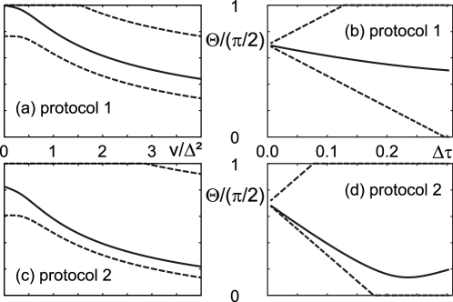
Figure 1: Quantum speed limit in the twisted Landau–Zener model. $\Theta_{\psi_{\rm target},\psi(\infty)}$ (solid line) and $\Theta_{\rm u,l}$ (dashed lines) are plotted as a function of parameters $\Delta\tau$ and $v/\Delta^{2}$. Each panel shows the result with the protocol 1 and $\Delta\tau=0.1$ (a), with the protocol 1 and $v/\Delta^{2}=2.0$ (b), with the protocol 2 and $\Delta\tau=0.1$ (c), and with the protocol 2 and $v/\Delta^{2}=2.0$ (d).

Figure 2: $(\Theta_{\rm u},\Theta_{\psi_{\rm target},\psi(\infty)})$ (blue cross) and $(\Theta_{\rm u},\Theta_{\psi_{\rm target},\psi(\infty)})$ (red slanted cross) in the twisted Landau–Zener model. The parameters are sampled within $0<\Delta\tau\leq 1$ and $0<\frac{v}{\Delta^{2}}\leq 4$.

4 Grover Hamiltonian: protocol-independent bound

As we can see from the example in the previous section, the bound is in principle dependent on the Hamiltonian and on the protocol. In the present section, we discuss that a universal bound is obtained by choosing the reference state in a proper way.

One of the reasonable choice of the reference state is the adiabatic state $|\psi_{\rm ad}(t)\rangle$. It is written by using the instantaneous eigenstates of the Hamiltonian $\hat{H}(t)$. It corresponds to choosing the reference Hamiltonian as the counterdiabatic Hamiltonian $\hat{H}_{\rm ref}(t)=\hat{H}(t)+\hat{H}_{\rm cd}(t)$.

The counterdiabatic driving is used in the method of shortcuts to adiabaticity [23, 24, 25, 26, 27, 28]. When the Hamiltonian is written by the spectral representation as

$$\hat{H}(t)=\sum_{n}\epsilon_{n}(\bm{\lambda}(t))|n(\bm{\lambda}(t))\rangle\langle n(\bm{\lambda}(t))|,$$ (32)

the counterdiabatic term is given by

$$\hat{H}_{\rm cd}(t)=\dot{\bm{\lambda}}(t)\cdot i\sum_{n}\left(1-|n(\bm{\lambda}(t))\rangle\langle n(\bm{\lambda}(t))|\right)|\bm{\nabla}_{\bm{\lambda}}n(\bm{\lambda}(t))\rangle\langle n(\bm{\lambda}(t))|,$$ (33)

where $\bm{\lambda}(t)=(\lambda_{1}(t),\lambda_{2}(t),\dots)$ is a set of time-dependent parameters. The solution of the Schrödinger equation with the Hamiltonian $\hat{H}(t)+\hat{H}_{\rm cd}(t)$ is given by the adiabatic state

$$|\psi_{\rm ad}(t)\rangle = \sum_{n}|n(\bm{\lambda}(t))\rangle\langle n(\bm{\lambda}(0))|\psi(0)\rangle$$ (34)

$$\times\exp\left[-i\int_{0}^{t}\rmd t^{\prime}\epsilon_{n}(\bm{\lambda}(t^{\prime}))-\int_{\bm{\lambda}(0)}^{\bm{\lambda}(t)}\rmd\bm{\lambda}\cdot\langle n(\bm{\lambda})|\bm{\nabla}_{\bm{\lambda}}n(\bm{\lambda})\rangle\right].$$

The counterdiabatic term is written in a form $\hat{H}_{\rm cd}(t)=\dot{\bm{\lambda}}(t)\cdot\bm{A}(\bm{\lambda}(t))$ and the adiabatic gauge potential $\bm{A}(\bm{\lambda})$ characterizes the geometric property of the system.

We set $|\psi_{\rm ref}(t)\rangle=|\psi_{\rm ad}(t)\rangle$ to find a universal bound. When we choose the initial state as one of eigenstates of $\hat{H}(0)$, and use a single parameter $\lambda(t)$, the time integration of the variance is written as

$$\int_{0}^{t}\rmd t^{\prime}\sigma(\hat{H}_{\rm cd}(t^{\prime}),\psi_{\rm ad}(t^{\prime}))=\int_{\lambda(0)}^{\lambda(t)}\rmd\lambda\,\sigma_{A}(\lambda),$$ (35)

where $\sigma_{A}(\lambda)$ represents the variance of the adiabatic gauge potential $A$ with respect to the eigenstate. This representation means that the bounds are dependent only on the initial and final values of the protocol. When $\bm{\lambda}(t)$ has multiple components, the time integration of the variance depends only on the path in parameter space $\bm{\lambda}$ and is independent of the velocities on the path.

To demonstrate the described general properties, we study the Grover Hamiltonian [29, 30, 31]

$$\hat{H}(t)=A(t)\left(1-|+\rangle\langle+|\right)+B(t)\left(1-|0\rangle\langle 0|\right).$$ (36)

We want to select the target state $|\psi_{\rm target}\rangle=|0\rangle$ from among a set of states $\{|i\rangle\}_{i=0,1,\dots,N-1}$. The initial state is chosen as

$$|+\rangle=\frac{1}{\sqrt{N}}\sum_{i=0}^{N-1}|i\rangle,$$ (37)

and the Hamiltonian changes from $\hat{H}(0)=1-|+\rangle\langle+|$ to $\hat{H}(t_{\rm f})=1-|0\rangle\langle 0|$. In the adiabatic quantum computation, the Hamiltonian is changed slowly and the system goes from the initial state to the target state $|0\rangle$.

The counterdiabatic Hamiltonian is written as

$$\hat{H}_{\rm cd}(t)=\frac{i}{2}\sqrt{\frac{N}{N-1}}\dot{\theta}(t)\left(|0\rangle\langle+|-|+\rangle\langle 0|\right),$$ (38)

where

$$\theta(t)=\arctan\frac{\frac{\sqrt{N-1}}{N}A(t)}{\frac{1}{2}\left[\left(1-\frac{2}{N}\right)A(t)-B(t)\right]}.$$ (39)

For $\Theta(t)=\arccos|\langle 0|\psi(t)\rangle|$, the bounds are calculated as

$$\Theta_{\rm u}(t)=\frac{\pi-\theta(0)}{2},$$ (40)

$$\Theta_{\rm l}(t)=\frac{\pi-\theta(0)}{2}-(\theta(t)-\theta(0)).$$ (41)

The upper bound is time independent, which shows that $\Theta$ does not exceed the initial value. The lower bound shows that we can find the minimum time for the time-evolved state to reach the target state. The minimum time $t_{\rm min}$ is obtained by solving $\theta(t_{\rm min})=(\pi+\theta(0))/2$.

As a typical choice of the protocol in the adiabatic quantum computation, we use $A(t)=A(0)(1-s(t/t_{\rm f}))$ and $B(t)=A(0)s(t/t_{\rm f})$ [32]. The function $s(\tau)$ is an increasing function satisfying $s(0)=0$ and $s(1)=1$. We choose two types of the protocol as

$$s(\tau)=\left\{\begin{array}[]{ll}\displaystyle\frac{1-\rme^{-k\tau}}{(1-\rme^{-k/2})(1+\rme^{-k(\tau-1/2)})}&\mbox{protocol 1}\\ \displaystyle\frac{1}{k}\ln\frac{(\rme^{k/2}-1)\tau+1}{1-(1-\rme^{-k/2})\tau}&\mbox{protocol 2}\end{array}\right.,$$ (44)

where $k\geq 1$. In both cases, $s(\tau)\sim\tau$ for $k=1$. This linear protocol is frequently used in the adiabatic quantum computation. As we increase $k$, $s(\tau)$ changes rapidly and the adiabaticity condition is broken. We plot the protocol 1 in the left panel of figure 3 and the protocol 2 in the left panel of figure 4.

The results are shown in the right panel of figure 3 for the protocol 1 and of figure 4 for the protocol 2. In the present choice of parameters $N=10$ and $A(0)t_{\rm f}=20$, $\Theta$ is well described by the adiabatic approximation for small $k$ and shows a nonadiabatic behavior for large $k$. When $k$ is a large value for the protocol 2, the result is rapidly oscillating and the amplitude of the oscillation is tightly bounded by $\Theta_{\rm u,l}$. This result shows that $\Theta_{\rm u,l}$ are not overestimation and give reasonable bounds. As in the result of the previous section, the quantum speed limit is useful when we consider nonadiabatic regime.

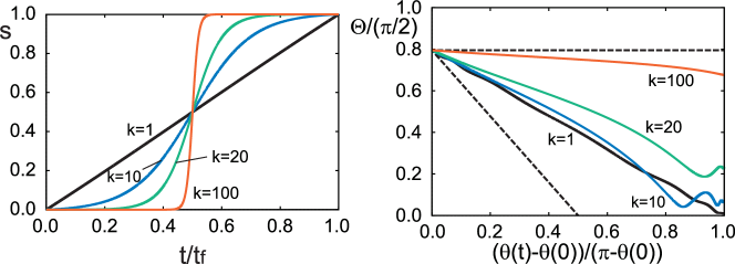
Figure 3: Quantum speed limit of the Grover Hamiltonian with $N=10$, $A(0)t_{\rm f}=20$, and the protocol 1 in the left panel. The right panel represents $\Theta$ (solid lines) and $\Theta_{\rm u,l}$ (dashed lines).

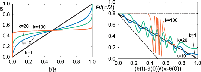
Figure 4: Quantum speed limit of the Grover Hamiltonian with $N=10$, $A(0)t_{\rm f}=20$, and the protocol 2 in the left panel. The right panel represents $\Theta$ (solid lines) and $\Theta_{\rm u,l}$ (dashed lines).

5 Periodically-oscillating system: bound optimization

The third example treats a periodically-oscillating Hamiltonian $\hat{H}(t)$. Generally speaking, the standard quantum speed limit bound becomes loose when the Hamiltonian changes back and forth. We discuss how this problem is improved by using a proper reference state.

As a reference Hamiltonian, we use a time-independent Hamiltonian $\hat{H}_{\rm ref}$. This choice allows us to evaluate the bound easily. When $\hat{H}(t)$ changes rapidly, we can obtain the effective time-independent Hamiltonian from the Floquet–Magnus expansion [33, 34]. The effective Hamiltonian can be utilized as a reference one.

To obtain a tractable result, we use the exactly-solvable Hamiltonian

$$\hat{H}(t)=\frac{1}{2}\left(\begin{array}[]{cc}\Delta&h\rme^{-i\omega t}\\ h\rme^{i\omega t}&-\Delta\end{array}\right),$$ (47)

where $\Delta$, $h$, $\omega$ are positive parameters. When $\omega$ is small, the adiabatic approximation gives a reasonable result and the opposite limit, large $\omega$, is described by the Floquet–Magnus expansion. Here, we consider the large $\omega$ case. The Floquet–Magnus expansion gives a time-independent Hamiltonian

$$\hat{H}_{\rm ref}=\frac{1}{2}\left(\begin{array}[]{cc}\Delta_{\rm ref}&h_{\rm ref}\\ h_{\rm ref}&-\Delta_{\rm ref}\end{array}\right).$$ (50)

Up to the second order in $1/\omega$, we obtain

$$\Delta_{\rm ref}=\Delta-\frac{h^{2}}{2\omega}-\frac{\Delta h^{2}}{\omega^{2}},$$ (51)

$$h_{\rm ref}=-\frac{\Delta h}{\omega}-\frac{\Delta^{2}h}{\omega^{2}}+\frac{h^{3}}{2\omega^{2}}.$$ (52)

The reference state is obtained as $|\psi_{\rm ref}(t)\rangle=\rme^{-i\hat{H}_{\rm ref}t}|\psi(0)\rangle$.

We start the time evolution from the eigenstate of the Hamiltonian $\hat{H}(0)$ with the positive eigenvalue. When we choose the initial state as the target state $|\psi_{\rm target}\rangle=|\psi(0)\rangle$, $\Theta(t)=\arccos|\langle\psi(0)|\psi(t)\rangle|$ changes from the initial value $\Theta(0)=0$ as we show crossed points in the panels (a) and (c) of figure 5. In this case, the lower bound $\Theta_{\rm l}(t)$ (lower dashed line) is calculated to give negative values at any $t$ and we cannot obtain a useful result. On the other hand, the upper bound $\Theta_{\rm l}(t)$ (upper dashed line) gives a reasonable result which is smaller than the bound obtained in the standard quantum speed limit (dotted line).

The negative lower bound is due to the choice of the target state. In the panels (b) and (d) of figure 5, we show the result in the case of the target state

$$|\psi_{\rm target}\rangle=\frac{1}{\sqrt{2}}\left(\begin{array}[]{c}1\\ i\end{array}\right).$$ (55)

In this case, the lower and upper bounds are between $0$ and $\pi/2$ at not too large $t$.

The use of the Floquet–Magnus expansion does not necessarily give a tight bound. Although the reference state $|\psi_{\rm ref}(t)\rangle$ gives a good approximation to the time-evolved state $|\psi(t)\rangle$, the variance $\sigma$ is not necessarily optimized. We choose the reference Hamiltonian in equation (50) and the parameters $\Delta_{\rm ref}$ and $h_{\rm ref}$ are optimized so that $\Theta_{\rm u}$ is minimized and $\Theta_{\rm l}$ is maximized at each $t$. The result is shown by the solid lines in figure 5. The bounds are useful at transient times, several periods of the oscillation. It is remarkable to notice that, in the panels (a) and (c), the lower bound gives a positive value at a small $t$.

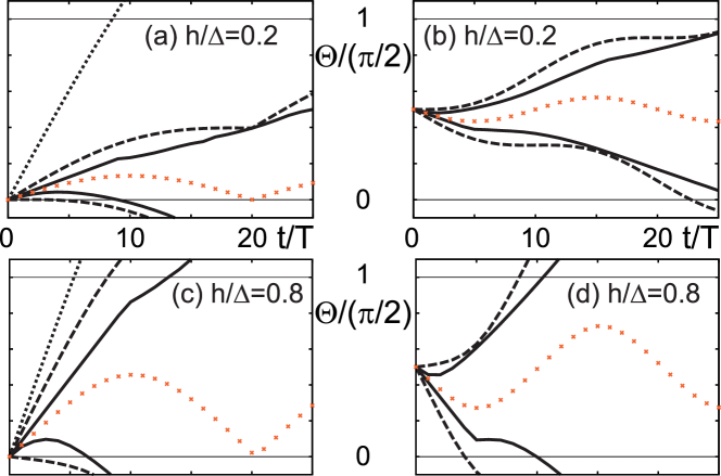
Figure 5: Quantum speed limit of the periodically-oscillating Hamiltonian in equation (47). $\Theta$ (points) is plotted as a function of $t$ at each panel. $T=2\pi/\omega$ represents the period of the oscillation and we take $\omega/\Delta=20$. The parameter $h/\Delta$ is $0.2$ for the panel (a) and (b) and $0.8$ for (c) and (d). We use $|\psi_{\rm target}\rangle=|\psi(0)\rangle$ for the panel (a) and (c), and equation (55) for (b) and (d). The bounds are estimated by three ways. The standard quantum speed limit is represented by the dotted line. The dashed lines represent $\Theta_{\rm u,l}$ in the case that the Floquet state is chosen for the reference state. The solid lines represent $\Theta_{\rm u,l}$ for the optimized reference state.

6 Summary and perspectives

We have discussed lower and upper quantum speed limits. The inequalities are represented by using three quantum states. The choices of the reference state and the target state are arbitrary and we can considerably improve the standard bound.

We stress two important points in deriving the improved inequalities: the triangle inequality in equation (1) and the estimation of the bound by the method in [13, 14]. The triangle inequality is represented by using the density operator and the general distance measure and is generally satisfied without any approximation. Although we have treated pure quantum states in this paper, our method is applicable to broader classes of quantum and classical systems in cases that the distance measure is defined. In open quantum and classical systems, speed limits are derived in some situations, and it would be a straightforward task to apply the method developed in the present paper.

It is also an interesting problem to apply the present method to systems with many degrees of freedom. The system energy is typically proportional to the system size $N$, which implies that the variance $\sigma$ is proportional to $N$. The overlap between two different quantum states $|\psi_{1}\rangle$ and $|\psi_{2}\rangle$ has a form $|\langle\psi_{1}|\psi_{2}\rangle|\sim\rme^{-Ng}$ and the quantum speed limit inequality becomes a trivial relation. Although it is possible to find a bound for the rate function $g=-\frac{1}{N}\ln|\langle\psi_{1}|\psi_{2}\rangle|$ [13], $g$ is not a distance measure and we cannot use the triangle inequality. In spite of this problem, we still have a possibility to find a meaningful result by using arbitrariness on the choice of the reference state. It will be an interesting future problem.

References

References

- [1] Mandelstam L and Tamm I 1945 The uncertainty relation between energy and time in nonrelativistic quantum mechanics J. Phys. (Moscow) 9 249
- [2] Fleming G N 1973 A unitarity bound on the evolution of nonstationary states Nuovo Cimento A 16 232
- [3] Bhattacharyya B 1983 Quantum decay and the Mandelstam–Tamm time–energy inequality J. Phys. A 16 2993
- [4] Vaidman L 1992 Minimum time for the evolution to an orthogonal quantum state Am. J. Phys. 60 182
- [5] Margolus N and Levitin L B 1998 The maximum speed of dynamical evolution Physica D 120 188
- [6] del Campo A, Egusquiza I L, Plenio M B and Huelga S F 2013 Quantum speed limits in open system dynamics Phys. Rev. Lett. 110 050403
- [7] Pires D P, Cianciaruso M, Céleri L C, Adesso G and Soares-Pinto D O 2016 Generalized geometric quantum speed limits Phys. Rev. X 6 021031
- [8] Shanahan B, Chenu A, Margolus N and del Campo A 2018 Quantum speed limits across the quantum-to-classical transition Phys. Rev. Lett. 120 070401
- [9] Okuyama M and Ohzeki M 2018 Quantum speed limit is not quantum Phys. Rev. Lett. 120 070402
- [10] Shiraishi N, Funo K and Saito K 2018 Speed limit for classical stochastic processes Phys. Rev. Lett. 121 070601
- [11] Funo K, Shiraishi N and Saito K 2019 Speed limit for open quantum systems New J. Phys. 21 013006
- [12] Deffner S and Campbell S 2017 Quantum speed limits: from Heisenberg’s uncertainty principle to optimal quantum control J. Phys. A: Math. Theor. 50 453001
- [13] Suzuki K and Takahashi K 2020 Performance evaluation of adiabatic quantum computation via quantum speed limits and possible applications to many-body systems Phys. Rev. Res. 2 032016(R)
- [14] Hatomura T and Takahashi K 2021 Controlling and exploring quantum systems by algebraic expression of adiabatic gauge potential Phys. Rev. A 103 012220
- [15] Funo K, Lambert N and Nori F 2021 General bound on the performance of counter-diabatic driving acting on dissipative spin systems Phys. Rev. Lett. 127 150401
- [16] Hatomura T 2021 Performance evaluation of invariant-based inverse engineering by quantum speed limit arXiv 2112.07253
- [17] Nielsen M A and Chuang I L 2000 Quantum Computation and Quantum Information (Cambridge: Cambridge University Press)
- [18] Lychkovskiy O, Gamayun O and Cheianov V 2017 Time scale for adiabaticity breakdown in driven many-body systems and orthogonality catastrophe Phys. Rev. Lett. 119 200401
- [19] Chen J-H and Cheianov V 2021 Bounds on quantum adiabaticity in driven many-body systems from generalized orthogonality catastrophe and quantum speed limit arXiv: 2112.06900
- [20] Berry M V 1990 Geometric amplitude factors in adiabatic quantum transitions Proc. R. Soc. Lond. A 430 405
- [21] Landau L 1932 Zur Theorie der Energieubertragung II Phys. Sov. Union 2 46
- [22] Zener C 1932 Non-adiabatic crossing of energy levels Proc. Royal Soc. A 137 696
- [23] Demirplak M and Rice S A 2003 Adiabatic population transfer with control fields J. Phys. Chem. A 107 9937
- [24] Demirplak M and Rice S A 2005 Assisted adiabatic passage revisited J. Phys. Chem. B 109 6838
- [25] Berry M V 2009 Transitionless quantum driving J. Phys. A 42 365303
- [26] Chen X, Ruschhaupt A, Schmidt S, del Campo A, Guéry-Odelin D and Muga J G 2010 Fast optimal frictionless atom cooling in harmonic traps: shortcut to adiabaticity Phys. Rev. Lett. 104 063002
- [27] Torrontegui E, Ibáñez S, Martínez-Garaot S, Modugno S, del Campo A, Guéry-Odelin D, Ruschhaupt A, Chen X and Muga J G 2013 Shortcuts to adiabaticity Adv. At. Mol. Opt. Phys. 62 117
- [28] Guéry-Odelin D, Ruschhaupt A, Kiely A, Torrontegui E, Martínez-Garaot S and Muga J G 2019 Shortcuts to adiabaticity: concepts, methods, and applications Rev. Mod. Phys. 91 045001
- [29] Grover L K 1997 Quantum mechanics helps in searching for a needle in a haystack Phys. Rev. Lett. 79 325
- [30] Farhi E and Gutmann S 1998 An analog analogue of a digital quantum computation Phys. Rev. A 57 2403
- [31] Roland J and Cerf N J 2002 Quantum search by local adiabatic evolution Phys. Rev. A 65 042308
- [32] Takahashi K 2019 Hamiltonian engineering for adiabatic quantum computation: Lessons from shortcuts to adiabaticity J. Phys. Soc. Jpn. 88 061002
- [33] Magnus W 1954 On the exponential solution of differential equations for a linear operator Commun. Pure Appl. Math. 7 649
- [34] Blanes S, Casas F, Oteo J and Ros J 2009 The Magnus expansion and some of its applications Phys. Rep. 470 151