High-resolution, quantitative signal subspace imaging for synthetic aperture radar

Abstract.

We consider synthetic aperture radar imaging of a region containing point-like targets. Measurements are the set of frequency responses to scattering by the targets taken over a collection of individual spatial locations along the flight path making up the synthetic aperture. Because signal subspace imaging methods do not work on these measurements directly, we rearrange the frequency response at each spatial location using the Prony method and obtain a matrix that is suitable for these methods. We arrange the set of these Prony matrices as one block-diagonal matrix and introduce a signal subspace imaging method for it. We show that this signal subspace method yields high-resolution and quantitative images provided that the signal-to-noise ratio is sufficiently high. We give a resolution analysis for this imaging method and validate this theory using numerical simulations. Additionally, we show that this imaging method is stable to random perturbations to the travel times and validate this theory with numerical simulations using the random travel time model for random media.

1. Introduction

Synthetic aperture imaging is used in many applications such as ultrasonic non-destructive testing, mine detection, surveillance, and radar imaging. The main idea behind synthetic aperture imaging is that a single transmitter/receiver is used to probe an unknown region by emitting known pulses into the medium and recording the time-dependent responses as it moves along a given path. Fourier transforming these time-dependent measurements yields their corresponding frequency responses. In this work we focus our attention on the synthetic aperture radar imaging problem. However, the methodology used here can be directly applied to other related problems.

Several imaging methods have been proposed in the literature for imaging with SAR data. The traditional SAR image is formed by evaluating the data at each measurement location at the travel time that it takes for the waves to propagate from the platform location to a point in the imaging region on the ground and back. The resolution of this image increases with the synthetic aperture and the system bandwidth [7]. When the phases of the waves are recorded with high accuracy, SAR imaging produces high-resolution images of the reflectivity on the ground. It is well known however that SAR imaging is quite sensitive to noise in the phase. Such noise may result from uncertainty in the platform motion and/or scattering by randomly inhomogeneous media. For SAR imaging with noise in the phase, we refer to [10] for the application of coherent interferometry (CINT) to SAR imaging and to the more recent work in [2] on a high-resolution interferometric method for imaging through scattering media.

Several approaches have been proposed in the literature to further improve the resolution of SAR images. We refer to [1, 17] for sparsity-constrained $\ell_{1}$-minimization methods and to [4] for imaging effectively direction and frequency dependent reflectivities using the multiple measurement vector (MMV) framework [13]. As in other applications, using sparsity-constrained optimization methods significantly increases the resolution of the SAR image. However, the computational cost of optimization is significantly higher than that for sampling methods such as SAR or CINT, which simply consist of evaluating an imaging functional at each grid point on a mesh of the imaging region.

MUSIC (multiple signal classication) is another sampling method that has been widely used in several imaging applications  [8, 9, 12, 16]. To explain the main idea of MUSIC, let us consider the single-frequency array imaging problem. For this problem the data is a matrix, called the array response matrix. The $(i,j)$-th element of the array response matrix corresponds to the data received at the $i$-th array element when the $j$-th element is an emitter. The singular value decomposition (SVD) of the array response matrix is used to determine the signal and noise subspaces of the data. Next, a model for the illumination vector $\mathbf{a}(\boldsymbol{y})$ is introduced, with $\boldsymbol{y}$ denoting a point in the imaging region. The illumination vector is the vector of measurements received along the receiving array due to a source at $\boldsymbol{y}$. If a target is located at $\boldsymbol{y}$, then $\mathbf{a}(\boldsymbol{y})$ is in the signal subspace of the array response matrix. Thus, the projection of $\mathbf{a}(\boldsymbol{y})$ onto the noise subspace is zero or very small. In MUSIC, one forms an image by evaluating one over this norm of the projection of $\mathbf{a}(\boldsymbol{y})$ onto the noise subspace. The peaks appearing in the MUSIC image give the locations of the targets with high resolution. Although MUSIC effectively and efficiently produces high-resolution images, it does not apply directly to SAR imaging data.

In this paper we introduce a modification and generalization of MUSIC for SAR imaging. This imaging method modifies SAR data by using the Prony method [18] to rearrange frequency-dependent data at one measurement location as a matrix. Then we form a block-diagonal matrix with the set of Prony matrices from all spatial locations on the flight path. An image of the reflectivity on the ground is then formed using a signal subspace method applied to this block-diagonal matrix. This signal subspace method is a generalization of MUSIC that projects the illuminating vector for each point $\boldsymbol{y}$ in the imaging region on both the noise and signal subspaces [11]. The noise subspace provides high spatial resolution and the signal subspace provides quantitative information about the targets. The result of combining these two subspaces is a high-resolution quantitative imaging method. The relative balance between the noise and signal subspaces depends on the noise level in the data which is controlled through a user-defined regularization parameter, $\epsilon$.

There are two main results in this paper. The first main result is the resolution analysis for this modified and generalized MUSIC method that shows an enhancement in resolution compared to classical SAR imaging by a factor $\sqrt{\epsilon}$. Namely we obtain a cross-range resolution of $O(\sqrt{\epsilon}(c/B)(L/a))$ and a range resolution of $O(\sqrt{\epsilon}(c/B)(L/R))$. Here $c$ denotes the speed of the waves, $B$ denotes the bandwidth, $a$ denotes the synthetic array aperture, $L$ denotes the distance from the center of the flight path to the center of the imaging region, and $R$ denotes the range offset (see Fig. 1). The second main result is the stability analysis of the method to random perturbations of the travel times. This analysis shows that the method provides stable reconstructions when $\epsilon$ is chosen to satisfy $\sigma^{2}\ll\epsilon<1$ with $\sigma^{2}$ denoting the maximum variance of the random perturbations of the travel times. Our numerical simulations are in agreement with these theoretical findings. Moreover, they show that the proposed method provides statistically stable results with signal-to-noise ratios comparable to CINT, but with much better resolution.

The remainder of this paper is as follows. In Section 2 we give a brief description of synthetic aperture radar imaging and define the measurements. In Section 3 we describe the Prony method that we use to rearrange the frequency data and show why it is appropropriate for signal subspace imaging. We define the two imaging functionals that we use for quantitative signal subspace imaging in Section 4. In Section 5 we give a resolution analysis for the imaging method. We consider this imaging method when the travel times have random perturbations in Section 6 and give results for the expected value and statistical stability of the image formed using this method. We show numerical results that support our theory in Section 7. Section 8 contains our conclusions.

2. Synthetic aperture radar imaging

In synthetic aperture radar (SAR) imaging, a single transmitter/receiver is used to collect the scattered electromagnetic field over a synthetic aperture that is created by a moving platform [6, 7, 14]. The moving platform is used to create a suite of experiments in which pulses are emitted and resulting echoes are recorded by the transmitter/receiver at several locations along the flight path. Let $f(t)$ denote the broadband pulse emitted and let $d(s,t)$ denote the data recorded. Here, the measurements depend on the slow time $s$ that parameterizes the flight path of the platform, $\boldsymbol{r}(s)$, and the fast time $t$ in which the round-trip travel time between the platform and the imaging scene on the ground is measured. In SAR imaging, one seeks to recover the reflectivity of an imaging scene from these measurements.

Although SAR uses a single transmit/receive element, high-resolution images of the probed scene can be obtained because the data are coherently processed over a large synthetic aperture created by the moving platform. As illustrated in Fig. 1, the platform is moving along a trajectory probing the imaging scene by sending a pulse $f(t)$ and collecting the corresponding echoes. We call range the direction that is obtained by projecting on the imaging plane the vector that connects the center of the imaging region to the central platform location. Cross-range is the direction that is orthogonal to the range. Denoting the size of the synthetic aperture by $a$ and the available bandwidth by $B$, the typical resolution of the imaging system is $O((c/B)(L/R))$ in range and $O(\lambda L/a)$ in cross-range. Here $c$ is the speed of light and $\lambda$ the wavelength corresponding to the central frequency while $L$ denotes the distance between the platform and the imaging region and $R$ the offset in range.

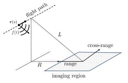
Figure 1. Setup for synthetic aperture radar imaging.

We use the start-stop approximation, which is typically done in SAR imaging. This approximation assumes that the change in displacement between the targets and the platform is negligibly small compared to the travel time it takes for the pulse emitted to propagate to the imaging scene and return as echoes. This approximation is valid in radar since the speed of light is orders of magnitude larger than the speed of the targets and the platform.

Using this start-stop approximation, we the consider the measurements only at $N$ discrete values of $s$, corresponding to $d(s_{n},t)$ for $n=1,\cdots,N$. Next, we suppose that $d(s_{n},t)$ is digitally sampled at $2M-1$ values of $t$. Consequently, these data have a discrete Fourier transform denoted by $d_{n}(\omega)$ evaluated at $2M-1$ frequencies denoted by $\omega_{m}$ for $m=1,\cdots,2M-1$. This choice of $2M-1$ samples is to make the notation in Section 3 simpler. With these assumptions, we find that our measurement data is given by the $2M-1\times N$ matrix $D$ whose columns are

(1) $$\mathbf{d}_{n}=\begin{bmatrix}d_{n}(\omega_{1})\\ d_{n}(\omega_{2})\\ \vdots\\ d_{n}(\omega_{2M-1})\end{bmatrix},\quad n=1,\cdots,N.$$

3. Rearranging frequency data

The data matrix $D$ is not suitable for direct application of signal subspace methods. Therefore, we introduce a rearrangement of the data based on the Prony method [18] which, for the $n$-th column of $D$, yields the following $M\times M$ matrix,

(2) $$D_{n}=\begin{bmatrix}d_{n}(\omega_{1})&d_{n}(\omega_{2})&\cdots&d_{n}(\omega_{M})\\ d_{n}(\omega_{2})&d_{n}(\omega_{3})&\cdots&d_{n}(\omega_{M+1})\\ \vdots&\vdots&\ddots&\vdots\\ d_{n}(\omega_{M})&d_{n}(\omega_{M+1})&\cdots&d_{n}(\omega_{2M-1})\end{bmatrix}.$$

In this rearrangement, the first column is the truncation of $\mathbf{d}_{n}$ to its first $M$ entries. Subsequent columns are sequential upward shifts of $\mathbf{d}_{n}$ truncated to its first $M$ entries.

To see why this rearrangement is suitable for signal subspace imaging, consider the Born approximation for a single point target. Let $\rho_{0}$ denote the reflectivity of the point target and $\boldsymbol{y}_{0}$ denote its position. According to the Born approximation, the scattered field at frequency $\omega_{m}$ is the spherical wave,

(3) $$\psi^{s}(\boldsymbol{x},\omega_{m})=\rho_{0}\frac{e^{\mathrm{i}\omega_{m}|\boldsymbol{x}-\boldsymbol{y}_{0}|/c}}{4\pi|\boldsymbol{x}-\boldsymbol{y}_{0}|}\psi^{inc}(\boldsymbol{y}_{0},\omega_{m}),$$

with $c$ denoting the wave speed and $\psi^{inc}(\boldsymbol{y}_{0},\omega_{m})$ denoting the field incident on the point target. Suppose that the signal emitted at position $\boldsymbol{x}_{n}$ on the flight path at frequency $\omega_{m}$ is a spherical wave with unit amplitude. For that case, the measurement $d_{n}(\omega_{m})$ corresponding to the scattered field evaluated at $\boldsymbol{x}_{n}$ is given by

(4) $$d_{n}(\omega_{m})=\rho_{0}\frac{e^{\mathrm{i}2\omega_{m}|\boldsymbol{x}_{n}-\boldsymbol{y}_{0}|/c}}{(4\pi|\boldsymbol{x}_{n}-\boldsymbol{y}_{0}|)^{2}}.$$

It follows that

(5) $$\mathbf{d}_{n}=\frac{\rho_{0}}{(4\pi|\boldsymbol{x}_{n}-\boldsymbol{y}_{0}|)^{2}}\begin{bmatrix}e^{\mathrm{i}2\omega_{1}|\boldsymbol{x}_{n}-\boldsymbol{y}_{0}|/c}\\ e^{\mathrm{i}2\omega_{2}|\boldsymbol{x}_{n}-\boldsymbol{y}_{0}|/c}\\ \vdots\\ e^{\mathrm{i}2\omega_{2M-1}|\boldsymbol{x}_{n}-\boldsymbol{y}_{0}|/c}\end{bmatrix},$$

from which we find that

(6) $$D_{n}=\frac{\rho_{0}}{(4\pi|\boldsymbol{x}_{n}-\boldsymbol{y}_{0}|)^{2}}\begin{bmatrix}e^{\mathrm{i}2\omega_{1}|\boldsymbol{x}_{n}-\boldsymbol{y}_{0}|/c}&e^{\mathrm{i}2\omega_{2}|\boldsymbol{x}_{n}-\boldsymbol{y}_{0}|/c}&\cdots&e^{\mathrm{i}2\omega_{M}|\boldsymbol{x}_{n}-\boldsymbol{y}_{0}|/c}\\ e^{\mathrm{i}2\omega_{2}|\boldsymbol{x}_{n}-\boldsymbol{y}_{0}|/c}&e^{\mathrm{i}2\omega_{3}|\boldsymbol{x}_{n}-\boldsymbol{y}_{0}|/c}&\cdots&e^{\mathrm{i}2\omega_{M+1}|\boldsymbol{x}_{n}-\boldsymbol{y}_{0}|/c}\\ \vdots&\vdots&\ddots&\vdots\\ e^{\mathrm{i}2\omega_{M}|\boldsymbol{x}_{n}-\boldsymbol{y}_{0}|/c}&e^{\mathrm{i}2\omega_{M+1}|\boldsymbol{x}_{n}-\boldsymbol{y}_{0}|/c}&\cdots&e^{\mathrm{i}2\omega_{2M-1}|\boldsymbol{x}_{n}-\boldsymbol{y}_{0}|/c}\end{bmatrix}.$$

Next, suppose that the frequencies are sampled according to $\omega_{m}=\omega_{1}+(m-1)\Delta\omega$ for $m=1,\cdots,2M-1$ with $\Delta\omega$ a fixed constant. For that case, we can rewrite (6) as $D_{n}=\sigma_{0}^{(n)}\mathbf{u}_{0}^{(n)}(\mathbf{v}_{0}^{(n)})^{\ast}$ with $\sigma_{0}^{(n)}=M|\rho_{0}|/(4\pi|\boldsymbol{x}_{n}-\boldsymbol{y}_{0}|)^{2}$,

(7) $$\mathbf{u}_{0}^{(n)}=\frac{e^{\mathrm{i}\theta_{0}/2}}{\sqrt{M}}\begin{bmatrix}e^{\mathrm{i}2\omega_{1}|\boldsymbol{x}_{n}-\boldsymbol{y}_{0}|/c}\\ e^{\mathrm{i}2\omega_{2}|\boldsymbol{x}_{n}-\boldsymbol{y}_{0}|/c}\\ \vdots\\ e^{\mathrm{i}2\omega_{M}|\boldsymbol{x}_{n}-\boldsymbol{y}_{0}|/c}\end{bmatrix},\quad\text{and}\quad\mathbf{v}_{0}^{(n)}=\frac{e^{-\mathrm{i}\theta_{0}/2}}{\sqrt{M}}\begin{bmatrix}1\\ e^{-\mathrm{i}2\Delta\omega|\boldsymbol{x}_{n}-\boldsymbol{y}_{0}|/c}\\ \vdots\\ e^{-\mathrm{i}2(M-1)\Delta\omega|\boldsymbol{x}_{n}-\boldsymbol{y}_{0}|/c}\end{bmatrix}.$$

Here, we have written the reflectivity as $\rho_{0}=|\rho_{0}|e^{\mathrm{i}\theta_{0}}$ and included $e^{\mathrm{i}\theta_{0}}$ in $\mathbf{u}_{0}^{(n)}$ and $\mathbf{v}_{0}^{(n)}$ arbitrarily in (7).

Suppose there are $P$ non-interacting point targets in the region with reflectivities $\rho_{p}$ at positions $\boldsymbol{y}_{p}$ for $p=1,\cdots,P$. It follows that

(8) $$D_{n}=\sum_{p=1}^{P}\sigma_{p}^{(n)}\mathbf{u}_{p}^{(n)}(\mathbf{v}_{p}^{(n)})^{\ast}.$$

Here, $\sigma_{p}^{(n)}=M|\rho_{p}|/(4\pi|\boldsymbol{x}_{n}-\boldsymbol{y}_{p}|)^{2}$, and $\mathbf{u}_{p}^{(n)}$ and $\mathbf{v}_{p}^{(n)}$ are defined just like $\mathbf{u}_{0}^{(n)}$ and $\mathbf{v}_{0}^{(n)}$ in (7), but evaluated on $|\boldsymbol{x}_{n}-\boldsymbol{y}_{p}|$ instead. This expression for $D_{n}$ is a sum of $P$ outer products, each of which corresponds to an individual point target. This outer product representation for $D_{n}$ indicates that signal subspace methods may be effectively used on these matrices for imaging.

4. Quantitative signal subspace method

To combine the matrices formed using the Prony method, we consider the $MN\times MN$ block diagonal matrix,

(9) $$D_{\text{Prony}}=\begin{bmatrix}D_{1}&&&\\ &D_{2}&&\\ &&\ddots&\\ &&&D_{N}\end{bmatrix}.$$

Using the outer-product structure identified in (8), we can extend a recently developed quantitative signal subspace imaging method [11] to this block-diagonal Prony matrix as follows.

Suppose we compute the singular value decomposition for each block: $D_{n}=U_{n}\Sigma_{n}V_{n}^{\ast}$ for $n=1,\cdots,N$. According to (8), for $P$ point targets, the rank of each block will be $P$. Assuming that the signal-to-noise ratio (SNR) is sufficiently high, the first $P$ singular values residing in the diagonal entries of $\Sigma_{n}$ will be significantly larger than the others. Those first $P$ singular values correspond to the signal subspace. The remaining singular values correspond to the noise subspace. Since we can separate the first $P$ singular values, we are able to compute the pseudo-inverse,

(10) $$\Sigma_{n}^{+}=\frac{1}{\sigma_{1}}\text{diag}\left(1,\frac{\sigma_{2}}{\sigma_{1}},\cdots,\frac{\sigma_{P}}{\sigma_{1}},\frac{1}{\epsilon},\cdots,\frac{1}{\epsilon}\right),$$

with $\epsilon>0$ denoting a user-defined parameter.

For search point $\boldsymbol{y}$ in the imaging region, we introduce the illumination block-vector

(11) $$\mathbf{a}(\boldsymbol{y})=\begin{bmatrix}\mathbf{a}_{1}(\boldsymbol{y})\\ \vdots\\ \mathbf{a}_{N}(\boldsymbol{y})\end{bmatrix},\qquad\mathbf{a}_{n}(\boldsymbol{y})=\frac{1}{4\pi|\boldsymbol{x}_{n}-\boldsymbol{y}|}\begin{bmatrix}e^{\mathrm{i}2\omega_{1}|\boldsymbol{x}_{n}-\boldsymbol{y}|/c}\\ \vdots\\ e^{\mathrm{i}2\omega_{M}|\boldsymbol{x}_{n}-\boldsymbol{y}|/c}\end{bmatrix}.$$

Using (10) and (11), we compute the following imaging functional

(12) $$F_{\epsilon}(\boldsymbol{y})=\frac{1}{N}\mathbf{a}^{\ast}(\boldsymbol{y})\begin{bmatrix}U_{1}\Sigma_{1}^{+}U_{1}^{\ast}&&\\ &\ddots&\\ &&U_{N}\Sigma_{N}^{+}U_{N}^{\ast}\end{bmatrix}\mathbf{a}(\boldsymbol{y})=\frac{1}{N}\sum_{n=1}^{N}\mathbf{a}_{n}^{\ast}(\boldsymbol{y})U_{n}\Sigma_{n}^{+}U_{n}^{\ast}\mathbf{a}_{n}(\boldsymbol{y}).$$

We also consider another imaging functional. For that imaging functional, we introduce the complimentary illumination block-vector,

(13) $$\mathbf{b}(\boldsymbol{y})=\begin{bmatrix}\mathbf{b}_{1}(\boldsymbol{y})\\ \vdots\\ \mathbf{b}_{N}(\boldsymbol{y})\end{bmatrix},\qquad\mathbf{b}_{n}(\boldsymbol{y})=\frac{1}{4\pi|\boldsymbol{x}_{n}-\boldsymbol{y}|}\begin{bmatrix}1\\ e^{-\mathrm{i}2\Delta\omega|\boldsymbol{x}_{n}-\boldsymbol{y}|/c}\\ \vdots\\ e^{-\mathrm{i}2(M-1)\Delta\omega|\boldsymbol{x}_{n}-\boldsymbol{y}|/c}\end{bmatrix},$$

and compute

(14) $$R_{\epsilon}(\boldsymbol{y})=\frac{1}{N}\mathbf{b}^{\ast}(\boldsymbol{y})\begin{bmatrix}V_{1}\Sigma_{1}^{+}U_{1}^{\ast}&&\\ &\ddots&\\ &&V_{N}\Sigma_{N}^{+}U_{N}^{\ast}\end{bmatrix}\mathbf{a}(\boldsymbol{y})=\frac{1}{N}\sum_{n=1}^{N}\mathbf{b}_{n}^{\ast}(\boldsymbol{y})V_{n}\Sigma_{n}^{+}U_{n}^{\ast}\mathbf{a}_{n}(\boldsymbol{y}).$$

We form images through evaluation of $1/F_{\epsilon}(\boldsymbol{y})$ and $1/R_{\epsilon}(\boldsymbol{y})$ over an imaging region. We show below that the image formed using $F_{\epsilon}$ is useful for determining the location and magnitude of reflectivities for point targets and the image formed using $R_{\epsilon}$ is useful for determining the complex reflectivities for point targets.

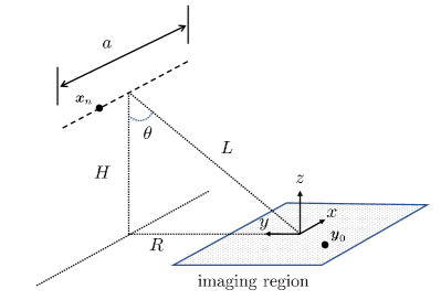
Figure 2. Sketch of the linear flight path over the planar imaging region used to study the resolution of the imaging method.

5. Resolution analysis

To study the performance of imaging using (12) and (14), we consider one point target located in a planar imaging region at position $\boldsymbol{y}_{0}$ with complex reflectivity $\rho_{0}$. We use a coordinate system in which the origin lies at the center of the planar imaging region. The flight path of the platform is linear and parallel to the $x$-axis. It is offset from the origin along the $y$-axis by range $R$ and along the $z$-axis by height $H$. Thus, spatial positions of the measurements are $\boldsymbol{x}_{n}=(x_{n},R,H)$ for $n=1,\cdots,N$ with $x_{n}=-a/2+a(n-1)/(N-1)$ and $a$ denoting the aperture. Let $L=\sqrt{R^{2}+H^{2}}$ denote the distance from the center of the flight path to the origin, and let $\theta$ denote the so-called look angle with $\sin\theta=R/L$ and $\cos\theta=H/L$. We assume that $L$ is the largest length scale in this problem. A sketch of this linear flight path over a planar imaging region is shown in Fig. 2.

To establish estimates for the resolution of image of one point target produced through evaluation of $1/F_{\epsilon}(\boldsymbol{y})$ over an imaging region, let $\boldsymbol{y}_{0}=(x_{0},y_{0},0)$ denote the target location, $\boldsymbol{y}=(x,y,0)$ denote the search location, and $B$ denote the system bandwidth centered at frequency $f_{0}$ with corresponding wavenumber $k_{0}=2\pi f_{0}/c$. With these quantities defined, we prove the following theorem.

Theorem 5.1 (Resolution estimates for a linear flight path).

Assuming that the SNR is sufficiently high that we can distinguish the singular values corresponding to the signal subspace from those corresponding to the noise subspace, $1/F_{\epsilon}(\boldsymbol{y})$ with $F_{\epsilon}(\boldsymbol{y})$ given in (12) attains a maximum of $|\rho_{0}|$ on $\boldsymbol{y}=\boldsymbol{y}_{0}$, and in the asymptotic limit, $L\gg 1$, $x_{0}/a\ll 1$, $y_{0}/R\ll 1$, and $\epsilon\ll 1$, this image has a cross-range resolution of $\Delta x^{\ast}=O(\sqrt{\epsilon}(c/B)(L/a))$ and a range resolution of $\Delta y^{\ast}=O(\sqrt{\epsilon}(c/B)(L/R))$.

Proof.

For a single point target, we have $D_{n}=\sigma_{0}^{(n)}\mathbf{u}_{0}^{(n)}\mathbf{v}_{0}^{(n)\ast}$ for $n=1,\cdots,N$ with $\sigma_{0}^{(n)}=M|\rho_{0}|/(4\pi|\boldsymbol{x}_{n}-\boldsymbol{y}_{0}|)^{2}$ and $\mathbf{u}_{0}^{(n)}$ and $\mathbf{v}_{0}^{(n)}$ given in (7). Consequently, the column space of $D_{n}$ is $\mathcal{C}(D_{n})=\text{span}\{\mathbf{u}_{0}^{(n)}\}$ and $P^{(n)}=I-\mathbf{u}_{0}^{(n)}\mathbf{u}_{0}^{(n)\ast}$ is the projection onto subspace orthogonal to $\mathcal{C}(D_{n})$. Using

$$\Sigma_{n}^{+}=\frac{1}{\sigma_{0}^{(n)}}\text{diag}\left(1,\frac{1}{\epsilon},\cdots,\frac{1}{\epsilon}\right),$$

we find that

$$F_{\epsilon}(\boldsymbol{y}) =\frac{1}{N}\sum_{n=1}^{N}\left[\frac{1}{\epsilon\sigma_{0}^{(n)}}\mathbf{a}_{n}^{\ast}(\boldsymbol{y})(I-\mathbf{u}_{0}^{(n)}\mathbf{u}_{0}^{(n)\ast})\mathbf{a}_{n}(\boldsymbol{y})+\frac{1}{\sigma_{0}^{(n)}}\mathbf{a}_{n}^{\ast}(\boldsymbol{y})\mathbf{u}_{0}^{(n)}\mathbf{u}_{0}^{(n)\ast}\mathbf{a}_{n}(\boldsymbol{y})\right]$$

(15) $$=\frac{1}{|\rho_{0}|}\frac{1}{N}\sum_{n=1}^{N}\left[\left(\frac{1}{\epsilon}-\left(\frac{1}{\epsilon}-1\right)|\Phi_{n}|^{2}\right)\frac{|\boldsymbol{x}_{n}-\boldsymbol{y}_{0}|^{2}}{|\boldsymbol{x}_{n}-\boldsymbol{y}|^{2}}\right],$$

where we have introduced the quantity,

(16) $$\Phi_{n}=\frac{1}{M}\sum_{m=1}^{M}e^{\mathrm{i}\omega_{m}\varDelta\tau_{n}},$$

with $\varDelta\tau_{n}=2(|\boldsymbol{x}_{n}-\boldsymbol{y}|-|\boldsymbol{x}_{n}-\boldsymbol{y}_{0}|)/c$ denoting the difference in travel times for the search and target locations.

Evaluating (15) on $\boldsymbol{y}_{0}$, we find that $F_{\epsilon}(\boldsymbol{y}_{0})=1/|\rho_{0}|$, so $1/F_{\epsilon}(\boldsymbol{y}_{0})=|\rho_{0}|$. Because $|\Phi_{n}|^{2}\leq 1$ and $|\boldsymbol{x}_{n}-\boldsymbol{y}_{0}|^{2}/|\boldsymbol{x}_{n}-\boldsymbol{y}|^{2}\leq 1$ with both functions evaluating to $1$ only at $\boldsymbol{y}=\boldsymbol{y}_{0}$, this result corresponds the maximum value that $1/F_{\epsilon}(\boldsymbol{y})$ attains.

Let

$$\omega_{m}=\omega_{0}\left[1+\beta\left(\frac{m-1}{M-1}-\frac{1}{2}\right)\right],\quad m=1,\cdots,M,$$

with $\beta=2\pi B/\omega_{0}$ denoting the fraction of the bandwith about the central frequency. Substituting these frequencies into (16) and computing the sum, we find

$$\Phi_{n}=\frac{e^{\mathrm{i}\omega_{0}(1-\beta/2)\varDelta\tau_{n}}}{M}\frac{1-e^{\mathrm{i}\omega_{0}\beta M\varDelta\tau_{n}/(M-1)}}{1-e^{\mathrm{i}\omega_{0}\beta\varDelta\tau_{n}/(M-1)}},$$

from which it follows that

$$|\Phi_{n}|^{2}=\frac{1}{M^{2}}\frac{\sin^{2}\left(\frac{\pi MB\varDelta\tau_{n}}{M-1}\right)}{\sin^{2}\left(\frac{\pi B\varDelta\tau_{n}}{M-1}\right)}.$$

In the expression above, we have resubstituted $\omega_{0}\beta=2\pi B$. Assuming we are in a small neighborhood about the target location, we expand the expression above about $\varDelta\tau_{n}=0$ and obtain

$$|\Phi_{n}|^{2}=1-\frac{\pi^{2}B^{2}}{3}\frac{M+1}{M-1}\varDelta\tau_{n}^{2}+O(\varDelta\tau_{n}^{4}).$$

Additionally, we find that

$$\frac{|\boldsymbol{x}_{n}-\boldsymbol{y}_{0}|}{|\boldsymbol{x}_{n}-\boldsymbol{y}|}=\frac{(x_{n}-x_{0})^{2}+(L\sin\theta-y_{0})^{2}+(L\cos\theta)^{2}}{(x_{n}-x)^{2}+(L\sin\theta-y)^{2}+(L\cos\theta)^{2}}=1+O(L^{-1}),$$

where $\sin\theta=R/L$ and $\cos\theta=H/L$. Using these approximations, we find that

(17) $$F_{\epsilon}(\boldsymbol{y})=\frac{1}{|\rho_{0}|}\left[1+\left(\frac{1}{\epsilon}-1\right)\frac{\pi^{2}B^{2}}{3}\frac{M+1}{M-1}\left(\frac{1}{N}\sum_{n=1}^{N}\varDelta\tau_{n}^{2}\right)\right]+O(\varDelta\tau_{n}^{4},L^{-1}).$$

Next, we use

(18) $$\varDelta\tau_{n}=(|\boldsymbol{x}_{n}-\boldsymbol{y}|-|\boldsymbol{x}_{n}-\boldsymbol{y}_{0}|)/c=\cos\theta\frac{(y-y_{0})}{c}\\ +\frac{(x-x_{0})^{2}-2(x-x_{0})(\xi_{n}-x_{0})}{2cL}+\sin^{2}\theta\frac{(y-y_{0})^{2}+2(y-y_{0})y_{0}}{2cL}+O(L^{-2}).$$

For the cross-range resolution, we evaluate (18) on $y=y_{0}$ and find that

$$\varDelta\tau_{n}^{2}\big{|}_{y=y_{0}}\sim\frac{(x-x_{0})^{2}}{c^{2}L^{2}}(x_{n}-x_{0})^{2}.$$

Using $x_{n}=-a/2+a(n-1)/(N+1)$, we find that

$$\frac{1}{N}\sum_{n=1}^{N}(x_{n}-x_{0})^{2}=\frac{a^{2}}{12}\frac{N+1}{N-1}+x_{0}^{2},$$

and so

$$F_{\epsilon}(x,y_{0})\sim\frac{1}{|\rho_{0}|}\left[1+\left(\frac{1}{\epsilon}-1\right)\frac{\pi^{2}B^{2}a^{2}}{3c^{2}L^{2}}\frac{M+1}{M-1}\left(\frac{1}{12}\frac{N+1}{N-1}+\frac{x_{0}^{2}}{a^{2}}\right)(x-x_{0})^{2}\right].$$

The full-width/half-maximum (FWHM) in cross-range $\Delta x^{\ast}$ satisfies $1/F_{\epsilon}(x_{0}+\Delta x^{\ast},y_{0})=1/(2|\rho_{0}|)$. Substituting the approximation above into this definition, solving for $\Delta x^{\ast}$, and expanding that result about $\epsilon=0$, we find

$$\Delta x^{\ast} =\pm\sqrt{\epsilon}\frac{c}{B}\frac{L}{a}\frac{6}{\pi}\sqrt{\frac{M-1}{M+1}}\sqrt{\frac{N-1}{(N+1)+12(N-1)(x_{0}^{2}/a^{2})}}+O(\epsilon^{3/2})$$

$$=\pm\sqrt{\epsilon}\frac{c}{B}\frac{L}{a}\frac{6}{\pi}\sqrt{\frac{M-1}{M+1}}\sqrt{\frac{N-1}{N+1}}+O\left(\epsilon^{3/2},\frac{x_{0}^{2}}{a^{2}}\right)$$

$$=O\left(\sqrt{\epsilon}\frac{c}{B}\frac{L}{a}\right).$$

For the range resolution, we evaluate (18) on $x=x_{0}$ and find that

$$\varDelta\tau_{n}^{2}\big{|}_{x=x_{0}}=\frac{(y-y_{0})^{2}}{c^{2}}\left(\cos\theta-\sin^{2}\theta\frac{y_{0}}{L}\right)^{2}.$$

It follows that

$$F_{\epsilon}(x_{0},y)\sim\frac{1}{|\rho_{0}|}\left[1+\left(\frac{1}{\epsilon}-1\right)\frac{\pi^{2}B^{2}}{3c^{2}}\frac{M+1}{M-1}\left(\cos\theta-\sin^{2}\theta\frac{y_{0}}{L}\right)^{2}(y-y_{0})^{2}\right].$$

The full-width/half-maximum (FWHM) in range $\Delta y^{\ast}$ satisfies $1/F_{\epsilon}(x_{0},y_{0}+\Delta y^{\ast})=1/(2|\rho_{0}|)$. Substituting the approximation above into this definition, resubstituting $\cos\theta=R/L$, solving for $\Delta y^{\ast}$, and expanding that result about $\epsilon=0$, we find

$$\Delta y^{\ast} =\pm\sqrt{\epsilon}\frac{c}{B}\frac{L}{R}\frac{1}{1-\sin^{2}\theta(y_{0}/R)}\frac{\sqrt{3}}{\pi}\sqrt{\frac{M-1}{M+1}}+O(\epsilon^{3/2})$$

$$=\pm\frac{\sqrt{3}}{\pi}\sqrt{\epsilon}\frac{c}{B}\frac{L}{R}+O\left(\epsilon^{3/2},\frac{y_{0}}{R}\right)$$

$$=O\left(\sqrt{\epsilon}\frac{c}{B}\frac{L}{R}\right).$$

This completes the proof. ∎

Theorem 5.1 states that images of a point target formed through evaluation of $1/F_{\epsilon}(\boldsymbol{y})$ with $F_{\epsilon}(\boldsymbol{y})$ given in (12) will form an image that is peaked at the location of the target with magnitude equal to $|\rho_{0}|$. Because the user-defined parameter $\epsilon$ can be made arbitrarily small, this imaging method will yield high-resolution images provided that there is sufficient signal that the non-trivial singular values provide accurate quantitative data.

In general, the reflectivity of a point target is complex. To recover the complex reflectivity, we make use of the following theorem.

Theorem 5.2 (Recovery of the complex reflectivity).

For a point target located at $\boldsymbol{y}_{0}$ with complex reflectivity $\rho_{0}$, when the SNR is sufficient high that we can distinguish the signal subspace from the noise subspace, $1/R_{\epsilon}(\boldsymbol{y}_{0})=\rho_{0}$ with $R_{\epsilon}(\boldsymbol{y})$ given in (14).

Proof.

Through direct evaluation of $R_{\epsilon}$ given in (14) on $\boldsymbol{y}=\boldsymbol{y}_{0}$, we find $R_{\epsilon}(\boldsymbol{y}_{0})=e^{-\mathrm{i}\theta_{0}}/|\rho_{0}|$. It follows that $1/R_{\epsilon}(\boldsymbol{y}_{0})=|\rho_{0}|e^{\mathrm{i}\theta_{0}}=\rho_{0}$. ∎

Although Theorem 5.2 states that evaluating $1/R_{\epsilon}(\boldsymbol{y})$ yields the complex reflectivity, it is not generally useful for determining the location of the target because this function does not exhibit localized behavior that indicates the region about the target location. For this reason, we propose the following two-stage imaging method.

1. Evaluate $1/F_{\epsilon}(\boldsymbol{y})$ with $F_{\epsilon}(\boldsymbol{y})$ given in (12) to determine the location of targets. The value of $\epsilon$ may be varied to adjust the resolution of this image.

2. Evaluate $1/R_{\epsilon}(\boldsymbol{y})$ with $R_{\epsilon}(\boldsymbol{y})$ given in (14) using the locations determined in (i) to determine the complex reflectivities of the targets.

6. Travel time uncertainty

We now consider the effect of uncertainty in the travel times on images formed through evaluation of $1/F_{\epsilon}(\boldsymbol{y})$ with $F_{\epsilon}(\boldsymbol{y})$ given in (12). Uncertainty in travel times can arise from sampling clock jitter, deviations from the assumed flight path, and random fluctuations in the propagating medium among other practical issues. It is therefore important to understand to what extent images formed using the method described above are useful under uncertain conditions.

To model travel time uncertainty, we use

(19) $$\varDelta\tau_{n}=\varDelta\tau_{n}^{0}+\nu_{n},\quad n=1,\cdots,N.$$

with $\varDelta\tau_{n}^{0}$ denoting the difference in travel times for a homogeneous medium and the vector, $\boldsymbol{\nu}=(\nu_{1},\cdots,\nu_{N})$ denoting a multivariate distribution with $\mathbb{E}[\nu_{n}]=0$ and $\mathbb{E}[\nu_{n}^{2}]=\sigma_{n}^{2}$ for $n=1,\cdots,N$. Let $\sigma^{2}=\max\{\sigma_{1}^{2},\cdots\sigma_{N}^{2}\}$. Using this model for travel time uncertainty, we prove the following theorem.

Theorem 6.1 (Travel time uncertainty).

Assuming that the SNR is sufficiently high that we can distinguish the singular values corresponding to the signal subspace from those corresponding to the noise subspace, the image formed through evaluation of $1/F_{\epsilon}(\boldsymbol{y})$ in a neighborhood about $\boldsymbol{y}=\boldsymbol{y}_{0}$ with $F_{\epsilon}(\boldsymbol{y})$ given in (12) and using (19) with $\sigma^{2}/\epsilon\ll 1$ has an expected value whose leading behavior is the result for the homogeneous medium plus a term that is $O(\sigma^{2}/\epsilon)$, and has a variance that is $O(\sigma^{2}/\epsilon)$.

Proof.

Since we consider a neighborhood about $\boldsymbol{y}=\boldsymbol{y}_{0}$, we start with (17) and write

$$F_{\epsilon}\sim\frac{1}{|\rho_{0}|}\left[1+\alpha\left(\frac{1}{\epsilon}-1\right)\left(\frac{1}{N}\sum_{n=1}^{N}\varDelta\tau_{n}^{2}\right)\right],$$

with $\alpha=\pi^{2}B^{2}(M+1)/(3(M-1))$. Substituting (19) yields

$$F_{\epsilon}\sim\frac{1}{|\rho_{0}|}\left[1+\alpha\left(\frac{1}{\epsilon}-1\right)\left(\frac{1}{N}\sum_{n=1}^{N}\left(\varDelta\tau_{n}^{0}+\nu_{n}\right)^{2}\right)\right].$$

Based on our resolution estimates, we introduce the stretched variables $\varDelta\tau_{n}=\sqrt{\epsilon}\varDelta T_{n}$ for $n=1,\cdots,N$, and obtain

$$F_{\epsilon}\sim\frac{1}{|\rho_{0}|}\left[1+\alpha\left(1-\epsilon\right)\left(\frac{1}{N}\sum_{n=1}^{N}\left(\varDelta T_{n}+\nu_{n}/\sqrt{\epsilon}\right)^{2}\right)\right].$$

Let $f_{Y}(y_{1},\cdots,y_{N})$ denote the probability density function for $(\nu_{1},\cdots,\nu_{N})$. The expected value of the image is then

$$\mathbb{E}\left[\frac{1}{F_{\epsilon}}\right]\sim|\rho_{0}|\int\cdots\int\frac{f_{Y}(y_{1},\cdots,y_{N})}{1+\alpha\left(1-\epsilon\right)\left(\displaystyle\frac{1}{N}\sum_{n=1}^{N}\left(\varDelta T_{n}+y_{n}/\sqrt{\epsilon}\right)^{2}\right)}\mathrm{d}y_{1}\cdots\mathrm{d}y_{N}.$$

Substituting $y_{n}=\sigma\eta_{n}$ yields

$$\mathbb{E}\left[\frac{1}{F_{\epsilon}}\right]\sim|\rho_{0}|\int\cdots\int\frac{\sigma^{N}f_{Y}(\sigma\eta_{1},\cdots,\sigma\eta_{N})}{1+\alpha\left(1-\epsilon\right)\left(\displaystyle\frac{1}{N}\sum_{n=1}^{N}\left(\varDelta T_{n}+\sigma\eta_{n}/\sqrt{\epsilon}\right)^{2}\right)}\mathrm{d}\eta_{1}\cdots\mathrm{d}\eta_{N}.$$

Assuming that $\delta=\sigma/\sqrt{\epsilon}\ll 1$, we expand about $\delta=0$ and find

$$\left[1+\alpha\left(1-\epsilon\right)\left(\displaystyle\frac{1}{N}\sum_{n=1}^{N}\left(\varDelta T_{n}+\delta\eta_{n}\right)^{2}\right)\right]^{-1}=I_{0}-2\delta\alpha(1-\epsilon)I_{0}^{2}\left(\frac{1}{N}\sum_{n=1}^{N}\varDelta T_{n}\eta_{n}\right)+O(\delta^{2}),$$

with

$$I_{0}=\left[1+\alpha(1-\epsilon)\frac{1}{N}\sum_{n=1}^{N}(\varDelta T_{n})^{2}\right]^{-1},$$

denoting the normalized image formed in the homogeneous medium. Substituting this expansion into the integral above for the expected value of the image and using $\mathbb{E}[\nu_{n}]=0$ for $n=1,\cdots,N$, we find that

$$\mathbb{E}\left[\frac{1}{F_{\epsilon}}\right]=|\rho_{0}|I_{0}+O(\delta^{2}).$$

Next, by using the expansion

$$\left[1+\alpha\left(1-\epsilon\right)\left(\displaystyle\frac{1}{N}\sum_{n=1}^{N}\left(\varDelta T_{n}+\delta\eta_{n}\right)^{2}\right)\right]^{-2}=I_{0}^{2}-\delta\alpha(1-\epsilon)I_{0}^{3}\left(\sum_{n=1}^{N}\varDelta T_{n}\eta_{n}\right)+O(\delta^{2}),$$

we determine that

$$\mathbb{E}\left[\left(\frac{1}{F_{\epsilon}}\right)^{2}\right]=|\rho_{0}|^{2}I_{0}^{2}+O(\delta^{2}).$$

Therefore,

$$\text{Var}\left[\frac{1}{F_{\epsilon}}\right]=\mathbb{E}\left[\left(\frac{1}{F_{\epsilon}}\right)^{2}\right]-\left(\mathbb{E}\left[\frac{1}{F_{\epsilon}}\right]\right)^{2}=O(\delta^{2}).$$

∎

Theorem 6.1 states that when $\sigma/\sqrt{\epsilon}\ll 1$, the leading behavior of the expectation of the image with random perturbations to the travel time is exactly the same as the image in the homogeneous medium. The recovery of the magnitude of the reflectivity $|\rho_{0}|$, and the resolution estimates of Theorem 5.1 are different by a term that is $O(\sigma^{2}/\epsilon)$. Because the variance of the image is $O(\sigma^{2}/\epsilon)$, we determine that this image formed is statistically stable.

An immediate consequence of Theorem 6.1 is given in the following corollary.

Corollary 6.1.1 (Resolution with travel time uncertainty).

When $\sigma^{2}$ is known or can be reliably estimated, one can set the value of $\epsilon$ so that $\sigma^{2}\ll\epsilon$ and Theorem 6.1 will hold.

Setting $\epsilon$ in this way connects the resolution of the image with the variance of the random perturbations to the travel time.

7. Numerical results

To validate the theoretical results from above, we use numerical simulations to generate data for various scattering scenes. The following values for the parameters are based on the GOTCHA data set [5]. In particular, we have set $R=3.55\,\text{km}$ and $H=7.30\,\text{km}$, so that $L=\sqrt{H^{2}+R^{2}}=8.12\,\text{km}$. The synthetic aperture created by the linear flight path is $a=0.13\,\text{km}$. The central frequency is $f_{0}=9.6\,\text{GHz}$ and the bandwidth is $B=622\,\text{MHz}$. Using $c=3\times 10^{8}\,\text{m/s}$, we find that the central wavelength is $\lambda_{0}=3.12\,\text{cm}$. The imaging region is at the ground level $z=0$. We use $2M-1=39$ frequencies so that $M=20$, and $N=32$ spatial measurements.

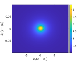
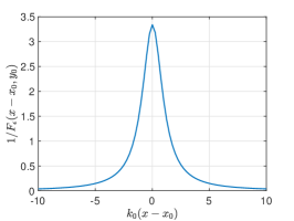
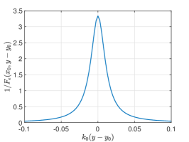
Figure 3. Image formed through evaluation of $1/F_{\epsilon}(\boldsymbol{y})$ with $F_{\epsilon}(\boldsymbol{y})$ given in (12) for a point target located at $x_{0}=y_{0}=1\,\text{m}$ on the planar imaging region. Measurement noise was added so that $\text{SNR}=44.1339\text{dB}$. For this image, $\epsilon=10^{-8}$.

7.1. Single point target

We first consider imaging a single point target located at $x_{0}=y_{0}=1\,\text{m}$ with complex reflectivity $\rho_{0}=3.4\mathrm{i}$ on the planar imaging region. Figure 3 shows the image formed through evaluation of $1/F_{\epsilon}(\boldsymbol{y})$ with $F_{\epsilon}(\boldsymbol{y})$ given in (12) with $\epsilon=10^{-10}$. Measurement noise was added so that the signal-to-noise ratio (SNR) is $\text{SNR}=44.1339\,\text{dB}$. The left plot of Fig. 3 shows the color contour plot of the image in a region about the target location. The center plot of Fig. 3 shows the image on $y=y_{0}$ as a function of $x$ (cross-range), and the right plot shows the image on $x=x_{0}$ as a function of $y$ (range). These results shown in Fig. 3 show that the image attains its maximum value of $3.4$ corresponding to $|\rho_{0}|$ at the correct target location. The image attains a high resolution due to choice of $\epsilon$. Because $L/R=2.29$ and $L/a=62.46$, we expect from the resolution estimates given in Theorem 5.1 that the range resolution should be better than the cross-range resolution. This difference in resolution can be observed by noting the values of $k_{0}(x-x_{0})$ in the center plot compared to the values of $k_{0}(y-y_{0})$ in the right plot of Fig. 3.

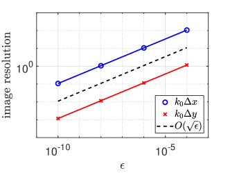
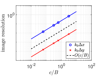
Figure 4. Numerically computed image resolutions with respect to $\epsilon$ (left) and $c/B$ (right). The range resolutions, $k_{0}\Delta x$, are plotted as “$\circ$” symbols, and the cross-range resolution, $k_{0}\Delta y$, are plotted as red “$\times$” symbols. The blue and red curves are the least-squares fit to lines through the range and cross-range resolution data, respectively.

In Fig. 4 we show numerically computed FWHM values of $k_{0}\Delta x$ (cross-range resolution) and $k_{0}\Delta y$ (range resolution) for a single point target when varying $\epsilon$ (left plot) and $c/B$ (right plot). The blue “$\circ$” symbols are the computed values of $k_{0}\Delta x$ and the red “$\times$” symbols are the computed values of $k_{0}\Delta y$ both found by numerically determining the FWHM. The solid blue and red curves are the least-squares linear fit through the $\Delta x$ and $\Delta y$ data, respectively. For the results shown in the left plot of Fig. 4, all parameters are set to the same values used for Fig. 3, except that $\text{SNR}=\infty$, so there is no noise. For the right plot of Fig. 4, we have varied the value of $B$, but all other parameter values are the same as those used for Fig. 3. In these results, we find that $k_{0}\Delta x>k_{0}\Delta y$ for all values of $\epsilon$ and $c/B$ which is due to the fact that $L/R<L/a$.

The results for cross-range and range resolutions with respect to $\epsilon$ given in the left plot of Fig. 4 clearly show an $O(\sqrt{\epsilon})$ behavior which is plotted as a dashed-black curve in the left plot of Fig. 4. The computed least-squares fits are $\log(\Delta x)\approx 3.9593+0.4991\log(\epsilon)$ and $\log(\Delta y)\approx-0.5565+0.4992\log(\epsilon)$ which numerically validate this $O(\sqrt{\epsilon})$ behavior.

The results for cross-range and range resolutions with respect to $c/B$ given in the right plot of Fig. 4 clearly show an $O(c/B)$ behavior which is plotted as a dashed-black curve. The least-squares fits are $\log(\Delta x)\approx-6.8067+0.9997\log(c/B)$ and $\log(\Delta y)\approx-11.3247+0.9999\log(c/B)$ which numerically validate the $O(c/B)$ behavior.

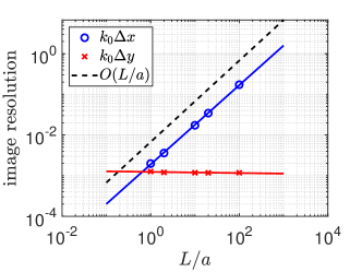
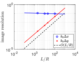
Figure 5. Numerical computed image resolutions with respect to $L/a$ (left) and $L/R$ (right). The cross-range resolutions, $k_{0}\Delta x$, are plotted as “$\circ$” symbols, and the range resolutions, $k_{0}\Delta y$, are plotted as red “$\times$” symbols. The blue and red curves are the least-squares fit to lines through the cross-range and range resolution data, respectively.

The behaviors of computed image resolution with respect to $L/a$ and $L/R$ are shown in Fig. 5. For these results, all parameter values are the same as those used for Fig. 3 except that $\text{SNR}=\infty$, so there is no noise and $a$ is varied in the left plot and $R$ is varied in the right plot. The computed range and cross-range FWHM values, $k_{0}\Delta x$ and $k_{0}\Delta y$, respectively, are plotted just as in Fig. 4 including the corresponding least-squares fit to lines.

The results for cross-range resolution with respect to $L/a$ shown in the left plot of Fig. 5 clearly show an $O(L/a)$ behavior, which is plotted as a dashed-black curve. The computed least-squares fit to a line is $\log(\Delta x)\approx-11.5748+0.9741\log(L/a)$ which numerically validates the $O(L/a)$ behavior. In contrast, the range resolution does not vary significantly with $L/a$. The computed least-squares fit to a line is $\log(\Delta y)\approx-12.0007-0.0139\log(L/a)$ which quantifies the weak dependence that range resolution has on aperture.

The results for range resolution with respect to $L/R$ shown in the right plot of Fig. 5 clearly show an $O(L/R)$ behavior, which is plotted as a dashed-black curve. The computed least-squares fit to a line is $\log(\Delta y)\approx-12.8645+0.9690\log(L/R)$ which numerically validates this $O(L/R)$ behavior. In contrast, the cross-range resolution shows a much weaker dependence on $L/R$. The computed least-squares fit to a line is $\log(\Delta x)\approx-7.5134-0.0340\log(L/R)$ which quantifies this weak dependence on $L/R$.

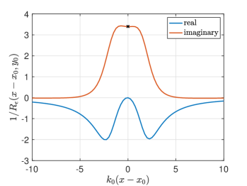
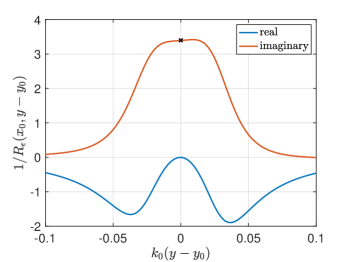
Figure 6. Recovering the complex reflectivity through evaluation of $1/R_{\epsilon}(\boldsymbol{y})$ with $R_{\epsilon}(\boldsymbol{y})$ given in (14) with $\epsilon=10^{-10}$. Measurement noise was added so that $\text{SNR}=44.1339\text{dB}$. The left plot shows $1/R_{\epsilon}$ on $y=y_{0}$ as a function of $x-x_{0}$ and the right plot shows $1/R_{\epsilon}$ on $x=x_{0}$ as a function of $y-y_{0}$. The blue curves give the real part of $1/R_{\epsilon}(\boldsymbol{y})$ and the red curves give the imaginary part. The black “$\times$” symbol gives the exact value of the complex reflectivity, $\rho_{0}=3.4\mathrm{i}$.

We now show results from evaluating $1/R_{\epsilon}(\boldsymbol{y})$ with $R_{\epsilon}(\boldsymbol{y})$ given in (14). These results use the same parameter values as those used in Fig. 3. When plotting $1/R_{\epsilon}$, there is no local behavior to indicate the location of the target. For this reason these images do not provide useful information about the location of targets. However, when we evaluate $1/R_{\epsilon}(\boldsymbol{y})$ in a region near the target location, we are able to recover the complex reflectivity. In Fig. 6 we show the real and imaginary parts of $1/R_{\epsilon}(x-x_{0},y_{0})$ in the left plot and of $1/R_{\epsilon}(x_{0},y-y_{0})$ in the right plot. In both plots the actual value $\rho_{0}=3.4\mathrm{i}$ is plotted as a black “$\times$” symbol. These plots show that when the location of the point target is known, evaluating $1/R_{\epsilon}(\boldsymbol{y})$ at the recovered target location provides a method for recovering the complex reflectivity. At the target location, we find $1/R_{\epsilon}(\boldsymbol{y}_{0})=-1.3059\times 10^{-3}+3.3928\mathrm{i}$ which demonstrates a very high accuracy in recovering the complex reflectivity. Provided that the target location is reasonably accurate, the user-defined parameter $\epsilon$ can be used to regularize these results to enable stable recovery of the complex reflectivity.

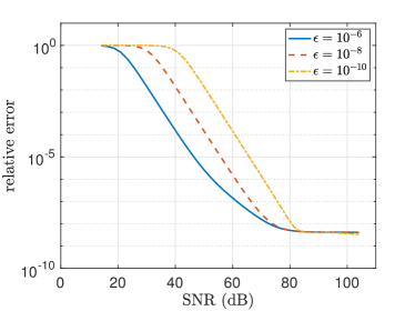
Figure 7. Relative error in the recovery of the complex reflectivity through evaluation of $1/R_{\epsilon}(\boldsymbol{y}_{0})$ with $\epsilon=10^{-8}$ for a point target as a function of SNR (dB). All parameters are the same as those used in Fig. 3.

In both Theorems 5.1 and 5.2, it is assumed that the SNR is sufficiently high that one can separate the signal subspace from the noise subspace. To investigate the effect of SNR on the recovery of the complex reflectivity, we evaluate $1/R_{\epsilon}(\boldsymbol{y}_{0})$ for different SNR values and compute the relative error, $E_{\text{rel}}=|\rho_{0}-1/R_{\epsilon}(\boldsymbol{y}_{0})|/|\rho_{0}|$. These relative error results are shown with $\epsilon=10^{-6}$ as a solid blue curve, $\epsilon=10^{-8}$ as a dashed red curve, and $\epsilon=10^{-10}$ as a dot-dashed yellow curve in Fig. 7. The results in Fig. 7 show that sufficiently high SNR is needed to achieve a high accuracy. Additionally, we observe that larger $\epsilon$ values achieve higher accuracy for any fixed SNR. This higher accuracy occurs because $\epsilon$ regularizes $1/R_{\epsilon}(\boldsymbol{y})$ thereby stabilizing the recovery of the complex reflectivity. The role of SNR on the resolution becomes more of an issue when imaging multiple targets which we discuss below.

7.2. Multiple point targets

We now consider multiple point targets in the imaging region. We set the origin of the coordinate system to lie at the center of a $5\,\text{m}\times 5\,\text{m}$ planar imaging region on $z=0$. The first target is located at $(x_{1},y_{1},0)=(0.01\,\text{m},0.1\,\text{m},0)$ with complex reflectivity $\rho_{1}=3.4\mathrm{i}$. The second target is located at $(x_{2},y_{2},0)=(-0.30\,\text{m},-0.50\,\text{m},0)$ with complex reflectivity $\rho_{2}=4.2\mathrm{i}$. The third target is located at $(x_{3},y_{3},0)=(-0.50\,\text{m},0.50\,\text{m},0)$ with complex reflectivity $\rho_{3}=3.1\mathrm{i}$.

(a) $\epsilon=10^{-6}$

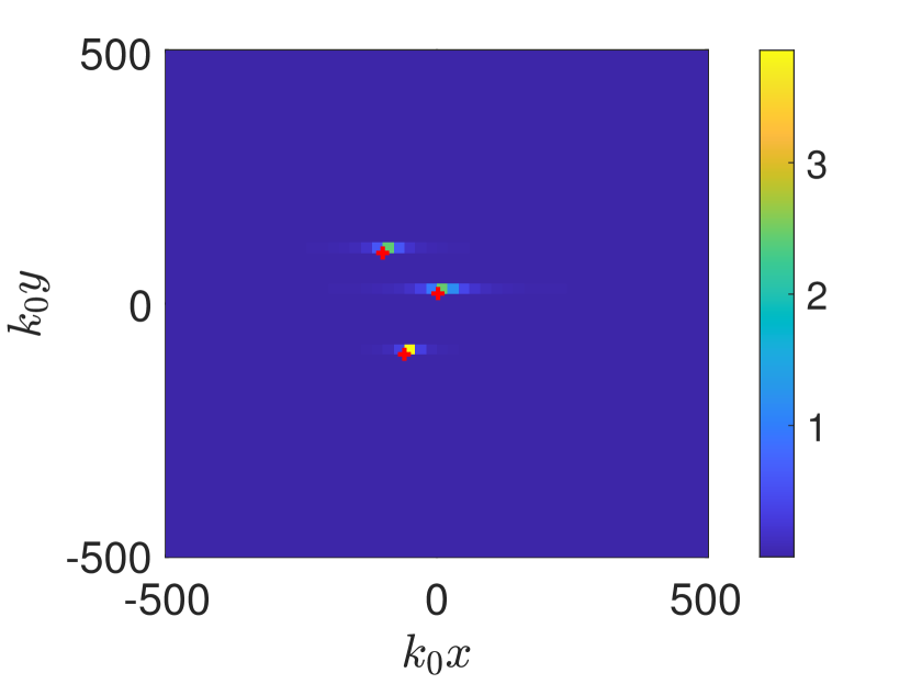
(b) $\epsilon=10^{-8}$

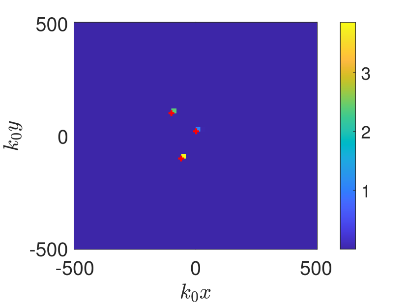
(c) $\epsilon=10^{-10}$

Figure 8. Imaging through evaluation of $1/F_{\epsilon}(\boldsymbol{y})$ with $F_{\epsilon}(\boldsymbol{y})$ given in (12) and $\epsilon=10^{-6}$ (left), $\epsilon=10^{-8}$ (center), and $\epsilon=10^{-10}$ (right) for 3 point targets with $\text{SNR}=64.1695\,\text{dB}$. The first target is located at $(x_{1},y_{1},0)=(0.01\,\text{m},0.1\,\text{m},0)$ with complex reflectivity $\rho_{1}=3.4\mathrm{i}$. The second target is located at $(x_{2},y_{2},0)=(-0.3\,\text{m},-0.5\,\text{m},0)$ with complex reflectivity $\rho_{2}=4.2\mathrm{i}$. The third target is located at $(x_{3},y_{3},0)=(-0.5\,\text{m},0.5\,\text{m},0)$ with complex reflectivity $\rho_{3}=3.1\mathrm{i}$.

In Fig. 8 we show the image produced through evaluation of $1/F_{\epsilon}(\boldsymbol{y})$ with $F_{\epsilon}(\boldsymbol{y})$ given in (12) with $\epsilon=10^{-6}$ (left), $\epsilon=10^{-8}$ (center), and $\epsilon=10^{-10}$ (right). The imaging region is discretized using a $51\times 51$ equi-spaced mesh corresponding to approximately a $10\,\text{cm}$ meshwidth. Measurement noise was added so that $\text{SNR}=64.1695\,\text{dB}$. We see that the value of $\epsilon$ affects the overall resolution of the three targets, especially with respect to cross-range since $L/a<L/R$. With $\epsilon=10^{-10}$, the image produced through evaluation of $1/F_{\epsilon}(\boldsymbol{y})$ clearly indicates the locations of the three targets. Even though we do not have direct interpretation of the magnitude of the peaks in this plot, we do find that $\|1/F_{\epsilon}(\boldsymbol{y})\|_{\infty}=3.8641$ for $\epsilon=10^{-10}$, which is close to the values of $|\rho_{1}|$, $|\rho_{2}|$, and $|\rho_{3}|$.

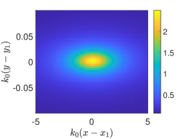
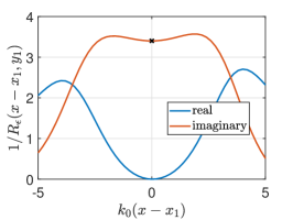
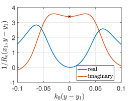
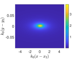
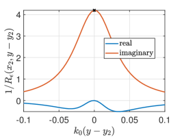
Figure 9. (left) Imaging using $1/F_{\epsilon}(\boldsymbol{y})$ in a region about target 1 located at $(x_{1},y_{1},0)=(0.01\,\text{m},0.1\,\text{m},0)$ with complex reflectivity $\rho_{1}=3.4\mathrm{i}$. Recovering the complex reflectivity through evaluation of $1/R_{\epsilon}(x-x_{1},y_{1})$ (center) and $1/R_{\epsilon}(x_{1},y-y_{1})$ (right). The blue curves give the real part of $1/R_{\epsilon}(\boldsymbol{y})$ and the red curves give the imaginary part. The black “$\times$” symbol gives the exact value of the complex reflectivity, $\rho_{1}=3.4\mathrm{i}$.

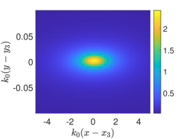
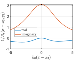
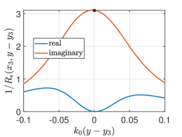
Figure 10. The same as Fig. 11, except for target 2 located at $(x_{2},y_{2},0)=(-0.30\,\text{m},-0.50\,\text{m},0)$ with complex reflectivity $\rho_{2}=4.2\mathrm{i}$.

Figure 11. The same as Fig. 11, except for target 3 located at $(x_{3},y_{3},0)(-0.50\,\text{m},0.50\,\text{m},0)$ with complex reflectivity $\rho_{3}=3.1\mathrm{i}$.

Using Fig. 8 to determine regions about each of the target locations, we then evaluate $1/F_{\epsilon}(\boldsymbol{y})$ using the same measurements to obtain the location more precisely and $1/R_{\epsilon}(\boldsymbol{y})$ to recover the complex reflectivities. In particular, we plotted the evaluation of $1/F_{\epsilon}(\boldsymbol{y})$ in a window of size $10\,k_{0}$ in cross-range ($x$) and $0.2\,k_{0}$ in range ($y$) about each target using a $51\times 51$ mesh. The results of doing this are shown in Fig. 11 for target 1, Fig. 11 for target 2, and Fig. 11 for target 3. The left plots in Figs. 11 – 11 show results of evaluating $1/F_{\epsilon}(\boldsymbol{y})$ in regions about the respective targets. The center plots in Figs. 11 – 11 shows results of evaluating $1/R_{\epsilon}(\boldsymbol{y})$ on $y=y_{1}$, $y_{2}$, and $y_{3}$, respectively, and the left plots in Figs. 11 – 11 shows results of evaluating $1/R_{\epsilon}(\boldsymbol{y})$ on $x=x_{1}$, $x_{2}$, and $x_{3}$, respectively.

When plotting $1/F_{\epsilon}(\boldsymbol{y})$ in a small region about each target location, we are readily able to determine the target location corresponding to where this function attains its local maximum thereby demonstrating the high-resolution of this imaging method. With the location of each target determined using these results, we then evaluate $1/R_{\epsilon}(\boldsymbol{y})$ in these regions which allows for recovery of the complex reflectivity of each target. For these results, these evaluations yielded $\rho_{1}=3.4\mathrm{i}\approx 4.0096\times 10^{-4}+3.3990\mathrm{i}$, $\rho_{2}=4.2\mathrm{i}\approx 1.4427\times 10^{-4}+4.2000\mathrm{i}$, and $\rho_{3}=3.1\mathrm{i}\approx 1.3969\times 10^{-4}+3.0998\mathrm{i}$ thereby demonstrating the high quantitative accuracy achieved using this method.

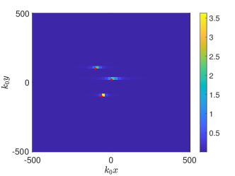
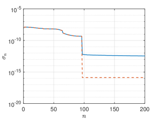
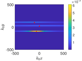
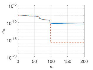
Figure 12. Image produced through evaluation of $1/F_{\epsilon}(\boldsymbol{y})$ with $F_{\epsilon}(\boldsymbol{y})$ given in (12) and $\epsilon=10^{-8}$ for $\text{SNR}=44.1695\,\text{dB}$ (top left), and the corresponding singular value spectrum (top right). The lower left and right plots are for $\text{SNR}=24.1695\,\text{dB}$. All parameter values are the same as those used in Fig. 8.

We showed the effect of SNR on the recovery of the complex reflectivity for a single point target in Fig. 7. To study the effect of SNR of imaging multiple point targets, we consider images for the same scenario produced through evaluation of $1/F_{\epsilon}(\boldsymbol{y})$ with $F_{\epsilon}(\boldsymbol{y})$ given in (12) and $\epsilon=10^{-8}$ for $\text{SNR}=44.1695\,\text{dB}$ (top row of Fig. 12) and $24.1695\,\text{dB}$ (bottom row of Fig. 12). Except for the SNR values, all parameter values are the same as those in Fig. 8(b). Included with each of those images are the corresponding singular value spectra for $D_{\text{Prony}}$ given in (9) plotted as blue curves. The dashed red curves show the thresholded singular values in which $\sigma_{n}$ is replaced with $\epsilon\sigma_{1}$ for all $\sigma_{n}<0.01\sigma_{1}$.

In Fig. 12, the image for $\text{SNR}=44.1695\,\text{dB}$ (top left) shows the three targets clearly, but the image for $\text{SNR}=24.1695\,\text{dB}$ (bottom left) has much poorer resolution, especially in range. The singular value spectra in Fig. 12 (top right and bottom left) provide valuable insight into the difference between these two images. A signal subspace method is predicated on the assumption that one can distinguish the signal and noise subspaces from one another. With regards to the singular value spectrum, one would like to have a large “gap” between the singular values corresponding to the signal subspace and those corresponding to the noise subspace. We observe in Fig. 12 that when the SNR decreases, so does the gap separating the singular values for the signal subspace from those of the noise subspace. Even though the thresholding criterion of replacing $\sigma_{n}$ with $\epsilon\sigma_{1}$ when $\sigma_{n}<0.01\sigma_{1}$ captures the location of the gap correctly for both SNR values, a consequence of the narrowing of this gap is a loss of image resolution. Because $L/a<L/R$, we see a more severe loss in resolution in range than in cross-range. These results demonstrate that this imaging method requires a sufficiently high SNR to be effective and accurate.

7.3. Imaging in random media

We consider perturbations in travel times resulting from wave propagation in random media. Assuming an inhomogeneous velocity profile of the form

(20) $$\frac{1}{c^{2}(\boldsymbol{x})}=\frac{1}{c_{0}^{2}}\left(1+\sigma\mu\left(\frac{\boldsymbol{x}}{\ell}\right)\right),$$

we approximate the Green’s function between points $\boldsymbol{x}$ and $\boldsymbol{y}$ at frequency $\omega$ by

(21) $$G(\boldsymbol{x},\boldsymbol{y};\omega)=G_{0}(\boldsymbol{x},\boldsymbol{y};\omega)\exp{\left[i\omega\nu(\boldsymbol{x},\boldsymbol{y})\right]},$$

with $\nu(\boldsymbol{x},\boldsymbol{y})$ denoting the random travel time function

(22) $$\nu(\boldsymbol{x},\boldsymbol{y})=\frac{\sigma|\boldsymbol{x}-\boldsymbol{y}|}{2c_{0}}\int_{0}^{1}\mu\left(\frac{\boldsymbol{y}}{\ell}+(\boldsymbol{x}-\boldsymbol{y})\frac{s}{\ell}\right)\mathrm{d}s.$$

Here $c_{0}$ denotes the average propagation speed, assumed constant, $\ell$ is the correlation length and $\sigma$ is the strength of the fluctuations. The stationary random process $\mu(\cdot)$ has mean zero and normalized auto-correlation function $R(|\boldsymbol{x}-\boldsymbol{x}^{\prime}|)=\mathbb{E}(\mu(\boldsymbol{x})\mu(\boldsymbol{x}^{\prime}))$, so that $R(0)=1$, and $\int_{0}^{\infty}R(r)r^{2}dr<\infty$. In (21), $G_{0}$ denotes the Green’s function in the homogeneous medium with propagation speed $c_{0}$.

(a) $\tilde{\sigma}/\sqrt{\epsilon}=0$

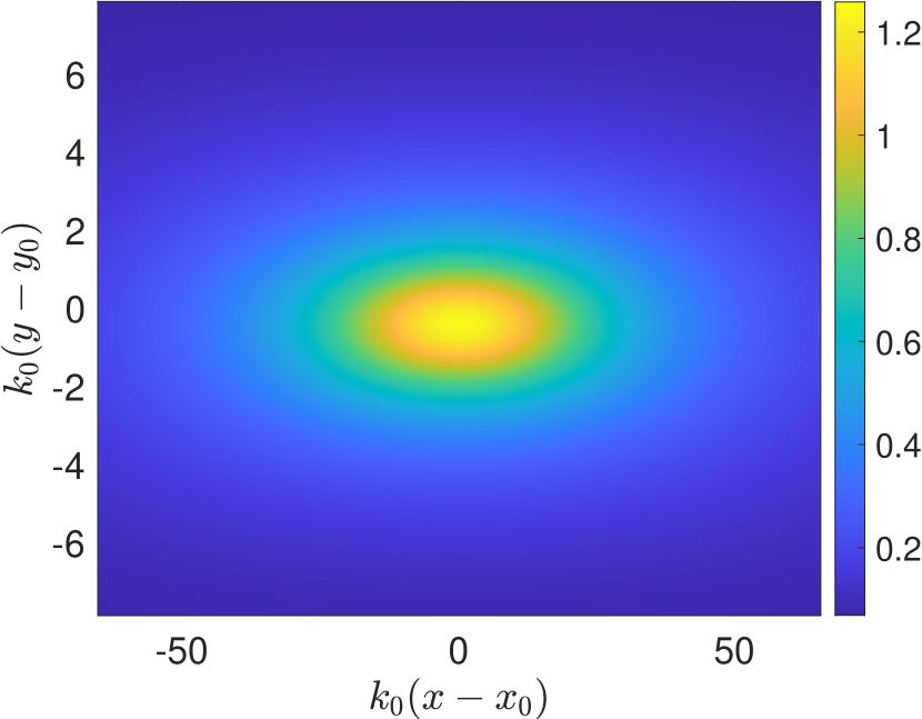
(b) $\tilde{\sigma}/\sqrt{\epsilon}=\epsilon$

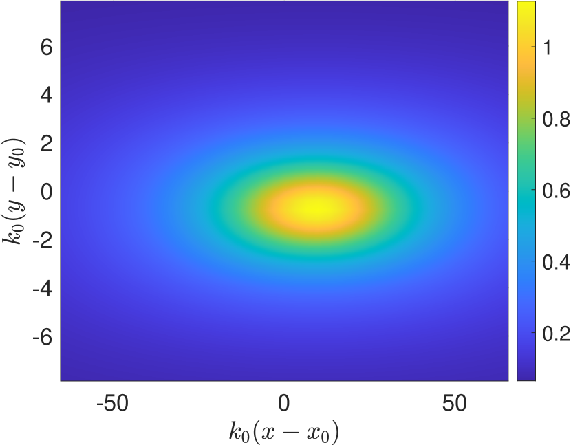
(c) $\tilde{\sigma}/\sqrt{\epsilon}=1$

Figure 13. Imaging through evaluation of $1/F_{\epsilon}(\boldsymbol{y})$ with $F_{\epsilon}(\boldsymbol{y})$ given in (12) and $\epsilon=0.02$ for a point target located at range $L=100\ell$ in a random medium with $\ell=100\lambda$. The strength of the fluctuations in the random medium is such that: (a) $\tilde{\sigma}/\sqrt{\epsilon}=0$, (b) $\tilde{\sigma}/\sqrt{\epsilon}=\epsilon$, and (c) $\tilde{\sigma}/\sqrt{\epsilon}=1$.

The random travel time model provides an approximation of the Green’s function in the high-frequency regime in random media with weak fluctuations $\sigma\ll 1$ and large correlation lengths $\ell$ compared to the wavelength $\lambda$. The propagation distance $L$ is assumed to be large with respect to the correlation length, $L\gg\ell$, so that the scattering induced by the random medium perturbations has an order one effect on the phase of the Green’s function. This is true when [3]

(23) $$\frac{\sigma^{2}L^{3}}{\ell^{3}}\ll\frac{\lambda^{2}}{\sigma^{2}\ell L}\sim 1\,,$$

Following [15] we introduce the dimensionless parameter

(24) $$\sigma_{0}=\lambda/\sqrt{\ell L},$$

and scale the fluctuations of the random medium so that

(25) $$\tilde{\sigma}=\frac{\sigma}{\sigma_{0}}$$

is order one according to (23).

In contrast to the previous results, we consider here a “flat” geometry for which $H=0$. The propagation distance is $L=100\ell$ and the correlation length in the random medium is $\ell=100\lambda$. The synthetic array aperture is $a=24\ell$ and the bandwidth parameter $\beta=0.5$.

In Fig. 13, we show images of a single point target formed through evaluation of $1/F_{\epsilon}(\boldsymbol{y})$ for a single realization of the random medium with different values of $\tilde{\sigma}$. The magnitude of the complex reflectivity of the target is $|\rho_{0}|=1.2584$. For Fig. 13(a), $\tilde{\sigma}=0$ corresponding to a homogeneous medium. For Figs. 13(b) and (c), the values of of $\tilde{\sigma}$ are set so that $\tilde{\sigma}/\sqrt{\epsilon}=\epsilon$ and $1$, respectively. As predicted by Theorem 6.1, the image with $\tilde{\sigma}/\sqrt{\epsilon}=\epsilon\ll 1$ is stable and qualitatively and quantitatively similar to the one obtained for the homogeneous medium. For $\tilde{\sigma}/\sqrt{\epsilon}=1$ the image is not focused on the true target location, the resolution is decreased, and the reconstructed absolute value of the reflectivity is less accurate.

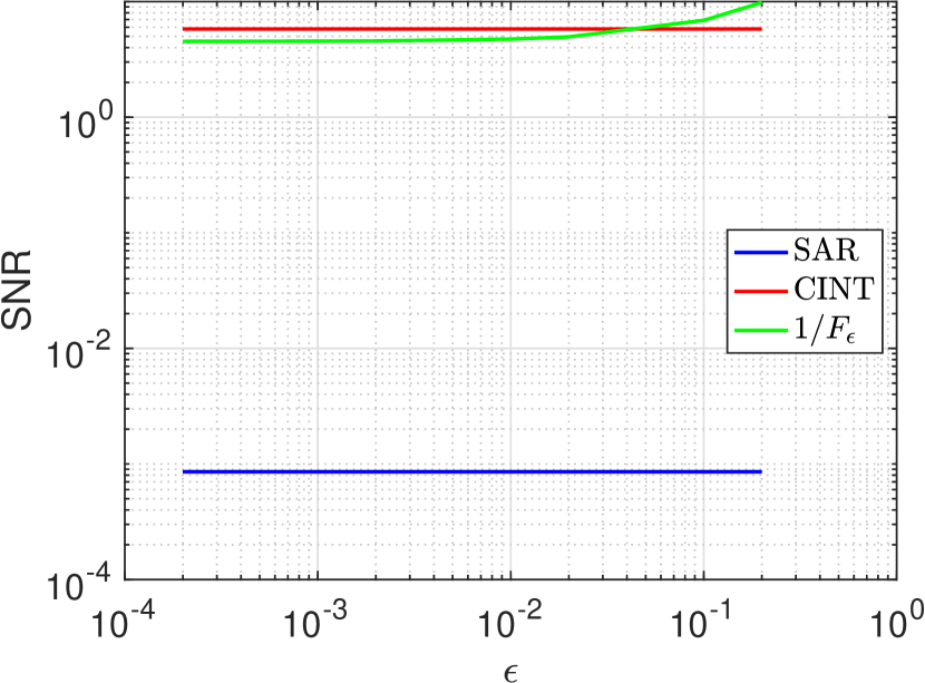
(a) $\tilde{\sigma}=0.4$

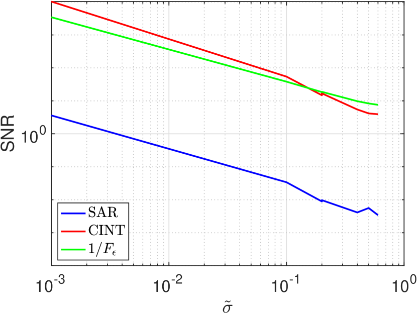
(b) $\epsilon=0.2$

Figure 14. Stability of the image as a function of the parameter $\epsilon$ with $\tilde{\sigma}=0.4$ (a) and as a function of $\tilde{\sigma}$ with $\epsilon=0.2$ (b). The CINT image is computed with $X_{d}=a/6$ and $\Omega_{d}=B/2$.

Following [3], we compute the image’s SNR defined as the mean of the image divided by its standard deviation in a small area around the true target location to estimate the stability of the imaging method. The sample mean and the sample standard deviation are computed using 100 realizations of the random medium with the same characteristics (correlation length and strength of fluctuations). For comparison, we also compute this SNR for the classical SAR image and the CINT image. The CINT method requires specifying two key parameters, the decoherence length $X_{d}$ and the decoherence frequency $\Omega_{d}$. In the CINT results that follow, we have set $X_{d}=a/6$ and $\Omega_{d}=B/2$. The results of these comparisons are shown in Fig. 14 where we compare SNR as a function of $\epsilon$ with $\tilde{\sigma}=0.4$ (Fig. 14(a)) and as a function of $\tilde{\sigma}$ with $\epsilon=0.2$ (Fig. 14(b)). Figure 14(a) and (b) illustrate the well-known result that classical SAR imaging results are statistically unstable in random media [3] since this SNR is very low. These results also suggest similar stability for CINT and $1/F_{\epsilon}$, both with comparably large SNRs. In Fig. 14(a), neither classical SAR nor CINT depend on $\epsilon$, so we see no change in behavior. However, as $\epsilon$ increases relative to $\tilde{\sigma}$ such that $\tilde{\sigma}/\sqrt{\epsilon}$ becomes small, we find that the SNR for $1/F_{\epsilon}$ becomes larger than that for CINT. In Fig. 14(b), all images decrease in SNR as $\tilde{\sigma}$ increases. However, the SNR for the CINT and $1/F_{\epsilon}$ images is three orders of magnitude higher than the one for classical SAR. It is important to note that the control offered by $\epsilon$ is limited because one cannot set the value of $\epsilon$ to be larger than $1$. Otherwise, one cannot separate the signal from the noise subspace.

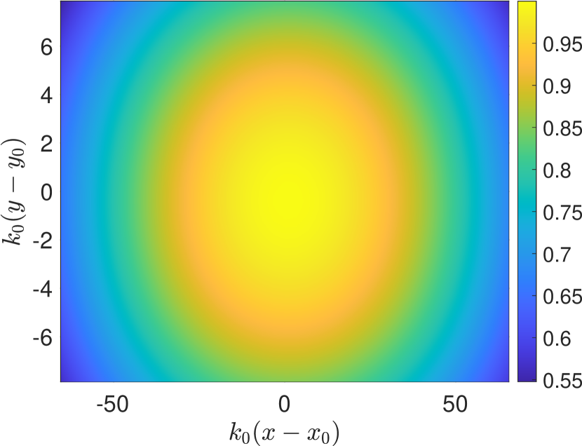
(a) CINT

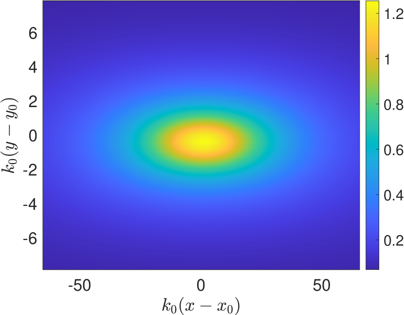
(b) $1/F_{\epsilon}$

Figure 15. Comparison of images formed using CINT with $X_{d}=a/6$ and $\Omega_{d}=B/2$ (a), and $1/F_{\epsilon}$ with $\epsilon$ and $\tilde{\sigma}$ satisfying $\tilde{\sigma}/\sqrt{\epsilon}=\sqrt{\epsilon}$.

Although the images formed using CINT and $1/F_{\epsilon}$ have similar stability behaviors, the image of $1/F_{\epsilon}$ has a much better resolution. In Fig. 15 we compare images formed using CINT and $1/F_{\epsilon}$ with $\epsilon$ and $\tilde{\sigma}$ set so that $\tilde{\sigma}/\sqrt{\epsilon}=\sqrt{\epsilon}$. These results show that the image formed by $1/F_{\epsilon}$ is focused more tightly on the target location in comparison to the image formed by CINT. Additionally, there is quantitative information available from the image formed by $1/F_{\epsilon}$. This tighter focus is especially true for range although resolution is also better with cross-range.

To see the effect of this improved resolution, we compare images formed using CINT and $1/F_{\epsilon}$ when the imaging region contains four point targets situated closely to one another in Fig. 16. For all of these images, $\tilde{\sigma}=0.2$. Figures 16(b) and (c) are formed using $1/F_{\epsilon}$ with $\epsilon=0.01$ and $0.001$, respectively. Here, the resolution of the CINT image does not allow for identification of the four targets. The $1/F_{\epsilon}$ with $\epsilon=0.01$ image has a sharper resolution, but allows for identification only three of the four targets. In contrast, the $1/F_{\epsilon}$ image with $\epsilon=0.001$ shows four distinct peaks indicating the target locations. These results show the potential importance of being able to tune the resolution of an image by varying the parameter $\epsilon$, even with random perturbations to the travel times.

8. Conclusions

We have introduced and analyzed a quantitative signal subspace imaging method for multi-frequency SAR measurements. The key to this method involves a simple rearrangement of the frequency data at each spatial location along the flight path where measurements are taken using the Prony method. Using this rearranged frequency data, this method involves two stages corresponding to two explicit imaging functionals, (12) and (14).

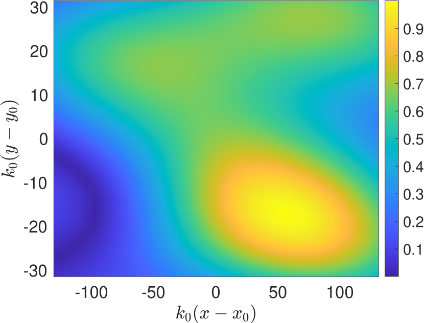
(a) CINT

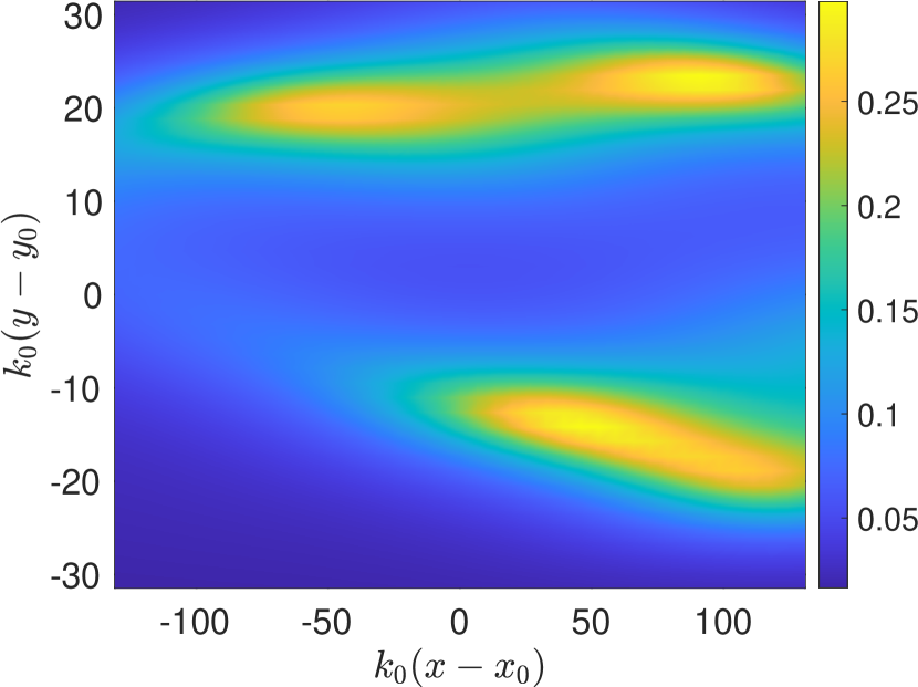
(b) $1/F_{\epsilon}$ with $\epsilon=0.01$

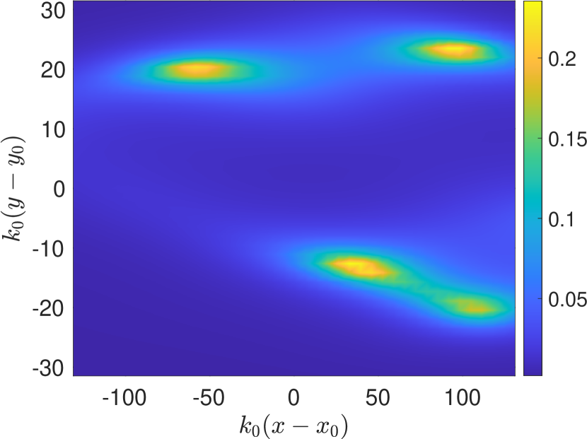
(c) $1/F_{\epsilon}$ with $\epsilon=0.001$

Figure 16. Comparison of images formed using CINT (a) and $1/F_{\epsilon}$ with $\epsilon=0.01$ (b) and $\epsilon=0.001$ (c) for four point targets. The CINT image is computed with $X_{d}=a/6$ and $\Omega_{d}=B/2$. The strength of the fluctuations is $\tilde{\sigma}=0.2$.

Images produced through evaluation of $1/F_{\epsilon}(\boldsymbol{y})$ over an imaging region attain tunably high-resolution images of target locations through a user-defined parameter $\epsilon$. Through a resolution analysis for a linear flight path, we have determined that the cross-range resolution of this imaging method is $O(\sqrt{\epsilon}(c/B)(L/a))$ where $c$ is the wave speed, $B$ is the bandwidth, $L$ is the distance from the center of the flight path to the center of the imaging region, and $a$ is the length of the synthetic aperture. We have also determined that the resolution of this imaging method in range is $O(\sqrt{\epsilon}(c/B)(L/R))$ where $R$ is the range distance from the center of the flight path to the center of the imaging region. With these resolution estimates, we see how the user-defined parameter $\epsilon$ may be set to adjust the image resolution for different settings.

Images produced through evaluation of $1/R_{\epsilon}(\boldsymbol{y})$ over an imaging region do not reveal target locations. However, if the target location is known, $1/R_{\epsilon}(\boldsymbol{y})$ provides an accurate method for recovering the complex reflectivity of a target. Again, the user-defined parameter $\epsilon$ can be set to regularize the function to enable stable recovery of the complex reflectivity. It is for this reason that we have proposed a two-stage imaging method in which $1/F_{\epsilon}(\boldsymbol{y})$ is used to determine location of target(s), and $1/R_{\epsilon}(\boldsymbol{y})$ is evaluated at those locations to recover the complex reflectivities. Additionally, the value of $\epsilon$ used for evaluating $1/F_{\epsilon}$ need not be the same used for evaluating $1/R_{\epsilon}$, so this parameter can be tuned independently for these two different imaging functionals.

When there is uncertainty in the travel times, we have shown that images formed by evaluating $1/F_{\epsilon}(\boldsymbol{y})$ have an expected value that is the same as the image formed in a homogeneous medium provided that the variances of the random perturbations are sufficiently small. Moreover, the variance of the image will be small for that case indicating that this imaging method is statistically stable to random perturbations in the travel times.

Both $F_{\epsilon}(\boldsymbol{y})$ and $R_{\epsilon}(\boldsymbol{y})$ are computed using the SVD of the rearranged data. Consequently, their effectiveness is understood to be related to how well the singular values corresponding to signals scattered by the targets are separated from noise. Provided that there is sufficient SNR for these singular values to be separated, the parameter $\epsilon$ mitigates noise and allows the user to control image resolution. When there is uncertainty in travel times, one can set the value of $\epsilon$ to ensure image accuracy and statistical stability which, in turn, will set the achievable image resolution.

Because this imaging method involves only elementary computations on the data and allows for user-control to produce high-resolution, quantitative images of targets, we believe that it is useful for a broad variety of SAR imaging applications.

References

- [1] R. Baraniuk and P. Steeghs, Compressive radar imaging, in 2007 IEEE Radar Conference, IEEE, 2007, pp. 128–133.
- [2] L. Borcea and J. Garnier, High-resolution interferometric synthetic aperture imaging in scattering media, SIAM J. Imaging Sci., 13 (2020), pp. 291–316.
- [3] L. Borcea, J. Garnier, G. Papanicolaou, and C. Tsogka, Enhanced statistical stability in coherent interferometric imaging, Inverse Probl., 27 (2011), p. 085004.
- [4] L. Borcea, M. Moscoso, G. Papanicolaou, and C. Tsogka, Synthetic aperture imaging of direction-and frequency-dependent reflectivities, SIAM J. Imaging Sci., 9 (2016), pp. 52–81.
- [5] C. H. Casteel Jr, L. A. Gorham, M. J. Minardi, S. M. Scarborough, K. D. Naidu, and U. K. Majumder, A challenge problem for 2d/3d imaging of targets from a volumetric data set in an urban environment, in Algorithms for Synthetic Aperture Radar Imagery XIV, vol. 6568, International Society for Optics and Photonics, 2007, p. 65680D.
- [6] M. Cheney, A mathematical tutorial on synthetic aperture radar, SIAM Review, 43 (2001), pp. 301–312.
- [7] M. Cheney and B. Borden, Fundamentals of Radar Imaging, vol. 79, SIAM, 2009.
- [8] A. J. Devaney, E. A. Marengo, and F. K. Gruber, Time-reversal-based imaging and inverse scattering of multiply scattering point targets, J. Acoust. Soc. Am., 118 (2005), pp. 3129–3138.
- [9] A. C. Fannjiang, The MUSIC algorithm for sparse objects: a compressed sensing analysis, Inverse Probl., 27 (2011), p. 035013.
- [10] J. Garnier and K. Solna, Coherent interferometric imaging for synthetic aperture radar in the presence of noise, Inverse Probl., 24 (2008), p. 055001.
- [11] P. González-Rodríguez, A. D. Kim, and C. Tsogka, Quantitative signal subspace imaging, Inverse Probl., (2021).
- [12] R. Griesmaier and C. Schmiedecke, A multifrequency MUSIC algorithm for locating small inhomogeneities in inverse scattering, Inverse Probl., 33 (2017), p. 035015.
- [13] D. Malioutov, M. Cetin, and A. Willsky, A sparse signal reconstruction perspective for source localization with sensor arrays, IEEE Trans. Signal Process., 53 (2005), pp. 3010–3022.
- [14] A. Moreira, P. Prats-Iraola, M. Younis, G. Krieger, I. Hajnsek, and K. P. Papathanassiou, A tutorial on synthetic aperture radar, IEEE Geosci. Remote Sens. Mag., 1 (2013), pp. 6–43.
- [15] M. Moscoso, A. Novikov, G. Papanicolaou, and C. Tsogka, Multifrequency interferometric imaging with intensity-only measurements, SIAM J. Imaging Sci., 10 (2017), pp. 1005–1032.
- [16] M. Moscoso, A. Novikov, G. Papanicolaou, and C. Tsogka, Robust multifrequency imaging with music, Inverse Probl., 35 (2019), p. 015007.
- [17] L. C. Potter, E. Ertin, J. T. Parker, and M. Cetin, Sparsity and compressed sensing in radar imaging, Proc. IEEE, 98 (2010), pp. 1006–1020.
- [18] G. R. B. Prony, Essai experimental et analytique sur les lois de la dilatalrlite de fluids elastiques et sur cells de la vapeur de l’alcool, à différents tempoeratures, J. de l’Ecole Polytech., 1 (1795), pp. 24–76.