Gravitational waveforms for compact binaries from second-order self-force theory
Abstract
We produce gravitational waveforms for nonspinning compact binaries undergoing a quasicircular inspiral. Our approach is based on a two-timescale expansion of the Einstein equations in second-order self-force theory, which allows first-principles waveform production in tens of milliseconds. Although the approach is designed for extreme mass ratios, our waveforms agree remarkably well with those from full numerical relativity, even for comparable-mass systems. Our results will be invaluable in accurately modelling extreme-mass-ratio inspirals for the LISA mission and intermediate-mass-ratio systems currently being observed by the LIGO-Virgo-KAGRA Collaboration.
Introduction. The era of gravitational-wave astronomy is upon us, with the LIGO-Virgo-KAGRA (LVK) Collaboration now routinely observing dozens of gravitational wave signals. In its most recent release, LVK announced the detection of 35 signals from the merger of compact-object binaries seen during the second half of its most recent observing run [1].
The majority of signals observed by LVK to date have been well represented by existing modelling approaches including numerical relativity (NR) [2], post-Newtonian (PN) theory [3], the effective one-body (EOB) formalism [4, 5, 6, 7], NR surrogates [8, 9], and phenomenological models [10, 11, 12]. However, LVK is now beginning to see glimpses of binary systems that push the limits of those approaches. One signal, GW191219_163120, thought to have come from the merger of a mass ratio binary, was outside the region of parameter space where existing models have been validated, and LVK concluded that there may be systematic uncertainties in their results for that signal as a consequence [1].
In parallel to the efforts of the LVK Collaboration, members of the LISA Consortium are preparing for the space-based Laser Interferometer Space Antenna [13], which will be sensitive to low-frequency, millihertz gravitational wave signals outside of the LVK sensitivity band. LISA will observe new categories of sources including supermassive black hole binaries—involving a pair of comparable-mass supermassive black holes—and extreme-mass-ratio inspirals (EMRIs)—consisting of a stellar-mass compact object in orbit around a supermassive black hole [14]. EMRIs, in particular, are expected to be well outside the range of mass ratios and orbital configurations accessible to existing waveform models used by the LVK Collaboration.
The primary method of modelling EMRIs is the gravitational self-force approach [15, 16], which solves the Einstein field equations using an expansion in powers of the mass ratio , where and are the binary’s constituent masses. At zeroth order in , the companion moves on a geodesic of the primary’s spacetime, and at higher orders it experiences a self-force that drives its inspiral. It is widely expected [17, 18] that this expansion must be carried to second order in to achieve the necessary accuracy for LISA. That expectation is motivated by the fact that over an inspiral, the gravitational waveform phase has an expansion of the form [19, 16]
| (1) |
The “adiabatic” (0PA) term involves dissipative effects of the first-order self-force (along with geodesic effects), and the “first post-adiabatic” (1PA) term involves dissipative effects of the second-order self-force (along with first-order conservative effects). The 1PA contribution to Eq. (1) is nonnegligible for all mass ratios, but the error term (which would involve third-and-higher-order effects) is negligible for sufficiently small , suggesting that second order is both necessary and sufficient for EMRI modelling. Recent estimates have suggested 1PA models may even suffice to cover much of the non-extreme binary parameter space [20, 21], further motivating the pursuit of such models.
In this Letter we present the first-ever calculation of these 1PA waveforms by solving the Einstein equations through second order in the mass ratio for nonspinning binaries in quasicircular orbits. Our model also performs remarkably well for more comparable mass ratios – see Fig. 1 – which broadly validates the predictions of Ref. [20].
Our model assumes the larger body is a nonspinning black hole, while its companion can be any (nonspinning) compact object. We use geometrized units with . We also define the large mass ratio and symmetric mass ratio , where is the total mass. Our method begins from expansions in powers of at fixed , but we consistently re-expand our results in powers of at fixed . This restores in the perturbative solution the inherent discrete symmetry of the full solution under the interchange of the two bodies [23], and yields the most accurate results in the comparable-mass regime [24, 25, 26, 27, 28, 29, 30, 31, 32, 33, 20].
Two-timescale expansion. We utilize the second-order self-force framework developed in Refs. [34, 35, 36, 37, 38, 39, 40, 41, 42, 43, 44, 45], building particularly on the two-timescale expansion in Ref. [42] and the results reported in [46, 47]. A detailed explanation of our model is given in Ref. [48], so we restrict ourselves here to a summary of the most pertinent points. The model treats as a small parameter, decomposing the spacetime metric as , where is the Schwarzschild metric of the large black hole and . The perturbation is expanded through order in terms of slowly evolving amplitudes and oscillatory phase factors ,
| (2) |
where are spatial coordinates.
All time dependence is encoded in the parameters —the black hole’s mass and the companion’s orbital frequency —and in the orbital phase . slowly evolves due to gravitational-wave emission and absorption; in this evolution, an PA approximation includes all terms contributing through order .
The amplitudes are determined by using separation of variables to decompose the first- and second-order Einstein equations into radial ordinary differential equations for the spherical-harmonic modes of [37, 38, 42]. After solving on a grid of values and storing , we can rapidly generate waveforms by solving evolution equations for and and evaluating Eq. (2) at future null infinity.
1PA equations of motion. Although the evolution of (and of the black hole’s spin, which slowly grows to ) formally appears at 1PA order, the effects are numerically subdominant [49] so we choose to neglect them. We thus only need to consider the evolution of the orbital frequency, . We determine an equation for by employing an energy balance law, combining the results of [46, 47] for the flux of gravitational-wave energy to infinity and the binding energy . Taking a time derivative of and rearranging, we obtain a set of orbital evolution equations,
| (3) |
where , and is the standard leading-order energy flux into the black hole [50, 51, 52]; other than this contribution to the balance law, ’s evolution is a strictly 1PA effect, and we henceforth treat as constant. A full discussion of Eq. (3) and its neglect of numerically small 1PA effects can be found in Sec. IIB of Ref. [48].
The flux and binding energy are computed from the amplitudes [46, 47]. We expand them in powers of at fixed as [47] and [46], where is a dimensionless measure of the inverse separation, , and . The self-force contribution to the binding energy is evaluated using the prediction from the first law of compact binary mechanics [53, 29], which provides an excellent approximation over the entire inspiral phase [46]. Here and below, a numerical superscript indicates a quantity computed from up to , while a numerical subscript denotes the PA order at which a quantity contributes. Fully expanding Eq. (3) in powers of , we then arrive at our first time-domain post-adiabatic (1PAT1) model for the orbital evolution,
| (4) |
where and , with and .
Eq. (4) can be rapidly integrated to generate a trajectory, but the 1PAT1 model has the disadvantage of requiring the mass ratio to be chosen before solving the equations of motion. An even more efficient approach is to expand the orbital phase and frequency as and , where . Substituting this into Eq. (4) and re-expanding, we obtain a second time-domain post-adiabatic model (1PAT2), comprising a hierarchical sequence of equations in which the dependence on the mass ratio has been fully factored out,
| (5a) | |||
| (5b) | |||
where . These can be integrated in advance, and their solutions stored, without specifying a mass ratio. Trajectories can then be immediately generated for any given mass ratio.
Although 1PAT2 has an advantage in terms of computational efficiency, comparisons with NR reveal that 1PAT1 has a distinct advantage in terms of accuracy. This is typical of asymptotic methods: expansions at fixed values of determinative dynamical variables ( in this case) are more accurate than expansions at fixed values of extrinsic time parameters ( in this case). The 1PAT2 model also breaks down earlier in the inspiral than 1PAT1, as it directly involves the relationship of an adiabatic model (0PA, given by the equations for and alone), which for comparable-mass binaries becomes singular significantly earlier than the 1PAT1 model.
In addition to time-domain waveforms, the two-timescale approach naturally lends itself to the production of frequency-domain waveforms. Writing , substituting in the 1PAT1 equations for , and re-expanding in , we arrive at a frequency-domain post-adiabatic (1PAF1) model: , where
| (6) |
This combines the accuracy advantage of 1PAT1 with the efficiency advantage of 1PAT2. Moreover, frequency-domain waveforms can be especially convenient for data analysis purposes [54].
Waveform. In order to extract a waveform from our post-adiabatic models we write the strain in terms of a certain tetrad component of our metric perturbation, where . Decomposing into spin-weight spherical harmonic modes and expanding in the symmetric mass ratio yields
| (7) |
where is the asymptotic amplitude from Eq. (2) [i.e., the mode of ], evaluated at . In 1PAT2, the amplitudes are further expanded as .
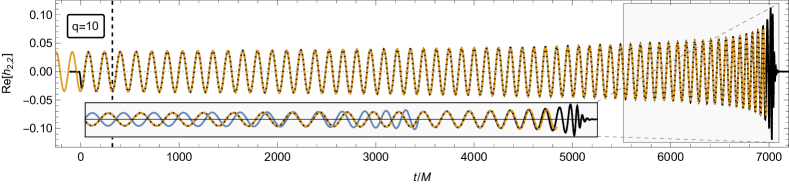
Results. In Fig. 1 we plot the real part of the 1PAT1 waveform for a mass ratio binary (similar plots for mass ratios , , and , as well as a comparison with a post-Newtonian waveform, are given as supplemental material [55]). Our waveform (orange) agrees remarkably well with an equivalent waveform produced using an NR simulation (black) until very close to merger, at which point the assumption of adiabaticity breaks down. In contrast, a 0PA waveform (shown in blue in the inset) produced using only the leading-order-in- contributions falls badly out of phase much earlier.
Decomposing the complex waveform modes into a (real) amplitude and phase, we see from Figs. 2 and 3 that both are well captured by our model. This conclusion holds not only for the dominant mode, but also for higher modes. For the mode with we find that the phase error is less than radians and the amplitude error is essentially unmeasurable (i.e. is less than uncertainties in the NR simulation) until waveform cycles before merger.
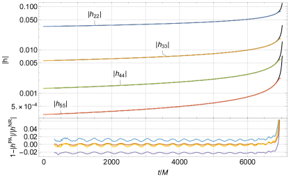
The bottom panel of Fig. 2 shows that the odd- mode amplitudes agree slightly less well with NR results. This can be traced to our perturbative solution’s failure to capture the inherent discrete antisymmetry of the odd- modes under the interchange of the two bodies, as is fully explicit in PN waveforms [3, 56]. We can restore that antisymmetry by multiplying and dividing by , re-expanding the denominator, and truncating at order to obtain amplitudes . This “resummation” yields the small but appreciable improvement in accuracy seen in the bottom panel of Fig. 2. (However, we stress that no resummations are used in any other figures.)
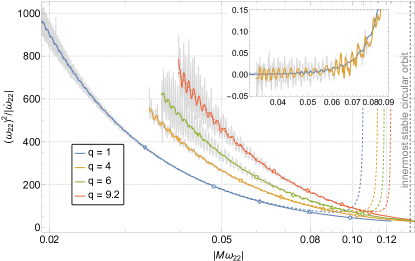
As an alternative to computing the phase difference as a function of time as a measure of accuracy of our waveform, it is useful to compute the dimensionless adiabaticity parameter or its inverse [57]. When this parameter becomes large, the orbit is evolving rapidly and our adiabatic assumption breaks down. The integral of its inverse, , with respect to yields the accumulated phase so this is an indirect measure of the phase accuracy of our waveforms. By plotting the adiabaticity parameter as a function of waveform frequency, , we completely eliminate the sensitive dependence of the comparison on any particular choice of point at which to align the phase and frequency of two waveforms. Figure 4 shows the inverse adiabaticity parameter computed in NR and the 1PAT1 model as a function of (on a logarithmic scale) for a range of mass ratios. We see that NR and 1PAT1 agree very well until just a few waveform cycles before merger, at which point the adiabatic assumption has broken down and we have no reason to trust our two-timescale models.
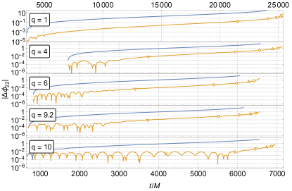
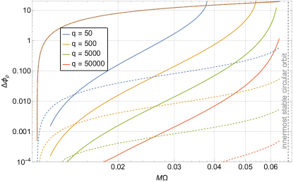
We can also internally assess the accuracy of our models by comparing each of our three models for the orbital phase (0PA, 1PAT1, and 1PAT2). Figure 5 shows the result of this comparison for a range of small mass ratios that are outside the reach of current NR simulations. Although these do not tell us about the absolute error in our models, the comparison does solidify the notion that 0PA waveforms are totally inadequate. So-called “kludge” models often used for EMRI data analysis [62] are even less accurate, as they represent approximations to the 0PA waveform. Our faster 1PAT2 model agrees modestly well with the 1PAT1 model, with the agreement improving with mass ratio, as expected given that the difference between the models is . However, if one is interested in phase accuracy within a fraction of a radian close to the test-particle innermost stable circular orbit (ISCO), it is clear that the 1PAT2 model will only be useful in that case for .
Finally, we highlight the speed of waveform generation within our setup. The functions on the right-hand side of the 1PA equations of motion are non-oscillatory and, as such, the ordinary differential equations in Eqs. (4)-(6) can be numerically integrated very rapidly, on the order of milliseconds. The waveform is then constructed by evaluating Eq. (7) at the relevant sample times and summing over spherical harmonic modes. It was recently shown that for waveforms containing orders of magnitude more modes than appear in our quasi-circular setup this summation and sampling step can be performed in a 0PA model in few hundred milliseconds for, e.g., year-long EMRI waveforms containing time steps [63, 64]. The structure of the equations at 1PA is the same as at 0PA, so 1PA waveform generation is just as rapid.
Conclusions. The waveforms computed in this work represent the first major result in a programme to produce post-adiabatic waveforms for compact binaries. Although restricted to the case of nonspinning systems and quasicircular orbits, it is nonetheless likely that these waveforms will be useful in their own right. The LVK Collaboration has begun to observe systems with mass ratios well outside the comfort zone of existing waveform models [1], while at the same time being well within the range of validity of our post-adiabatic model.
There are several natural future directions in which to take this work. These primarily revolve around treating more generic configurations, for example where one or both of the compact objects are spinning, or where the orbit may be eccentric and/or precessing. Another important area of improvement is the treatment of the very last stages of the waveform. Our adiabaticity assumption breaks down as the system approaches the ISCO, where we must transition to a plunge model [65, 66, 67, 68] followed by a quasinormal mode ringdown [69].
Improvements might also be made to our 1PA inspiral model. We have three sources of uncertainty in our 1PA evolution equations: our use of the first-law binding energy, our neglect of 1PA effects of the primary black hole’s evolution, and our neglect of the 1PA horizon absorption . These are analyzed in detail in Ref. [48]. While their impact is small, it is potentially nonnegligible. In future work we will eliminate them by using the second-order dissipative self-force and the full set of 1PA evolution equations [42].
Acknowledgements.
Acknowledgements. We thank Alessandro Nagar and Angelica Albertini for comments on an early draft of this letter. AP acknowledges support from a Royal Society University Research Fellowship, a Royal Society Research Fellows Enhancement Award, and a Royal Society Research Grant for Research Fellows. NW acknowledges support from a Royal Society - Science Foundation Ireland University Research Fellowship via grants UF160093 and RGF\R1\180022. This work makes use of the Black Hole Perturbation Toolkit [52] and Simulation Tools [70].References
- Abbott et al. [2021] R. Abbott et al. (LIGO Scientific, VIRGO, KAGRA), GWTC-3: Compact Binary Coalescences Observed by LIGO and Virgo During the Second Part of the Third Observing Run, (2021), arXiv:2111.03606 [gr-qc] .
- Duez and Zlochower [2019] M. D. Duez and Y. Zlochower, Numerical Relativity of Compact Binaries in the 21st Century, Rept. Prog. Phys. 82, 016902 (2019), arXiv:1808.06011 [gr-qc] .
- Blanchet [2014] L. Blanchet, Gravitational Radiation from Post-Newtonian Sources and Inspiralling Compact Binaries, Living Rev. Rel. 17, 2 (2014), arXiv:1310.1528 [gr-qc] .
- Ossokine et al. [2020] S. Ossokine et al., Multipolar Effective-One-Body Waveforms for Precessing Binary Black Holes: Construction and Validation, Phys. Rev. D 102, 044055 (2020), arXiv:2004.09442 [gr-qc] .
- Nagar et al. [2018] A. Nagar et al., Time-domain effective-one-body gravitational waveforms for coalescing compact binaries with nonprecessing spins, tides and self-spin effects, Phys. Rev. D 98, 104052 (2018), arXiv:1806.01772 [gr-qc] .
- Cotesta et al. [2018] R. Cotesta, A. Buonanno, A. Bohé, A. Taracchini, I. Hinder, and S. Ossokine, Enriching the Symphony of Gravitational Waves from Binary Black Holes by Tuning Higher Harmonics, Phys. Rev. D 98, 084028 (2018), arXiv:1803.10701 [gr-qc] .
- Cotesta et al. [2020] R. Cotesta, S. Marsat, and M. Pürrer, Frequency domain reduced order model of aligned-spin effective-one-body waveforms with higher-order modes, Phys. Rev. D 101, 124040 (2020), arXiv:2003.12079 [gr-qc] .
- Varma et al. [2019a] V. Varma, S. E. Field, M. A. Scheel, J. Blackman, L. E. Kidder, and H. P. Pfeiffer, Surrogate model of hybridized numerical relativity binary black hole waveforms, Phys. Rev. D 99, 064045 (2019a), arXiv:1812.07865 [gr-qc] .
- Varma et al. [2019b] V. Varma, S. E. Field, M. A. Scheel, J. Blackman, D. Gerosa, L. C. Stein, L. E. Kidder, and H. P. Pfeiffer, Surrogate models for precessing binary black hole simulations with unequal masses, Phys. Rev. Research. 1, 033015 (2019b), arXiv:1905.09300 [gr-qc] .
- Pratten et al. [2020] G. Pratten, S. Husa, C. Garcia-Quiros, M. Colleoni, A. Ramos-Buades, H. Estelles, and R. Jaume, Setting the cornerstone for a family of models for gravitational waves from compact binaries: The dominant harmonic for nonprecessing quasicircular black holes, Phys. Rev. D 102, 064001 (2020), arXiv:2001.11412 [gr-qc] .
- Pratten et al. [2021] G. Pratten et al., Computationally efficient models for the dominant and subdominant harmonic modes of precessing binary black holes, Phys. Rev. D 103, 104056 (2021), arXiv:2004.06503 [gr-qc] .
- García-Quirós et al. [2020] C. García-Quirós, M. Colleoni, S. Husa, H. Estellés, G. Pratten, A. Ramos-Buades, M. Mateu-Lucena, and R. Jaume, Multimode frequency-domain model for the gravitational wave signal from nonprecessing black-hole binaries, Phys. Rev. D 102, 064002 (2020), arXiv:2001.10914 [gr-qc] .
- Amaro-Seoane et al. [2017] P. Amaro-Seoane et al. (LISA), Laser Interferometer Space Antenna, (2017), arXiv:1702.00786 [astro-ph.IM] .
- Babak et al. [2017] S. Babak, J. Gair, A. Sesana, E. Barausse, C. F. Sopuerta, C. P. L. Berry, E. Berti, P. Amaro-Seoane, A. Petiteau, and A. Klein, Science with the space-based interferometer LISA. V: Extreme mass-ratio inspirals, Phys. Rev. D 95, 103012 (2017), arXiv:1703.09722 .
- Barack and Pound [2019] L. Barack and A. Pound, Self-force and radiation reaction in general relativity, Rept. Prog. Phys. 82, 016904 (2019), arXiv:1805.10385 [gr-qc] .
- Pound and Wardell [2021] A. Pound and B. Wardell, Black hole perturbation theory and gravitational self-force, (2021), arXiv:2101.04592 [gr-qc] .
- Arun et al. [2022] K. G. Arun et al. (LISA), New horizons for fundamental physics with LISA, Living Rev. Rel. 25, 4 (2022), arXiv:2205.01597 [gr-qc] .
- Amaro-Seoane et al. [2022] P. Amaro-Seoane et al., Astrophysics with the Laser Interferometer Space Antenna, (2022), arXiv:2203.06016 [gr-qc] .
- Hinderer and Flanagan [2008] T. Hinderer and E. E. Flanagan, Two timescale analysis of extreme mass ratio inspirals in Kerr. I. Orbital Motion, Phys. Rev. D 78, 064028 (2008), arXiv:0805.3337 [gr-qc] .
- van de Meent and Pfeiffer [2020] M. van de Meent and H. P. Pfeiffer, Intermediate mass-ratio black hole binaries: Applicability of small mass-ratio perturbation theory, Phys. Rev. Lett. 125, 181101 (2020), arXiv:2006.12036 [gr-qc] .
- Ramos-Buades et al. [2022] A. Ramos-Buades, M. van de Meent, H. P. Pfeiffer, H. R. Rüter, M. A. Scheel, M. Boyle, and L. E. Kidder, Eccentric binary black holes: Comparing numerical relativity and small mass-ratio perturbation theory, (2022), arXiv:2209.03390 [gr-qc] .
- SXS Collaboration [2019a] SXS Collaboration, Binary black-hole simulation SXS:BBH:1107 (2019a).
- Le Tiec [2014] A. Le Tiec, The Overlap of Numerical Relativity, Perturbation Theory and Post-Newtonian Theory in the Binary Black Hole Problem, Int. J. Mod. Phys. D 23, 1430022 (2014), arXiv:1408.5505 .
- Fitchett and Detweiler [1984] M. J. Fitchett and S. L. Detweiler, Linear momentum and gravitational-waves - circular orbits around a schwarzschild black-hole, Mon. Not. Roy. Astron. Soc. 211, 933 (1984).
- Anninos et al. [1995] P. Anninos, D. Hobill, E. Seidel, L. Smarr, and W.-M. Suen, The Headon collision of two equal mass black holes, Phys. Rev. D 52, 2044 (1995), arXiv:gr-qc/9408041 .
- Favata et al. [2004] M. Favata, S. A. Hughes, and D. E. Holz, How black holes get their kicks: Gravitational radiation recoil revisited, Astrophys. J. Lett. 607, L5 (2004), arXiv:astro-ph/0402056 .
- Sperhake et al. [2011] U. Sperhake, V. Cardoso, C. D. Ott, E. Schnetter, and H. Witek, Extreme black hole simulations: collisions of unequal mass black holes and the point particle limit, Phys. Rev. D 84, 084038 (2011), arXiv:1105.5391 [gr-qc] .
- Le Tiec et al. [2011] A. Le Tiec, A. H. Mroue, L. Barack, A. Buonanno, H. P. Pfeiffer, N. Sago, and A. Taracchini, Periastron Advance in Black Hole Binaries, Phys. Rev. Lett. 107, 141101 (2011), arXiv:1106.3278 [gr-qc] .
- Le Tiec et al. [2012a] A. Le Tiec, E. Barausse, and A. Buonanno, Gravitational Self-Force Correction to the Binding Energy of Compact Binary Systems, Phys. Rev. Lett. 108, 131103 (2012a), arXiv:1111.5609 .
- Le Tiec et al. [2013] A. Le Tiec et al., Periastron Advance in Spinning Black Hole Binaries: Gravitational Self-Force from Numerical Relativity, Phys. Rev. D 88, 124027 (2013), arXiv:1309.0541 [gr-qc] .
- Nagar [2013] A. Nagar, Gravitational recoil in nonspinning black hole binaries: the span of test-mass results, Phys. Rev. D 88, 121501 (2013), arXiv:1306.6299 [gr-qc] .
- Le Tiec and Grandclément [2018] A. Le Tiec and P. Grandclément, Horizon Surface Gravity in Corotating Black Hole Binaries, Class. Quant. Grav. 35, 144002 (2018), arXiv:1710.03673 [gr-qc] .
- Rifat et al. [2020] N. E. M. Rifat, S. E. Field, G. Khanna, and V. Varma, Surrogate model for gravitational wave signals from comparable and large-mass-ratio black hole binaries, Phys. Rev. D 101, 081502 (2020), arXiv:1910.10473 [gr-qc] .
- Pound [2012a] A. Pound, Second-order gravitational self-force, Phys. Rev. Lett. 109, 051101 (2012a), arXiv:1201.5089 .
- Pound [2012b] A. Pound, Nonlinear gravitational self-force: Field outside a small body, Phys. Rev. D 86, 084019 (2012b), arXiv:1206.6538 .
- Pound and Miller [2014] A. Pound and J. Miller, A practical, covariant puncture for second-order self-force calculations, Phys. Rev. D 89, 104020 (2014), arXiv:1403.1843 .
- Warburton and Wardell [2014] N. Warburton and B. Wardell, Applying the effective-source approach to frequency-domain self-force calculations, Phys. Rev. D 89, 044046 (2014), arXiv:1311.3104 .
- Wardell and Warburton [2015] B. Wardell and N. Warburton, Applying the effective-source approach to frequency-domain self-force calculations: Lorenz-gauge gravitational perturbations, Phys. Rev. D 92, 084019 (2015), arXiv:1505.07841 .
- Pound [2015] A. Pound, Second-order perturbation theory: problems on large scales, Phys. Rev. D 92, 104047 (2015), arXiv:1510.05172 .
- Miller et al. [2016] J. Miller, B. Wardell, and A. Pound, Second-order perturbation theory: the problem of infinite mode coupling, Phys. Rev. D 94, 104018 (2016), arXiv:1608.06783 .
- Pound [2017] A. Pound, Nonlinear gravitational self-force: second-order equation of motion, Phys. Rev. D 95, 104056 (2017), arXiv:1703.02836 .
- Miller and Pound [2021] J. Miller and A. Pound, Two-timescale evolution of extreme-mass-ratio inspirals: waveform generation scheme for quasicircular orbits in Schwarzschild spacetime, Phys. Rev. D 103, 064048 (2021), arXiv:2006.11263 [gr-qc] .
- Spiers et al. [tion] A. Spiers, A. Pound, and B. Wardell, Second-order perturbation theory in Schwarzschild spacetime (in preparation).
- Miller et al. [tion] J. Miller, B. Leather, A. Pound, and N. Warburton, Frequency-domain methods for first- and second-order self-force calculations in Schwarzschild spacetime (in preparation).
- Durkan and Warburton [2022] L. Durkan and N. Warburton, Slow evolution of the metric perturbation due to a quasicircular inspiral into a Schwarzschild black hole, (2022), arXiv:2206.08179 [gr-qc] .
- Pound et al. [2020] A. Pound, B. Wardell, N. Warburton, and J. Miller, Second-Order Self-Force Calculation of Gravitational Binding Energy in Compact Binaries, Phys. Rev. Lett. 124, 021101 (2020), arXiv:1908.07419 [gr-qc] .
- Warburton et al. [2021] N. Warburton, A. Pound, B. Wardell, J. Miller, and L. Durkan, Gravitational-Wave Energy Flux for Compact Binaries through Second Order in the Mass Ratio, Phys. Rev. Lett. 127, 151102 (2021), arXiv:2107.01298 [gr-qc] .
- Albertini et al. [2022] A. Albertini, A. Nagar, A. Pound, N. Warburton, B. Wardell, L. Durkan, and J. Miller, Comparing second-order gravitational self-force, numerical relativity and effective one body waveforms from inspiralling, quasi-circular and nonspinning black hole binaries, (2022), arXiv:2208.01049 [gr-qc] .
- Martel [2004] K. Martel, Gravitational wave forms from a point particle orbiting a Schwarzschild black hole, Phys. Rev. D 69, 044025 (2004), arXiv:gr-qc/0311017 .
- Hughes [2000] S. A. Hughes, The Evolution of circular, nonequatorial orbits of Kerr black holes due to gravitational wave emission, Phys. Rev. D 61, 084004 (2000), [Erratum: Phys.Rev.D 63, 049902 (2001), Erratum: Phys.Rev.D 65, 069902 (2002), Erratum: Phys.Rev.D 67, 089901 (2003), Erratum: Phys.Rev.D 78, 109902 (2008), Erratum: Phys.Rev.D 90, 109904 (2014)], arXiv:gr-qc/9910091 .
- Fujita et al. [2009] R. Fujita, W. Hikida, and H. Tagoshi, An Efficient Numerical Method for Computing Gravitational Waves Induced by a Particle Moving on Eccentric Inclined Orbits around a Kerr Black Hole, Prog. Theor. Phys. 121, 843 (2009), arXiv:0904.3810 [gr-qc] .
- [52] Black Hole Perturbation Toolkit, (bhptoolkit.org).
- Le Tiec et al. [2012b] A. Le Tiec, L. Blanchet, and B. F. Whiting, The First Law of Binary Black Hole Mechanics in General Relativity and Post-Newtonian Theory, Phys. Rev. D 85, 064039 (2012b), arXiv:1111.5378 .
- Abbott et al. [2020] B. P. Abbott et al. (LIGO Scientific, Virgo), A guide to LIGO–Virgo detector noise and extraction of transient gravitational-wave signals, Class. Quant. Grav. 37, 055002 (2020), arXiv:1908.11170 [gr-qc] .
- [55] See Supplemental Material for additional plots comparing 1PAT1 waveforms against NR simulations [58, 59, 60, 61] for mass ratios , , and , as well as a comparison with a post-Newtonian waveform [71].
- Kidder [2008] L. E. Kidder, Using full information when computing modes of post-Newtonian waveforms from inspiralling compact binaries in circular orbit, Phys. Rev. D 77, 044016 (2008), arXiv:0710.0614 [gr-qc] .
- Baiotti et al. [2010] L. Baiotti, T. Damour, B. Giacomazzo, A. Nagar, and L. Rezzolla, Analytic modelling of tidal effects in the relativistic inspiral of binary neutron stars, Phys. Rev. Lett. 105, 261101 (2010), arXiv:1009.0521 [gr-qc] .
- SXS Collaboration [2019b] SXS Collaboration, Binary black-hole simulation SXS:BBH:1132 (2019b).
- SXS Collaboration [2019c] SXS Collaboration, Binary black-hole simulation SXS:BBH:1220 (2019c).
- SXS Collaboration [2019d] SXS Collaboration, Binary black-hole simulation SXS:BBH:0181 (2019d).
- SXS Collaboration [2019e] SXS Collaboration, Binary black-hole simulation SXS:BBH:1108 (2019e).
- Chua et al. [2017] A. J. K. Chua, C. J. Moore, and J. R. Gair, Augmented kludge waveforms for detecting extreme-mass-ratio inspirals, Phys. Rev. D 96, 044005 (2017), arXiv:1705.04259 [gr-qc] .
- Chua et al. [2021] A. J. K. Chua, M. L. Katz, N. Warburton, and S. A. Hughes, Rapid generation of fully relativistic extreme-mass-ratio-inspiral waveform templates for LISA data analysis, Phys. Rev. Lett. 126, 051102 (2021), arXiv:2008.06071 [gr-qc] .
- Katz et al. [2021] M. L. Katz, A. J. K. Chua, L. Speri, N. Warburton, and S. A. Hughes, Fast extreme-mass-ratio-inspiral waveforms: New tools for millihertz gravitational-wave data analysis, Phys. Rev. D 104, 064047 (2021), arXiv:2104.04582 [gr-qc] .
- Ori and Thorne [2000] A. Ori and K. S. Thorne, The Transition from inspiral to plunge for a compact body in a circular equatorial orbit around a massive, spinning black hole, Phys. Rev. D 62, 124022 (2000), arXiv:gr-qc/0003032 .
- Apte and Hughes [2019] A. Apte and S. A. Hughes, Exciting black hole modes via misaligned coalescences: I. Inspiral, transition, and plunge trajectories using a generalized Ori-Thorne procedure, Phys. Rev. D 100, 084031 (2019), arXiv:1901.05901 [gr-qc] .
- Burke et al. [2020] O. Burke, J. R. Gair, and J. Simón, Transition from Inspiral to Plunge: A Complete Near-Extremal Trajectory and Associated Waveform, Phys. Rev. D 101, 064026 (2020), arXiv:1909.12846 [gr-qc] .
- Compère and Küchler [2021] G. Compère and L. Küchler, Asymptotically matched quasi-circular inspiral and transition-to-plunge in the small mass ratio expansion, (2021), arXiv:2112.02114 [gr-qc] .
- Hatsuda and Kimura [2020] Y. Hatsuda and M. Kimura, Semi-analytic expressions for quasinormal modes of slowly rotating Kerr black holes, Phys. Rev. D 102, 044032 (2020), arXiv:2006.15496 [gr-qc] .
- [70] I. Hinder and B. Wardell, SimulationTools for Mathematica, http://simulationtools.org.
- Damour et al. [2001] T. Damour, B. R. Iyer, and B. S. Sathyaprakash, A Comparison of search templates for gravitational waves from binary inspiral, Phys. Rev. D 63, 044023 (2001), [Erratum: Phys.Rev.D 72, 029902 (2005)], arXiv:gr-qc/0010009 .