Entropy-Regularized Partially Observed
Markov Decision Processes
Abstract
We investigate partially observed Markov decision processes (POMDPs) with cost functions regularized by entropy terms describing state, observation, and control uncertainty. Standard POMDP techniques are shown to offer bounded-error solutions to these entropy-regularized POMDPs, with exact solutions possible when the regularization involves the joint entropy of the state, observation, and control trajectories. Our joint-entropy result is particularly surprising since it constitutes a novel, tractable formulation of active state estimation.
I Introduction
Partially observed Markov decision processes (POMDPs) and Markov decision processes (MDPs) with information-theoretic costs have attracted widespread attention across systems and control [2, 3, 4, 5], computer science [6, 7, 8], signal processing [9, 10, 11, 12], and robotics [13, 14, 15]. Interest in such POMDPs has been driven, in large part, by active state estimation problems in which information-theoretic costs describing the uncertainty about latent states are minimized in order to aid or enhance the performance of state estimation algorithms [9, 10, 6, 5]. Interest in such MDPs has, in contrast, been driven by a desire within applications such as networked control and economics to develop control policies (or decision-makers) that are rationally inattentive or “data-frugal” in that they trade-off control performance to reduce the (data) rate at which state information is used to make control decisions [2, 3, 8]. Despite interest in rate-cost trade-offs in MDPs, limited attention has been paid to similar problems in POMDPs. Motivated by data-frugal POMDPs with potential applications to active state estimation, we investigate POMDPs with information-theoretic entropy costs that penalize observation incompressibility and/or state uncertainty.
POMDPs with information-theoretic costs have been extensively investigated for active state estimation, with popular costs including the (negative) mutual information between states and observations [4], the (Shannon or Rényi) entropy of Bayesian filter estimates [9, 13, 6], and the entropy of Bayesian smoother or Viterbi algorithm estimates [14, 15, 5] (see [10, Chapter 8] and references therein for more). These POMDPs have been shown to be amenable to bounded-error (approximate) solution using standard POMDP solvers when their cost and cost-to-go (or value functions) are concave and admit piecewise-linear concave (PWLC) approximations (cf. [10, Section 8.4.4], [6]). For example, we recently showed that the smoother entropy (i.e., the conditional entropy of the state trajectory given observations and controls) can be (approximately) optimized in this manner [5, 16].
Outside of applications involving active state estimation, POMDPs with information-theoretic costs have received only limited specialized attention. Most notably, in Bayesian experimental design (involving degenerate POMDPs with a time-invariant or constant state), the entropy of the observations has been explored as a cost to encourage the selection of controls (i.e. experiments) with predictable outcomes (see [17, 18]). In the context of linear-quadratic regulators and linear-quadratic-Gaussian control (i.e. POMDPs with specialized linear dynamics but continuous state, control, and observation spaces), the directed information from the observations to controls has been used as a cost to study the trade-off between feedback (data) rates and control costs (see [19, 20, 21]). Similarly, in the context of MDPs (i.e. degenerate POMDPs with fully observed states), various information-theoretic quantities such as the directed information, mutual information, and transfer entropy, have been used as costs to penalize feedback from the states to the controls so as to study rate-cost trade-offs [2, 3, 8]. Despite growing interest, solving POMDPs (and MDPs) with rate-cost trade-offs has proved difficult due to complications including randomized policies [2, 19, 17, 18], the design of observation processes [2, 19, 3, 8], and the need to solve nonconvex optimization problems [2, 7].
The main contribution of this paper is the proposal of POMDPs with costs regularized by combinations of the input-output entropy (i.e. the entropy of the observations and controls) and the smoother entropy. Such entropy-regularized POMDPs (ERPOMDPs) are novel in that they both introduce rate-cost trade-offs into standard POMDPs (due to the relevance of the input-output entropy to rate-cost trade-offs via Shannon’s source coding theorem), and generalize recent work on active state estimation involving the smoother entropy to include compressible (or predictable) observations (cf. [5, 16]). Importantly, we show that ERPOMDPs admit bounded-error PWLC solutions via standard POMDP techniques, in general, and exact solutions without additional PWLC approximations in the special case where the smoother and input-output entropies are equally weighted and become the joint entropy of the states, observations, and controls. The solution of ERPOMDPs involving the joint entropy without PWLC approximations is surprising since the vast majority of other POMDPs with information-theoretic costs are entirely intractable without them. Compared to our preliminary work in [1], significant extensions in this paper include: 1) consideration of a generalized problem (7) with arbitrary combinations of the smoother and input-output entropies; 2) development of entirely new results in Lemmas III.1 and III.2, and Theorem III.1 concerning the input-output entropy; and, 3) new operational interpretations of ERPOMDPs in Section V.
This paper is structured as follows. In Section II, we pose ERPOMDPs and examine their solution via standard POMDP techniques in Section III. In Section IV, we examine exact ERPOMDP solutions in the case of joint-entropy regularization. Finally, we provide interpretations of ERPOMDPs in Section V, simulations in Section VI, and conclusions in Section VII.
Notation: Random variables will be denoted by capital letters (e.g., ), their realizations by lower case letters (e.g., ), and associated sequences by letters with superscripts denoting their final times (e.g., and ). The probability mass function (pmf) of will be written , the joint pmf of and written , and the conditional pmf of given written or . For a function of , the expectation of is and the conditional expectation of under is . The pointwise conditional entropy of given is , and the conditional entropy of given is , with the base of the logarithm being 2.
II Problem Formulation
Let for be a discrete-time first-order Markov chain with the finite state space . Let the initial state be distributed according to the pmf with components where is the –dimensional probability simplex. Let the (controlled) transition dynamics of the state be described by the transition kernel:
| (1) |
for with the controls belonging to the finite set . The state process is (partially) observed through a stochastic observation process for taking values in the finite set . The observations are distributed according to the kernel:
| (2) |
for with . The controls for arise from a potentially stochastic output-feedback policy with (conditional) pmfs
where is a realization of the information state . The joint pmf of under is
| (3) | ||||
for where is taken as the identity matrix. We denote expectation under as . A policy is deterministic if, at all times , the support of is concentrated at a single control ; otherwise is stochastic. Let the set of all policies (stochastic or deterministic) be .
To introduce our ERPOMDP problem, let us define the smoother entropy for under a policy as
| (4) |
and let us define the input-output entropy under as
| (5) |
Let us also define the additive cost functional
| (6) |
where and are arbitrary cost functions dependent on the state and control values.
Our ERPOMDP problem is to find a policy that solves
| (7) |
for given nonnegative constants where the horizon is a random variable with a geometric distribution with (probability of nonoccurence) parameter such that for . Despite the entropies above not being in additive forms, we shall show later that the total cost over a geometrically distributed finite horizon is equivalent to a discounted additive cost over an infinite horizon, with being the discount factor (cf. [22]).
The motivation behind our ERPOMDP problem (7) is twofold. Firstly, the input-output entropy has an interpretation as the minimum expected number of bits required to transmit or store the observations and controls (via Shannon’s source coding theorem [23, Section 5.5]). Solving (7) with (and ) thus leads to policies that reduce the number of bits used for feedback control (similar to the MDPs in [2]). Secondly, the smoother entropy intuitively describes the uncertainty associated with estimates of the states given the observations and controls. Solving (7) with and thus leads to policies that reduce the number of bits used to store the observations and controls, whilst ensuring that the states can still be estimated from them. Operational interpretations of (7) are discussed further in Section V.
Solving (7) is greatly simplified if we are able to use standard POMDP solution techniques since they are increasingly able to handle large-scale problems (cf. [24, 6, 25, 7]). As discussed in [6] and [10, Chapter 8], the use of standard POMDP techniques to find bounded-error solutions to (7) requires that: 1) its cost function can be written as an additive function of a sufficient statistic of the information state known as the belief state; 2) it can be reformulated as a (fully observed) MDP in terms of the belief state with cost functions that can be arbitrarily well-approximated by PWLC functions; and 3) it can be solved by deterministic policies. In [5, 16], we showed that this solution approach is possible without the input-output entropy (i.e. when ) by establishing a belief-state expression of the smoother entropy. The input-output entropy appears more challenging to optimize since its naive factorization as shows immediately that it involves the (unconditional) entropy of the policies , which means that we must consider the possibility of optimal policies solving (7) being stochastic. We shall therefore focus on: 1) establishing a belief-state expression of the input-output entropy; 2) showing that it suffices to consider deterministic policies in solving (7); and, 3) developing belief MDP reformulations of (7).
III Belief-State Forms and MDP Reformulation
In this section, we revisit the concept of the belief state and a belief-state form of the smoother entropy. We then establish a novel belief-state form of the input-output entropy that enables (7) to be reformulated as a belief MDP amenable to bounded-error solution using standard POMDP techniques.
III-A Belief State and Smoother Entropy
Let with for be the belief state, which evolves via the Bayesian filter:
for with for . We write the filter as .
In [5, 16], we showed that the smoother entropy satisfies
| (8) |
where is the belief-state entropy, i.e. , and
is the difference between the entropy of , i.e. , and the entropy of , i.e. , with these pmfs computed in the prediction step of the Bayesian filter. Specifically, the belief-state expression (8) arises because the pmf in (4) factorizes as
| (9) |
via the chain rule with , , and since via the Markov property of the state and the structure of the measurement kernel and control policy. To reformulate (7) as a belief MDP, we need a similar expression for the input-output entropy.
III-B Belief-State Form of Input-Output Entropy
To establish a novel belief-state form of the input-output entropy (5), we employ causally conditioned entropies as introduced by Kramer [26]. Let the causally conditioned entropy of given under any policy be
| (10) |
where is independent of . Similarly, let the causally conditioned entropy of given under any policy be
| (11) |
with , . Intuitively, describes the uncertainty associated with the observations given the information causally gained from the controls, whilst describes the uncertainty associated with the controls given the information causally gained from the (past) observations. The following lemma shows that the input-output entropy is the sum of these two causally conditioned entropies.
Lemma III.1
For any and , we have that:
Proof:
The proof is via induction. Note first that proving the lemma assertion for . Assuming that the lemma assertion holds for trajectories shorter than some length , we now consider it for . From (10) and (11),
where the second equality holds via the induction hypothesis, and the last equality holds due to the chain rule for conditional entropy. The proof of the lemma via induction is complete. ∎
Lemma III.1 differs from trivial expressions of the input-output entropy such as since these involve conditional entropies conditioned on the entire trajectories and , whilst Lemma III.1 establishes a form involving sums of conditional entropies only conditioned on the information state at each time . Lemma III.1 thus leads to a belief-state expression of the input-output entropy. Specifically, the definition of in (10) and the tower property of conditional expectation gives that
| (12) |
where is the entropy of the conditional pmf
| (13) |
that is, , defined as
| (14) |
A similar belief-state form of also holds but will prove unnecessary since we shall next show that deterministic policies solve (7) (for which ).
III-C Belief MDP Reformulation
Along the lines of considering deterministic policies and omitting , the following lemma introduces a useful surrogate problem and is the final intermediate result we require to reformulate (7) as a belief MDP.
Lemma III.2
Proof:
The definition of the infimum implies that
where the second inequality holds due to Lemma III.1 by noting that for all , and the last line holds via the definition of . These inequalities must hold with equality since Lemma III.1 combined with due to being deterministic implies
The proof is complete. ∎
A reformulation of (7) as a belief MDP follows.
Theorem III.1
Define the belief-state cost function
| (16) | ||||
Then (7) with is equivalent (up to ) to:
| (17) |
where the optimization is over deterministic, stationary policies that are functions of the belief state , and is the parameter of the geometric distribution of .
Proof:
Given Lemma III.2, it suffices to show that minimizing (15) under the same constraints as (7) is equivalent (up to the constant ) to the belief MDP (17).
Rewriting (15) for any using (6), (8), and (12) gives
via nested expectations with and . Ignoring ,
where the second equality holds by interchanging summations; the third and fourth equalities follow from the cumulative distribution and pmf of the geometric distribution; and, the last equality holds by definition. Standard POMDP (or MDP) results imply that this expectation can be minimized over under the same constraints as (7) by deterministic stationary policies that are functions of (cf. [27, Section 5.4.1] and [10, Theorem 6.2.2]). The proof is complete. ∎
III-D Structural Results and Bounded-Error Solutions
Given the reformulation of (7) in Theorem III.1, standard MDP or POMDP results (e.g., [10, Theorem 6.2.2] or [6]) imply that an optimal policy and value function solving (7) satisfy Bellman’s equation
| (18) |
for all with being a minimizing argument of (18). Solving (18) is, in general, difficult. However, if the functions and are concave in , then standard POMDP techniques can yield solutions to (18). We thus examine and .
Theorem III.2
Proof:
To prove the theorem assertion for , it suffices to show that each function in (16) is concave and continuous in since their coefficients are nonnegative for and . Firstly, and are concave and continuous in via [5, Lemma 2]. Secondly, is the entropy of the conditional pmf , and so is concave and continuous in it via [23, Theorem 2.7.3]. Since is linear in (cf. (13)), is concave in a linear function of , and so is concave and continuous in . Finally, the expectation in (16) is concave and continuous in since it equals That is concave and continuous follows via [6, Theorem 3.1]. ∎
Theorem III.2 enables the use of standard POMDP techniques to find bounded-error solutions to (7). Specifically, following the PWLC approach proposed in [6], consider an arbitrary finite set of base points at which the gradient of is well defined for all . For each , the tangent hyperplane to at each is
for where denotes the inner product, and are vectors (with the addition of a vector and a scalar here meaning the addition of the scalar to all components of the vector). Since is concave via Theorem III.2, the hyperplanes form a PWLC approximation to ; that is, for and ,
By replacing in (18) with , (18) can be solved for an approximate PWLC value function (and policy) using standard POMDP algorithms that operate directly on the vectors (see [6, Section 3.3] for more details). Furthermore, satisfies the Hölder continuity condition of [6, Theorem 4.3] since the (negative) entropy function is Hölder continuous on (as are continuous linear functions, and the sums and compositions of Hölder continuous functions, cf. [28, Example 1.1.4, and Propositions 1.2.1 and 1.2.2]). Hence, [6, Section 4.2] implies that there exists constants and such that where is the sparsity of with and denoting the -norm and -norm, respectively. In principle, this error can be made arbitrarily small by selecting to decrease .
IV Special Case of Joint-Entropy Regularization
The PWLC approach to solving (7) presented in the previous section is consistent with state-of-the-art approaches to solving POMDPs with nonlinear belief-state cost functions (see [10, Chapter 8], [7, 6]). However, constructing accurate PWLC approximations can require a large number of linear segments (i.e. vectors ), resulting in significant computational effort and the need to modify standard POMDP solver implementations (cf. [10, Section 8.4.5]). In this section, we explore a simpler approach to solving (7) that is tractable without PWLC approximations when the smoother and input-output entropies are equally penalized, that is, when so that the sum of the smoother and input-output entropies in (7) becomes the joint entropy defined as . Key to this simpler approach is the following new expression for the joint entropy.
Lemma IV.1
For any policy and , we have:
where
Proof:
From the definition of the joint entropy and (3),
where ; the second equality holds due to the properties of the logarithm and linearity of expectations and summations; and, the third equality follows from (11), with nested expectations giving
where the inner expectation is . The proof is complete. ∎
A second reformulation of (7) with follows.
Theorem IV.1
Proof:
The belief MDP reformulation of our ERPOMDP problem in (19) with is surprising because its cost function is linear in . In contrast, the cost function of the first belief MDP reformulation established in (17) is nonlinear in , even when . The two different belief MDP reformulations of (7) in (17) and (19) are due to the joint pmf admitting multiple factorizations, with (3) leading to (19), and a factorization similar to (9) leading to (17).
The linearity of is of considerable practical value because it enables (7) with to be solved using standard POMDP solution techniques without any PWLC approximation of . Indeed, for any and , holds exactly given the (single) vector . Dynamic programming equations of the form of (18) with replacing can thus be solved using standard POMDP techniques that operate directly on the vectors (cf. [10, Chapter 7.5]). We next discuss the operational significance of the linearity of .
V Operational Interpretations and Relationships
In this section, we discuss two operational interpretations of ERPOMDPs, and discuss their relationship to other optimization problems with information-theoretic terms.
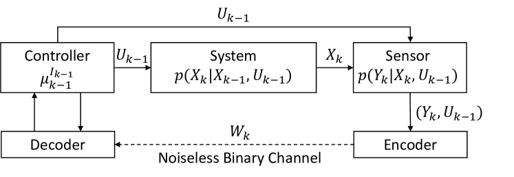
V-A Networked Control Rate-Cost Trade-Offs
Consider a networked control setting in which the feedback path of a POMDP involves transmission over a noiseless binary channel, as illustrated in Fig. 1(a). At every time step , an encoder receives observations of the state (e.g., arising from a sensor), and selects and transmits a binary codeword from a predefined codebook of optimal uniquely decodable binary codes . Upon receiving , the decoder decodes and passes it to a controller, that uses it to evaluate the next control . We allow the codebook to be time-varying, and let be the length (number of bits) of the codeword . We assume that both the encoder and decoder have infinite memories so that conveys given . Shannon’s source coding theorem (cf. [23, Section 5.5]) then implies that the (minimum) expected data transmitted in the noiseless binary channel at time satisfies
and so the total expected data transmitted over satisfies
In view of Lemma III.2 and Theorem III.1, our ERPOMDP problem (7) with (and any ) thus has the operational interpretation of seeking policies that trade-off the expected total data transmitted for feedback control via , with the value of the cost functional .
Theorem III.1 is particularly important for introducing rate-cost trade-offs into POMDPs because it enables regularization only by the input-output entropy (i.e., it holds when but in (7)). In contrast, Theorem IV.1 is, in general, of secondary value for introducing rate-cost trade-offs because it also requires regularization by the smoother entropy (i.e., it holds only when in (7)), but does enable the use of standard POMDP techniques without PWLC approximations.
V-B Memory-Efficient Active State Trajectory Estimation
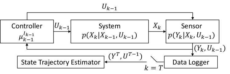
The second operational interpretation of our ERPOMDP problem (7) relates to active state estimation (i.e. controlling a POMDP to aid the estimation of its latent state trajectory from stored trajectories ). Such problems arise in robotics (cf. [13, 14]) and controlled sensing (cf. [9, 10]).
As shown in Fig. 1(b), consider a POMDP in which, at each time , the current observation and control are encoded and stored by a data logger by selecting and storing a binary codeword from a predefined codebook of optimal uniquely decodable binary codes . Thus, the data logger encodes given . We allow the codebook to be time-varying, and let be the length of the codeword . Shannon’s source coding theorem (cf. [23, Section 5.5]) implies that the (minimum) expected total memory required to store satisfies the bounds
At the conclusion of the control horizon (), the data logger decodes the stored trajectories and passes them to an (offline) algorithm for estimating the state trajectory (e.g. the Viterbi algorithm). Let the minimum probability of error for any estimator of given be with being any function . Theorem 1 of [29] gives that
where and are the inverse functions of strictly monotonically increasing functions (defined in [29]), and thus are themselves strictly monotonically increasing.
The involvement of the smoother and input-output entropies in bounds on the estimation error and required memory implies that (7) has the operational interpretation of seeking policies that aid estimation of the state trajectory (by reducing the smoother entropy) whilst decreasing the memory required to store the observation and control trajectories (by reducing the input-output entropy). In the special case considered in Section IV with , (7) constitutes a formulation of active state estimation in which the estimation and memory objectives are weighted equally. In this regard, Theorem IV.1 establishing the linearity of in (19) is further surprising since most previous active state estimation formulations involve cost that are entirely nonlinear in the belief state and can only be optimized by resorting to approximations (cf. [9, 6, 10]).
V-C Relationship to Other Information-Theoretic POMDPs
ERPOMDPs (7) are closely related to problems involving the optimization of information-theoretic terms that have previously been considered for reinforcement learning [30], studying the capacity of channels with memory and feedback [31], privacy (e.g. in smart metering systems) [32, 33, 21, 19], and studying rate-cost trade-offs in MDPs and POMDPs [2, 8]. These problems, however, mostly involve optimizing only a single information-theoretic term derived from either the mutual information between states and/or observations (e.g., directed information and transfer entropy [31, 32, 19, 2, 8, 21]), or the entropy of the states or controls (e.g., [30, 33]). In contrast, ERPOMDPs involve both the standard cost functional and, in general, two information-theoretic terms, the smoother entropy and the (novel) input-output entropy. The procedure for solving ERPOMDPs is, however, similar to that of solving these other optimization problems, with most having been shown to lead to belief MDPs — albeit few (if any) with cost functions that are linear in the belief state, rendering our Theorem IV.1 joint-entropy result further surprising.
VI Simulation Example
We now simulate ERPOMDPs for active state estimation.
VI-A Example Set-Up
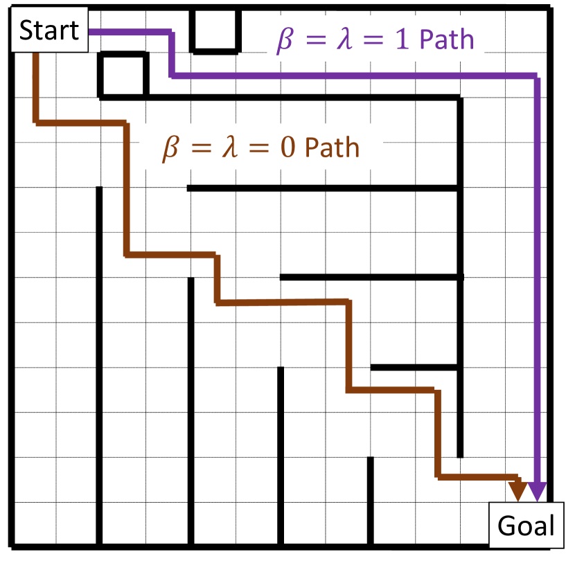
Consider an agent in the grid shown in Fig. 2, that seeks to move to (and stay in) a known goal location from an unknown starting location (distributed uniformly over the grid such that the initial state pmf is uniform), whilst actively localizing itself so as to enable its path to the goal to be estimated for the purpose of later being retraced or communicated. Each cell in the grid is a state in the agent’s state space (enumerated top-to-bottom, left-to-right). The agent has five possible control actions , corresponding to moving one cell in each of the four compass directions, or staying still (all with probability ). There are internal and external walls (bold black lines in Fig. 2) that block movement, with the agent staying still if it attempts to move into them. The agent receives measurements corresponding to whether or not a wall is immediately adjacent to its current cell in each of the four compass directions. The agent detects a wall when it is present (resp. not present) with probability (resp. ). A simplified version of this example was previously considered in [2] for MDPs.
We examine the ability of the agent to move to the goal and ensure estimation of its path by solving (7) with either (corresponding to a standard POMDP without any regularization), (corresponding to joint-entropy regularization), and (corresponding to only smoother-entropy regularization), and and (corresponding to only input-output-entropy regularization). In all cases, and the goal objective is encoded via the cost for all and .
We use SARSOP [24] to solve (7) via the reformulation in Theorem IV.1 when , and via the reformulation in Theorem III.1 when . For , we construct a PWLC approximation of in (17) using a set containing the middle of the simplex and points near the vertices with values in their largest element of and in their other elements. For , we avoid PWLC approximations since the cost function in Theorem IV.1 is linear. From Table I, we see that the time taken to compute policies requiring PWLC approximations (i.e., policies with ) is much greater than the time required to compute the standard POMDP policy with , and the ERPOMDP policy with .
VI-B Simulation Results
The results of Monte Carlo simulations of each policy over time steps (the mean of ) are summarized in Table I. For each policy, we report several active state estimation criteria including: the total (undiscounted) cost associated with not being in the goal state (i.e., the Goal Cost) ; the input-output entropy; the smoother entropy; the joint entropy; the sum of belief entropies ; and, the probability of error in maximum a posteriori estimates of the trajectory (Traj. MAP Error Prob.) computed via the Viterbi algorithm [10, Section 3.5.3]. Example state realizations with the agent starting in the top-left cell are shown in Fig. 2.
Table I shows that the standard POMDP policy () results in the lowest goal cost, which is unsurprising since it only explicitly minimizes the (discounted) cost of the agent not being in the goal state. The smoother entropy, input-output entropy, and joint entropy are all significantly less (better) when they are regularized via selection of and , and , or both , respectively (at the expense of a small increase in the Goal Cost). Table I thus highlights that the agent resolves its uncertainty and reduces the memory required to store its measurements more effectively with versions of ERPOMDP policies with nonzero and than with the standard POMDP policy (with ).
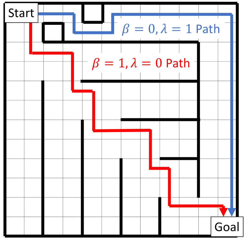
As illustrated in Fig. 2, the ERPOMDP policies with , and and , reduce the joint entropy and input-output entropy most effectively by moving the agent through the cells along the walls since these yield easily compressible observation sequences (a single wall in the same relative direction). In contrast, the cells in the center through which the standard POMDP policy (with ) and the ERPOMDP policy with and move the agent yield more variable (higher entropy) observations since they are surrounded by , , or walls. By initially moving the agent East from its starting cell and then through the center, the ERPOMDP policy with and is able to achieve the minimum smoother entropy. However, in this example, the differences in smoother entropies between policies with and is much smaller compared to the differences in input-output entropies between policies with and . Thus, the ERPOMDP policy involving joint-entropy regularization via achieves close to the best performance across the criteria (at the slight expense of the Goal Cost) whilst avoiding PWLC approximations, highlighting the value of Theorem IV.1. Clearly, finer trade-offs between the Goal Cost and smoother or input-output entropies can be obtained by selecting and independently and using Theorem III.1, but at considerable computational cost.
| Performance Criteria | ERPOMDP (7) Policy Parameters | |||
|---|---|---|---|---|
| Goal Cost | 23.0 | 25.2 | 25.9 | 26.0 |
| Input-Output Entropy | 120.2 | 122.0 | 114.9 | 114.9 |
| Smoother Entropy | 1.47 | 0.41 | 0.60 | 0.50 |
| Joint Entropy | 121.7 | 122.4 | 115.5 | 115.4 |
| Sum of Belief Entropies | 21.9 | 17.3 | 16.0 | 16.0 |
| Traj. MAP Error Prob. | 0.01 | 0.00 | 0.01 | 0.00 |
| Time to Compute Policy (s) | 0.21 | 6563 | 964 | 0.66 |
VII Conclusion
We propose ERPOMDPs, show that they admit PWLC approximate solutions, and discuss their relevance to active state estimation and rate-cost trade-offs. Surprisingly, ERPOMDPs admit exact solutions when regularizing by the joint entropy of the states, observations, and controls, which constitutes a novel, tractable formulation of active state estimation.
References
- [1] T. L. Molloy and G. N. Nair, “JEM: Joint Entropy Minimization for Active State Estimation with Linear POMDP Costs,” in 2022 American Control Conference (ACC), 2022, pp. 1601–1607.
- [2] T. Tanaka, H. Sandberg, and M. Skoglund, “Transfer-Entropy-Regularized Markov Decision Processes,” IEEE Transactions on Automatic Control, pp. 1–1, 2021.
- [3] E. Shafieepoorfard, M. Raginsky, and S. P. Meyn, “Rationally inattentive control of Markov processes,” SIAM Journal on Control and Optimization, vol. 54, no. 2, pp. 987–1016, 2016.
- [4] G. M. Hoffmann and C. J. Tomlin, “Mobile sensor network control using mutual information methods and particle filters,” IEEE Transactions on Automatic Control, vol. 55, no. 1, pp. 32–47, 2010.
- [5] T. L. Molloy and G. N. Nair, “Active trajectory estimation for partially observed Markov decision processes via conditional entropy,” in 2021 European Control Conference (ECC), 2021, pp. 385–391.
- [6] M. Araya, O. Buffet, V. Thomas, and F. Charpillet, “A POMDP extension with belief-dependent rewards,” in Advances in Neural Information Processing Systems, J. Lafferty, C. Williams, J. Shawe-Taylor, R. Zemel, and A. Culotta, Eds., vol. 23. Curran Associates, Inc., 2010, pp. 64–72.
- [7] M. Fehr, O. Buffet, V. Thomas, and J. Dibangoye, “rho-POMDPs have Lipschitz-Continuous epsilon-Optimal Value Functions,” in Advances in Neural Information Processing Systems, S. Bengio, H. Wallach, H. Larochelle, K. Grauman, N. Cesa-Bianchi, and R. Garnett, Eds., vol. 31. Curran Associates, Inc., 2018.
- [8] J. Rubin, O. Shamir, and N. Tishby, “Trading value and information in MDPs,” in Decision Making with Imperfect Decision Makers. Springer, 2012, pp. 57–74.
- [9] V. Krishnamurthy and D. V. Djonin, “Structured threshold policies for dynamic sensor scheduling – a partially observed Markov decision process approach,” IEEE Transactions on Signal Processing, vol. 55, no. 10, pp. 4938–4957, 2007.
- [10] V. Krishnamurthy, Partially observed Markov decision processes. Cambridge University Press, 2016.
- [11] D.-S. Zois and U. Mitra, “Active state tracking with sensing costs: Analysis of two-states and methods for -states,” IEEE Transactions on Signal Processing, vol. 65, no. 11, pp. 2828–2843, 2017.
- [12] D.-S. Zois, M. Levorato, and U. Mitra, “Active classification for POMDPs: A Kalman-like state estimator,” IEEE Transactions on Signal Processing, vol. 62, no. 23, pp. 6209–6224, 2014.
- [13] S. Thrun, W. Burgard, and D. Fox, Probabilistic Robotics. MIT Press, 2005.
- [14] C. Stachniss, G. Grisetti, and W. Burgard, “Information gain-based exploration using Rao-Blackwellized particle filters.” in Robotics: Science and Systems, vol. 2, 2005, pp. 65–72.
- [15] R. Valencia, J. Valls Miró, G. Dissanayake, and J. Andrade-Cetto, “Active Pose SLAM,” in 2012 IEEE/RSJ International Conference on Intelligent Robots and Systems, 2012, pp. 1885–1891.
- [16] T. L. Molloy and G. N. Nair, “Smoother Entropy for Active State Trajectory Estimation and Obfuscation in POMDPs,” arXiv preprint arXiv:2108.10227, 2021.
- [17] E. G. Ryan, C. C. Drovandi, J. M. McGree, and A. N. Pettitt, “A review of modern computational algorithms for Bayesian optimal design,” International Statistical Review, vol. 84, no. 1, pp. 128–154, 2016.
- [18] K. Chaloner and I. Verdinelli, “Bayesian experimental design: A review,” Statistical Science, pp. 273–304, 1995.
- [19] T. Tanaka, P. M. Esfahani, and S. K. Mitter, “LQG control with minimum directed information: Semidefinite programming approach,” IEEE Trans. on Automatic Control, vol. 63, no. 1, pp. 37–52, 2018.
- [20] V. Kostina and B. Hassibi, “Rate-cost tradeoffs in control,” IEEE Trans. on Automatic Control, vol. 64, no. 11, pp. 4525–4540, 2019.
- [21] O. Sabag, P. Tian, V. Kostina, and B. Hassibi, “The Minimal Directed Information Needed to Improve the LQG Cost,” in 2020 59th IEEE Conference on Decision and Control (CDC), 2020, pp. 1842–1847.
- [22] A. Shwartz, “Death and discounting,” IEEE Transactions on Automatic Control, vol. 46, no. 4, pp. 644–647, 2001.
- [23] T. Cover and J. Thomas, Elements of information theory, 2nd ed. New York: Wiley, 2006.
- [24] H. Kurniawati, D. Hsu, and W. S. Lee, “SARSOP: Efficient point-based POMDP planning by approximating optimally reachable belief spaces.” in Robotics: Science and Systems, 2008.
- [25] N. P. Garg, D. Hsu, and W. S. Lee, “DESPOT-Alpha: Online POMDP planning with large state and observation spaces.” in Robotics: Science and Systems, 2019.
- [26] G. Kramer, “Directed information for channels with feedback,” Ph.D. dissertation, Swiss Federal Institute of Technology, Zurich, 1998.
- [27] D. P. Bertsekas, Dynamic programming and optimal control, Third ed. Belmont, MA: Athena Scientific, 1995, vol. 1.
- [28] R. Fiorenza, Hölder and locally Hölder Continuous Functions, and Open Sets of Class , . Birkhäuser, 2017.
- [29] M. Feder and N. Merhav, “Relations between entropy and error probability,” IEEE Trans. on Info. Theory, vol. 40, no. 1, pp. 259–266, 1994.
- [30] T. Haarnoja, H. Tang, P. Abbeel, and S. Levine, “Reinforcement learning with deep energy-based policies,” in International Conference on Machine Learning. PMLR, 2017, pp. 1352–1361.
- [31] C. D. Charalambous and P. A. Stavrou, “Directed information on abstract spaces: Properties and variational equalities,” IEEE Transactions on Information Theory, vol. 62, no. 11, pp. 6019–6052, 2016.
- [32] S. Li, A. Khisti, and A. Mahajan, “Information-theoretic privacy for smart metering systems with a rechargeable battery,” IEEE Trans. on Information Theory, vol. 64, no. 5, pp. 3679–3695, 2018.
- [33] Y. Savas, M. Ornik, M. Cubuktepe, M. O. Karabag, and U. Topcu, “Entropy maximization for Markov decision processes under temporal logic constraints,” IEEE Trans. on Automatic Control, vol. 65, no. 4, pp. 1552–1567, 2020.