A family of consistent normally distributed tests for Poissonity

Abstract

A consistent test based on the probability generating function is proposed for assessing Poissonity against a wide class of count distributions, which includes some of the most frequently adopted alternatives to the Poisson distribution. The statistic, in addition to have an intuitive and simple form, is asymptotically normally distributed, allowing a straightforward implementation of the test. The finite sample properties of the test are investigated by means of an extensive simulation study. The test shows a satisfactory behaviour compared to other tests with known limit distribution.

1 Introduction

Assessing the Poissonity assumption is a relevant issue of statistical inference, both because Poisson distribution has an impressive list of applications in biology, epidemiology, physics and queue theory (see e.g. Johnson et al.,, 2005; Puig and Weiß,, 2020) and because it is a preliminary step in order to apply many popular statistical models. The use of the probability generating function (p.g.f.) has a long tradition (see e.g. Kocherlakota and Kocherlakota,, 1986; Meintanis and Bassiakos,, 2005; Rémillard and Theodorescu,, 2000) for testing discrete distributions and some omnibus procedures based on the p.g.f. have been proposed for Poissonity (e.g. Nakamura and Pérez-Abreu,, 1993; Baringhaus and Henze,, 1992; Rueda and O’Reilly,, 1999; Gürtler and Henze,, 2000; Meintanis and Nikitin,, 2008; Inglot,, 2019; Puig and Weiß,, 2020). Omnibus tests are particularly appealing since they are consistent against all possible alternative distributions but they commonly have a non-trivial asymptotic behavior. Moreover, the distribution of the test statistic may depend on the unknown value of the Poisson parameter, implying the necessity to use computationally intensive bootstrap, jackknife or other resampling methods to approximate it. On the other hand, Poissonity tests against specific alternatives may achieve high power but rely on the knowledge of what deviations from Poissonity can occurr. An alternative approach, proposed by Meintanis and Nikitin, (2008), is to consider tests with suitable asymptotic properties with respect to a fairly wide class of alternatives, which are also the most likely when dealing with the Poissonity assumption.

In this paper, by referring to the same class of alternative distributions and by using the characterization of the Poisson distribution based on its p.g.f., we propose a family of consistent and asymptotically normally distributed test statistics and a data-driven procedure for the choice of the parameter indexing the statistics. In particular, the test statistics not only have an intuitive interpretation, but, being extremely simple to compute, allow a straightforward implementation of the test and lead to test procedures with satisfactory performance also in presence of contiguous alternatives.

2 Characterization of the Poisson distribution

Let $X$ be a random variable (r.v.) taking natural values with probability mass function $p_{X}$ and ${\rm E}[X]=\mu$. Moreover, let $\Psi_{X}(t)={\rm E}[t^{X}]$, with $t\in[0,1]$, be the p.g.f. of $X$. Following Meintanis and Nikitin, (2008), we consider the class of count distributions $\Delta$ such that

$$D(t,\mu)=\Psi_{X}^{\prime}(t)-\mu\Psi_{X}(t)$$

is not negative for any $t\in[0,1]$ or not positive for any $t\in[0,1]$ for all $\mu>0$, where $\Psi_{X}^{\prime}(t)$ is the first order derivative of the p.g.f..

This class contains many popular alternatives to the Poisson distribution, such as the Binomial distribution, the Negative Binomial distribution, the generalized Hermite distribution, the Zero-Inflated mixtures.

It must be pointed out that $D(t,\mu)=0$ for any $t\in[0,1]$ and for some $\mu>0$ if and only if $X$ is a Poisson r.v.. This characterization allows to construct a goodness of fit test for Poissonity against alternatives belonging to the class $\Delta$, that is for the hypothesis system

$$H_{0} :X\in\Pi_{\mu},\text{for some}\ \mu>0$$

$$H_{1} :X\in\Delta$$

where $\Pi_{\mu}$ denotes the Poisson distribution with parameter $\mu$. In particular, Meintanis and Nikitin, (2008) adopt the previous characterization to construct a consistent test for the Poisson distribution by means of the empirical counterpart of $D(t,\mu)$ suitably weighted. An alternative approach can be based on the $L^{1}$ distance of $D(t,\mu)$ from $0$, whose positive values evidence departures from Poissonity. The following Proposition, giving bounds for this distance, provides insight into the introduction of a family of test statistics.

Proposition 1.

For any natural number $k$, let $f_{k}(\mu)=e^{-\mu}(1+\ldots+{\frac{\mu^{k}}{k!}}).$ For any $X\in\Delta$ and for any $\mu>0$, it holds

$$\frac{1}{1+\ldots+{\frac{\mu^{k}}{k!}}}|T^{(k)}|\leq\int_{0}^{1}|D(t,\mu)|\,dt\leq {e^{\mu}}|T^{(k)}|,$$ (1)

where $T^{(k)}=f_{k}(\mu)-p_{X}(0)(1+\ldots+{\frac{\mu^{k}}{k!}}).$ In particular, for $k=0$,

$$|e^{-\mu}-p_{X}(0)|\leq\int_{0}^{1}|D(t,\mu)|\,dt\leq e^{\mu}\,|e^{-\mu}-p_{X}(0)|.$$

Proof.

Since $X\in\Delta$

$$\big{|}\int_{0}^{1}D(t,\mu)e^{-\mu t}\,dt\big{|} \leq\int_{0}^{1}|D(t,\mu)|\,dt=\int_{0}^{1}e^{\mu t}|D(t,\mu)e^{-\mu t}|\,dt$$

$$\leq e^{\mu}\int_{0}^{1}|D(t,\mu)e^{-\mu t}|\,dt=e^{\mu}\big{|}\int_{0}^{1}D(t,\mu)e^{-\mu t}\,dt\big{|}.$$

As $D(t,\mu)e^{-\mu t}=\{\Psi_{X}(t)e^{-\mu t}\}^{\prime}$, then

$$\int_{0}^{1}D(t,\mu)e^{-\mu t}\,dt=e^{-\mu}-p_{X}(0).$$

By dividing and multiplying for $1+\ldots+{\frac{\mu^{k}}{k!}}$, the thesis immediately follows. ∎

Thanks to inequality (1), a family of test statistics, indexed by $k$ and depending on an estimator of

$$T^{(k)}=f_{k}(\mu)-p_{X}(0)\Big{(}1+\ldots+{{\mu^{k}}\over{k!}}\Big{)}$$

can be defined. Note that $f_{k}(\mu)$ and $p_{X}(0)(1+\ldots+{\frac{\mu^{k}}{k!}})$ are equal to $P(X\leq k)$ when $X$ belongs to $\Pi_{\mu}$ and obviously $T^{(k)}\neq 0$ for some $k\geq 0$ iff $X$ is not a Poisson r.v. iff $T^{(0)}\neq 0$. Thus, the simplest test statistic arises from an estimator of $T^{(0)}=e^{-\mu}-p_{X}(0)$. The corresponding test statistic is really appealing owing to its simplicity and its straightforward interpretation, comparing the probability that $X$ takes value zero with the probability of zero for a Poisson r.v., but its performance may deteriorate with respect to those based on $T^{(k)}$ for $k>0$, especially when the sample size is small while $\mu$ is relatively large, as the estimation of $p_{X}(0)$ becomes even more crucial.

3 The test statistic

Given a random sample $X_{1},\ldots,X_{n}$ from $X$, let $\overline{X}_{n}$ and $F_{n}$ be the mean and the empirical cumulative distribution function, that is

$$\overline{X}_{n}=\frac{X_{1}+\ldots+X_{n}}{n},\ \ F_{n}(k)=\frac{I{(X_{1}\leq k)}+\ldots+I{(X_{n}\leq k)}}{n}.$$

It is at once apparent that $T^{(k)}$ can be estimated by means of

$$\widehat{T}_{n}^{(k)}=f_{k}(\overline{X}_{n})-F_{n}(k).$$

Since $k$ is a fixed natural number (often $k=0$), $\widehat{T}_{n}^{(k)}$ is not a random process but simply a r.v. whose asymptotic distribution can be easily derived from classical Central Limit Theorems, as shown in the following Proposition.

Proposition 2.

Let $X$ be a r.v. with ${\rm Var}[X]$ finite and $k$ be a fixed natural number. Let

$$V^{(k)}_{n}=\sqrt{n}\,\widehat{T}_{n}^{(k)}.$$

If $X\in\Pi_{\mu}$ then $V_{n}^{(k)}$ converges in distribution to ${\mathcal{N}}(0,\sigma^{2}_{\mu,k})$ as $n\to\infty$, where

$$\sigma^{2}_{\mu,k}={\rm Var}\Big{[}e^{-\mu}{\frac{\mu^{k}}{k!}}X+I(X\leq k)\Big{]}=f_{k}(\mu)\{1-f_{k}(\mu)\}-{\frac{e^{-2\mu}\mu^{2k+1}}{(k!)^{2}}}.$$ (2)

Moreover, if $r_{k}=P(X\leq k)-f_{k}(\mu)\neq 0$ for some $k,$ namely $X$ is not a Poisson r.v., then $|V_{n}^{(k)}|$ converges in probability to $\infty$.

Proof.

Note that $f^{\prime}_{k}(\mu)=-e^{-\mu}\frac{\mu^{k}}{k!}.$ Owing to the Delta Method

$$V_{n}^{(k)} =\sqrt{n}\{f_{k}(\overline{X}_{n})-f_{k}(\mu)+f_{k}(\mu)-F_{n}(k)\}$$

$$=-\sqrt{n}\{e^{-\mu}{\frac{\mu^{k}}{k!}}(\overline{X}_{n}-\mu)+F_{n}(k)-f_{k}(\mu)\}+o_{P}(1)$$

$$={\frac{g(X_{1})+\ldots+g(X_{n})}{\sqrt{n}}}-\sqrt{n}r_{k}+o_{P}(1),$$

where $g$ is the function defined by $x\mapsto-e^{-\mu}{\frac{\mu^{k}}{k!}}(x-\mu)-\{I(x\leq k)-P(X\leq k)\}$. When $X\in\Pi_{\mu}$, $r_{k}=0$, ${\rm E}[g(X)]=0$ and ${\rm E}[o_{P}^{2}(1)]$ is $o(1)$ since $|f_{k}(\overline{X}_{n})-f_{k}(\mu)|\leq|\overline{X}_{n}-\mu|.$ Then, under $H_{0}$, $V_{n}^{(k)}$ is proven to converge in distribution to ${\mathcal{N}}(0,{{\rm Var}\,[g(X)]})$ by applying the Central Limit Theorem to ${\frac{g(X_{1})+\ldots+g(X_{n})}{\sqrt{n}}}$. Moreover, since

$${\rm Var}\,[g(X)]={\frac{e^{-2\mu}\mu^{2k+1}}{(k!)^{2}}}+f_{k}(\mu)\{1-f_{k}(\mu)\}+2e^{-\mu}{\frac{\mu^{k}}{k!}}{\rm Cov}\,\big{[}X,I(X\leq k)\big{]}$$

and

$${\rm Cov}\,\big{[}X,I(X\leq k)\big{]}=\sum_{j=1}^{k}\frac{e^{-\mu}\mu^{j}}{(j-1)!}-\mu f_{k}(\mu)=-e^{-\mu}{\frac{\mu^{k+1}}{k!}},$$

the first part of the proposition is proven.

Now, let $X$ be a r.v. such that $r_{k}\neq 0$, in particular $X$ is not a Poisson r.v.. Thus, $|V_{n}^{(k)}|$ converges in probability to $\infty$ because ${\frac{g(X_{1})+\ldots+g(X_{n})}{\sqrt{n}}}+o_{P}(1)$ is bounded in probability and $\sqrt{n}|r_{k}|$ converges to $\infty$. The second part of the proposition is so proven.

∎

Thanks to Proposition 2, fixed a natural number $k\geq 0$ and under the null hypothesis $H_{0}$, $\sqrt{n}\,\widehat{T}_{n}^{(k)}/\sigma_{\mu,k}$ converges to ${\mathcal{N}}(0,1)$. Therefore, an estimator of $\sigma_{\mu,k}$ is needed to define the test statistic. As the plug-in estimator

$$\widetilde{\sigma}^{2}_{n,k}=e^{-2\overline{X}_{n}}\big{\{}\big{(}1+\ldots+{{\overline{X}_{n}^{k}}\over{k!}}\big{)}\big{(}e^{\overline{X}_{n}}-1-\ldots-{{\overline{X}_{n}^{k}}\over{k!}}\big{)}-{{\overline{X}_{n}^{2k+1}}\over{(k!)^{2}}}\big{\}}$$

converges a.s. and in quadratic mean to $\sigma^{2}_{\mu,k}$, for any natural number $k$, the test statistic turns out to be

$$Z_{n,k}=\frac{\sqrt{n}\,\widehat{T}_{n}^{(k)}}{\widetilde{\sigma}_{n,k}}.$$

An $\alpha$-level large sample test rejects $H_{0}$ for realizations of the the test statistic whose absolute values are greater than $z_{1-\alpha/2}$, where $z_{1-\alpha/2}$ denotes the ${1-\alpha/2}$-quantile of the standard normal distribution.

Corollary 1.

Under $H_{1}$, for any natural number $k$ such that $P(X\leq k)-f_{k}(\mu)\neq 0$, $Z_{n,k}$ converges in probability to $\infty$.

Proof.

As $\widetilde{\sigma}^{2}_{n,k}$ converges a.s. to $\sigma^{2}_{\mu,k}$, the proof immediately follows from the second part of Proposition 2. ∎

It is at once apparent that $Z_{n,k}$ actually constitutes a family of test statistics giving rise to consistent test for $k=0$ and for all the other values of $k$ for which there is a discrepancy between the cumulative distribution of the Poisson and of $X$. The statistic $Z_{n,0}$ is really appealing owing to its simplicity and its straightforward interpretation, comparing estimators of the probability that $X$ takes value zero and of the probability of zero for a Poisson r.v., but its finite-sample performance may deteriorate, especially when the sample size is small while $\mu$ is relatively large. Therefore, the selection of the parameter $k$ ensuring consistency and good discriminatory capability is crucial and a data-driven selection criterion is proposed.

4 Data-driven choice of $k$

An euristic, relatively simple, criterion for choosing $k$ is based on the relative discrepancy measure $T_{n}^{(k)}/f_{k}(\mu)$ which can be estimated by $\frac{\widetilde{\sigma}_{n,k}}{f_{k}(\overline{X}_{n})\sqrt{n}}Z_{n,k}$. Recalling that, under $H_{0}$, $Z_{n,k}$ is approximately a standard normal r.v. also for moderate sample size, as $\frac{\widetilde{\sigma}_{n,k}}{f_{k}(\overline{X}_{n})\sqrt{n}}$ converges a.s. to $0$ when $n\to\infty$, for any fixed $n$, $k$ may be selected in a such a way that $\frac{\widetilde{\sigma}_{n,k}}{f_{k}(\overline{X}_{n})\sqrt{n}}$ is not negligible. This choice should ensure both high power and an actual significance level close to the nominal one. To this purpose, note that the function $\mu\mapsto f_{k}(\mu)$ is decreasing for any $k$ and if $\mu\geq 1$, it holds $f^{2}_{k}(\mu)/f_{k}(1)\leq f_{k}(\mu)$ and $\sup_{k}1/f_{k}(\mu)=1/f_{0}(1)=e$. Then $k$ can be selected as the smallest natural number such that $\frac{\widetilde{\sigma}_{n,k}}{f^{2}_{k}(\overline{X}_{n})\sqrt{n}}$ is not greater than $e$ when $\overline{X}_{n}\geq 1$, that is

$$k^{*}_{n}=\min\Big{\{}k\geq 0:I(\overline{X}_{n}\geq 1)\,\frac{\widetilde{\sigma}_{n,k}}{f^{2}_{k}(\overline{X}_{n})\sqrt{n}}\leq e\Big{\}}.$$

Notwithstanding $k^{*}_{n}$ converges a.s. to $0$ since ${\widetilde{\sigma}_{n,k}}\leq 1/2$ from (2), the convergence rate may be very slow for large values of $\mu$ in such a way that $k^{*}_{n}$ can be rather larger than $0$ even for large sample sizes. Finally, by considering the test statistic corresponding to $k^{*}_{n}$

$$W_{n}=\frac{\sqrt{n}\,\widehat{T}_{n}^{(k^{*}_{n})}}{\widetilde{\sigma}_{n,k^{*}_{n}}},$$

its asymptotic behaviour can be obtained.

Corollary 2.

Under $H_{0}$, $W_{n}$ converges in distribution to ${\mathcal{N}}(0,1)$ as $n\to\infty$ and, under $H_{1}$, $W_{n}$ converges in probability to $\infty$.

Proof.

Since $k^{*}_{n}$ converges to 0, $W_{n}$ and $Z_{n,0}$ have the same asymptotic behaviour and the proof immediately follows from Proposition 2 and Corollary 1. ∎

It is worth noting that the selection of $k_{n}^{*}$ by means of the proposed data-driven criterion ensures consistency, maintaining the asymptotic normal distribution of the test statistic.

5 Asymptotic behaviour under contiguous alternatives

The asymptotic behaviour of the proposed test is investigated for detecting Poisson departures from contiguous alternative mixtures of distributions, which can be hardly recognized. More precisely, given a positive number $\lambda$, for any $n\geq\lambda^{2}$, let

$$X^{(n)}\sim I(A_{n})X+I(A^{c}_{n})Y$$ (3)

where $X\in\Pi_{\mu}$, $Y$ is a positive random variable with ${\rm E}[Y]=\mu$ and ${\rm E}[Y^{2}]<\infty$, $X,Y,I(A_{n})$ are independent and $P(A_{n})=(1-\frac{\lambda}{\sqrt{n}})$. Note that $X^{(n)}$ belongs to $\Delta$ if $Y$ belongs to $\Delta$ and converges to a Poisson r.v..

Proposition 3.

For any $n\geq\lambda^{2}$, given a random sample $X^{(n)}_{1},\ldots,X^{(n)}_{n}$ from $X^{(n)}$, for a fixed natural number $k$, let

$$U^{(k)}_{n}=\sqrt{n}\,\big{\{}f_{k}\big{(}\overline{X}_{n}^{\prime}\big{)}-F^{\prime}_{n}(k)\big{\}}$$

where $\overline{X}_{n}^{\prime}$ and $F^{\prime}_{n}$ are the sample mean and the empirical cumulative distribution function. Then $U_{n}^{(k)}$ converges in distribution to ${\mathcal{N}}(\tau_{k},\sigma^{2}_{\mu,k})$ as $n\to\infty$, where $\tau_{k}=-\lambda\{P(Y\leq k)-f_{k}(\mu)\}$. In particular $U^{(k^{*}_{n})}_{n}$, where $k^{*}_{n}$ is obtained by the data-driven criterion, is equivalent to $U^{(0)}_{n}$, which converges in distribution to ${\mathcal{N}}(\lambda\{e^{-\mu}-P(Y=0)\},e^{-2\mu}(e^{\mu}-1-\mu))$.

Proof.

Note that $|f^{\prime\prime}_{k}|\leq 2$ for any $k$. Owing to the Taylor’s Theorem

$$|\sqrt{n}\,\{f_{k}\big{(}\overline{X}_{n}^{\prime}\big{)}-f_{k}(\mu)\}+\sqrt{n}e^{-\mu}{\frac{\mu^{k}}{k!}}\big{(}\overline{X}_{n}^{\prime}-\mu)|\leq\sqrt{n}(\overline{X}_{n}^{\prime}-\mu)^{2}$$

Since

$${\rm E}\big{[}\sqrt{n}(\overline{X}_{n}^{\prime}-\mu)^{2}\big{]}\leq\frac{\mu+{\rm Var}[Y]}{\sqrt{n}},$$

$U^{(k)}_{n}$ and ${\frac{g_{n}(X^{(n)}_{1})+\ldots+g_{n}(X^{(n)}_{n})}{\sqrt{n}}}-\sqrt{n}r_{n,k}$ have the same asymptotic behaviour, where $g_{n}$ is the function defined by $x\mapsto-e^{-\mu}{\frac{\mu^{k}}{k!}}(x-\mu)-\{I(x\leq k)-P(X^{(n)}\leq k)\}$ and $r_{n,k}=P(X^{(n)}\leq k)-f_{k}(\mu)$. Since $\lim_{n}-\sqrt{n}r_{n,k}=\lambda^{*}_{k}$, the thesis follows from the convergence in distribution of ${\frac{g_{n}(X^{(n)}_{1})+\ldots+g_{n}(X^{(n)}_{n})}{\sqrt{n}}}$ to ${\mathcal{N}}(0,\sigma^{2}_{\mu,k}).$ ∎

The previous proposition can be considered a non-parametric version of classical asymptotic analysis under so-called shrinking alternative. Moreover the test statistic has a local asymptotic normal distribution which is useful to highlight its discriminatory capability under not trivial contiguous alternatives. In a parametric setting, by means of Le Cam lemmas (Le Cam,, 2012), it could be possible to derive the limiting power function and to build an efficiency measure for test statistics. Clearly in a non-parametric functional setting, a closed form of the power function is not available and must be assessed by means of simulations studies.

6 Simulation study

The performance of the proposed test has been assessed by means of an extensive Monte Carlo simulation. First of all, fixed the nominal level $\alpha=0.05$, the significance level of the test is empirically evaluated, as the proportion of rejections of the null hypothesis, by independently generating $10000$ samples of size $n=50$ from Poisson distributions with $\mu$ varying from $0.5$ to $16$ by $0.2$. As early mentioned, the family of test statistics $Z_{n,k}$ depends on the parameter $k$ and therefore, for any $\mu$, the empirical significance level is computed for $k=0,1,2,3$ and reported in Figure 1. Simulation results confirm that for large values of $\mu$ the empirical level is far from the nominal one even for reasonably large sample size and that a data-driven procedure is needed to select $k$. Thus, the test statistic $W_{n}$ is considered and its performance is compared to those of two tests having known asymptotic distributions: the test by Meintanis and Nikitin, (2008), $MN_{n}$, also recommended by Mijburgh and Visagie, (2020) to achieve good power against a large variety of deviations from the Poisson distribution, and the Fisher index of dispersion, $ID_{n}$, which, owing to its simplicity, is often considered as a benchmark. The explicit ready-to-implement test statistic $MN_{n}$ has a non-trivial expression and it is based on $\int_{0}^{1}D(t,\mu)t^{a}dt,$ where $a$ is a suitable parameter. $MN_{n}$ is proven to have an asymptotic normal distribution. In the simulation $a$ is set equal to $3$ as suggested when there is no prior information on the alternative model. The Fisher index of dispersion test is performed as an asymptotic two-sided chi-square test and it is based on the extremely simple test statistic $ID_{n}={\sum_{i=1}^{n}(X_{i}-\overline{X}_{n})^{2}}/{\overline{X}_{n}}.$

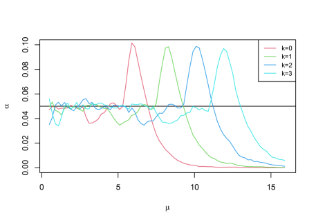
Figure 1: Empirical significance level for $k=0,1,2,3$ with $n=50$.

Initially, given $\alpha=0.05$, the three tests are compared by means of their empirical significance level computed generating $10000$ samples of size $n=20,50$ from Poisson distributions with $\mu$ varying from $0.5$ to $16$ by $0.2$. From Figure 2, it is worth noting that, even for the moderate sample size $n=20$, the test based on $W_{n}$ captures the nominal significance level satisfactory for values of $\mu$ smaller than 10, highlighting a rather good speed of convergence to the normal distribution, also confirmed by the empirical level for $n=50.$ The Fisher test shows an empirical significance level very near to the nominal one even for $n=20$, except when $\mu$ is small. The test based on $MN_{n}$, on the contrary, maintains the nominal level of significance rather closely only for $n=50$.

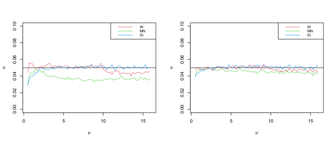
Figure 2: Empirical significance level with $n=20$ on the left and $n=50$ on the right.

The null hypothesis of Poissonity is tested against the following alternative models (for details see Johnson et al.,, 2005): mixture of two Poisson denoted by $\mathcal{MP}(\mu_{1},\mu_{2})$, Binomial by $\mathcal{B}(k,p)$, Negative Binomial by $\mathcal{NB}(k,p)$, Generalized Hermite by $\mathcal{GH}(a,b,k)$, Discrete Uniform in $\{0,1,\dots,\nu\}$ by $\mathcal{DU}(\nu)$, Discrete Weibull by $\mathcal{DW}(q,\beta)$, Logarithmic Series translated by -1 by $\mathcal{LS^{-}}(\theta)$, Logarithmic Series by $\mathcal{LS}(\theta)$, Generalized Poisson denoted by $\mathcal{GP}(\mu_{1},\mu_{2})$, Zero-inflated Binomial denoted by $\mathcal{ZB}(k,p_{1},p_{2})$, Zero-inflated Negative Binomial by $\mathcal{ZNB}(k,p_{1},p_{2})$, Zero-inflated Poisson by $\mathcal{ZP}(\mu_{1},\mu_{2})$. Various parameters values are considered (see Table 1). Moreover, the significance level of the tests are reported for Poisson distributions with $\mu=0.5,1,2,5,10,15$. The alternatives considered in the simulation study include overdispersed and underdispersed, heavy tails, mixtures and zero-inflated distributions together with distributions having mean close to variance. Some alternatives do not belong to the class $\Delta$, such as the logarithmic and shifted-logarithmic with parameters 0.7, 0.8 and 0.9 and have been included to check the robustness of the $W_{n}$ and $MN_{n}$ tests.

From each distribution, $10000$ samples of size $n=20,30,50$ are independently generated and, on each sample, the three tests are performed. The empirical power of each test is computed as the percentage of rejections of the null hypothesis. The simulation is implemented by using R Core Team, (2021) and in particular the packages extraDistr, hermite and RNGforGPD.

Simulations results are reported in Table 1. The $MN_{n}$ test is somewhat too conservative for smaller sample sizes and the $ID_{n}$ test does not capture the significance level for small $\mu$, while $W_{n}$ shows an empirical significance level rather close to the nominal one even for small sample size and small $\mu$.

As expected, also from the theoretical results by Janssen, (2000), none of the three tests shows performance superior to the others for any alternative and for any sample size and their power crucially depend on the set of parameters also for alternatives in the same class. Obviously, when the alternative model is very similar to a Poisson r.v., e.g. when the alternative is Binomial with $k$ large and $p$ small, or when dealing with the Poisson Mixtures or the Negative Binomial with $k$ large, the power of all the tests predictably decreases. Low power is also observed against slighthly overdispersed or underdispersed discrete uniform distributions, while the power rapidly increases as overdispersion becomes more marked, with the performance of all the three tests becoming comparable as $n$ increases. For the Weibull distributions the $W_{n}$ test has a certain edge over its competitors, which, on the other hand perform better when the generalized Poisson distributions are considered, even though their power is satisfactory only for ${\mathcal{G}P}(5,0.4)$. The power of the test based on $W_{n}$ is the highest for all the logarithmic distributions, with less remarkable differences for $\theta=0.9$, while the three tests exhibit nearly the same power for the shifted log-normal distribution, where a decrease in the power of $W_{n}$ occurs especially for $n=20$. As to the zero-inflated distributions, the three tests have a really unsatisfactory behaviour for $\mathcal{ZNB}(5,0.9,0.1)$ and $\mathcal{ZP}(1,0.2)$ also for $n=50$, but $W_{n}$ shows the best performance for most of the remaining alternatives and sample sizes. Overall, the number of alternatives for which the three tests reach a power greater than 90% is almost the same for $n=20$ and $n=30$. Interestingly, for $n=50$ the proposed test reaches a power greater than 90% more frequently not only than the straightforward Fisher test but also than the Meintanis test, which is more complex to be implemented.

Finally, the discriminatory capability of the tests under contiguous alternatives is evaluated. In particular, the tests based on $Z_{n,0}$, which is the simplest version of the proposed test, $MN_{n}$ and $ID_{n}$ are considered and, for sake of brevity, let $P_{n}$ be the power function corresponding to each test statistic. Obviously $P_{n}$ is a function of $\lambda$, where $\lambda\in\,\,]0,\sqrt{n}[$, which ensures that the contiguous mixture never completely degenerates, keeping its mixture nature for any $\lambda$. Hence a basic efficiency measure is the following

$$r_{n}=\frac{1}{\sqrt{n}}\int_{0}^{\sqrt{n}}P_{n}(\lambda)d\lambda$$

which evidently $r_{n}\in]0,1[$ and since $P_{n}$ is not known, the Monte Carlo estimate

$${\hat{r}}_{n}=\frac{1}{m}\sum_{i=1}^{m}\hat{P_{n}}(\lambda_{i})$$

is considered, where $\lambda_{1}=\varepsilon$, $\lambda_{i+1}=\lambda_{i}+\varepsilon$ and $\lambda_{m}=\lambda_{m-1}+\varepsilon=\sqrt{n}-\varepsilon$, for $\varepsilon$ sufficiently small, and $\hat{P_{n}}$ is the empirical power.

To assess the performance of the three tests fairly, the alternative distributions of type (3) are obtained selecting $Y$ such that the tests achieve similar power when $Y$ is the alternative distribution. In particular, $Y$ is $\mathcal{B}(1,0.5)$ and $X$ is $\Pi_{0.5}$. In Figure 3 the empirical power as a function of $\lambda$, computed on 10000 indipendently generated samples, is reported for both $n=20$ and $n=50$ sample sizes and for $\varepsilon=0.05$ and in Table 2 the corresponding values of ${\hat{r}}_{n}$ are reported.

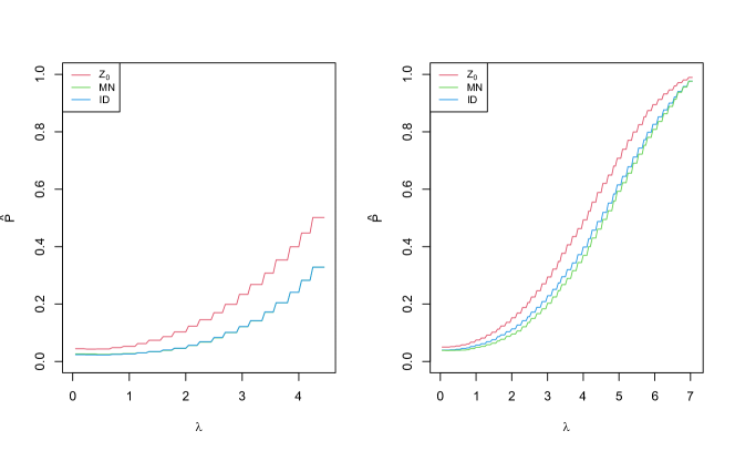
Figure 3: Empirical power against shrinking alternative with $n=20$ on the left and $n=50$ on the right.

Graphical and numerical results show that, even if all the tests improve as $n$ increases, the proposed test performs better for both sample size. The $ID_{n}$ and $MN_{n}$ tests have a similar behaviour but $ID_{n}$ seems to improve power as $n$ increases at slightly higher rate.

7 Discussion

Notwithstanding many tests for Poissonity are in literature, the proposed family of test statistics seems to be an appealing alternative in terms of simplicity, computational effort, interpretability and performance, offering better global protection against a range of alternatives in the absence of prior information regarding the type of deviation from Poissonity. Indeed, the test is consistent against any fixed alternative when $k$ is equal to $0$ and when it is selected using the data-driven criterion, that is $k=k^{*}$. For $k=0$ the test statistic basically compares an estimator of $P(X=0)$ assuming that $X$ is Poisson with the relative frequency of $0$ but the finite sample performance of the test may not be satisfactory, especially for small sample size and relatively large Poisson parameter. The performance improves for $k^{*}$, when the test juxtaposes the plug-in estimator of the cumulative distribution function of a Poisson r.v. and the empirical cumulative distribution function in $k^{*}$. Finally, even if $k^{*}_{n}$ converges a.s. to $0$, the convergence rate may be very slow for large values of the Poisson parameter, and thus, even for large sample sizes, $k^{*}_{n}$ can be rather larger than $0$.

Table 1: Empirical power with $5\%$ nominal significance level.

Model	$W_{20}$	$MN_{20}$	$ID_{20}$	$W_{30}$	$MN_{30}$	$ID_{30}$	$W_{50}$	$MN_{50}$	$ID_{50}$
$\Pi_{0.5}$	4.4	2.9	2.8	3.9	3.2	3.5	4.7	4.0	3.9
$\Pi_{1}$	5.5	4.5	4.2	4.6	4.2	4.2	4.6	4.8	4.5
$\Pi_{2}$	5.3	4.8	4.8	5.5	4.7	4.8	4.8	4.8	5.0
$\Pi_{5}$	5.4	3.7	5.2	5.6	4.3	4.8	5.2	4.6	5.0
$\Pi_{10}$	4.5	3.7	5.1	5.0	4.0	5.0	4.6	4.4	5.0
$\Pi_{15}$	4.3	3.6	5.1	4.7	4.0	4.8	4.9	4.3	5.1
$\mathcal{B}(30,0.1)$	5.9	3.7	4.8	5.8	4.5	5.4	6.4	5.7	6.7
$\mathcal{NB}(1,0.5)$	41.2	50.1	50.1	55.2	65.6	65.8	76.8	84.4	83.9
$\mathcal{NB}(4,0.75)$	11.2	15.2	16.6	14.1	20.5	22.2	21.1	29.6	32.2
$\mathcal{NB}(10,0.9)$	5.9	6.3	6.6	5.6	7.1	7.6	6.5	8.4	9.1
$\mathcal{GH}(1,1.25,2)$	18.6	50.2	43.5	27.0	65.2	58.4	43.7	84.1	78.8
$\mathcal{GH}(1,1.5,2)$	21.6	53.1	46.8	32.1	68.4	61.5	51.4	86.4	81.4
$\mathcal{GH}(1,1.75,2)$	22.3	54.9	48.5	35.1	70.1	64.0	58.9	87.8	83.8
$\mathcal{DU}(3)$	5.9	1.9	2.7	4.6	2.2	3.7	6.2	2.2	6.3
$\mathcal{DU}(5)$	6.8	18.7	4.9	9.4	26.8	6.2	15.6	41.9	8.9
$\mathcal{DU}(10)$	35.5	87.9	71.7	54.9	96.1	86.9	83.2	99.7	97.3
$\mathcal{DU}(15)$	56.6	98.1	95.3	78.9	99.8	99.1	97.4	100.0	100.0
$\mathcal{DW}(0.5,3)$	56.0	38.9	24.3	77.3	65.4	65.4	97.6	95.8	94.3
$\mathcal{DW}(0.8,5)$	100.0	99.7	99.0	100.0	100.0	100.0	100.0	100.0	100.0
$\mathcal{LS^{-}}(0.6)$	45.0	50.4	51.1	59.9	66.2	66.7	79.1	83.8	83.7
$\mathcal{LS^{-}}(0.7)$	63.3	70.0	70.1	79.0	84.9	85.0	93.9	96.3	96.0
$\mathcal{LS^{-}}(0.8)$	81.8	88.3	88.3	93.8	96.6	96.5	99.4	99.8	99.7
$\mathcal{LS^{-}}(0.9)$	94.9	98.7	98.6	99.2	99.9	99.9	100.0	100.0	100.0
$\mathcal{LS}(0.6)$	92.0	48.2	37.0	98.4	58.4	39.9	100.0	71.8	42.9
$\mathcal{LS}(0.7)$	79.8	25.4	32.1	92.0	27.1	36.0	99.1	29.8	42.5
$\mathcal{LS}(0.8)$	76.5	35.3	56.0	88.9	41.1	68.7	97.9	51.8	82.9
$\mathcal{LS}(0.9)$	91.7	83.2	91.5	97.8	92.9	97.4	99.9	98.9	99.8
$\mathcal{GP}(1,0.1)$	8.6	11.1	11.6	9.4	13.4	14.6	13.6	18.9	20.7
$\mathcal{GP}(3,0.25)$	21.9	42.8	45.6	31.7	56.7	59.6	48.2	75.8	79.3
$\mathcal{GP}(5,0.4)$	51.8	83.8	85.5	69.6	94.2	95.3	90.6	99.5	99.6
$\mathcal{ZB}(5,0.9,0.2)$	21.5	49.6	14.6	43.5	57.7	13.6	75.4	72.4	13.2
$\mathcal{ZB}(5,0.5,0.3)$	44.5	27.3	9.5	65.1	39.8	12.2	90.8	60.7	19.6
$\mathcal{ZB}(5,0.4,0.5)$	67.5	53.1	36.3	85.7	74.4	53.9	98.2	94.1	78.1
$\mathcal{ZNB}(5,0.9,0.1)$	6.9	7.3	7.7	8.3	9.7	10.1	10.6	12.8	13.4
$\mathcal{ZNB}(5,0.5,0.3)$	68.8	99.6	98.5	87.9	100.0	99.9	98.5	100.0	100.0
$\mathcal{ZNB}(10,0.4,0.5)$	97.5	100.0	100.0	99.9	100.0	100.0	100.0	100.0	100.0
$\mathcal{ZP}(1,0.2)$	8.5	8.6	8.1	10.9	11.9	11.5	17.1	16.9	14.0
$\mathcal{ZP}(1.5,0.3)$	28.2	26.6	22.0	39.6	38.6	31.8	62.5	59.4	48.5
$\mathcal{ZP}(2,0.5)$	77.8	74.4	65.1	91.9	90.4	83.6	99.4	98.9	96.8

Table 2: ${\hat{r}}_{n}$ with $n=20$ and $n=50$.

	$Z_{n,0}$	$MN_{n}$	$ID_{n}$
$n=20$	0.19	0.10	0.10
$n=50$	0.45	0.38	0.40

References

- Baringhaus and Henze, (1992) Baringhaus, L. and Henze, N. (1992). A goodness of fit test for the poisson distribution based on the empirical generating function. Stat Probab Lett, 13:269–274.
- Gürtler and Henze, (2000) Gürtler, N. and Henze, N. (2000). Recent and classical goodness-of-fit tests for the poisson distribution. J Stat Plan Inference, 90:207–225.
- Inglot, (2019) Inglot, T. (2019). Data driven efficient score tests for poissonity. Probab Math Stat, 39:115–126.
- Janssen, (2000) Janssen, A. (2000). Global power functions of goodness of fit tests. Ann Stat, 28(1):239–253.
- Johnson et al., (2005) Johnson, N. L., Kotz, S., and Kemp, A. W. (2005). Univariate discrete distributions. John Wiley & Sons.
- Kocherlakota and Kocherlakota, (1986) Kocherlakota, S. and Kocherlakota, K. (1986). Goodness of fit tests for discrete distributions. Commun Stat-Theory Methods, 15:815–829.
- Le Cam, (2012) Le Cam, L. (2012). Asymptotic methods in statistical decision theory. Springer Science & Business Media.
- Meintanis and Bassiakos, (2005) Meintanis, S. and Bassiakos, Y. (2005). Goodness-of-fit tests for additively closed count models with an application to the generalized hermite distribution. Sankhyā: The Indian Journal of Statistics, pages 538–552.
- Meintanis and Nikitin, (2008) Meintanis, S. and Nikitin, Y. Y. (2008). A class of count models and a new consistent test for the poisson distribution. J Stat Plan Inference, 138:3722–3732.
- Mijburgh and Visagie, (2020) Mijburgh, P. and Visagie, I. (2020). An overview of goodness-of-fit tests for the poisson distribution. S Afr Stat J, 54(2):207–230.
- Nakamura and Pérez-Abreu, (1993) Nakamura, M. and Pérez-Abreu, V. (1993). Use of an empirical probability generating function for testing a poisson model. Can J Stat, 21:149–156.
- Puig and Weiß, (2020) Puig, P. and Weiß, C. H. (2020). Some goodness-of-fit tests for the poisson distribution with applications in biodosimetry. Comput Stat Data Anal, 144:106878.
- R Core Team, (2021) R Core Team (2021). R: A Language and Environment for Statistical Computing. R Foundation for Statistical Computing, Vienna, Austria.
- Rémillard and Theodorescu, (2000) Rémillard, B. and Theodorescu, R. (2000). Inference based on the empirical probability generating function for mixtures of poisson distributions. Stat Decis, 18:349–366.
- Rueda and O’Reilly, (1999) Rueda, R. and O’Reilly, F. (1999). Tests of fit for discrete distributions based on the probability generating function. Commun Stat-Simul Comput, 28:259–274.