Electromagnetic neural source imaging under sparsity constraints with SURE-based hyperparameter tuning

Abstract

Estimators based on non-convex sparsity-promoting penalties were shown to yield state-of-the-art solutions to the magneto-/electroencephalography (M/EEG) brain source localization problem. In this paper we tackle the model selection problem of these estimators: we propose to use a proxy of the Stein’s Unbiased Risk Estimator (SURE) to automatically select their regularization parameters. The effectiveness of the method is demonstrated on realistic simulations and $30$ subjects from the Cam-CAN dataset. To our knowledge, this is the first time that sparsity promoting estimators are automatically calibrated at such a scale. Results show that the proposed SURE approach outperforms cross-validation strategies and state-of-the-art Bayesian statistics methods both computationally and statistically.

1 Introduction

Magneto- and electroencephalography (M/EEG, Berger (1929); Cohen (1968)) are non-invasive technologies tailored for monitoring electrical brain activity with a high temporal resolution (milliseconds). Yet, reconstructing the spatial cortical current density at the origin of M/EEG data is a challenging high-dimensional ill-posed linear inverse problem (Dale and Sereno, 1993; Baillet et al., 2001). The M/EEG inverse problem is typically addressed using Lasso-type estimators (Tibshirani, 1996), and more precisely group-Lasso penalties (Obozinski et al., 2011; Gramfort et al., 2012). The latter approaches can be refined with non-convex penalties (Candès et al., 2008; Strohmeier et al., 2016) that exhibit several advantages: they yield sparser physiologically-plausible solutions, mitigate the intrinsic Lasso amplitude bias, and rely on iterative convex optimization problems which can be solved efficiently with coordinate descent (Tseng and Yun, 2009; Shi et al., 2016; Massias et al., 2020).

The major practical bottleneck of these techniques remains the calibration of the regularization parameter, i.e., the parameter trading the data-fitting term against the sparsity-promoting prior. State-of-the-art hyperparameter selection techniques for the M/EEG source localization problem include hierarchical Bayesian modelling (Molina et al., 1999; Sato et al., 2004) and hyperparameter optimization (HO) (Colson et al., 2007; Kunapuli, 2008; Franceschi et al., 2018). Hierarchical Bayesian approaches require to specify a prior distribution on the regularization hyperparameter. Regression coefficients and the regularization parameter can then be inferred with multiple techniques Tipping (2001); Pereyra et al. (2015); Bekhti et al. (2017); Vidal et al. (2020). The idea of HO is to select the regularization parameter such that the regression coefficients minimize a given criterion. This then boils down to a bilevel optimization problem can then be solved using zero-order methods (Bergstra and Bengio, 2012; Li et al., 2017; Akiba et al., 2019) or first-order methods (Franceschi et al., 2017; Bertrand et al., 2020, 2021). Popular statistical criteria include K-fold cross-validation (folds are created across sensors Craven and Wahba (1979)), which is however not well-suited for the M/EEG inverse problem: samples are not i.i.d. due to spatially-correlated sensors (Dale and Sereno, 1993). Therefore, the crucial question revolves around finding a criterion to properly identify the neural generators at the origin of the observed signal. Stein Stein (1981) proposed an unbiased estimator of the quadratic risk of estimators: Stein’s Unbiased Risk Estimator (SURE), which has proved to be well-suited for inverse problem hyperparameter selection (Blu and Luisier, 2007; Ramani et al., 2008; Pesquet et al., 2009).

In this paper, we combine reweighting techniques with a SURE-based model selection to identify active brain sources. The main contributions of this paper are as follows:

1. We combined the SURE criterion with a non-convex estimator. This yields a fast and parameter-free approach to select the regularization parameter for the irMxNE algorithm.

2. With experiments on more than $30$ subjects from the Cam-CAN biobank (Taylor et al., 2017), we extensively show that the proposed SURE-based hyperparameter selection technique for irMxNE achieves state-of-the-art results on real M/EEG data.

3. Code is available at https://github.com/PABannier/automatic_hp_selection_for_meg and already disseminated via the popular brain imaging package MNE (Gramfort et al., 2014).

Notation. The Frobenius norm of $\mathbf{A}$ is denoted by $\lVert\mathbf{A}\rVert_{\text{F}}$. For any integer $d\in\mathbb{N}$, we denote by $[d]$ the set $\{1,\dots,d\}$. With M/EEG data, $N$ is the number of sensors, $T$ the number of time instants of the measurements, and $S$ the number of source locations positioned on the cortical mantle.

2 Method

Model. The M/EEG source localization problem can be cast as a high-dimensional inverse problem:

$$\mathbf{M=GX^{*}+E}\enspace,$$ (1)

where $\mathbf{M}\in\mathbb{R}^{N\times T}$ is a measurement matrix, $\mathbf{G}\in\mathbb{R}^{N\times P}$ is the (known) design matrix, $\mathbf{X}^{*}\in\mathbb{R}^{P\times T}$ is the unknown true regression parameters, $\mathbf{E}\in\mathbb{R}^{N\times T}$ is the noise matrix, which is assumed Gaussian i.i.d. : $\mathbf{E}_{i,t}\sim\mathcal{N}(0,1),\forall i\in[N],\forall t\in[T]$. The coefficient matrix $\mathbf{X^{*}}\in\mathbb{R}^{P\times T}$ is to be recovered from the observation of $\mathbf{M}$ and $\mathbf{G}$. While simpler models assume the source orientations are normal to the cortical mesh, we rely on free orientation models, where amplitudes and orientations are jointly inferred. It boils down to reconstructing the amplitudes of three orthogonal sources at each spatial location: $P=3S$ and $\mathbf{X}\in\mathbb{R}^{3S\times T}$ is partitioned into $S$ blocks $\mathbf{X}_{s}\in\mathbb{R}^{3\times T}$, where each $\mathbf{X}_{s}$ is the block corresponding to the $\mathrm{s^{th}}$ source location (Gramfort et al., 2013).

Estimator. Given a regularization parameter $\lambda>0$, the irMxNE optimization problem reads:

$$\widehat{\mathbf{X}}^{(\lambda)}\in\operatorname*{arg\,min}_{\mathbf{X}\in\mathbb{R}^{P\times T}}\frac{1}{2}\lVert\mathbf{M-GX}\rVert^{2}_{\text{F}}+\lambda\sum_{s=1}^{S}\sqrt{\lVert\mathbf{X}_{s}\rVert_{\mathrm{F}}}\enspace.$$ (2)

Non-convex problem (2) is solved by iterativaly solving convex problems Candès et al. (2008); Strohmeier et al. (2016), see Alg. 1.

Model selection. The parameter $\lambda$ is often chosen such that the corresponding regression coefficients $\widehat{\mathbf{X}}^{(\lambda)}$ (in Eq. 2) minimize a given criterion. Stein (1981) proposed a criterion to avoid overcomplex models:

$$\text{SURE}(\widehat{\mathbf{X}}^{(\lambda)}) =-NT\sigma^{2}+\lVert\mathbf{M}-\mathbf{G}\widehat{\mathbf{X}}^{(\lambda)}\rVert_{\text{F}}^{2}+2\sigma^{2}\text{dof}(\widehat{\mathbf{X}}^{(\lambda)})\enspace,$$ (3)

where $\text{dof}(\widehat{\mathbf{X}})$ is the degrees of freedom of $\widehat{\mathbf{X}}$ Efron (1986) and $\sigma$ is the true noise level of the measurements. The non-convex penalty used in Eq. 2 prevents the derivation of a closed-form formula for the irMxNE degree of freedom. To circumvent this issue, multiple SURE proxies have been proposed (Ramani et al., 2008). In this work we use the Finite-Difference Monte-Carlo SURE (FDMC SURE, Deledalle et al. (2014), Alg. 2). Due to the non-convexity of the problem, the dof term can only be evaluated numerically (Mazumder et al., 2011).

3 Experiments

Several strategies have been proposed to calibrate the regularization parameter in Eq. 2: SURE (proposed, Alg. 2 in Section B.1), spatial cross-validation (Stone and Ramer, 1965), and hierarchical Bayesian model with a Gamma hyperprior on $\lambda$ ($\lambda$-MAP, (Bekhti et al., 2017)). It is worth mentioning that $\lambda$-MAP is not a fully automatic method: the default value of the Gamma hyperprior parameter $\beta$ given in (Bekhti et al., 2018) yields poor results in our experiments. We had to handtune $\beta=10$ for simulated data, and $\beta=5$ for real data. Data is assumed to be whitened, therefore the true noise level $\sigma$ is assumed to be known and equal to $1$ (Engemann and Gramfort, 2015).

Figure 1: Simulated data, statistics on the active set recovery. Statistics for each model selection procedure on the reweighted Lasso, fitted on a simulated setup from the left auditory task.

Experiments on simulated data (Fig. 1). We compared the robustness of each hyperparameter selection technique in various signal-to-noise ratio regimes. We simulated two sources, one in each auditory cortex and varied their amplitude. We computed $\delta$-statistics (Chevalier et al., 2018) on the recovery of the active set, and chose an extent with 7 mm of radius. SURE correctly reconstructs the active sources (1 of $\delta$-precision) but fails at identifying all of them. Since both spatial CV and $\lambda$-MAP tend to overfit the data, they predict larger supports than expected and yield high recall values.

Experiments on real data (Tabs. 1 and 2). We compared hyperparameter selection for the regularization parameter $\lambda$ of the reweighted multitask Lasso (Eq. 2) on 30 subjects of the Cam-CAN biobank dataset (Taylor et al., 2017). Data consists in the recording of $N=306$ magnetometers and gradiometers after a left auditory stimulation ($T=71$ time samples). We used Eq. 2 to estimate the active sources among the $P=24,582$ source candidates. For each hyperparameter selection technique, we obtain active sources for each subject that we represent on an average brain in Fig. 2. Summary statistics of the experiment are provided in Tab. 1. Regarding computational efficiency, $\lambda$-MAP, spatial CV and SURE took respectively $8$, $1184$ and $492$ seconds per subproblem for the 30 subjects.

Tab. 1 shows that spatial CV consistently overfits the dataset by choosing a too small regularization hyperparameter. As predicted by theory (Shao, 1993; Arlot and Celisse, 2010), spatial CV yields overly large supports, most often with more than two sources. $\lambda$-MAP provides an average number of recovered sources similar to SURE. Nonetheless, SURE yields a significantly better explained variance.

Fig. 2 shows the reconstructed sources after a left auditory stimulation on $30$ subjects, registered on an average template brain. Each dot represents an active source in the brain, each color corresponds to a subject. The areas colored in red are the auditory cortices obtained using a functional atlas Fischl (2012). Ideally, we expect one reconstructed source in each auditory cortex, and a low dispersion of the sources across subjects. Spatial CV yields sources all over the brain surface. $\lambda$-MAP correctly localizes the sources but fails to recover any sources on almost one third of the subjects (see Tab. 1). SURE always recovers correctly at least one source, and often the correct two sources in both cortices.

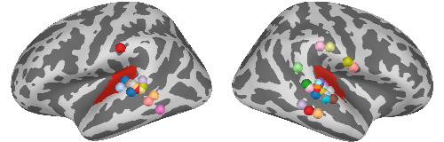
(a) SURE.

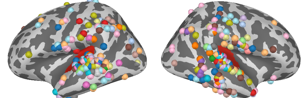
(b) Spatial CV.

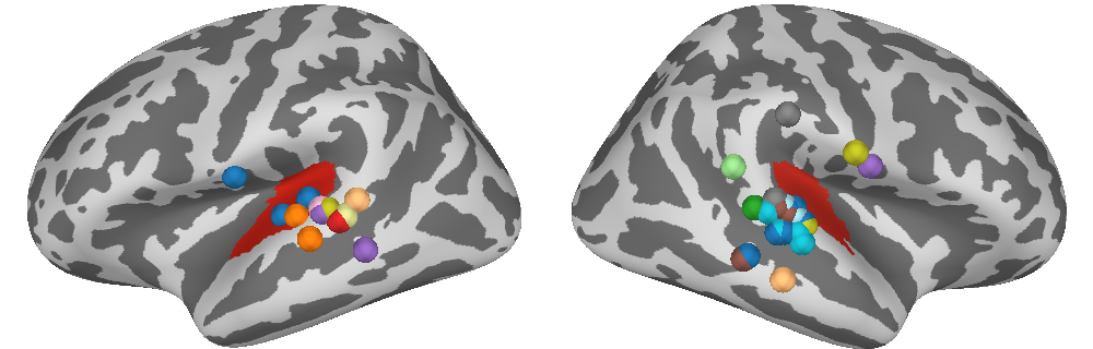
(c) $\lambda$-MAP.

Figure 2: Real data, brain source locations aggregated across subjects. Brain source locations reconstructed in each hemisphere after an auditory stimulation for each model selection procedure.

Table 1: Real data, aggregated results.

Average metrics	Spatial CV	SURE	$\lambda$-MAP
$\lambda/\lambda_{\text{max}}$	0.30	0.61	0.9
Explained variance	0.67	0.32	0.06
# of sources	9.30	1.44	1.3
% of zero sources	0	0	29.63
% of one source	0	55.56	40.74
% of two sources	3.7	44.44	18.52
% of $>2$ sources	96.3	0	11.11

4 Broader impact

This paper paves the way to a wider adoption of recent results in machine learning in the context of non-invasive brain source imaging commonly employed in cognitive and clinical neuroscience. Since the code is already available in the MNE package, the proposed algorithm could soon be impactful in the neuroimaging community.

Appendix A MxNE

We recall that $\mathbf{G}\in\mathbb{R}^{N\times P}$ denotes the design matrix, $\mathbf{M}\in\mathbb{R}^{N\times T}$ is the measurement matrix. Given a regularization parameter $\lambda>0$, the MxNE optimization problem [Gramfort et al., 2012] reads:

$$\widehat{\mathbf{X}}^{(\lambda)}\in\operatorname*{arg\,min}_{\mathbf{X}\in\mathbb{R}^{P\times T}}\frac{1}{2}\lVert\mathbf{M-GX}\rVert^{2}_{\text{F}}+\lambda\sum_{s=1}^{S}\lVert\mathbf{X}_{s}\rVert_{\mathrm{F}}\enspace.$$ (4)

It relies on a convex optimization problem that can be solved using block coordinate descent solvers [Tseng and Yun, 2009, Shi et al., 2016, Massias et al., 2020].

Appendix B Algorithms details

B.1 FDMC SURE

Evaluating the FDMC SURE consists in solving the following bilevel optimization problem [Deledalle et al., 2014]:

$$\begin{split}&\hat{\lambda}\in\operatorname*{arg\,min}_{\lambda\in\mathbb{R}}\frac{1}{2}\lVert\mathbf{M}-\mathbf{G}\widehat{\mathbf{X}}^{(\lambda,1)}\rVert^{2}_{\text{F}}+\frac{2\sigma^{2}}{\epsilon}\langle\mathbf{G}(\widehat{\mathbf{X}}^{(\lambda,2)}-\widehat{\mathbf{X}}^{(\lambda,1)}),\mathbf{\Delta}\rangle\\ \text{s.t.}\enspace&\widehat{\mathbf{X}}^{(\lambda,1)}\in\operatorname*{arg\,min}_{\mathbf{X}\in\mathbb{R}^{P\times T}}\frac{1}{2}\lVert\mathbf{M}-\mathbf{GX}\rVert^{2}_{\text{F}}+\lambda\sum_{s=1}^{S}\sqrt{\lVert\mathbf{X}_{s}\rVert_{\mathrm{F}}}\\ &\widehat{\mathbf{X}}^{(\lambda,2)}\in\operatorname*{arg\,min}_{\mathbf{X}\in\mathbb{R}^{P\times T}}\frac{1}{2}\lVert\mathbf{M}+\epsilon\mathbf{\Delta}-\mathbf{GX}\rVert^{2}_{\text{F}}+\lambda\sum_{s=1}^{S}\sqrt{\lVert\mathbf{X}_{s}\rVert_{\mathrm{F}}}\enspace,\end{split}$$ (5)

with $\epsilon>0$ and $\mathbf{\Delta}\in\mathbb{R}^{N\times T}$ a matrix which coefficients are independent and identically distributed from a normal distribution of mean $0$ and of variance $1$. Since data is assumed to be whitened, $\sigma$ is set to $1$. The finite difference step $\epsilon$ is chosen using the heuristic from Deledalle et al. [2014]: $\epsilon=\frac{2\sigma}{N^{0.3}}$. Alg. 1 shows how to solve the inner problem of LABEL:eq:bilevel_sure_mcfd. The computation of the FDMC SURE can be found in Alg. 2. Below $\odot$ stands for the element-wise multiplication. input : $\mathbf{G}\in\mathbb{R}^{N\times P},\mathbf{M}\in\mathbb{R}^{N\times T},\lambda>0,K\in\mathbb{N}$ init : $\widetilde{\mathbf{X}}=\mathbf{0}_{\mathbb{R}^{P\times T}},\mathbf{W}=\mathbf{I}_{P},\mathbf{w}=\mathbf{0}_{S}$ $\epsilon=10^{-8}$ for $k=1,\dots,K$ do        $\widetilde{\mathbf{G}}=\mathbf{G}\mathbf{W}$       // Iteratively solve convex problems        $\widetilde{\mathbf{X}}\leftarrow$ $\texttt{MxNE}(\widetilde{\mathbf{G}},\mathbf{M})$ ;         // Using $\widetilde{\mathbf{X}}$ to warm start              $\mathbf{X}=\mathbf{W}\widetilde{\mathbf{X}}$       $\mathbf{w}=((2\lVert\mathbf{X}_{s}\rVert_{\text{F}}+\epsilon)^{-1})_{s\in[S]}$       $\mathbf{W}=\text{diag}(\mathbf{w}\otimes\mathbf{1}_{(3)})$ return $\mathbf{X}$ Algorithm 1 irMxNE [Strohmeier et al., 2016]

input : $\mathbf{G}\in\mathbb{R}^{N\times P},\mathbf{M}\in\mathbb{R}^{N\times T},\lambda>0,K\in\mathbb{N}$ init : $\mathbf{\Delta}\in\mathbb{R}^{N\times T},\epsilon>0,\sigma>0$ $\forall(n,t)\in[n]\times[T],\mathbf{\Delta}_{n,t}\sim\mathcal{N}(0,1)$ $\mathbf{X}^{(\lambda,1)}\leftarrow$ Alg. 1$(\mathbf{G},\mathbf{M},\lambda,K)$ $\mathbf{X}^{(\lambda,2)}\leftarrow$ Alg. 1$(\mathbf{G},\mathbf{M}+\epsilon\Delta,\lambda,K)$ // Degree of freedom computation $\mathbf{J}=\mathbf{G}(\mathbf{X}^{(\lambda,2)}-\mathbf{X}^{(\lambda,1)})\odot\mathbf{\Delta}$ // Finite-difference $\text{dof}=\frac{1}{\epsilon}\sum_{i=1}^{N}\sum_{j=1}^{T}\mathbf{J}_{i,j}$ // FDMC SURE computation $\mathrm{SURE}=\lVert\mathbf{M}-\mathbf{G}\mathbf{X}^{(\lambda,1)}\rVert^{2}_{\text{F}}-NT\sigma^{2}+2\sigma^{2}\text{dof}$ return $\mathrm{SURE}$

(adapted from Deledalle et al. [2014])

Algorithm 2 Compute FDMC SURE

(adapted from Deledalle et al. [2014])

Combining both algorithms, we propose in Alg. 3 the procedure to automatically select $\lambda>0$ for irMxNE.

input : $\mathbf{G}\in\mathbb{R}^{N\times P},\mathbf{M}\in\mathbb{R}^{N\times T},\lambda_{1},\dots,\lambda_{n}>0,K\in\mathbb{N}$

init : $\mathrm{SURE}_{\mathrm{opt}}=+\infty$

for $\lambda=\lambda_{1},\dots,\lambda_{n}$ do

       $\mathrm{SURE}\leftarrow$Alg. 2$(\mathbf{G},\mathbf{M},\lambda,K)$

      if $\mathrm{SURE}<\mathrm{SURE}_{\mathrm{opt}}$ then

             $\lambda_{\mathrm{opt}}=\lambda$; $\mathrm{SURE}_{\mathrm{opt}}=\mathrm{SURE}$

return $\lambda_{\mathrm{opt}}$

Algorithm 3 Grid-search to solve Problem LABEL:eq:bilevel_sure_mcfd

B.2 Cross-validation

Cross-validation consists in partitioning data $(\mathbf{G},\mathbf{M})$ into $V\in\mathbb{N}^{*}$ hold-out datasets $(\mathbf{G}^{\text{train}_{v}},\mathbf{M}^{\text{train}_{v}})$, $v\in[V]$. The matrices are partitioned along the row axis, a setup referred to as spatial cross-validation when dealing with M/EEG data. The regularization parameter $\lambda$ is then chosen to minimize the averaged squared norm of the errors:

$$\begin{split}&\hat{\lambda}\in\operatorname*{arg\,min}_{\lambda\in\mathbb{R}}\frac{1}{V}\sum_{v=1}^{V}\lVert\mathbf{M}^{\text{val}_{v}}-\mathbf{G}^{\text{val}_{v}}\widehat{\mathbf{X}}^{(\lambda,v)}\rVert^{2}_{\text{F}}\\ \text{s.t.}\enspace&\widehat{\mathbf{X}}^{(\lambda,v)}\in\operatorname*{arg\,min}_{\mathbf{X}\in\mathbb{R}^{P\times T}}\frac{1}{2}\lVert\mathbf{M}^{\text{train}_{v}}-\mathbf{G^{\text{train}_{v}}X}\rVert^{2}_{\text{F}}+\lambda\sum_{s=1}^{S}\sqrt{\lVert\mathbf{X}_{s}\rVert_{\mathrm{F}}}\quad,\quad\forall v\in[V]\enspace.\end{split}$$ (6)

B.3 Hierarchical Bayesian modelling

input : $\mathbf{G}\in\mathbb{R}^{N\times P},\mathbf{M}\in\mathbb{R}^{N\times T},\lambda^{(0)}\in\mathbb{R}^{+},n_{\mathrm{iter}}\in\mathbb{N}^{*},\beta>0,\epsilon>0$

init : $\lambda_{\max}=\lVert\mathbf{G}^{\top}\mathbf{M}\rVert_{2,\infty}$, $m=\lambda_{\max}/2$, $\alpha=m\beta+1$

for $i=1,\dots,n_{\mathrm{iter}}$ do

       $\mathbf{X}\leftarrow$ Alg. 1 ( $\mathbf{G}$, $\mathbf{M}$, $\lambda^{(i-1)}$) // Solve ixMxNE problem

      

      $\lambda^{(i)}=(2ST+\alpha-1)/(\sum_{s=1}^{S}\sqrt{\lVert\mathbf{X}_{s}\rVert_{\mathrm{F}}}+\beta)$

      if $\lvert\lambda^{(i)}-\lambda^{(i-1)}\rvert<\epsilon$ then

             return $\lambda^{(i)}$

return $\lambda^{n_{\mathrm{iter}}}$

Algorithm 4 $\lambda$-MAP [Bekhti et al., 2017]

For $\lambda$-MAP, we had to fine-tune by hand the hyperprior parameter. We set $\beta=10$ for simulated data, and $\beta=5$ for real data. While $\lambda$-MAP is robust to the initialization of $\lambda$, it remains highly dependent of $\beta$, making it not fully automatic. Some experiments required an order of magnitude larger $\beta$ to prevent the iterate scheme to converge over $\lambda_{\text{max}}$. Indeed, we have noticed that $\lambda$-MAP often selects a hyperparameter $\lambda$ larger than $\lambda_{\text{max}}$, due to a poorly-chosen $\beta$.

B.4 Warm start

To accelerate the grid-search procedure, we sequentially solve the first convex subproblems (before the first reweighting) and initialize the weights of the $i$-th Lasso estimator $\widehat{\mathbf{X}}^{(\lambda_{i})}$ with $\widehat{\mathbf{X}}^{(\lambda_{i-1})}$. This computational trick is known as warm start (Alg. 5).

input : $\mathbf{G}\in\mathbb{R}^{N\times P},\mathbf{M}\in\mathbb{R}^{N\times T},\lambda_{1},\dots,\lambda_{n}>0,K\in\mathbb{N}^{*}$

init : $\mathbf{X}^{(\lambda_{0})}=\textbf{0}_{N\times T}$

// First solve problems without reweighting

for $i\in[n]$ do

       // This leads a more efficient warm start

       $\mathbf{X}^{(\lambda_{i})}\leftarrow\texttt{MxNE}(\mathbf{G},\mathbf{M},\lambda_{i})$ ;

       // Solve MxNE using $\mathbf{X}^{(\lambda_{i-1})}$ to warm start

      

// Then solve the remaining subproblems

for $i\in[n]$ do

       $\mathbf{X}^{(\lambda_{i})}\leftarrow\texttt{irMxNE}(\mathbf{G},\mathbf{M},\lambda_{i},K-1)$ ;

       // Solve irMxNE using $\mathbf{X}^{(\lambda_{i})}$ to warm start

      

return $\mathbf{X}^{(\lambda_{1})},\dots,\mathbf{X}^{(\lambda_{n})}$

Algorithm 5 Efficient warm start for reweighted Lasso with grid-search

References

- Akiba et al. [2019] T. Akiba, S. Sano, T. Yanase, T. Ohta, and M. Koyama. Optuna: A next-generation hyperparameter optimization framework. 2019.
- Arlot and Celisse [2010] S. Arlot and A. Celisse. A survey of cross-validation procedures for model selection. Statistics surveys, 4:40–79, 2010.
- Baillet et al. [2001] S. Baillet, J.C. Mosher, and R.M. Leahy. Electromagnetic brain mapping. IEEE Signal Processing Magazine, 18(6):14–30, 2001. doi: 10.1109/79.962275.
- Bekhti et al. [2017] Y. Bekhti, R. Badeau, and A. Gramfort. Hyperparameter Estimation in Maximum a Posteriori Regression Using Group Sparsity with an Application to Brain Imaging. 25th European Signal Processing Conference (EUSIPCO) , pages 256–260, 2017.
- Bekhti et al. [2018] Y. Bekhti, F. Lucka, J. Salmon, and A. Gramfort. A hierarchical bayesian perspective on majorization-minimization for non-convex sparse regression: application to M/EEG source imaging. Inverse Problems, 34(8):085010, 2018. doi: 10.1088/1361-6420/aac9b3. URL https://doi.org/10.1088/1361-6420/aac9b3.
- Berger [1929] H. Berger. Über das elektroenkephalogramm des menschen. Archiv für psychiatrie und nervenkrankheiten, 87(1):527–570, 1929.
- Bergstra and Bengio [2012] J. Bergstra and Y. Bengio. Random search for hyper-parameter optimization. Journal of Machine Learning Research, 2012.
- Bertrand et al. [2020] Q. Bertrand, Q. Klopfenstein, M. Blondel, S. Vaiter, A. Gramfort, and J. Salmon. Implicit differentiation of Lasso-type models for hyperparameter optimization. ICML, 2020.
- Bertrand et al. [2021] Q. Bertrand, Q. Klopfenstein, M. Massias, M. Blondel, S. Vaiter, A. Gramfort, and J. Salmon. Implicit differentiation for fast hyperparameter selection in non-smooth convex learning. arXiv preprint arXiv:2105.01637, 2021.
- Blu and Luisier [2007] T. Blu and F. Luisier. The SURE-LET approach to image denoising. IEEE Trans. Image Process., 16(11):2778–2786, 2007.
- Candès et al. [2008] E. J. Candès, M. B. Wakin, and S. P. Boyd. Enhancing sparsity by reweighted minimization. J. Fourier Anal. Applicat., 14(5-6):877–905, 2008.
- Chevalier et al. [2018] J.-A. Chevalier, J. Salmon, and B. Thirion. Statistical inference with ensemble of clustered desparsified lasso. MICCAI, 2018.
- Cohen [1968] D. Cohen. Magnetoencephalography: evidence of magnetic fields produced by alpha-rhythm currents. Science, 161(3843):784–786, 1968.
- Colson et al. [2007] B. Colson, P. Marcotte, and G. Savard. An overview of bilevel optimization. Annals of operations research, 153(1):235–256, 2007.
- Craven and Wahba [1979] P. Craven and G. Wahba. Smoothing noisy data with spline functions: estimating the correct degree of smoothing by the method of generalized cross-validation. 1979.
- Dale and Sereno [1993] A. M. Dale and M. I. Sereno. Improved localizadon of cortical activity by combining eeg and meg with mri cortical surface reconstruction: A linear approach. Journal of cognitive neuroscience, 5:162—176, 1993. doi: 10.1162/jocn.1993.5.2.162.
- Deledalle et al. [2014] C.-A. Deledalle, S. Vaiter, J. Fadili, and G. Peyré. Stein Unbiased GrAdient estimator of the Risk (SUGAR) for multiple parameter selection. SIAM J. Imaging Sci., 7(4):2448–2487, 2014.
- Efron [1986] B. Efron. How biased is the apparent error rate of a prediction rule? J. Amer. Statist. Assoc., 81(394):461–470, 1986.
- Engemann and Gramfort [2015] D. A. Engemann and A. Gramfort. Automated model selection in covariance estimation and spatial whitening of MEG and EEG signals. NeuroImage, 108:328 – 342, 2015. ISSN 1053-8119. doi: https://doi.org/10.1016/j.neuroimage.2014.12.040. URL http://www.sciencedirect.com/science/article/pii/S1053811914010325.
- Fischl [2012] B. Fischl. Freesurfer. Neuroimage, 62(2):774–781, 2012.
- Franceschi et al. [2017] L. Franceschi, M. Donini, P. Frasconi, and M. Pontil. Forward and reverse gradient-based hyperparameter optimization. In ICML, pages 1165–1173, 2017.
- Franceschi et al. [2018] L. Franceschi, P. Frasconi, S. Salzo, and M. Pontil. Bilevel programming for hyperparameter optimization and meta-learning. In ICML, pages 1563–1572, 2018.
- Gramfort et al. [2012] A. Gramfort, M. Kowalski, and M. Hämäläinen. Mixed-norm estimates for the M/EEG inverse problem using accelerated gradient methods. Phys. Med. Biol., 57(7):1937–1961, 2012.
- Gramfort et al. [2013] A. Gramfort, D. Strohmeier, J. Haueisen, M. S. Hämäläinen, and M. Kowalski. Time-frequency mixed-norm estimates: Sparse M/EEG imaging with non-stationary source activations. NeuroImage, 70:410–422, 2013.
- Gramfort et al. [2014] A. Gramfort, M. Luessi, E. Larson, D. A. Engemann, D. Strohmeier, C. Brodbeck, L. Parkkonen, and M. S. Hämäläinen. MNE software for processing MEG and EEG data. NeuroImage, 86:446 – 460, 2014. doi: http://dx.doi.org/10.1016/j.neuroimage.2013.10.027.
- Kunapuli [2008] G. Kunapuli. A bilevel optimization approach to machine learning. Rensselaer Polytechnic Institute, 2008.
- Li et al. [2017] L. Li, K. Jamieson, G. DeSalvo, A. Rostamizadeh, and A. Talwalkar. Hyperband: A Novel Bandit-Based Approach to Hyperparameter Optimization. Journal of Machine Learning Research, 2017.
- Massias et al. [2020] M. Massias, S. Vaiter, A. Gramfort, and J. Salmon. Dual extrapolation for sparse generalized linear models. Journal of Machine Learning Research, 2020.
- Mazumder et al. [2011] R. Mazumder, J. H. Friedman, and T. J. Hastie. SparseNet: coordinate descent with nonconvex penalties. J. Amer. Statist. Assoc., 106(495):1125–1138, 2011.
- Molina et al. [1999] R. Molina, A. K. Katsaggelos, and J. Mateos. Bayesian and regularization methods for hyperparameter estimation in image restoration. IEEE Trans. Image Process., 8(2):231–246, 1999.
- Obozinski et al. [2011] G. Obozinski, M. J. Wainwright, and M. Jordan. Support union recovery in high-dimensional multivariate regression. Ann. Statist., 39(1):1–47, 2011.
- Pereyra et al. [2015] M. Pereyra, J. M. Bioucas-Dias, and M. A. T. Figueiredo. Maximum-a-posteriori estimation with unknown regularisation parameters. 2015 23rd European Signal Processing Conference (EUSIPCO), pages 230–234, 2015. doi: 10.1109/EUSIPCO.2015.7362379.
- Pesquet et al. [2009] J. C. Pesquet, A. Benazza-Benyahia, and C. Chaux. A SURE Approach for Digital Signal/Image Deconvolution Problems. IEEE Transactions on Signal Processing, 57:4616–4632, 2009.
- Ramani et al. [2008] S. Ramani, T. Blu, and M. Unser. Monte-Carlo SURE: a black-box optimization of regularization parameters for general denoising algorithms. IEEE Trans. Image Process., 17(9):1540–1554, 2008.
- Sato et al. [2004] M. Sato, T. Yoshioka, S. Kajihara, K. Toyama, N. Goda, K. Doya, and M. Kawato. Hierarchical bayesian estimation for meg inverse problem. NeuroImage, 23(3):806–826, 2004.
- Shao [1993] J. Shao. Linear model selection by cross-validation. Journal of the American Statistical Association, 88(422):486–494, 1993.
- Shi et al. [2016] H.-J. M. Shi, S. Tu, Y. Xu, and W. Yin. A primer on coordinate descent algorithms. ArXiv e-prints, 2016.
- Stein [1981] C. M. Stein. Estimation of the mean of a multivariate normal distribution. Ann. Statist., 9(6):1135–1151, 1981.
- Stone and Ramer [1965] L. R. A. Stone and J.C. Ramer. Estimating WAIS IQ from Shipley Scale scores: Another cross-validation. Journal of clinical psychology, 21(3):297–297, 1965.
- Strohmeier et al. [2016] D. Strohmeier, Y. Bekhti, J. Haueisen, and A. Gramfort. The iterative reweighted Mixed-Norm Estimate for spatio-temporal MEG/EEG source reconstruction. IEEE Transactions on Medical Imaging, 2016.
- Taylor et al. [2017] J. R. Taylor, W. Nitin, C. Rhodri, A. Tibor, M. A. Shafto, Marie Dixon, Lorraine K. Tyler, Cam-CAN, and Richard N. Henson. The cambridge centre for ageing and neuroscience (cam-can) data repository: Structural and functional mri, meg, and cognitive data from a cross-sectional adult lifespan sample. NeuroImage, 144:262–269, 2017. ISSN 1053-8119. doi: https://doi.org/10.1016/j.neuroimage.2015.09.018.
- Tibshirani [1996] R. Tibshirani. Regression shrinkage and selection via the lasso. J. R. Stat. Soc. Ser. B Stat. Methodol., 58(1):267–288, 1996.
- Tipping [2001] M. E. Tipping. Sparse bayesian learning and the relevance vector machine. J. Mach. Learn. Res., 1:211–244, 2001. ISSN 1532-4435. doi: 10.1162/15324430152748236.
- Tseng and Yun [2009] P. Tseng and S. Yun. Block-coordinate gradient descent method for linearly constrained nonsmooth separable optimization. J. Optim. Theory Appl., 140(3):513, 2009.
- Vidal et al. [2020] A. F. Vidal, V. De Bortoli, M. Pereyra, and A. Durmus. Maximum likelihood estimation of regularization parameters in high-dimensional inverse problems: An empirical bayesian approach part i: Methodology and experiments. SIAM Journal on Imaging Sciences, 13(4):1945–1989, 2020. doi: 10.1137/20M1339829.