Multi-modal 3D Human Pose Estimation with 2D Weak Supervision in Autonomous Driving
Abstract
3D human pose estimation (HPE) in autonomous vehicles (AV) differs from other use cases in many factors, including the 3D resolution and range of data, absence of dense depth maps, failure modes for LiDAR, relative location between the camera and LiDAR, and a high bar for estimation accuracy. Data collected for other use cases (such as virtual reality, gaming, and animation) may therefore not be usable for AV applications. This necessitates the collection and annotation of a large amount of 3D data for HPE in AV, which is time-consuming and expensive.
In this paper, we propose one of the first approaches to alleviate this problem in the AV setting. Specifically, we propose a multi-modal approach which uses 2D labels on RGB images as weak supervision to perform 3D HPE. The proposed multi-modal architecture incorporates LiDAR and camera inputs with an auxiliary segmentation branch. On the Waymo Open Dataset [27], our approach achieves a relative improvement over camera-only 2D HPE baseline, and improvement over LiDAR-only model. Finally, careful ablation studies and parts based analysis illustrate the advantages of each of our contributions.
1 Introduction
3D Human Pose Estimation (3D HPE) for autonomous vehicles (AV) has received little attention in the academic community relative to other applications like animation, games, virtual reality (VR), or surveillance [43] despite its central role in AV. Arguably, this could be because 3D HPE in AV differs greatly from HPE in other scenarios. For one, AV requires HPE in outdoor environments and in 3D, which is not the case for animation or games which are not outdoor [35, 17] or surveillance which is not necessarily in 3D [6]. Secondly, sensor characteristics and placements for LiDAR follow different logic compared to other depth sensors like in games or VR [34, 40]. Thirdly, requirements for accuracy, real-time prediction and generalization over a wide variety of scenarios are also different. Animation, surveillance, games and VR have relatively lower bars for accuracy compared to AV where HPE is a critical component for the perception module.
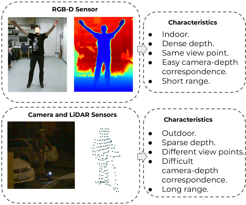
Diving deeper into the sensor, LiDAR differs from other depth sensors in several ways. Figure 1 summarizes these differences and gives visual illustrations. Firstly, LiDAR has longer range and larger FOV than RGB-D sensors, and it is more suitable for outdoor scenes. Point clouds from LiDAR are sparser and sweep a wider range of the environment. Secondly, LiDARs and cameras may not be co-located on AV platforms. Accurate registration is needed for correspondence between point clouds and image textures. Finally, failure cases for LiDAR caused by reflective materials, weather conditions, and dust on sensors differ from other sensor failures due to the difference in the physics of sensing as well as environmental factors.
Given the aforementioned differences and the evidence of 3D HPE models not generalizing across different datasets [43, 44, 37, 32] because of dataset bias, we see the need for developing approaches specific to AV that tackle the problem of 3D HPE. One straightforward way to tackle this problem would be to collect 3D human pose annotations for a large and diverse dataset of LiDAR point clouds in AV scenarios like the Waymo Open Dataset [27]. However, the ”in-the-wild” setting of 3D HPE for AV presents serious challenges to annotating training data at this scale, in terms of time, cost and coverage of long tail scenarios.
In this paper, we propose an approach to use widely available and easier to get 2D human pose annotations to drive 3D HPE in a weakly-supervised setting. While the weakly-supervised setting is not uncommon for 3D HPE [44], using LiDAR in the AV setting requires separate consideration for the reasons mentioned thus far. Figure 2 shows the idea of the proposed method. While we use PointNet [22]-inspired architecture as the main point cloud processing network, we cannot fuse camera and LiDAR imagery at the lower levels like in other settings [38] because of the sparsity of LiDAR. We propose a cascade architecture with a CNN-based camera network for 2D pose estimation. In addition, we add an auxiliary segmentation branch in the point network to introduce stronger supervision to each point via multi-task learning. This gives us an advantage in the ”in-the-wild” settings, as shown by the results on the Waymo Open Dataset (Table 1 and Table 3). In the rest of the paper, we show that pose estimation performance benefits from all these designs.
The main contributions of this paper are as follows:
-
•
We propose a multi-modal framework which fuses RGB camera images and LiDAR point clouds to exploit the texture information and geometry information for 3D pose estimation in challenging AV scenarios.
-
•
We train 3D pose estimation models by weak supervision from pure 2D labels, which makes the labeling stage much less expensive.
-
•
We introduce an auxiliary segmentation branch into the point network to improve 3D pose estimation performance via multi-task learning.
We review related work in Section 2, and follow it up with details about our approach in Section 3. Section 4 discusses detailed experiments with results on two large datasets, followed by ablation studies and performance analysis (refer to supplementary for additional results). Finally, we conclude in Section 5 with a discussion of avenues for improvement and future directions.
2 Related Work
In recent years, many methods have been introduced for 3D HPE [43], although hardly any work has addressed the AV scenario. Most take RGB or RGB-D images as inputs, and operate in monocular, multiview or video settings.
Monocular 3D HPE approaches like Tome et al. [30] take the simplest of inputs (monocular RGB images) and predict 3D keypoints using a multi-stage method. This classical approach of “lifting” 3D keypoints from 2D images has been recently done using deep learning[18], and in the past using a database of 3D skeletons [1, 24, 33]. Recent criticisms of this approach have focused on over-reliance on the underlying 2D estimator, and of generalization problems[2, 43]. Extending this approach temporally [5, 45, 2, 44] also has been attempted, but still underperforms approaches which use depth information (see [42], [43] table 11).
Depth based approaches also come in different flavors. Some, like Zimmermann et al., [48] use a VoxelNet based method on RGB-D images with 3D labels. Others might only use point clouds [29], add temporal consistency formulations [12], use a split and recombine approach [39], or generate large amounts of synthetic data followed by supervised learning strategy [15]. Semi-supervised approaches [19, 25, 20, 26] have also been recently attempted to deal with the long tail and ”in-the-wild” scenarios.
Weakly-supervised 3D Human Pose Estimation:
Besides the above fully- and semi-supervised methods which rely on at least a certain amount of 3D annotations, there are also weakly-supervised methods that use pure 2D annotations. Tripathi et al. [31] introduced a self-supervised method with teacher-student strategy on RGB sequences. Chen et al. [4] introduced a weakly-supervised method with cycle GAN[47]-like structure on pure 2D labels. Other weakly-supervised methods include [3, 14]. All the above methods are RGB-based, and do not involve the use of point clouds, while our method utilizes point clouds to help to improve the prediction accuracy.
Fürst et al. [8] proposed an end-to-end system for 3D detection and HPE for RGB and LiDAR in AV with pure 2D keypoint annotations. However, their work only includes evaluations for 2D HPE and projected 3D HPE, while our approach is evaluated with real 3D annotations.
Point Cloud-Based Approaches:
Point cloud-based approaches differ from HPE on traditional depth sensors in their ability to handle sparse 3D data [11]. PointNet [22] is a popular network for point cloud-based classification and segmentation, improved with hierarchical structures in [23] and utilized for 3D object detection on RGB-D [21], and hand pose estimation [9, 10]. Finally, Zhang et al. [41] proposed a weakly supervised point cloud-based method for 3D human pose estimation. However, their method requires 3D annotations and is only evaluated in indoor RGB-D datasets, while our method works on uncontrolled AV scenarios with pure 2D annotations.
3 Method
3.1 Problem Formulation
The 3D pose estimation problem can be described as follows. For each human subject in consideration, there are two modalities of data available: the point cloud and a camera image of the person. The point cloud , consists of LiDAR points from a single scan with -dimensional features. In this work, . The camera image is an RGB image. Assuming we have the extrinsics and intrinsics of the LiDAR and camera, for each point , its 3D world coordinates in the point cloud coordinate system and 2D coordinates in the image coordinate system are known. Given these inputs, the goal is to predict 3D coordinates of pose keypoints of the corresponding person. Note that LiDAR point clouds are usually sparse and lie on the surface of the object, while ground truth keypoints are defined inside the human body. Therefore, we cannot choose a subset of as the 3D pose of the person and approach 3D HPE in AV as a classification problem.
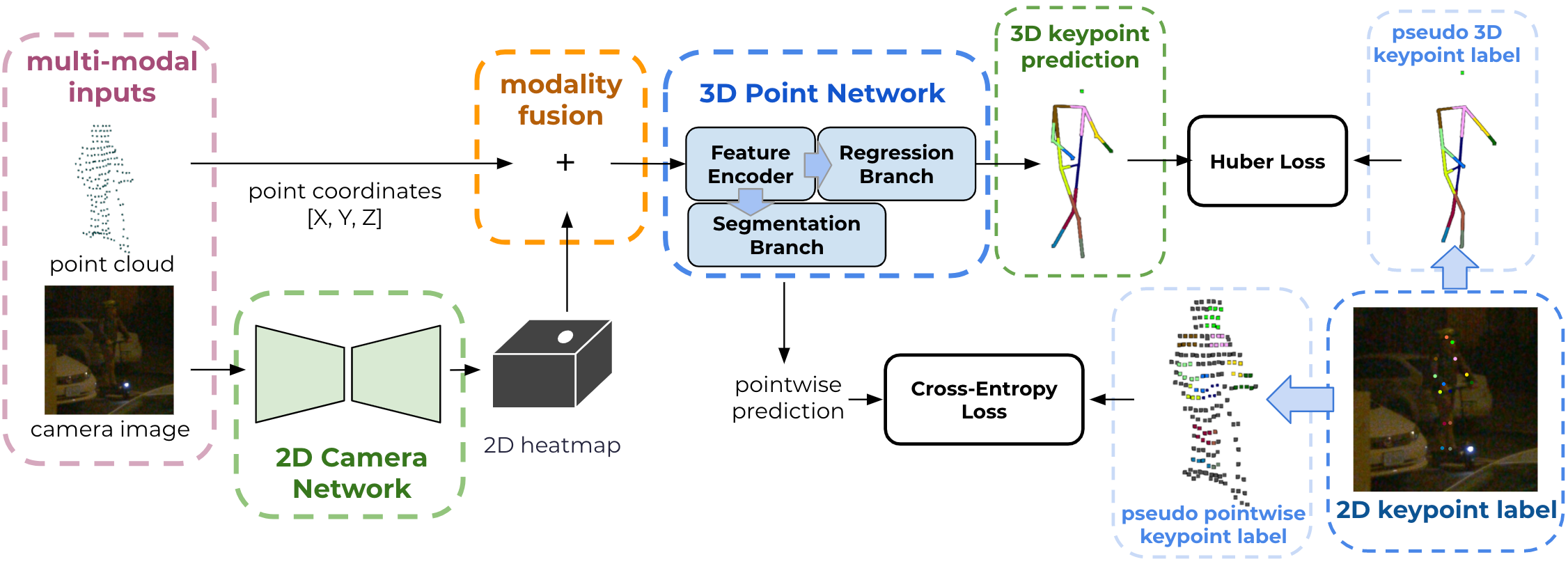
An overview of the proposed approach is shown in Figure 2. Our model is a cascade of a camera network and a point network. The camera network takes a 2D image as input and predicts a 2D keypoints heatmap[36]. This heatmap is used to augment the point cloud using modality fusion and fed into the point network. Finally, the regression branch of the point network predicts the 3D coordinates of keypoints. An auxiliary segmentation branch generates pointwise predictions which are only used for training. The model is trained on pseudo 3D labels and pointwise labels generated from 2D labels.
3.2 Modality Fusion of LiDAR and Camera
We introduce a 2D camera network with modality fusion to transfer texture information from RGB images to point clouds. Our camera network follows the architecture proposed in [36] which consists of a downscale module and an upscale module. The downscale module is a ResNet-50 network and the upscale module consists of three deconvolutional layers. A convolutional layer with sigmoid activation follows the upscale module and produces the output heatmap. The network takes an RGB image with size as input and generates a keypoint heatmap with size , where is the number of keypoints. Each pixel in the heatmap is a dimensional vector, indicating the likelihood of the corresponding image pixel belonging to each of the keypoints.
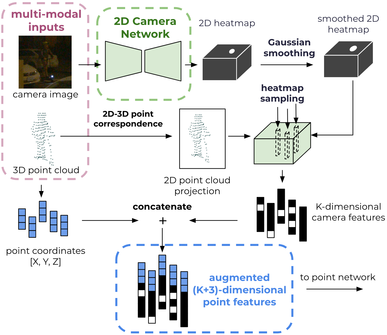
The heatmap is consequently sampled at points corresponding to the 2D projections on the camera image of 3D LiDAR points, to generate camera features as shown in Figure 3. The camera feature for point is computed as , which is a slice of at location . Here and , where are the 2D image coordinates of point . In practice, we observe that heatmaps from the camera network are usually very peaky, which contains little information at locations not close to any keypoints. Hence, we apply Gaussian smoothing to enlarge the receptive field at these locations [7], so the corresponding point can utilize the information from a larger neighborhood on the image.
Finally, camera features are concatenated with the original point feature to generate the augmented point cloud , which serves as the input of the following point network. This augmentation directly incorporates texture information from RGB images into the point cloud, which helps the LiDAR based point network with information useful for more accurate keypoint predictions. Similar concatenation can be found in [48], where voxel representations are concatenated with heatmaps before feeding into a VoxelNet [46].
The proposed cascade modality fusion architecture achieves improvements because heatmap predictions from the camera network carry complementary texture related semantic cues that are not present in LiDAR point features. Therefore, augmenting lower-level LiDAR point features with higher-level camera features provides the point network both low- and high- level point cloud information. By introducing modality fusion, we achieve relative improvement on the Waymo Open Dataset compared to the LiDAR-only baseline (Table 3 in Section 4).
3.3 Auxiliary Pointwise Segmentation Branch
Our point network is the primary component of the proposed method, which directly generates 3D keypoint prediction from augmented point clouds. The regression branch predicts a -dimensional output vector corresponding to the 3D coordinates of keypoints.
Even though rich camera information from the camera network is provided to the point network by modality fusion, the model’s designated output is still a fixed set of keypoints. It is difficult for a global regression loss to guide the point network to effectively utilize the camera information for each point. Therefore, to provide more direct supervision to every individual point, we propose an auxiliary segmentation branch after the feature encoder in the point network, inspired by the architecture of a segmentation PointNet [22]. For each LiDAR point, the segmentation branch predicts the pose keypoint it is closest to. In other words, the segmentation branch generates confidence scores for assigning LiDAR points to pose keypoints (a point with high score means that it is close to the corresponding keypoint). Here, the keypoint type for each point corresponds to the type of its nearest keypoint.
This additional point-wise loss helps the point network to digest more information from the camera network. By adding the auxiliary segmentation branch and loss, we achieve relative improvement on the Waymo Open Dataset compared to the modality-fusion architecture without the segmentation branch (Table 3 in Section 4).
3.4 Weakly-Supervised Model Training
Training the proposed point network with two branches needs two sets of labels: For the main regression branch, ground truth 3D keypoint coordinates are required; for the segmentation branch, pointwise keypoint type labels are needed. In the proposed method, we introduce a label generation method to enable model training on pure 2D labels for both tasks.
3.4.1 Label Generation
As stated in Section 3.1, we know the 3D coordinates of input points , their corresponding 2D image coordinates , and 2D ground truth keypoints . The correspondence is pre-computed by projecting 3D points onto the camera image coordinates according to the camera model. Since the projection is not a one-to-one mapping, directly back-projecting 2D labels to 3D space is impossible.
To generate 3D keypoint labels from the 2D labels and the point cloud, we make the following assumptions:
-
1.
the point cloud is dense enough so that there is at least one point in the neighborhood of each keypoint in 2D space;
-
2.
the human surface is smooth enough so that the depth does not rapidly change in the neighborhood of a keypoint;
-
3.
point cloud to camera registration is reliable.
Though point clouds will be downsampled to a fixed size before being fed into the point network, pseudo 3D labels are generated based on the point cloud before downsampling. Therefore, the above assumptions hold in most cases. Also, since LiDAR and camera are usually attached to the same rigid object (the vehicle) and are frequently calibrated, it is reasonable to assume that the registration is reliable.
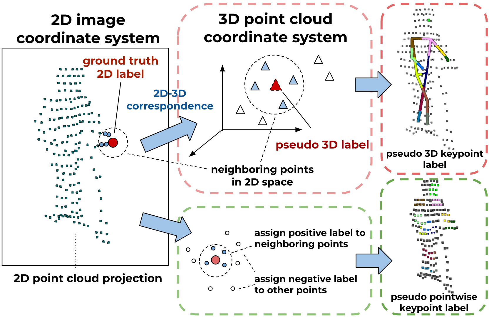
3D Keypoint Coordinates Label Generation: Based on our assumption, for each point in the point cloud, its accurate 2D projection on the camera image is known. Therefore, for a ground truth keypoint in 2D coordinates, we can first find its neighboring points in 2D space. Then, based on our assumptions, the depths of these points will be close enough to the true depth of the keypoint. As Figure 4, we use the average 3D coordinates of these neighboring points to approximate the coordinates of the keypoint,
| (1) |
Here weights the contribution of point to the pseudo keypoint based on their distances to the ground truth keypoint in 2D space, is the temperature that controls the softmax operation.
In case the pseudo 3D labels are not accurate, we also compute the reliability of the 3D approximation for each keypoint as , where is the temperature factor, to weight the losses on different keypoints during training.
Pointwise Keypoint Type Label Generation: To generate pointwise type labels for the segmentation task, we simply assign all neighboring points of a keypoint in 2D space to the corresponding keypoint type, shown in Figure 4. The type label for point with respect to keypoint is generated by
| (2) |
where is the neighboring radius for positive samples.
3.5 Training Losses
Point Network: The training loss for the regression branch is a Huber loss on the generated pseudo 3D labels, weighted by the reliability . The loss for the segmentation branch is a cross-entropy loss on the pseudo pointwise labels weighted by different positive/negative sample weights. The overall loss for the point network is
| (3) |
where is used to weight the auxiliary segmentation loss.
Camera Network: Similar to [36], the camera network is trained on a mean-squared-error loss with ground truth 2D heatmap. We train the camera network independently, then freeze it during point network training.
Note that we only train and evaluate on visible keypoints. During training, keypoint losses are only applied on visible keypoints, which means we will not generate pseudo labels for occluded keypoints. In Section 4, we show that even trained on visible keypoints only, the model is able to predict reasonable keypoints for occluded body parts. For more details of training losses, please refer to the supplementary material.
4 Experiments
4.1 Data and Evaluation Metrics
Training Data:
We collect an internal dataset with RGB images and LiDAR point clouds similar to the Waymo Open Dataset [27]. It consists of a total number of 197,381 pedestrians. These pedestrians are labeled with 2D keypoint labels of 13 keypoint types (nose, left/right shoulders, left/right elbows, left/right wrists, left/right hips, left/right knees and left/right ankles) in the camera image. These samples are split into a training set with 155,182 pedestrians and a test set with 42,199 pedestrians. The training set with pure 2D labels is used to train the proposed model.
3D Evaluation Data and Metrics:
The Waymo Open Dataset serves as our 3D evaluation set. It is composed of sensor data collected by Waymo cars under a variety of conditions. It contains 1,950 segments of 20s each, with sensor data including point clouds from LiDAR and RGB images captured by cameras. For 3D evaluation, we labeled 986 pedestrians with 3D keypoint coordinates of 13 keypoint types (same as our internal dataset) on LiDAR point clouds. We are looking to release these labels for evaluation once obtained related approvals.
Evaluation results are reported in the OKS (Object Keypoint Similarity) accuracy (OKS/ACC) metric, which is similar to the OKS/AP metric introduced in COCO keypoint challenge [16] (please refer to the supplementary material for more details), and MPJPE (Mean Per Joint Position Error) [13] in 3D coordinates.
2D Evaluation Data and Metrics:
The test set of our internal dataset serves as the 2D evaluation set. Evaluation results are reported in the OKS/ACC metric in 2D coordinates, after the 3D predictions are projected to 2D space by the corresponding lidar to camera projections.
Labeling:
For 2D/3D keypoint labeling on the Waymo Open Dataset and the Internal Dataset, we adopt a definition of keypoints similar to the COCO Challenge. Each keypoint is labeled by multiple annotators, whose results are aggregated to determine the final label. For 2D labeling, we only label 2D coordinates of keypoints that are visible in the camera image. For occluded keypoints, we label them as invisible. 3D labeling is similar, where we only label keypoints that are visible from the point clouds. Since we pair each LiDAR with its closest camera in location, the occlusion status of keypoints is mostly consistent between 2D and 3D.
| Methods | Waymo Open Dataset | Internal Dataset | |
|---|---|---|---|
| OKS@3D | MPJPE | OKS@2D | |
| camera-only [36] | 51.74% | 13.90cm | 78.19% |
| LiDAR-only | 59.58% | 10.80cm | 77.53% |
| multi-modal | 63.14% | 10.32cm | 82.94% |
| parts | camera-only | LiDAR-only | multi-modal | |||
| OKS@3D | OKS@2D | OKS@3D | OKS@2D | OKS@3D | OKS@2D | |
| nose | 24.50% | 75.10% | 23.83% | 56.27% | 29.74% | 72.17% |
| shoulder | 65.41% | 83.38% | 77.04% | 85.68% | 76.93% | 87.89% |
| elbow | 65.61% | 82.63% | 66.61% | 78.72% | 72.49% | 84.82% |
| wrist | 45.99% | 79.03% | 30.37% | 64.10% | 46.97% | 79.17% |
| hip | 57.69% | 87.97% | 79.42% | 90.33% | 74.76% | 92.37% |
| knee | 65.40% | 85.91% | 77.48% | 86.82% | 78.04% | 90.05% |
| ankle | 62.68% | 84.17% | 69.06% | 85.63% | 72.30% | 88.72% |
| overall | 51.74% | 78.19% | 59.58% | 77.53% | 63.14% | 82.94% |
| Configurations | Waymo Open Dataset | Internal Dataset | |||
| Reg. Loss | Seg. Loss | Camera | OKS@3D | MPJPE | OKS@2D |
| ✓ | 59.10% | 10.93cm | 77.52% | ||
| ✓ | ✓ | 59.58% | 10.80cm | 77.53% | |
| ✓ | ✓ | 62.03% | 10.53cm | 82.51% | |
| ✓ | ✓ | ✓ | 63.14% | 10.32cm | 82.94% |
Implementation Details:
For the Waymo Open Dataset and the Internal Dataset, we resize all camera images to , and randomly sub-sample the input point cloud to a fixed size of 256 points (we did not observe obvious performance gain for larger number of points). Please refer to the supplementary material for more training details.
4.2 Performance Analysis
To show the effectiveness of the proposed method, we compare with the following models.
Camera-only model: we use the same camera network [36] as the proposed method to predict 2D keypoints. Then 2D-to-3D keypoint lifting is implemented by the 2D-to-3D pseudo label generation method introduced in Section 3.4.1, the same way as we generate training labels.
LiDAR-only model: we use the proposed point network to predict 3D keypoints without the modality fusion, i.e. only use 3D coordinates of the point clouds as features.

Experimental results on two datasets are shown in Table 1. Table 2 further shows per-keypoint results. These results show that our method outperforms all baselines in the corresponding datasets. We also have the following observations.
Training on pseudo labels is effective. LiDAR-only baseline and the proposed method both outperform camera-only baseline on 3D metrics on the Waymo Open Dataset. Since the camera-only baseline is also trained on 2D labels and utilizes point clouds to lift the predictions to 3D space, the results indicate that it is more effective to directly train a 3D human pose model on pseudo labels generated from 2D ground truth.
Camera image improves 3D prediction. The proposed method performs better than LiDAR-only baseline on 3D metrics, which demonstrates that the information from 2D camera images helps 3D pose estimation. Table 2 shows that the proposed method outperforms baselines on almost all body parts. Compared to the LiDAR-only baseline, the margins are larger for difficult body parts like elbows or wrists, which shows that texture information from camera images is especially helpful for keypoints that are hard to localize.
Point cloud improves 2D prediction. LiDAR-only baseline has comparable performance with the camera-only baseline for 2D pose estimation on 2D metrics on the Internal Dataset. The proposed method surpasses the camera-only baseline, even if the models are not directly trained for 2D pose estimation. It shows that the depth information from 3D LiDAR point clouds also improves 2D pose estimation performance.
Modality fusion benefits from both modalities. The proposed method achieves the best performance on all metrics for both datasets. It proves that camera images and LiDAR point clouds provide complementary information, and modality fusion combines these sources of information to improve the overall performance.
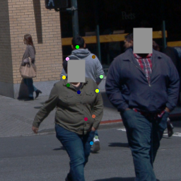
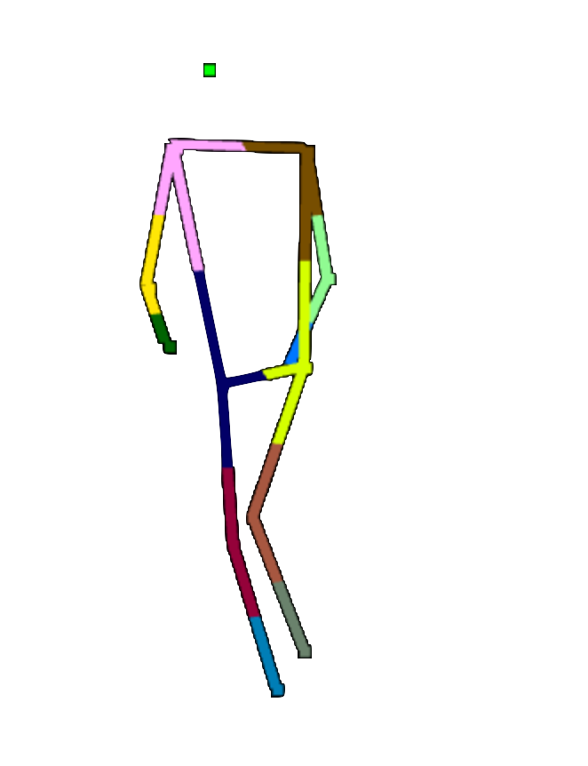
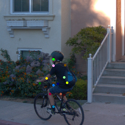
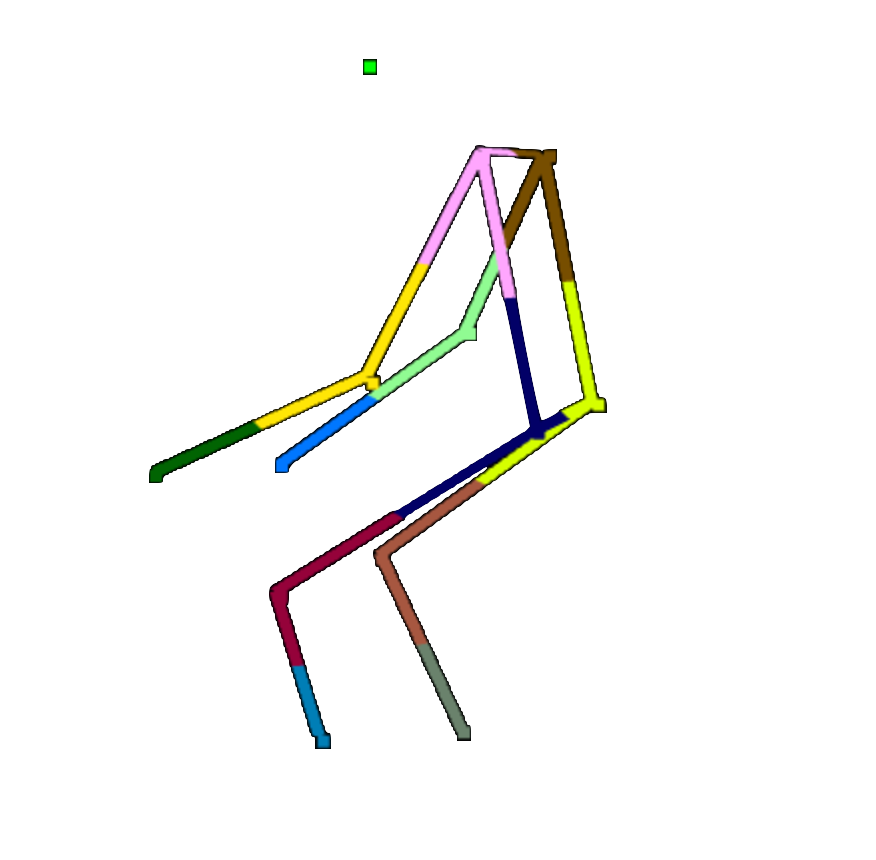
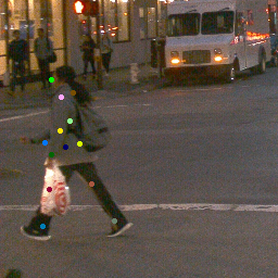
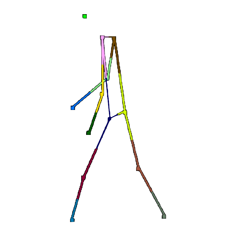
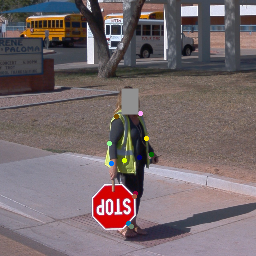
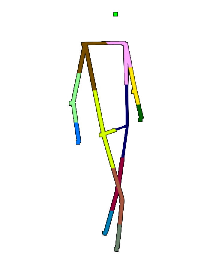
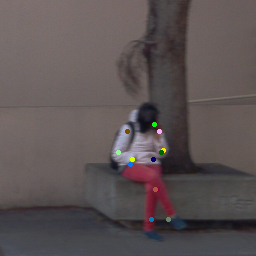
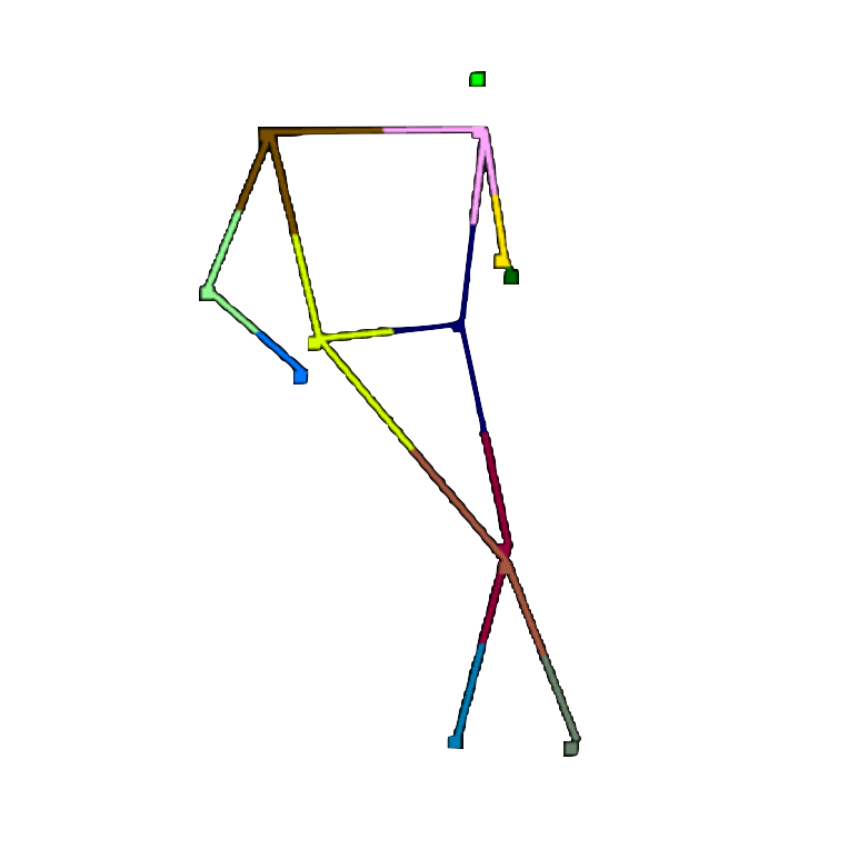
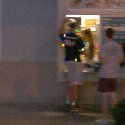
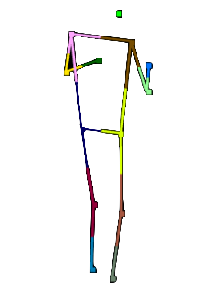
Figure 6 shows some qualitative results of the proposed method on the Waymo Open Dataset. In these examples, pedestrians are either occluded (6(a)), in an irregular pose (6(c), 6(i)), or carrying a large object (6(g), 6(e)). The proposed method accurately predicts the visible human keypoints and provides reasonable guesses for the occluded keypoints. Figure 6(k) is a failure case where the camera image is blurred because of the sensor motion. It causes an inaccurate prediction of the left wrist. More qualitative results can be found in the supplementary.
4.3 Ablation Studies
4.3.1 Ablation Study on Model Architecture
We conduct ablation studies to further demonstrate the effectiveness of our key designs: the auxiliary segmentation branch and the modality fusion with camera network. The results are shown in Table 3, where Reg. Loss means using regression loss (the primary loss) to train the point network, Seg. Loss means auxiliary segmentation branch being added (see Section 3.5), and Camera means using modality fusion with camera features. The results show that, by adding key features to the model, the performance improves consistently on all datasets. We also observe that the segmentation branch and modality fusion provide complementary improvements.
| Per-keypoint MPJPEs | Camera Network | ||||
|---|---|---|---|---|---|
| No camera | Inception 48x48 | Inception 64x64 | ResNet50 256x256 | ||
| all | 0.1080 | 0.1026 | 0.1028 | 0.1032 | |
| elbow | 0.1006 | 0.0940 | 0.0931 | 0.0891 | |
| wrist | 0.1652 | 0.1501 | 0.1473 | 0.1320 | |
| hip | 0.1081 | 0.1113 | 0.1113 | 0.1205 | |
| knee | 0.0944 | 0.0896 | 0.0910 | 0.0925 | |
| ankle | 0.1163 | 0.1100 | 0.1102 | 0.1107 | |
| nose | 0.0814 | 0.0762 | 0.0760 | 0.0837 | |
| shoulder | 0.0850 | 0.0814 | 0.0830 | 0.0872 | |
| Camera Network | Config | Waymo Open Dataset | Internal Dataset | ||
| Reg. | Seg. | OKS@3D | MPJPE | OKS@2D | |
| No Camera | ✓ | 59.10% | 10.93cm | 77.52% | |
| ✓ | ✓ | 59.58% | 10.80cm | 77.53% | |
| Inception 48x48 | ✓ | 61.12% | 10.51cm | 78.72% | |
| ✓ | ✓ | 62.22% | 10.26cm | 79.55% | |
| Inception 64x64 | ✓ | 61.05% | 10.46cm | 78.95% | |
| ✓ | ✓ | 62.52% | 10.28cm | 79.44% | |
| ResNet50 256x256 | ✓ | 62.03% | 10.53cm | 82.51% | |
| ✓ | ✓ | 63.14% | 10.32cm | 82.94% | |
4.3.2 Ablation Study on Camera Image Size and Camera Network Backbone
To study the effectiveness of modality fusion, experiments are conducted with different camera image sizes and camera network backbones with results in Table 5. Here Inception 48x48 uses an Inception[28]-inspired convolutional network backbone with a 48x48 image size; Inception 64x64 is similar to Inception 48x48 but with a 64x64 image size; ResNet50 256x256 is the ResNet50 backbone used in the proposed method with a 256x256 image size. From the results in Table 5, we observe that, even with smaller camera patch size and shallower backbone, the model still benefits from the additional camera modality. This observation is consistent with or without the auxiliary segmentation branch. With larger camera patch size and deeper backbone network, the overall performance is better.
We further studied the effect of different image sizes and network backbones on per-keypoint prediction errors in Table 4. These experiments are all with the proposed auxiliary segmentation branch. The results show that 1) Despite the choice of image size and backbone, addtional camera images generally bring considerable improvements on elbow, wrist, knee and ankle. This is because merely based on sparse and noisy LiDAR point clouds, accurately localizing these limb keypoints is difficult. Additional texture information from camera images makes the localization relatively easier. 2) Larger image size has better performance on most difficult keypoints like elbow and wrist. Surprisingly, it performs slightly worse than smaller patch sizes on other keypoints.
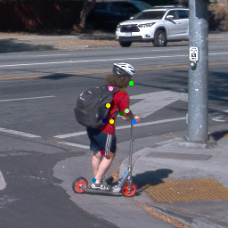
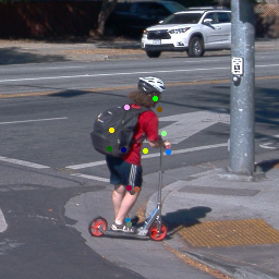
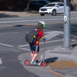
Figure 5 shows visualizations of 3D keypoint predictions on a pedestrian riding a scooter from the Waymo Open Dataset. It is a challenging case because of the objects (backpack, scooter) attached to the pedestrian and the irregular pose. The LiDAR-only model fails to predict accurate keypoints in Figure 5(a). By introducing modality fusion, improvements are observed on keypoints that are difficult to localize from sparse point clouds like those on the limbs (elbow, wrist, knee and ankle). The camera network used in the proposed method (ResNet50 on 256x256 images) predicts the most accurate keypoints (Figure 5(d)).
5 Conclusions
LiDAR based 3D HPE in AV differs from other applications for a variety of reasons including 3D resolution and range, absence of dense depth maps, and variation in test conditions. In this paper, we propose a multi-modal 3D HPE model with 2D weak supervision for autonomous driving. The model leverages both RGB camera images and LiDAR point clouds to tackle the challenges of 3D human pose estimation in unconstrained scenarios. Instead of using expensive 3D labels, the proposed model is trained on pure 2D labels. An auxiliary segmentation branch is added to introduce stronger supervision to the point network. Results on the Waymo Open Dataset (with evaluation labels to be released) and our internal dataset, and additional ablation studies showing the effectiveness of the proposed method.
References
- [1] Ijaz Akhter and Michael J. Black. Pose-conditioned joint angle limits for 3d human pose reconstruction. In IEEE Conf. Comput. Vis. Pattern Recog. (CVPR), pages 1446–1455, 2015.
- [2] Anurag Arnab, Carl Doersch, and Andrew Zisserman. Exploiting temporal context for 3d human pose estimation in the wild. IEEE Conf. Comput. Vis. Pattern Recog. (CVPR), 2019.
- [3] C. Chen and D. Ramanan. 3d human pose estimation = 2d pose estimation + matching. In IEEE Conf. Comput. Vis. Pattern Recog. (CVPR), pages 5759–5767, 2017.
- [4] Ching-Hang Chen, Ambrish Tyagi, Amit Agrawal, Dylan Drover, M. V. Rohith, Stefan Stojanov, and James M. Rehg. Unsupervised 3d pose estimation with geometric self-supervision. IEEE Conf. Comput. Vis. Pattern Recog. (CVPR), pages 5707–5717, 2019.
- [5] Yu Cheng, Bo Yang, Bo Wang, and Robby T. Tan. 3d human pose estimation using spatio-temporal networks with explicit occlusion training. In AAAI, 2020.
- [6] Srijan Das, Saurav Sharma, Rui Dai, Francois Bremond, and Monique Thonnat. Vpn: Learning video-pose embedding for activities of daily living, 2020.
- [7] Yang Feiyu, Song Zhan, Xiao Zhenzhong, Mo Yaoyang, Chen Yu, Pan Zhe, Zhang Min, Zhang Yao, Qian Beibei, and Jin Wu. Error compensation heatmap decoding for human pose estimation. IEEE Access, 9:114514–114522, 2021.
- [8] Michael Fürst, Shriya T. P. Gupta, René Schuster, Oliver Wasenmüller, and Didier Stricker. HPERL: 3d human pose estimation from RGB and lidar. Computing Research Repository, abs/2010.08221, 2020.
- [9] Liuhao Ge, Yujun Cai, Junwu Weng, and Junsong Yuan. Hand pointnet: 3d hand pose estimation using point sets. In IEEE Conf. Comput. Vis. Pattern Recog. (CVPR), 2018.
- [10] Liuhao Ge, Zhou Ren, and Junsong Yuan. Point-to-point regression pointnet for 3d hand pose estimation. In Eur. Conf. Comput. Vis. (ECCV), 2018.
- [11] Yulan Guo, Hanyun Wang, Qingyong Hu, Hao Liu, Li Liu, and Mohammed Bennamoun. Deep learning for 3d point clouds: A survey. IEEE Transactions on Pattern Analysis and Machine Intelligence, 43(12):4338–4364, 2021.
- [12] Mir Rayat Imtiaz Hossain and J. Little. Exploiting temporal information for 3d human pose estimation. In Eur. Conf. Comput. Vis. (ECCV), 2018.
- [13] Catalin Ionescu, Dragos Papava, Vlad Olaru, and Cristian Sminchisescu. Human3.6m: Large scale datasets and predictive methods for 3d human sensing in natural environments. IEEE Transactions on Pattern Analysis and Machine Intelligence, 36(7):1325–1339, jul 2014.
- [14] Muhammed Kocabas, Salih Karagoz, and Emre Akbas. Self-supervised learning of 3d human pose using multi-view geometry. IEEE Conf. Comput. Vis. Pattern Recog. (CVPR), pages 1077–1086, 2019.
- [15] Shichao Li, Lei Ke, Kevin Pratama, Yu-Wing Tai, Chi-Keung Tang, and Kwang-Ting Cheng. Cascaded deep monocular 3d human pose estimation with evolutionary training data. In IEEE Conf. Comput. Vis. Pattern Recog. (CVPR), June 2020.
- [16] Tsung-Yi Lin, Michael Maire, Serge Belongie, James Hays, Pietro Perona, Deva Ramanan, Piotr Dollár, and C. Lawrence Zitnick. Microsoft coco: Common objects in context. In Eur. Conf. Comput. Vis. (ECCV), pages 740–755, 2014.
- [17] Jingyuan Liu, Hongbo Fu, and Chiew-Lan Tai. Posetween: Pose-driven tween animation. In Proceedings of the 33rd Annual ACM Symposium on User Interface Software and Technology, UIST ’20, page 791–804, New York, NY, USA, 2020. Association for Computing Machinery.
- [18] Julieta Martinez, Rayat Hossain, Javier Romero, and James J. Little. A simple yet effective baseline for 3d human pose estimation. In Int. Conf. Comput. Vis. (ICCV), 2017.
- [19] Georgios Pavlakos, Xiaowei Zhou, and Kostas Daniilidis. Ordinal depth supervision for 3D human pose estimation. In IEEE Conf. Comput. Vis. Pattern Recog. (CVPR), 2018.
- [20] Dario Pavllo, Christoph Feichtenhofer, David Grangier, and Michael Auli. 3d human pose estimation in video with temporal convolutions and semi-supervised training. In IEEE Conf. Comput. Vis. Pattern Recog. (CVPR), 2019.
- [21] Charles R. Qi, Wei Liu, Chenxia Wu, Hao Su, and Leonidas J. Guibas. Frustum pointnets for 3d object detection from rgb-d data. In IEEE Conf. Comput. Vis. Pattern Recog. (CVPR), June 2018.
- [22] Charles R Qi, Hao Su, Kaichun Mo, and Leonidas J Guibas. Pointnet: Deep learning on point sets for 3d classification and segmentation. arXiv preprint arXiv:1612.00593, 2016.
- [23] Charles R Qi, Li Yi, Hao Su, and Leonidas J Guibas. Pointnet++: Deep hierarchical feature learning on point sets in a metric space. arXiv preprint arXiv:1706.02413, 2017.
- [24] Varun Ramakrishna, Takeo Kanade, and Yaser Sheikh. Reconstructing 3d human pose from 2d image landmarks. In Andrew Fitzgibbon, Svetlana Lazebnik, Pietro Perona, Yoichi Sato, and Cordelia Schmid, editors, Eur. Conf. Comput. Vis. (ECCV), pages 573–586, Berlin, Heidelberg, 2012. Springer Berlin Heidelberg.
- [25] Helge Rhodin, Mathieu Salzmann, and Pascal Fua. Unsupervised geometry-aware representation learning for 3d human pose estimation. In Eur. Conf. Comput. Vis. (ECCV), 2018.
- [26] H. Rhodin, Jörg Spörri, Isinsu Katircioglu, V. Constantin, F. Meyer, E. Müller, M. Salzmann, and P. Fua. Learning monocular 3d human pose estimation from multi-view images. IEEE Conf. Comput. Vis. Pattern Recog. (CVPR), pages 8437–8446, 2018.
- [27] Pei Sun, Henrik Kretzschmar, Xerxes Dotiwalla, Aurelien Chouard, Vijaysai Patnaik, Paul Tsui, James Guo, Yin Zhou, Yuning Chai, Benjamin Caine, Vijay Vasudevan, Wei Han, Jiquan Ngiam, Hang Zhao, Aleksei Timofeev, Scott Ettinger, Maxim Krivokon, Amy Gao, Aditya Joshi, Yu Zhang, Jonathon Shlens, Zhifeng Chen, and Dragomir Anguelov. Scalability in perception for autonomous driving: Waymo open dataset. In IEEE Conf. Comput. Vis. Pattern Recog. (CVPR), June 2020.
- [28] C. Szegedy, Wei Liu, Yangqing Jia, P. Sermanet, S. Reed, D. Anguelov, D. Erhan, V. Vanhoucke, and A. Rabinovich. Going deeper with convolutions. In IEEE Conf. Comput. Vis. Pattern Recog. (CVPR), pages 1–9, 2015.
- [29] Bugra Tekin, Pablo Marquez-Neila, Mathieu Salzmann, and Pascal Fua. Learning to fuse 2d and 3d image cues for monocular body pose estimation. In Int. Conf. Comput. Vis. (ICCV), pages 3961–3970, 10 2017.
- [30] Denis Tome, Chris Russell, and Lourdes Agapito. Lifting from the deep: Convolutional 3d pose estimation from a single image. In IEEE Conf. Comput. Vis. Pattern Recog. (CVPR), July 2017.
- [31] Shashank Tripathi, Siddhant Ranade, Ambrish Tyagi, and Amit Agrawal. Posenet3d: Unsupervised 3d human shape and pose estimation. 2020.
- [32] Bastian Wandt and Bodo Rosenhahn. Repnet: Weakly supervised training of an adversarial reprojection network for 3d human pose estimation. In IEEE Conf. Comput. Vis. Pattern Recog. (CVPR), June 2019.
- [33] Chunyu Wang, Yizhou Wang, Zhouchen Lin, Alan L. Yuille, and Wen Gao. Robust estimation of 3d human poses from a single image. In IEEE Conf. Comput. Vis. Pattern Recog. (CVPR), pages 2369–2376, 2014.
- [34] Chung-Yi Weng, Brian Curless, and Ira Kemelmacher-Shlizerman. Photo wake-up: 3d character animation from a single photo, 2018.
- [35] Nora S. Willett, Hijung Valentina Shin, Zeyu Jin, Wilmot Li, and Adam Finkelstein. Pose2Pose: Pose selection and transfer for 2D character animation. In 25th International Conference on Intelligent User Interfaces (IUI 2020), page 12, Mar. 2020.
- [36] Bin Xiao, Haiping Wu, and Yichen Wei. Simple baselines for human pose estimation and tracking. In Eur. Conf. Comput. Vis. (ECCV), 2018.
- [37] Wei Yang, Wanli Ouyang, Xiaolong Wang, Jimmy S. J. Ren, Hongsheng Li, and Xiaogang Wang. 3d human pose estimation in the wild by adversarial learning. IEEE Conf. Comput. Vis. Pattern Recog. (CVPR), pages 5255–5264, 2018.
- [38] Jiaming Ying and Xu Zhao. Rgb-d fusion for point-cloud-based 3d human pose estimation. In IEEE Int. Conf. Image Process. (ICIP), pages 3108–3112, 2021.
- [39] Ailing Zeng, X. Sun, F. Huang, Minhao Liu, Qiang Xu, and Stephen Lin. Srnet: Improving generalization in 3d human pose estimation with a split-and-recombine approach. Eur. Conf. Comput. Vis. (ECCV), abs/2007.09389, 2020.
- [40] Haotian Zhang, Cristobal Sciutto, Maneesh Agrawala, and Kayvon Fatahalian. Vid2player: Controllable video sprites that behave and appear like professional tennis players. ACM Trans. Graph., 40(3), may 2021.
- [41] Z. Zhang, L. Hu, X. Deng, and S. Xia. Weakly supervised adversarial learning for 3d human pose estimation from point clouds. IEEE Transactions on Visualization and Computer Graphics, 26(5):1851–1859, 2020.
- [42] Zhe Zhang, Chunyu Wang, Weichao Qiu, Wenhu Qin, and Wenjun Zeng. Adafuse: Adaptive multiview fusion for accurate human pose estimation in the wild. Int. J. Comput. Vis. (IJCV), pages 1–16, 2020.
- [43] Ce Zheng, Wenhan Wu, Taojiannan Yang, Sijie Zhu, Chen Chen, Ruixu Liu, Ju Shen, Nasser Kehtarnavaz, and Mubarak Shah. Deep learning-based human pose estimation: A survey. Computing Research Repository, abs/2012.13392, 2020.
- [44] Xingyi Zhou, Qixing Huang, Xiao Sun, Xiangyang Xue, and Yichen Wei. Towards 3d human pose estimation in the wild: A weakly-supervised approach. In Int. Conf. Comput. Vis. (ICCV), Oct 2017.
- [45] Xiaowei Zhou, Menglong Zhu, Spyridon Leonardos, Konstantinos G. Derpanis, and Kostas Daniilidis. Sparseness meets deepness: 3d human pose estimation from monocular video. In 2016 IEEE Conference on Computer Vision and Pattern Recognition (CVPR), pages 4966–4975, 2016.
- [46] Yin Zhou and Oncel Tuzel. Voxelnet: End-to-end learning for point cloud based 3d object detection, 2017.
- [47] Jun-Yan Zhu, Taesung Park, Phillip Isola, and Alexei A Efros. Unpaired image-to-image translation using cycle-consistent adversarial networks. In Int. Conf. Comput. Vis. (ICCV), 2017.
- [48] Christian Zimmermann, Tim Welschehold, Christian Dornhege, Wolfram Burgard, and Thomas Brox. 3d human pose estimation in rgbd images for robotic task learning. In IEEE International Conference on Robotics and Automation (ICRA), 2018.