Plasma model and Drude model permittivities
in Lifshitz formula

Abstract

At the physical level of rigour it is shown that there are no substantial theoretical arguments in favour of using either plasma mode permittivity or Drude model permittivity in the Lifshitz formula. The decision in this question rests with the comparison of theoretical calculations with the experiment. In the course of the study the derivation of the fluctuation-dissipation theorem is proposed where it is displayed clear at which reasoning stage and in what way the dissipation is taken into account. In particular it is shown how this theorem works in the case of the system with reversible dynamics, that is when dissipation is absent. Thereby it is proved that explicit assertion according to which this theorem is inapplicable to systems without dissipation is erroneous. The research is based on making use of the rigorous formalism of equilibrium two-time Green functions in statistical physics at finite temperature.

I Introduction

The problem of theoretical description of the Casimir forces [1] remains, as before, actual. To a certain extent that is promoted by accumulation of the experimental data in this field. At the beginning (Casimir, 1948) these forces were associated with the zero point oscillations of electromagnetic field in vacuum [2]. Later on (Lifshitz, 1955) a more broad physical base of these forces was revealed, namely, its close connection with electromagnetic fluctuations in material media was ascertained. This puts in the order of the day correct account of the material characteristics of the continuous media (first of all, its permittivity and permeability) in calculating the Casimir forces and employment here consistent mathematical methods (quantum field theory in media, fluctuation-dissipation theorem and others). The internal structure of the medium proves also to be important [3].

The substantial difficulties arise in these studies when trying to take into account the dissipative properties of the material. A few years ago it was found out that the experimental data on the Casimir forces are described enough good by the Lifshitz formula with the plasma model permittivity. An attempt to take into account the dissipation by substituting into the Lifshitz formula the Drude model permittivity makes worse the description of the experimental data (see, e.g., [4]). These topics were discussed in detail in many publications, we cite here only some of them [5, 6, 7, 8, 9]. There arose also certain difficulties in calculation of the Casimir entropy by making use of the Drude model permittivity [5, 6, 10, 11].

Such a situation turned out to be a surprise because the Drude model, taking account of dissipation, is more realistic in comparison with the plasma model which disregards dissipation. This gave rise to a rather long discussion (see papers cited above and references therein). As a result it became clear that it is needed a thorough examination of the physical and theoretical grounds used in derivation of the Lifshitz formula. It is this problem that is a subject of the present article.

One can distinguish two basic approaches to obtaining the Lifshitz formula. First of all the original approach used by Lifshitz himself should be noted [12, 13]. Below we argue that it is based substantially on the Callen-Welton fluctuation-dissipation theorem or simply FDT [14, 15, 16, 17]. Many authors have derived the Lifshitz formula by summing up the natural mode contributions to vacuum energy of the macroscopic electromagnetic filed in material media (the mode-by-mode summation or spectral summation, see, for example, [18] and references therein). This approach originates in the Casimir pioneering paper [19]. Such a summation wittingly assumes the real-valued frequencies. Therefore in this approach the media with dissipation cannot be treated because of their complex-valued permittivity, for example, the Drude model permittivity. Thus we have to concentrate ourselves on analysing the Lifshitz derivation of the formula in question.

Originally [12, 13] Lifshitz has obtained his famous formula in the framework of the semi-phenomenological fluctuational electrodynamics developed by Rytov [20, 21]. For the system in equilibrium, the Rytov technique amounts to the use of the Callen-Welton fluctuation-dissipation theorem [14, 15, 16, 17]. The proof of this equivalence has been done by Rytov himself [22, 21] and by the other authors [23, 24, 25].

In the Lifshitz approach there is an extremely complicated point, namely, the transition to the Matsubara imaginary frequencies $\omega\to i\zeta_{m},\quad\zeta_{m}=2\pi m({k_{\text{B}}T}/{\hbar}),\quad m=0,\pm 1,\pm 2,\dots$ and $k_{\text{B}}$ is the Boltzmann constant (the rotation of the integration path in the complex $\omega$ plane). Later on Lifshitz with coauthors [26, 27] repeated the derivation of the formula in question by making, from the very beginning, use of the very complicated formalism of quantum field theory in the statistical physics [28]. The central objects in this approach are the Matsubara Green functions at finite temperature, $\mathcal{D}_{ik}(\zeta_{n};\mathbf{r_{1},r_{2}})$, defined in terms of the retarded Green functions $D^{R}_{ik}(\omega,\mathbf{r_{1},r_{2}})$:

$$\mathcal{D}_{ik}(\zeta_{n};\mathbf{r_{1},r_{2}})=D^{R}_{ik}(i\zeta_{n},\mathbf{r_{1},r_{2}})\,{.}$$ (1)

Obviously in this approach the rotation of the integration contour is not required, however the equality (1) must be proved, in other words the transition to the Matsubara frequencies in the retarded Green functions (1) should be substantiated. It must be noted that in deriving the Lifshitz formula in Refs. [26, 27] the FDT is used also.

Thus in different derivations of the Lifshitz formula, which are of interest for the aim of the present paper, the employment of the FDT is a substantial step. That is why the main part of the present paper is devoted to revealing the requirements which should be satisfied for a correct application of the FDT when obtaining the Lifshitz formula. For this purpose, as a preliminary, the FDT is derived in a special way, namely, in two stages. At the first stage the so called averaged anticommutator-commutator relation is obtained which rigorously holds only for the Hamiltonian systems only. Then the linear response of the Hamiltonian system to the external action is calculated and the respective susceptibility is found. On this basis, as the second stage, the transition to the physical FDT is accomplished. Here we clear retrace in what way the phenomenological parameters describing dissipation are introduced into this theorem. Further we demonstrate conclusively that the requirements mentioned above are fulfilled if the plasma model permittivity is used and show to what extent they are violated when the Drude model permittivity is utilized.

The layout of the paper is the following. In Sec. II, we derive the averaged anticommutator-commutator relation within the framework of the Hamiltonian dynamics. In Sec. III, the linear response theory is considered for Hamiltonian systems exerted by external action and the respective susceptibility is obtained. In Sec. IV, the physical fluctuation-dissipation theorem is derived and its practical use is considered. In Sec.  V, we analyse the possibility to apply the plasma model and Drude model permittivities in the AC-relation and in the physical FDT. Preliminary we discuss the Lifshitz approach to description of the electromagnetic field in a material media. In Sec. VI, Conclusion, we formulate briefly the main inference of the paper, namely: there are no theoretical arguments in favour of using either plasma model permittivity or the Drude model permittivity in the Lifshitz formula. In Appendix A, we accomplish transition to the imaginary frequencies when deriving the Lifshitz formula with the plasma model permittivity at finite temperature.

II The averaged anti-commutator-commutator relation for Hamiltonian systems

The fluctuation-dissipation theorem [14, 17] connects the quantities characterizing spontaneous equilibrium fluctuations (equilibrium correlators) in the system with the generalized susceptibility specifying the linear response of the system to external action. As noted in the Introduction we derive FDT in two stages. As the first stage the averaged anticommutator-commutator relation (see below) is proved. We use the formalism of equilibrium two-times Green functions at finite temperature with real time in statistical physics [15, 16, 29, 30]. This formalism is based on the Hamiltonian description of the systems under study.

Let us consider a system in thermodynamic equilibrium state at the temperature $T$ which is described by a statistical operator, or density matrix, $\rho$:

$$\rho=Q^{-1}\exp(-\beta H),\quad Q=\operatorname{Tr\,}\exp(-\beta H),$$ (2)

where $H(q,p)$ is the Hamiltonian of the system and $\beta^{-1}=k_{\text{B}}T$. The averaging with respect to the equilibrium state will be denoted by braces

$$\langle\ldots\rangle=Q^{-1}\operatorname{Tr\,}(\rho\ldots)\,{.}$$ (3)

Let $A_{j}(q,p)$ is a classical dynamical variable and $A_{j}(t)$ is its Hermitian operator in the Heisenberg representation

$$A_{j}(t)=e^{\frac{i}{\hbar}Ht}A_{j}(0)\,e^{-\frac{i}{\hbar}Ht}{.}$$ (4)

We remind the derivation of the so called averaged anticommutator-commutator relation (AC-relation from now onwards) which expresses the symmetrized correlation function of the operators $A_{i}(t_{i}),\,A_{j}(t_{j})$

$$\{A_{i}(t_{i}),A_{j}(t_{j})\}\equiv\frac{1}{2}\,\left(\langle A_{i}(t_{i})A_{j}(t_{j})\rangle+\langle A_{j}(t_{j})A_{i}(t_{i})\rangle\right)$$ (5)

via the averaged values of the retarded commutator of these operators, i.e., in terms of the retarded Green function. For the sake of completeness we define at once the retarded and advanced Green functions

$$G_{ij}^{\,q}(t)\equiv\pm\,\frac{1}{i\hbar}\,\theta(\pm\,t)\langle[A_{i}(t_{i}),A_{j}(t_{j})]\rangle,\quad q=r,a,\quad t=t_{i}-t_{j}\,{.}$$ (6)

In this formula $\theta(t)$ is a step function, $\theta(t)=1$ for $t>0$ and $\theta(t)=0$ at $t<0$; the upper sings $(+)$ apply to the retarded Green function, $G^{\,r}(t)$, and the lower signs, $(-)$, concern the advanced Green function, $G^{\,a}(t)$. Below it will be shown that the Green functions (6), as well as the pair correlators, depend on the deference $t_{i}-t_{j}=t$.

Two-time temperature Green’s functions (6) are a direct generalization of the retarded and advanced Green functions introduced in quantum field theory (QFT) [31]. The distinction is only in the averaging method $\langle\ldots\rangle$. In QFT the averaging is conducted with respect to the ground state while in statistical mechanics the Gibbs distribution (2), (3) is used for this purpose.

From definition (6) we obtain in a straightforward way the following relations between the Green functions

$$G_{ij}^{r}(t)=G_{ji}^{a}(t),\qquad G_{ij}^{a}(t)=G_{ji}^{r}(t)$$ (7)

and their Fourier transforms

$$G_{ij}^{r}(\omega)=G_{ji}^{a}(\omega),\qquad G_{ij}^{a}(\omega)=G_{ji}^{r}(\omega)\,{,}$$ (8)

where

$$G^{q}_{ij}(t)=\int\limits_{-\infty}^{\infty}e^{-i\omega t}G^{q}_{ij}(\omega)\frac{d\omega}{2\pi}\,{,}\quad G^{q}_{ji}(t)=\int\limits_{-\infty}^{\infty}e^{-i\omega t}G^{q}_{ji}(\omega)\frac{d\omega}{2\pi}\,{;}{}$$

$$G^{q}_{ij}(\omega)=\int\limits_{-\infty}^{\infty}e^{i\omega t}G^{q}_{ij}(t)\,dt\,{,}\quad G^{q}_{ji}(\omega)=\int\limits_{-\infty}^{\infty}e^{i\omega t}G^{q}_{ji}(t)\,dt\,{,}\quad q=r,a.$$ (9)

In addition it is easy to show that the Green functions (6) for the Hermitian operators $A=A^{\dagger}$ are real functions of the time $t$

$$\left(G_{ij}^{q}(t)\right)^{*}=G_{ij}^{q}(t),\quad q=r,a\,{.}$$ (10)

From the last two equations (9) and definition (6) it follows, in particular, that the function $G^{r}_{ij}(\omega)$ has no singularities in the upper half-plane of the complex variable $\omega$ and $G^{a}_{ji}(\omega)$ in the lower half-plane $\omega$.

Further we shall use the spectral representations of the functions under consideration that are closely related with their Fourier transforms. Let $E_{\mu}$ and $C_{\mu}$ be the eigenvalues and eigenfunctions of the Hamiltonian $H$ in (2):

$$HC_{\mu}=E_{\mu}C_{\mu}\,{.}$$ (11)

Obviously, $C_{\mu}$ do not depend on $t$. By means of Eqs. (2)–(4) and (11) we get the spectral representation for the correlator

$$\langle A_{i}(t_{i})A_{j}(t_{j})\rangle=Q^{-1}\sum_{\nu,\mu}(C_{\nu}^{*}A_{i}(0)C_{\mu})(C_{\mu}^{*}A_{j}(0)C_{\nu})\,e^{-\beta E_{\nu}}e^{\frac{i}{\hbar}\,(E_{\nu}-E_{\mu})\,t},\quad t=t_{i}-t_{j}\,{.}$$ (12)

Thus the correlator function $\langle A_{i}(t_{i})A_{j}(t_{j})\rangle$ and, consequently, the Green function (6) depend on the deference $t_{i}-t_{j}=t$. Passing on to the Fourier transform

$$\langle A_{i}(t_{i})A_{j}(t_{j})\rangle=\int\limits_{-\infty}^{\infty}e^{-i\omega\,t}J_{ij}(\omega)\frac{d\omega}{2\pi}\,{,}$$ (13)

we deduce from (12) and (13)

$$J_{ij}(\omega)=\int\limits_{-\infty}^{\infty}e^{i\omega\,t}\langle A_{i}(t_{i})A_{j}(t_{j})\rangle\,dt=$$

$$=2\pi\,Q^{-1}\sum_{\nu,\mu}(C_{\nu}^{*}A_{i}(0)C_{\mu})(C_{\mu}^{*}A_{j}(0)C_{\nu})\,e^{-\beta E_{\nu}}\delta\left(\omega+\frac{E_{\nu}-E_{\mu}}{\hbar}\right){.}$$ (14)

Doing in the same way we obtain the spectral representation for the correlator with the transposed operators $\langle A_{j}(t_{j})A_{i}(t_{i})\rangle$:

$$\langle A_{j}(t_{j})A_{i}(t_{i})\rangle =Q^{-1}\sum_{\nu,\mu}(C_{\nu}^{*}A_{j}(0)C_{\mu})(C_{\mu}^{*}A_{i}(0)C_{\nu})\,e^{-\beta E_{\nu}}e^{\frac{i}{\hbar}\,(E_{\mu}-E_{\nu})\,t}$$ (15a)

$$=Q^{-1}\sum_{\nu,\mu}(C_{\nu}^{*}A_{i}(0)C_{\mu})(C_{\mu}^{*}A_{j}(0)C_{\nu})\,e^{-\beta E_{\mu}}e^{\frac{i}{\hbar}\,(E_{\nu}-E_{\mu})\,t},\quad t=t_{i}-t_{j}\,{.}$$ (15b)

The last equality (15b) is derived by interchanging the summation indexes $\nu\leftrightarrow\mu$ in (15a).

We define the Fourier transform of $\langle A_{j}(t_{j})A_{i}(t_{i})\rangle$ just as in Eq.  (13)

$$\langle A_{j}(t_{j})A_{i}(t_{i})\rangle=\int\limits_{-\infty}^{\infty}e^{-i\omega\,t}J_{ji}(\omega)\,\frac{d\omega}{2\pi}\,{,}\quad t=t_{i}-t_{j}\,{.}$$ (16)

In view of Eqs.  (16) and (15) we deduce the spectral density $J_{ji}(\omega)$

$$J_{ji}(\omega)=\int\limits_{-\infty}^{\infty}e^{i\omega\,t}\langle A_{j}(t_{j})A_{i}(t_{i})\rangle\,dt=$$

$$=2\pi Q^{-1}\sum_{\mu,\nu}(C^{*}_{\mu}A_{j}(0)C_{\nu})(C^{*}_{\nu}A_{i}(0)C_{\mu})\,e^{-\beta E_{\mu}}\delta\left(\omega+\frac{E_{\nu}-E_{\mu}}{\hbar}\right){.}$$ (17)

Taking into account the $\delta$-function in Eq.  (17) we can obviously do the substitution

$$\frac{E_{\mu}}{\hbar}=\frac{E_{\nu}}{\hbar}+\omega\,{.}$$

Comparison of transformed Eq.  (17) with Eq.  (14) yields an important relation

$$J_{ji}(\omega)=e^{-\beta\hbar\omega}J_{ij}(\omega)\,{.}$$ (18)

This property of the spectral density under consideration is in fact a direct consequence of the trivial equality which is satisfied by the density matrix (2) and the evolution operator $\exp(-\frac{i}{\hbar}\,H\,t)$ in (4) in the case of the Hamiltonian systems

$$\left.\exp\left(-\,\frac{i}{\hbar}\,H\,t\right)\right|_{t=-i\beta\hbar}=Q\,\rho=e^{-\beta H}\,{.}$$ (19)

With the help of (18) it is easy to derive the spectral density for the symmetrized correlator (5)

$$J_{\{ij\}}(\omega)=\int\limits_{-\infty}^{\infty}e^{i\,\omega\,t}\{A_{i}(t_{i}),A_{j}(t_{j}\}\,dt=\frac{1}{2}\,\left(J_{ij}(\omega)+J_{ji}(\omega)\right)=\frac{1}{2}\,J_{ij}(\omega)(1+e^{-\beta\hbar\omega})$$ (20)

and for the commutator $\langle[A_{i}(t_{i}),A_{j}(t_{j})]\rangle$

$$J_{[ij]}(\omega)=\int\limits_{-\infty}^{\infty}e^{i\,\omega\,t}\langle[A_{i}(t_{i}),A_{j}(t_{j})]\rangle\,dt=J_{ij}(\omega)(1-e^{-\beta\hbar\omega})\,{.}$$ (21)

The spectral density $J_{ij}(\omega)$ (14) for the Hermitian operators $A=A^{\dagger}$ possesses the property

$$J_{ij}(\omega)=J_{ji}^{*}(-\omega)\,{,}$$ (22)

which can be proved just as the equality (18). We shall not represent here this trivial proof.

Now we turn to the construction of the spectral density for the Green functions (6). For this it will be necessary the integral representation of the step function (6) (see, for example, [29, 30, 31]):

$$\theta(t)=\frac{i}{2\pi}\int\limits_{-\infty}^{\infty}d\omega\,\frac{e^{-i\omega\,t}}{\omega+i\varepsilon}\quad(\varepsilon>0,\;\varepsilon\to 0)\,{.}$$ (23)

With the help of Eqs. (6), (9), (21), and (23) we get

$$G^{q}_{ij}(\omega)=\int\limits_{-\infty}^{\infty}e^{i\omega\,t}G_{ij}^{q}(t)\,dt=\frac{1}{2\pi\hbar}\,\int\limits_{-\infty}^{\infty}d\omega^{\prime}J_{ij}(\omega^{\prime})\frac{e^{-\beta\hbar\omega^{\prime}}-1}{\omega^{\prime}-\omega\mp i\varepsilon}\,{,}\quad q=r,a\,{.}$$ (24)

In this formula, as well as in (6), the upper sign $(-)$ corresponds to $q=r$ and the lower sign, $(+)$, corresponds to $q=a$.

Previously we have noted that the Green functions for the Hermitian operators $A=A^{\dagger}$ are real functions of time (see Eq. (10)), therefore their Fourier transforms obey the relation

$$\left(G^{q}_{ij}(\omega)\right)^{*}=G^{q}_{ij}(-\omega),\quad q=r,a{;}$$

$${\operatorname{Re\,}}G^{q}_{ij}(\omega)={\operatorname{Re\,}}G^{q}_{ij}(-\omega)\,{,}\quad{\operatorname{Im\,}}G^{q}_{ij}(\omega)=-{\operatorname{Im\,}}G^{q}_{ij}(-\omega),\quad q=r,a.$$ (25)

This equality can be easily proved by utilizing Eqs.  (24) and (18), (22). Obviously this is a test of consistency of the Fourier transform definition used in Eqs. (9), (13), (14), (16), (17), (20), (21), and (24).

For our consideration the case is of a special interest when

$$A_{i}=A,\quad A_{j}=A^{\dagger}=A\,{.}$$ (26)

The point is the AC-relation can be derived in this case easily. Indeed, utilizing Eq. (14) one can show the spectral density $J_{AA^{\dagger}}(\omega)$ to be positive

$$J_{AA^{\dagger}}(\omega)=2\pi Q^{-1}\sum_{\mu,\nu}\left|(C_{\nu}^{*}A(0)C_{\mu})\right|^{2}e^{-\beta E_{\nu}}\delta\left(\omega+\frac{E_{\nu}-E_{\mu}}{\hbar}\right)>0\,{.}$$ (27)

By means of the known symbolic equality [31]

$$\frac{1}{x\pm i\varepsilon}={\cal P}\frac{1}{x}\mp i\pi\delta(x),\quad\varepsilon\to+0$$ (28)

we deduce from  (24)

$$G^{\,q}_{AA^{\dagger}}(\omega)= \frac{1}{2\pi\hbar}\int\limits_{-\infty}^{\infty}d\omega^{\prime}J_{AA^{\dagger}}(\omega^{\prime})(e^{-\beta\hbar\omega^{\prime}}-1){\cal{P}}\frac{1}{\omega^{\prime}-\omega}$$

$$\pm\frac{i}{2\hbar}J_{AA^{\dagger}}(\omega)(e^{-\beta\hbar\omega}-1),\quad q=r,a.$$ (29)

The spectral density $J_{AA^{\dagger}}(\omega)$ is real (see Eq. (27)), therefore it follows from Eq. (29)

$$\operatorname{Im\,}G^{\,q}_{AA^{\dagger}}(\omega)=\pm\frac{1}{2\hbar}J_{AA^{\dagger}}(\omega)(e^{-\beta\hbar\omega}-1),\quad q=r,a\,{,}$$ (30)

By making use of Eqs. (20) and (30) we obtain the spectral density of the symmetrized correlator $J_{\{AA^{\dagger}\}}(\omega)$:

$$J_{\{AA^{\dagger}\}}(\omega)=\mp\hbar\,\coth\left(\frac{\beta\hbar\omega}{2}\right)\operatorname{Im\,}G_{AA^{\dagger}}^{\,q}(\omega),\quad q=r,a\,{.}$$ (31)

Both signs in the right hand side of Eq. (31) lead to the same result because from Eq. (30) it follows

$$\operatorname{Im\,}G^{\,r}_{AA^{\dagger}}(\omega)=-\operatorname{Im\,}G^{\,a}_{AA^{\dagger}}(\omega)\,{.}$$

Therefore we have in the general case

$$J_{\{AA^{\dagger}\}}(\omega)=-\hbar\,\coth\left(\frac{\beta\hbar\omega}{2}\right)\operatorname{Im\,}G^{\,q}_{AA^{\dagger}}(\omega){,}\quad q=r,a\,{.}$$ (32)

Further we shall use the retarded Green function $(q=r)$ to conform our consideration to the general principle of causality, namely, cause precedes action.

Now we invert definition (20)

$$\{A(t_{i}),A^{\dagger}(t_{j}\}=\int\limits_{-\infty}^{\infty}e^{-i\,\omega\,t}J_{\{AA^{\dagger}\}}(\omega)\,\frac{d\omega}{2\pi}\,{,}\quad t=t_{i}-t_{j}$$ (33)

and substitute the spectral density $J_{\{AA^{\dagger}\}}(\omega)$ from (32) into (33) with $t_{i}=t_{j}=\tau$. As a result we get

$$\left.\{A(t_{i}),A^{\dagger}(t_{j})\}\right|_{t_{i}=t_{j}=\tau}\equiv\frac{1}{2}\,\left(\langle A(\tau)A^{\dagger}(\tau)\rangle+\langle A^{\dagger}(\tau)A(\tau)\rangle\right)$$

$$=-\frac{\hbar}{2\pi}\int\limits_{-\infty}^{\infty}d\omega\,\coth\left(\frac{\beta\hbar\omega}{2}\right)\operatorname{Im\,}G_{AA^{\dagger}}^{\,r}(\omega)=-\frac{\hbar}{\pi}\int\limits_{0}^{\infty}d\omega\,\coth\left(\frac{\beta\hbar\omega}{2}\right)\operatorname{Im\,}G_{AA^{\dagger}}^{\,r}(\omega){.}$$ (34)

At the last step in this equation we have taken into account that $\operatorname{Im\,}G_{AA^{\dagger}}^{\,r}(\omega)$ is an odd function (see Eq. (25)). In the first line of (34) averaging is carried out over the system at equilibrium. Hence the result does not depend on time $\tau$ and the correlator here can be denoted simply by $\langle A^{2}\rangle$.

Equation (34) expresses the symmetrized equilibrium correlator of the operators $A(\tau)$ and $A^{\dagger}(\tau)$, Eq. (5), in terms of the Fourier transform of the retarded Green function, i.e., through the retarded commutator of these operators. This formula is anticommutator-commutator relation mentioned before Eq.  (5) as a preliminary task in deriving FDT. It is important to note that this equation is exact and it is applicable only to the systems that admit the Hamiltonian description. In the course of derivation of this relation the system has been considered which is at the thermodynamical equilibrium.

Theoretically the exact AC-relation (34) may be used in both directions, namely, for finding the correlator of equilibrium fluctuations through retarded Green function as well as for obtaining this function via the respective correlator. Here it is assumed certainly that the Hamiltonian of the system under study is known. However the exact calculation of the left hand side and the right hand side in AC-relation (34) are the tasks of the same complexity level. Therefore the employment of this relation in such calculations does not give advantage. These difficulties are overcome in the physical FDT.

In order to proceed to derivation of the physical FDT we need the connection of the retarded Green function with the generalized susceptibility. In its turn this requires calculation of the linear response of the system under consideration to external action.

III The linear response of the Hamiltonian system
to external action

In the preceding Section we have derived the AC-relation Eq.  (34) considering equilibrium system at the temperature $T$ which is described by the Hamiltonian $H$ and the statistical operator $\rho$ (see Eqs. (2) and (3)). Now we find the linear response of this system to the external action [15, 16, 29, 30]. To this end we add to the Hamiltonian $H$ the following term

$$-\sum_{j}A_{j}F_{j}(t)\,{,}$$ (35)

where $A_{j}$ are, as before, the dynamical variables (operators) pertaining to the initial system and $F_{j}(t)$ are non-operator real functions describing external forces or fields. It is assumed that the fields $F_{j}(t)$ are adiabatically turned on in the remote past

$$F_{j}(t)\sim e^{\varepsilon t},\quad t\to-\infty,\quad\varepsilon>0\,{.}$$ (36)

Thus we are considering the system with a complete Hamiltonian

$$H^{\prime}_{t}=H-\sum_{j}A_{j}F_{j}(t)\,{.}$$ (37)

In this equation the subscript $t$ by the operator $H^{\prime}_{t}$ points to the explicit dependence of this Schrödinger operator on time due to the external fields. The corresponding statistical operator $\rho^{\prime}(t)$ is determined by the equation

$$i\hbar\,\frac{\partial\rho^{\prime}(t)}{\partial t}=[H^{\prime}_{t},\rho^{\prime}(t)]$$ (38)

with the initial condition

$$\left.\rho^{\prime}(t)\right|_{t\to-\infty}=\rho\,{,}$$ (39)

where $\rho$ is the equilibrium statistical operator (2). All the operators, $H,A_{j},H^{\prime}_{t},\rho$, and $\rho^{\prime}(t)$, are in the Schrödinger representation. In the general case the statistical operator $\rho^{\prime}(t)$ in the Schrödinger representation depends on time due to construction (see, for example, Ref. [32]).

Now we fulfil the unitary transformation defined by the formulae

$$\rho^{\prime}(t) =e^{-\frac{i}{\hbar}\,Ht}\widetilde{\rho}\,^{\prime}(t)\,e^{\frac{i}{\hbar}\,Ht}\,{,}$$

$$A_{j} =e^{-\frac{i}{\hbar}\,Ht}\widetilde{A}_{j}(t)\,e^{\frac{i}{\hbar}\,Ht}\,{.}$$ (40)

The parameter $t$ in transformation (40) is chosen to be equal to the time $t$ in the functional dependence $F_{j}(t)$ in (35).

Strictly speaking the transformation (40) implements transition to the interaction representation for the system described by the Hamiltonian (36). However in the preceding Section we have defined the Heisenberg operators $A_{j}(t)$ by the same formulae (see Eq.  (4)). In Eq. (40) the use of the tilde is required, in fact, only for the statistical operator $\widetilde{\rho}\,^{\prime}$ because this operator depends on $t$ in the Schrödinger representation too. For brevity and when this does not lead to misunderstanding we shall call all the operators, depending on $t$, the Heisenberg operators and use for them the notations $A_{j}(t)\equiv\widetilde{A}_{j}(t)$ on the same footing.

The equation for $\widetilde{\rho}\,^{\prime}(t)$ follows from Eq.  (38) with allowance for (40)

$$i\hbar\,\frac{\partial\widetilde{\rho}\,^{\prime}(t)}{\partial t}=\sum_{j}[\widetilde{\rho}\,^{\prime}(t),\widetilde{A}_{j}(t)]F_{j}(t)\,{.}$$ (41)

Here we have taken into account the sign minus in Eq. (35). The initial condition for $\widetilde{\rho}\,^{\prime}(t)$ is obtained from Eq. (39)

$$\left.\widetilde{\rho}\,^{\prime}(t)\right|_{t\to-\infty}=\widetilde{\rho}=\rho\,{.}$$ (42)

Equation (41) and condition (42) can be united in a single integral equation

$$\widetilde{\rho}\,^{\prime}(t)=\rho+\frac{1}{i\hbar}\int\limits_{-\infty}^{t}\sum_{j}\,[\widetilde{\rho}\,^{\prime}(\tau),\widetilde{A}_{j}(\tau)]\,F_{j}(\tau)\,d\tau\,{.}$$ (43)

For the statistical operator in the Schrödinger representation, $\rho^{\prime}(t)$, we obtain from (43)

$$\rho^{\prime}(t)=\rho+\frac{1}{i\hbar}\int\limits_{-\infty}^{t}\sum_{j}\,[\widetilde{\rho}\,^{\prime}(\tau-t),\widetilde{A}_{j}(\tau-t)]F_{j}(\tau)\,d\tau\,{.}$$ (44)

Till now our consideration was exact. Further we suppose that the external action (35) is sufficiently weak, so that the method of successive approximation is applicable and we can confine ourselves to the first iteration, i.e. substitute $\rho$ for $\widetilde{\rho}\,^{\prime}(\tau-t)$ in the right hand side of (44)

$$\rho^{\prime}(t)\simeq\rho+\frac{1}{i\hbar}\int\limits_{-\infty}^{t}\sum_{j}\,[\rho,\widetilde{A}_{j}(\tau-t)]F_{j}(\tau)\,d\tau\,{.}$$ (45)

We define the response of the system to external action in the usual way [15, 16, 29, 30]

$$\Delta A_{i}(t)\equiv\operatorname{Tr\,}(\rho^{\prime}(t)A_{i})-\langle A_{i}\rangle$$

$$=\frac{1}{i\hbar}\int\limits_{-\infty}^{t}\sum_{j}\operatorname{Tr\,}([\rho,\widetilde{A}_{j}(\tau-t)]A_{i})F_{j}(\tau)\,d\tau=\frac{1}{i\hbar}\int\limits_{-\infty}^{t}\sum_{j}\langle[\widetilde{A}_{j}(\tau-t),\widetilde{A}_{i}(0)]\rangle\,F_{j}(\tau)\,d\tau\,{.}$$ (46)

Here we have taken advantage of the equality $A_{i}=\widetilde{A}_{i}(0)$ that follows from (40). It is worthy to remind that the braces $\langle\ldots\rangle$ mean, as before, the averaging with respect to equilibrium state of an isolated system with statistical operator $\rho$ (see Eq. (3)). With the help of the $\theta$-function we firstly extend the integration in (46) to $+\infty$ and then use the definition of the retarded Green function (6)

$$\Delta A_{i}(t) =-\frac{1}{i\hbar}\int\limits_{-\infty}^{\infty}\theta(t-\tau)\sum_{j}\langle[\widetilde{A}_{i}(0),\widetilde{A}_{j}(\tau-t)]\rangle\,F_{j}(\tau)\,d\tau$$

$$=-\sum_{j}\int\limits_{-\infty}^{\infty}G^{\,r}_{ij}(t-\tau)\,F_{j}(\tau)\,d\tau=-\sum_{j}\int\limits_{0}^{\infty}G^{\,r}_{ij}(t)\,F_{j}(t-\tau)\,d\tau\,{.}$$ (47)

Thus the retarded Green function $G^{\,r}_{ij}(t)$ completely defines the response of the system with the Hamiltonian $H$ to the external influence (35) which is taken into account in the linear approximation.

Now we compare Eq.  (III) with the definition of the generalized susceptibility. For simplicity we beforehand rewrite Eq.  (III) for the case when sum in Eq.  (35) contains only one term and use the substitution (26)

$$\Delta A(t)=-\int\limits_{0}^{\infty}G_{AA^{\dagger}}^{\,r}(\tau)F(t-\tau)d\tau\,{.}$$ (48)

In this case the generalized susceptibility $\alpha(\tau)$ is defined in the following way (see, for instance, Ref. [17, §123, Eq. (123,2)]:

$$\Delta A(t)=\int\limits_{0}^{\infty}\alpha(\tau)F(t-\tau)d\tau{.}$$ (49)

It is obvious that in our consideration $\bar{x}(t)=\Delta A(t)$. Juxtaposing equalities (48) and (49) we infer that the retarded Green function taken with the sign minus, $-G_{AA^{\dagger}}^{\,r}(\tau)$, is the generalized susceptibility for the systems in question, i.e. for the Hamiltonian systems. In other words this statement holds only for systems with reversible dynamics.

IV Fluctuation-dissipation theorem and its practical use

In previous Section it was ascertained the relationship of the retarded Green function entering the AC-relation (34) with the generalized susceptibility $\alpha(\tau)$ defined in Eq. (49). Proceeding from this we can modify the AC-relation in such a way that its field of applicability extends beyond the Hamiltonian systems including also slightly irreversible systems. For that we simply replace the retarded Green function $-G^{\,r}_{AA^{\dagger}}(\omega)$ in the AC-relation (34) by the generalized susceptibility $\alpha(\omega)$

$$\alpha(\omega)=\int\limits_{0}^{\infty}\alpha(\tau)e^{i\omega\tau}d\tau$$ (50)

(see, for example, Ref. [17, §123, Eq. (123,4)]). As a result we get the physical formulation of the FDT

$$\langle A^{2}\rangle=\frac{\hbar}{2}\int\limits_{0}^{\infty}\operatorname{Im\,}\alpha(\omega)\coth\left(\frac{\beta\hbar\omega}{2}\right)d\omega$$ (51)

(see Ref. [17, §124, Eq. (124,10)]). From the physical point of view it is clear that such a substitution is permissible when the generalized susceptibility $\alpha(\omega)$ is calculated for the system with a reversible dynamics (i.e., for the Hamiltonian system or for the system with slightly irreversible dynamics that is for slightly dissipative system. Herewith in the latter case it is possible to anticipate that the physical FDT Eq. (51) will hold with the accuracy proportional to the extent of irreversibility or dissipation. In the next Section V it will be demonstrated by making use of the Drude model permittivity.

Calculation of $\alpha(\omega)$ for slightly dissipative system and its substitution into (34) for $G_{AA^{\dagger}}^{\,r}(\omega)$ results in appearance in the FDT (51) of the phenomenological parameters responsible for dissipation. This is to be noted in view of the following reason.

Practically at once after appearance of the Callen-Welton paper the attempts have begun with the aim to answer the question: whether the FDT takes into account the dissipation and if yes then in what way. Here are a few typical papers on this subject [33]. As far as we know a complete clearness in this problem is absent till now.

All this is in conformity with the results of a consistent application of the exact AC-relation (34) when the correlator or the Green function are obtained by making use of the solutions to the pertinent equations generated by the initial Hamiltonian $H$ [29, 30]. These equations are infinite sequences of coupled equations containing the correlators and the Green functions of arbitrary high order. The lack of regular procedure for decoupling theses equations or cut-off them does not, in particular, allow one to evaluate the accuracy of the obtained results [34]. In this approach nobody has succeeded in convincing demonstration of a consistent description of dissipation effects starting from the Hermitian Hamiltonians (see the Table at the end of Ref. [29]). Of course, in this approach it is impossible to calculate the parameters describing dissipation.

V Use of plasma model and Drude model permittivities
in AC-relation and in FDT

At first it is worthy to recall briefly in what way the electromagnetic field in a material medium is described in the Lifshitz approach [27]. Here the central point is the use of the classical Green function for the macroscopic Maxwell equations as the quantum two-time Green function of the photon in a medium at finite temperature. The physical argument for this is the fact that in this case the linear response of electromagnetic field in medium to external action will certainly satisfy the classical macroscopic Maxwell equations.

This assertion becomes evident if we remind the fact that the retarded Green function is, up to sign, the generalized susceptibility, which describes the linear response of the system to external action (see Sec. III). A notable advantage of the approach in question is that it provides an opportunity to avoid the explicit quantization of electromagnetic field in a medium, i.e., there is no need to settle the Hamiltonian, to postulate the canonical commutation relations and so on [25, 23].

The weak features of this approach are to be noted too. It is obvious that one can judge its applicability to a given problem only after comparison of the calculations with the experiment. Further in the Lifshitz approach the photon Green function in medium at finite temperature turns out to be independent of the temperature. In this approach the temperature dependence emerges only due to the fluctuation-dissipation theorem.

Now we ascertain whether it is possible to use the plasma model and Drude model permittivities in the exact AC-relation (34) and in the physical FDT (51). These permittivities appear in the stated equations via the classical Green functions of the macroscopic Maxwell equations. As it was shown in the Introduction the inferences obtained here will be true for application of the considered permittivities in the Lifshitz formula also.

In the Lifshitz treatment of the electromagnetic field in a medium the FDT is used in the field version (see Eq. (76.6) in Ref. [27]). For the sake of simplicity and for a direct connection with our calculations in preceding Sections we consider, in place of quantum-field retarded Green function

$$D^{\,\mathrm{R}}_{ij}(\omega,\mathbf{k})=\frac{4\pi\hbar}{\omega^{2}\varepsilon(\omega)/c^{2}-k^{2}}\left(\delta_{ik}-\frac{c^{2}k_{i}k_{j}}{\omega^{2}\varepsilon(\omega)}\right){,}$$ (52)

the quantum-mechanical analog of (52) omitting the dependence on $\mathbf{k}$:

$$G^{\,r}(\omega)=\frac{g}{\omega^{2}\varepsilon(\omega)}$$ (53)

(further not to be confused the dielectric permittivity $\varepsilon(\omega)$ with the infinitesimal positive quantity $\varepsilon$. In Eq.  (53) $g$ is a positive constant the explicit form of which is irrelevant in what follows. Evidently such a simplification of the Green function preserves the time dependence in the problem at hand in a correct way. In preceding Sections it was shown that it is the analysis of this dependence that enables one to get the AC-relation in the form (34).

The substitution of the dielectric permittivity calculated in the plasma model

$$\varepsilon_{\text{pl}}(\omega)=1-\frac{\omega^{2}_{\text{pl}}}{\omega^{2}}$$ (54)

for $\varepsilon(\omega)$ in Eq. (53) gives the respective Green function

$$G_{\text{pl}}^{\,r}(\omega)=\frac{g}{\omega^{2}\varepsilon_{\mathrm{pl}}(\omega)}=\frac{g}{\omega^{2}-\omega^{2}_{\mathrm{pl}}}$$

$${}=\frac{g}{2\omega_{\text{pl}}}\left(\frac{1}{\omega-\omega_{\text{pl}}+i\varepsilon}-\frac{1}{\omega+\omega_{\text{pl}}+i\varepsilon}\right){.}$$ (55)

In order that to get in Eq. (55) the Fourier transform of the retarded Green function we explicitly indicated, at the final step, the bypass rules for the poles substituting, as usual, $\omega+i\varepsilon,\;\varepsilon>0$ for $\omega$ (see Eqs. (23), (24), and Fig. 1, left panel). By making use of the symbolic equality (28) we get the imaginary part of the Green function $G_{\mathrm{pl}}^{\,r}(\omega)$:

$$\operatorname{Im\,}G^{\,r}_{\text{pl}}(\omega)=\frac{\pi g}{2\omega_{\text{pl}}}[\delta(\omega+\omega_{\text{pl}})-\delta(\omega-\omega_{\text{pl}})]\,{.}$$ (56)

It makes sense to remind that equality (28) can be used only for real variable $x$. Evidently, Eq. (55) meets this requirement.

Having obtained $\operatorname{Im\,}G^{\,r}_{\mathrm{pl}}(\omega)$ we can get, utilizing Eq. (30) with $q=r$, the spectral density of the correlator $J_{AA^{{\dagger}}}(\omega)$:

$$J_{AA^{{\dagger}}}(\omega) =\dfrac{2\hbar}{e^{-\beta\hbar\omega}-1}\operatorname{Im\,}G^{\,r}_{\mathrm{pl}}(\omega)$$

$$=\dfrac{\pi g\hbar}{\omega_{\text{pl}}(e^{-\beta\hbar\omega}-1)}\left[\delta(\omega+\omega_{\text{pl}})-\delta(\omega-\omega_{\text{pl}})\right]$$

$$=\frac{\pi g\hbar}{\omega_{\text{pl}}}\left[\dfrac{\delta(\omega+\omega_{\text{pl}})}{e^{\beta\hbar\omega_{\text{pl}}}-1}-\frac{\delta(\omega-\omega_{\text{pl}})}{e^{-\beta\hbar\omega_{\text{pl}}}-1}\right]>0\,{.}$$ (57)

Here we have taken into account the evident inequalities $e^{x}-1>0$ and $e^{-x}-1<0$ which hold for $x=\beta\hbar\omega_{\text{pl}}>0$.

Thus the Green function (55) with the plasma model permittivity complies with requirements which emerge in obtaining such a Green function in the Hamiltonian approach, namely, $\operatorname{Im\,}G^{\,r}_{\mathrm{pl}}(\omega)$ is a real function and $J_{AA^{{\dagger}}}(\omega)$ is a positive function of frequency $\omega$.

Hence in the case of the plasma model permittivity the use of the AC-relation (34) and consequently the use of FDT (51) are completely justified. As shown in the Introduction it is implied that the use of this permittivity in the Lifshitz formula is justified too.

Thus we have here an obvious example of a correct application of FDT in the case when the dissipation is absent ($\varepsilon_{\text{pl}}(\omega)$ in (54) is a real function). So the name itself of equality (51), the fluctuation-dissipation theorem, is rather conditional. Thereby it is proved also that explicit assertion according to which this theorem is inapplicable to systems without dissipation is erroneous [35].

Exactly to elucidate this point we have divided the derivation of FDT in two steps: at first the AC-relation (34) was obtained and after that the FDT (51).

Here the following note should be taken also. In our paper [18] we have rigorously derived the Lifshitz formula at zero temperature by making use of the plasma model permittivity. In the present article, in the Appendix A, we do the same at finite temperature by utilizing the integration contours such as in [18] without using FDT. By the way, as far as we know Lifshitz himself, when calculating the Casimir force, has employed only real dielectric permittivity $\varepsilon(\omega)$.

Now we turn to the Drude model permittivity

$$\varepsilon_{\mathrm{D}}(\omega)=1-\frac{\omega^{2}_{\mathrm{pl}}}{\omega(\omega+2i\gamma)}\,{.}$$ (58)

For the sake of formula simplification in what follows we have denoted the relaxation parameter in (58) by $2\gamma$.

The substitution of (58) in (53) gives the retarded Green function with the Drude model permittivity

$$G_{\mathrm{D}}^{\,r}(\omega)=G_{1}(\omega)+G_{2}(\omega)\,{,}$$ (59)

where

$$G_{1}(\omega)=\frac{g}{2\widetilde{\omega}_{\text{pl}}}\left(\frac{1}{\omega-\widetilde{\omega}_{\text{pl}}+i\gamma}-\frac{1}{\omega+\widetilde{\omega}_{\text{pl}}+i\gamma}\right){,}$$ (60)

$$G_{2}(\omega)=-\frac{2i\gamma g}{\omega^{2}_{\text{pl}}}\cdot\frac{1}{\omega+i\varepsilon}+\frac{i\gamma g}{\widetilde{\omega}_{\text{pl}}(\widetilde{\omega}_{\mathrm{pl}}+i\gamma)}\cdot\frac{1}{\omega+\widetilde{\omega}_{\mathrm{pl}}+i\gamma}+\frac{i\gamma g}{\widetilde{\omega}(\widetilde{\omega}_{\mathrm{pl}}-i\gamma)}\cdot\frac{1}{\omega-\widetilde{\omega}_{\mathrm{pl}}+i\gamma}\,,$$ (61)

$$\widetilde{\omega}^{2}_{\mathrm{pl}}=\omega_{\text{pl}}^{2}-\gamma^{2}{.}$$ (62)

Decomposition (59) is made in such a way that when $\gamma\to 0$ the first term, $G_{1}(\omega)$, turns into $G_{\mathrm{pl}}^{\,r}(\omega)$ and the second term vanishes $G_{2}(\omega)\to 0$.

The analytical properties of the Green functions $G_{\mathrm{D}}^{\,r}(\omega)$ and $G_{\mathrm{pl}}^{\,r}(\omega)$ prove to be substantially different. According to (59)–(62) the Green function $G_{\mathrm{D}}^{\,r}(\omega)$ has three poles (Fig. 1, right panel). Two of them are located in the lower half-plane $\omega={}\pm\,\widetilde{\omega}_{\mathrm{pl}}-i\gamma$, and when $\gamma\to 0$ these poles pass into the poles of the Green function $G_{\mathrm{pl}}^{\,r}(\omega)$ (Fig. 1, left panel). Evidently for these poles there is no need to specify the bypass rules when integrating with respect to $\omega$ because, at positive non-zero values of $\gamma$, these poles are located in the lower half-plane of the complex variable $\omega$, certainly outside of the real axis. Hence the symbolic equality (28) is not applicable for taking into account the contribution of these poles to the imaginary part of the Green function $G_{\mathrm{D}}^{\,r}(\omega)$.

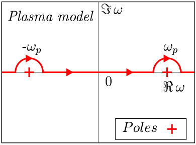
Figure 1: (Color online) The poles of the quantum-mechanical Green functions $G^{\,r}_{p}(\omega)$ (Eq. (55); left panel) and $G^{\,r}_{\text{D}}(\omega)$ (Eqs. (59)–(62); right panel). The parameters $\omega_{\text{pl}},\;\widetilde{\omega}_{\text{pl}}$, and $\gamma$ are specified in Eqs. (54), (62), and (58), respectively. The thick lines with arrows show the paths for integration over $\omega$ in Eqs. (9).

In addition this Green function has a ‘superfluous’ pole at the origin [the first term in the right hand side of (61)] which has no prototype in the Green function $G_{\mathrm{pl}}^{\,r}(\omega)$. In this case the equality (28) works however its application gives contribution to the real part of the Green function $G^{\,r}_{\text{D}}(\omega)$ but not to its imaginary part because of the imaginary coefficient $(-2i\gamma g/\omega_{\text{pl}}^{2})$ in the front of the pole factor $(\omega+i\varepsilon)^{-1}$ in the term under consideration. It is to be noted that this irregular finite contribution emerges for arbitrary, no matter how small, values of the constant $\gamma$. Hence this contribution is non-analytic in $\gamma$ when $\gamma\to 0$. Such an nonanalyticity has been revealed previously in Ref.  [11].

This analysis of analytical properties of the Green function $G^{\,r}_{\text{D}}(\omega)$ shows that the test of the important condition (57) is impracticable in this case.

From all foregoing it follows uniquely that the Green function with the Drude model permittivity, $G_{\mathrm{D}}^{\,r}(\omega)$, cannot be used in the exact AC-relation (34).

However different situation arises in considering the use of $\varepsilon_{\mathrm{D}}(\omega)$ in FDT and consequently in the Lifshitz formula. First of all it is necessary to remind that we finally are interested in the possibility of making use of $\varepsilon_{\mathrm{D}}(\omega)$ for describing the experimental data on the Casimir forces the accuracy of which is about 1%. As it was noted in Sec. IV the accuracy of FDT in the case of dissipative system may be estimated by the extent of dissipative processes, that is by the ratio of the parameter responsible for dissipation to the parameter characterizing reversible part of dynamics. In the Drude model (58) such parameters are respectively $2\gamma$ and $\omega_{\text{pl}}$. In our consideration the typical values of these parameters are provided by gold [36]

$$2\gamma=34{.}5~{}\text{meV},\quad\omega_{\text{pl}}=9{.}03~{}\text{eV}\,{,}$$ (63)

and the aforesaid ratio is

$$\frac{2\gamma}{\omega_{\text{pl}}}=3{.}83\times 10^{-4}\,{.}$$ (64)

This means that the use of $\varepsilon_{\mathrm{D}}(\omega)$ in FDT and, consequently in the Lifshitz formula, is quite admissible from the practical point of view.

Here it is worthy to recall the following peculiarity of the Lifshitz formula. In its final form this formula contains dielectric permittivity $\varepsilon(\omega)$ only along the upper imaginary axis $\omega$, that is, $\varepsilon(i\zeta)$ with real $\zeta$ [27, Chap. VIII, Eq. (81,9)]. As known any physically admissible phenomenological function $\varepsilon(\omega)$ takes on here a real values [37, Chap. IX, §82]. It is this feature of the Lifshitz formula that makes it practically irreplaceable in description of the experimental data on the Casimir forces.

Plasma model and Drude model permittivities, Eqs. (54) and (58), assume real values for pure imaginary $\omega$.

Thus we infer that both permittivities under consideration can be used in the Lifshitz formula practically on the same physical grounds. Therefore it is for comparison with the experiment to decide which permittivity is more suitable to apply in this formula.

It is worthy to note that this inference does not imply that the plasma model and the Drude model permittivities applicable to arbitrary frequencies. The point is these models are based on a simple classical presentation of the electron dynamics in the dielectric or metal materials. In the plasma model electrons are considered to be free. The Drude model, in addition, takes into account the possibility to collide of such electrons with the ions of the crystal lattice. The first model is determined by one dimensional parameter only, plasma frequency $\omega_{\text{pl}}$. The latter model involves, in addition to $\omega_{\text{pl}}$, the free run of the electron that leads to finite conductivity $\sigma$ or damping parameter $\gamma$ (see, for instance, [38, Chap. IV, § 39]).

Therefore it is clear from the physical point of view that the limits of applicability of these two models should be. For example, it is well known that the plasma model permittivity cannot be applicable at low frequencies because it is derived in the limit of high frequencies [37, Chap. IX, §  78]. Theoretically it is reasonable to suggest that the Drude model does not work within some frequency range where it was not independently tested yet.

Besides these two rather simple models it is also interesting to use more complicated models for dielectric permittivity. In Ref. [4] the spatially nonlocal dielectric model is considered which takes dissipation into account and simultaneously agrees with all the measurement data for the Casimir force.

In addition to the Drude model permittivity it is appropriate here to consider briefly the oscillator dielectric permittivity describing isotropic dielectric materials

$$\varepsilon(\omega)=1+\sum_{j=1}^{K}\frac{g_{j}}{\omega_{j}^{2}-\omega^{2}-i\gamma_{j}\omega},$$ (65)

where $g_{j}$ are the oscillator strengths, $\omega_{j}\neq 0$ are the oscillator frequencies, and $\gamma_{j}$ are the dissipation parameters. In this model the dielectric atoms are considered to be weakly damped harmonic oscillators (see, for example, [39], [18, Sec. II]).

The indicated permittivity reduces to the Drude model only in one particular case of the zero oscillator frequency. For all non-zero oscillator frequencies specific for the core electrons in dielectric materials this permittivity describes the narrow resonances with respective small dissipation characteristic for the two-directional exchange of heat in the state of thermal equilibrium (as opposed for the Drude model which possesses the wide resonance at zero oscillator frequency). For this reason, the oscillator dielectric permittivity leads to an agreement between the Lifshitz theory and the measurement data for dielectric materials, on the one hand, and the Nernst heat theorem, on the other hand (see, e.g., F. Chen et al., Ref.  [40]).

Here the following question naturally arises, namely: Is the use of the oscillatory permittivity, Eq. (65), in the Lifshitz formula theoretically grounded, like the use of plasma model and Drude model permittivities? The answer to this question should be positive due to the following reasoning.

This answer can be obtained in the analogous way as it has been done for the Drude model (see Eqs. (63) and (64) above), i.e., we have simply to calculate the expression

$$\sum_{j=1}^{K}\frac{g_{j}\gamma_{j}}{\omega_{j}},\quad j=1,\ldots,K\,{.}$$ (66)

However this numerical calculation is beyond the scope of our study dealing with the plasma model and Drude model permittivities first of all. It is only worthy to note here that, by definition of the oscillator model (65), the pertinent oscillators are considered to be weakly damped [18, Sec. II]. It implies that the sum (66) should be small.

VI Conclusion

In the paper the analysis of theoretical base utilized in derivation of the Lifshitz formula is conducted thoroughly. It is revealed that in different approaches to obtain this formula the use of FDT is an essential step. In view of this a special approach to deriving the FDT is proposed that shows clear in what way the dissipation may be taken into account in this theorem and, consequently, in the Lifshitz formula. Proceeding from this it is shown clear that there are no substantial theoretical arguments in favour of using either plasma mode permittivity or Drude model permittivity in the Lifshitz formula. The decision in this question rests with the comparison of theoretical calculations with the experiment.

In the course of study it is explained how the fluctuation-dissipation theorem works in the case of the system with reversible dynamics, that is when dissipation is absent. Thereby it is proved that explicit assertion according to which this theorem is inapplicable to systems without dissipation is erroneous.

The research is based on making use of the rigorous formalism of equilibrium two-time Green functions in statistical physics at finite temperature and real time. This formalism is grounded on the Hamiltonian approach and hence can be considered as a first principle.

In this connection it is also worth noting the recent works where the dissipation properties in graphene are described on the basis of the first principles of QED at non-zero temperature in the framework of the Dirac model [41]. The respective results were used to calculate the Casimir force in the framework of the Lifshitz theory and found to be in excellent agreement with the measurement data (please see [42, 43]) and with the requirements of thermodynamics [44].

Appendix A Transition to the imaginary frequencies in derivation of the Lifshitz formula with plasma model permittivity at finite temperature

The imaginary frequencies in the Lifshitz formula at finite temperature $T\neq 0$ can be introduced in the same way as it has been done in our work [18] for $T=0$. We explain here the main points of this transition for the plasma model at first.

The Casimir energy at $T=0$ was defined by us as the spectral sum of the zero point energy of electromagnetic field excitations $\hbar\omega/2$:

$$E(2a)=\frac{\hbar}{2}\sum_{\sigma}\int\frac{d^{2}\mathbf{k}}{(2\pi)^{2}}\left[\sum_{n}\omega_{n}(\sigma,k,a)+\int\limits_{\omega_{+}}^{\infty}\omega\Delta\rho(\sigma,\omega,k,a)d\omega\right]-(a\to\infty)\ {.}$$ (67)

This energy is per unite area of the boundaries. In Eq. (67) we use the notations which are generally accepted in the problem in question (see Sec. III of our paper [18]). The first term in square brackets in Eq. (67) is the contribution of the discrete part of the spectrum and the second term represents the contribution of the continuous part of the electromagnetic excitations spectrum in the problem under consideration. In Eq. (67) and further $\sigma=\text{TE,TM}$.

The discrete eigenvalues $\omega_{n}$ in Eq. (67) are the frequencies of the surface modes $\omega_{sm}$ and the waveguide modes $\omega_{wg}$. They are given by the real positive roots of the frequency equations

$$D_{\sigma}(\omega,k,a)\equiv 1-r^{2}_{\sigma}(\omega)e^{4iak_{2}}=0\,{,}$$ (68)

where $r_{\sigma}(\omega)$ is the reflection amplitudes [18]

$$r_{\text{TE}}=\frac{\mu_{2}k_{1}-\mu_{1}k_{2}}{\mu_{2}k_{1}+\mu_{1}k_{2}},\quad r_{\text{TM}}=\frac{\varepsilon_{2}k_{1}-\varepsilon_{1}k_{2}}{\varepsilon_{2}k_{1}+\varepsilon_{1}k_{2}}\,{.}$$ (69)

Just as in Ref. [18], we assume that $\varepsilon_{2}=\mu_{1}=\mu_{2}=1$ and the permittivity $\varepsilon_{1}(\omega)$ is defined in Eq. (54). The wave vectors $k_{1}$ and $k_{2}$ are specified below.

The spectral density shift in Eq. (67), $\Delta\rho(\omega)$, as the function of the real frequency $\omega$, is given by a known expression

$$\Delta\rho(\omega)=\frac{1}{\pi}\,\frac{d}{d\omega}\delta(\omega)\,{,}$$ (70)

where $\delta(\omega)$ is the phase shift. Thus Eq. (67) involves only real positive frequencies $\omega$.

In order to pass to imaginary frequencies the outcome to complex plane $\omega$ is needed. For this aim in Ref. [18] two cuts have been made on this plane, namely, the first cut between the points $-\omega_{-}(k)$ and $\omega_{-}(k)$ and the second one on the interval $(\omega_{+}(k),\infty)$ [see Fig. 2]. The points $\omega_{-}(k)$ and $\omega_{+}(k)$ are the branch points of the functions

$$ck_{1}(\omega)=\sqrt{\omega^{2}-\omega_{+}^{2}(k)},\quad ck_{2}(\omega)=\sqrt{\omega^{2}-\omega_{-}^{2}(k)},$$ (71)

$$\omega_{+}^{2}(k)=\omega_{\mathrm{pl}}^{2}+c^{2}k^{2},\quad\omega_{-}^{2}(k)=c^{2}k^{2},$$ (72)

and, at the same time, they determine the boundaries between the different branches of the spectrum, namely, on the interval $0<\omega_{sm}(k)<\omega_{-}(k)$ the surface mode frequencies are located, on the interval $\omega_{-}(k)<\omega_{wg}(k)<\omega_{+}(k)$ the waveguide mode frequencies lie, and the interval $\omega_{+}(k)<\omega(k)<\infty$ belongs to the continuous spectrum.

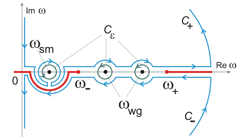
Figure 2: (Color online) The contours $C_{+}$ and $C_{-}$ in the complex $\omega$ plane which are used when going on to the imaginary frequencies. For simplicity, the spectrum possessing one surface mode $\omega_{\text{\,sm}}$, two waveguide modes $\omega_{\text{\,wg}}$, and the continuous part $\omega>\omega_{+}$ is considered. The cuts starting at the points $\omega_{-}$ and $\omega_{+}$ are shown by thick lines.

The single-valued branches of the functions (71) are extracted by the requirements that the function $k_{2}(\omega)$ takes on real positive values on the upper edge of the cut $(\omega_{+}(k),\infty)$, and the values of the function $k_{1}(\omega)$ on the upper edge of the cut $(-\omega_{-}(k),\omega_{-}(k))$ have the argument $\pi/2$. Taking account of this one can easily be convinced that the functions $D_{\sigma}(\omega)$ and $\overline{D_{\sigma}(\omega)}$ acquire the same values in the interval $(\omega_{-}(k),\omega_{+}(k))$ of the real axis and at the opposite points lying on the different edges of the cut $(0,\omega_{-}(k))$.

Further we shall need the properties of the frequency equation (68), that is of the function $D_{\sigma}(\omega)$, in the upper half-plane $\Omega$ of the complex variable $\omega$. The plasma model permittivity (54) is considered.

1. The function $D_{\sigma}(\omega)$ tends to $1$ for $|\omega|\to\infty,\;\omega\in\Omega$.

2. $D_{\sigma}(\omega)=D_{\sigma}(-\omega)$ see Eqs. (68), (69), (71), (72), and (54).

3. Along the imaginary positive semi-axis the function $D_{\sigma}(\omega)$ assumes real values.

4. Equation (68) has no complex roots in $\Omega$, that is the frequencies of the quasi-normal modes, if they exist, have negative imaginary part. Otherwise the macroscopic electrodynamics would admit the natural modes increasing in time without limits. Recall that the time dependence is taken, as usual, in the form $e^{-i\omega t}$. These properties of the quasi-normal modes are explicitly ascertained for electromagnetic oscillations of a perfectly conducting sphere [47] and a dielectric ball without dispersion [48, 49, 50].

5. As follows from Eq. (68), the poles of the function $D_{\sigma}(\omega)$ may be generated only by the reflection amplitude, $r_{\sigma}(\omega)$, and their position on the complex $\omega$-plane is independent of the gap width $2a$. Therefore the contribution of these poles to the vacuum energy (67) will be canceled when subtracting in this formula the respective limiting expression obtained for $a\to\infty$. Hence these poles can be disregarded.

6. The function $\overline{D_{\sigma}(\omega)}$ possesses the same properties in $\overline{\Omega}$ .

Employing the argument principle theorem (see Sec. 3.4 of Ref. [51]) we represent the contribution of the discrete spectrum into (67) in the following form

$$\omega_{n}=\frac{1}{2\pi i}\oint_{C_{\varepsilon}}d\omega\,\omega\frac{d}{d\omega}\ln D_{\sigma}(\omega)\,{,}$$ (73)

where $C_{\varepsilon}$ is a circle of the radius $\varepsilon$ with $\varepsilon\to 0$, see Fig. 2. The spectral density shift $\Delta\rho$, as the function of the complex variable $\omega$, is defined ultimately by the function $D_{\sigma}(\omega)$

$$\Delta\rho(\omega)=\frac{1}{2\pi i}\,\frac{d}{d\omega}\ln\frac{\overline{D_{\sigma}(\omega+i0)}}{D_{\sigma}(\omega+i0)}$$ (74)

(see details in Ref. [18]). In Eq. (74) we explicitly note that the function $D(\omega+i0)$ is calculated at the upper edge of the cut $(\omega_{+},\infty)$ and the function $\overline{D(\omega+i0)}$ is calculated at the lower edge of this cut.

Taking into account Eqs. (73) and (74), we can now represent the vacuum energy (67) in the following form

$$E(2a)=\frac{\hbar}{2}\sum_{\sigma}\int_{0}^{\infty}\frac{kdk}{2\pi}\frac{1}{2\pi i}\left[\sum_{C_{\varepsilon}}\oint_{C_{\varepsilon}}d\omega\,\omega\frac{d}{d\omega}\ln D_{\sigma}(\omega)+\int_{\omega_{+}}^{\infty}d\omega\,\omega\frac{d}{d\omega}\ln\frac{\overline{D_{\sigma}(\omega+i0)}}{D_{\sigma}(\omega+i0)}\right]\!.$$ (75)

The properties of the functions $D_{\sigma}(\omega)$ and $\overline{D_{\sigma}(\omega)}$ enumerated above enable us to write the following equalities

$$\frac{1}{2\pi i}\oint_{C_{+}}\omega\frac{d}{d\omega}\ln D_{\sigma}(\omega)d\omega=0\,{,}$$ (76)

$$\frac{1}{2\pi i}\oint_{C_{-}}\omega\frac{d}{d\omega}\ln\overline{D_{\sigma}(\omega)}d\omega=0\,{,}$$ (77)

where the contours $C_{+}$ and $C_{-}$ enclose, respectively, the first and the fourth quadrants of the $\omega$-plane as depicted in Fig. 2.

Further we proceed in the following way: the integral in Eq. (75), containing the function $D_{\sigma}(\omega+i0)$ on the upper edge of the cut $(\omega_{+},\infty)$, we express from Eq. (76) and the integral including the function $\overline{D_{\sigma}(\omega+i0)}$, evaluated on the lower edge of this cut, we express from Eq. (77). Doing in this way we can disregard, in virtue of the property i), the contributions due to the arcs of the big circle. One can easily see from Fig. 2 that along the contours $C_{\varepsilon}$ the contributions of the discrete spectrum and the continuous spectrum are mutually canceled. In addition, the integrals with the function $D_{\sigma}(\omega+i0)$ and $\overline{D_{\sigma}(\omega+i0)}$ between the origin and the point $\omega_{+}$ are reciprocally canceled too. As the result the integration only along the imaginary axis ($\omega=i\zeta$) survives:

$$E(2a)=-\frac{\hbar}{2}\sum\limits_{\sigma}\int_{0}^{\infty}\frac{kdk}{(2\pi)^{2}}\left[\int_{0}^{\infty}d\zeta\,\zeta\frac{d}{d\zeta}\ln D_{\sigma}(i\zeta,k)+\int_{-\infty}^{0}d\zeta\,\zeta\frac{d}{d\zeta}\ln\overline{D_{\sigma}(i\zeta,k)}\right]\!{.}$$ (78)

Taking into account the property iii), we can join two integrals in Eq. (78) in one integral with the limits $(-\infty,\infty)$ and after that we accomplish the integration by parts. The terms outside the integral vanish in view of the property i). As a result Eq. (78) acquires the form

$$E(2a)=\frac{\hbar}{2}\sum_{\sigma}\int_{0}^{\infty}\frac{k\,dk}{(2\pi)^{2}}\int_{-\infty}^{\infty}d\zeta\,\ln D_{\sigma}(i\zeta,k)=\frac{\hbar}{2\pi}\sum_{\sigma}\int_{0}^{\infty}\frac{k\,dk}{2\pi}\int_{0}^{\infty}d\zeta\,\ln D_{\sigma}(i\zeta,k)$$ (79)

(see Eqs. (71) and (72) in our paper [18]). The last equality in Eq. (79) is obtained on account of the property ii).

Differentiation of the vacuum energy (79) with respect to the gap width $2a$ results in the standard representation of the Lifshitz formula at zero temperature (see Eqs. (73) and (75) in Ref. [18]).

We shall not write out these well known formulas but at once go over to derivation of the Lifshitz formula at finite temperature $T$. To this end the free energy $\mathcal{F}$ of electromagnetic field in the problem at hand should be found. We accomplish this task by summing up, with respect to the spectrum of electromagnetic excitations, the free energy of quantum oscillator

$$f(\omega)=\frac{\hbar\omega}{2}+k_{\text{B}}T\ln\left[1-\exp\left(-\frac{\hbar\omega}{k_{\text{B}}T}\right)\right]\!{,}$$ (80)

where $k_{\text{B}}$ is the Boltzman constant. Thus in all formulas beginning with Eq. (67), the zero point energy $\hbar\omega/2$ should be replaced by $f(\omega)$. The function $f(\omega)$ has logarithmic branch points for $\omega=i\zeta_{m}$, where $\zeta_{m}$ are the Matsubara frequencies

$$\zeta_{m}=2\pi mk_{\text{B}}T/\hbar,\quad m=0,\pm 1,\pm 2,\ldots\,{.}$$ (81)

The introduction of respective cuts in the $\omega$-plane can be avoided by using formal and nevertheless rather rigorous method [52, 53], namely, the function $f(\omega)$ in Eq. (80) should be represented by the series

$$f(\omega)=\frac{\hbar\omega}{2}-k_{\text{B}}T\sum_{m=1}^{\infty}\frac{1}{m}\exp\left(-\frac{m\hbar\omega}{k_{\text{B}}T}\right)\!{.}$$ (82)

It is easy to see that after substitution of $\hbar\omega/2$ for $f(\omega)$ in Eq. (78) the expression

$$\frac{f(i\zeta)}{i}\equiv\varphi(\zeta)=\frac{\hbar\zeta}{2}+ik_{\text{B}}T\sum_{m=1}^{\infty}\frac{1}{m}\exp\left(-i\frac{m\hbar\zeta}{k_{\text{B}}T}\right){.}$$ (83)

will be here in place of $\zeta$. In this notation Eq. (78) assumes the form

$$\mathcal{F}(2a)=-\sum_{\sigma}\int_{0}^{\infty}\frac{kdk}{(2\pi)^{2}}\left[\int_{0}^{\infty}d\zeta\varphi(\zeta)\frac{d}{d\zeta}\ln D_{\sigma}(i\zeta,k)+\int_{-\infty}^{0}d\zeta\varphi(\zeta)\frac{d}{d\zeta}\ln\overline{D_{\sigma}(i\zeta,k)}\right]\!{.}$$ (84)

Taking into account the property iii), we can again join two integrals in Eq. (84) into one

$$\mathcal{F}(2a)=-\sum_{\sigma}\int_{0}^{\infty}\frac{kdk}{(2\pi)^{2}}\int_{-\infty}^{\infty}d\zeta\,\varphi(\zeta)\frac{d}{d\zeta}\ln D_{\sigma}(i\zeta,k)\,{.}$$ (85)

The integration by parts with allowance for the property i) gives

$$\mathcal{F}(2a)=\sum_{\sigma}\int_{0}^{\infty}\frac{kdk}{(2\pi)^{2}}\int_{-\infty}^{\infty}d\zeta\,\varphi^{\prime}(\zeta)\ln D_{\sigma}(i\zeta,k)$$

$$=\hbar\sum_{\sigma}\int_{0}^{\infty}\frac{kdk}{(2\pi)^{2}}\int_{-\infty}^{\infty}d\zeta\left[\frac{1}{2}+\sum_{m=1}^{\infty}\exp\left(-im\hbar\zeta{k_{\text{B}}T}\right)\right]\ln D_{\sigma}(i\zeta,k)$$

$$=\hbar\sum_{\sigma}\int_{0}^{\infty}\frac{kdk}{(2\pi)^{2}}\int_{-\infty}^{\infty}d\zeta\left[\left(\frac{1}{2}+\sum_{m=1}^{\infty}\cos m\hbar\zeta{k_{\text{B}}T}\right)-i\sum_{m=1}^{\infty}\sin m\hbar\zeta{k_{\text{B}}T}\right]\ln D_{\sigma}(i\zeta,k)\,{.}$$ (86)

By virtue of the property ii) the second sum over $m$ in Eq. (86) does not contribute to the integral over $d\zeta$. Now we take advantage of the Fourier series representation for the “comb” of $\delta$-functions

$$\pi k_{\text{B}}T\sum_{m=-\infty}^{\infty}\delta(\zeta-2\pi mk_{\text{B}}T/\hbar)=\hbar\left(\frac{1}{2}+\sum_{m=1}^{\infty}\cos m\hbar\zeta{k_{\text{B}}T}\right)\!{.}$$ (87)

The substitution of (87) into (86) replaces the integration over $d\zeta$ by the summation over the Matsubara frequencies (81)

$$\mathcal{F}(2a) =\pi k_{\text{B}}T\sum_{\sigma}\int_{0}^{\infty}\frac{k\,dk}{(2\pi)^{2}}\sum_{m=-\infty}^{\infty}\ln D_{\sigma}(i\zeta_{m},k)$$

$$=k_{\text{B}}T\sum_{\sigma}\int_{0}^{\infty}\frac{k\,dk}{2\pi}\mathop{{\sum}^{\prime}}_{m=0}^{\infty}\ln D_{\sigma}(i\zeta_{m},k)\,{.}$$ (88)

The primed sign of the sum implies that the term with $m=0$ should be multiplied by $1/2$. The last expression in (88) is obtained owing to the property ii). The free energy (88) coincides exactly with Eq. (12.66) in the book [1].

Differentiation of Eq. (88) with respect to the width of the gap $2a$, gives at once the Lifshitz formula for the Casimir force at nonzero temperature (see Eq. (12.70) in Ref. [1]).

The change of the integration variable $k$ in Eq. (88)

$$k^{2}=\frac{\zeta_{m}^{2}}{c^{2}}(p^{2}-1),\quad k\,dk=\frac{\zeta_{m}}{c^{2}}p\,dp,\quad 1<p<\infty$$ (89)

enables one to reproduce the Lifshitz formula in the original form (see Eq. (81.9) in Ref. [27] for two identical material semi-spaces separated by a vacuum gap).

The transition to the Matsubara frequencies in deriving the Lifshitz formula, presented above, substantially relied on using the properties i)–vi) of the functions $D_{\sigma}(\omega,k,a)$ in the frequency equations (68).

- [1] M. Bordag, G. L. Klimchitskaya, U. Mohideen, and V. M. Mostepanenko, Advances in the Casimir Effect (Oxford University Press, Oxford, 2009).
- [2] K. A. Milton, The Casimir Effect: Physical Manifestations of Zero-Point Energy, (World Scientific, Singapore, 2001).
- [3] M. Bordag, I. Fialkovsky, N. Khusnutdinov, and D. Vassilevich, Phys. Rev. B 104, 195431 (2021).
- [4] G. L. Klimchitskaya, V. M. Mostepanenko, Phys. Rev. A 105, 012805 (2022).
- [5] V. B. Bezerra, R. S. Decca, E. Fischbach, B. Geyer, G. L. Klimchitskaya, D. E. Krause, D. Lopez, V. M. Mostepanenko, and C. Romero, Phys. Rev. E 73, 028101 (2006).
- [6] R. S. Decca, D. Lopez, E. Fischbach, G. L. Klimchitskaya, D. E. Krause, V. M. Mostepanenko, Ann. Phys. (N.Y.) 318, 37 (2005).
- [7] J. S. Høye, I. Brevik, J. B. Aarseth, and K. A. Milton, J. Phys. A: Math. Gen. 39, 6031 (2006).
- [8] R. Guérout, A. Lambrecht, K. A. Milton, and S. Reynaud, Phys. Rev. E 90, 042125 (2014).
- [9] J. S. Høye, I. Brevik, Phys. Rev. A 93, 052504 (2016).
- [10] M. Bordag, I. G. Pirozhenko, Phys. Rev. D 82, 125016 (2010).
- [11] M. Bordag, Eur. Phys. J. C 71, 1788 (2011).
- [12] E. M. Lifshitz, Zh. Eksp. Teor. Fiz. 29, 94 (1955) [Sov. Phys. JETP 2, 73 (1956)].
- [13] L. L. Landau and E. M. Lifshitz, Electrodynamics of Continuous Media (Pergamon Press, Oxford, 1960), pp. 368–376.
- [14] H. B. Callen and T. A. Welton, Phys. Rev. 83, 34 (1951).
- [15] R. Kubo, J. Phys. Soc. Japan 12, 570 (1957).
- [16] R. Kubo, Rep. Prog. Phys. 29, 255 (1966).
- [17] L. D. Landau and E. M. Lifshitz, Statistical Physics, Part 1 (Pergamon Press, Oxford, 1980), Chap. XII.
- [18] V. V. Nesterenko, I. G. Pirozhenko, Phys. Rev. A 86, 052503 (2012); arXiv:1112.2599v2 [quant-ph].
- [19] H. B. G. Casimir, Proc. Kon. Ned. Akad. Wet. 51, 793 (1948).
- [20] S. M. Rytov, Theory of Electric Fluctuations and Thermal Radiation (Academy of Sciences of USSR, Moscow, 1953) [in Russian]; Engl. transl.: U.S. Air Cambridge Research Center (Bedford, Massachusetts) Report No. AFCRC-TR-59-162, 1959 (unpublished).
- [21] S. M. Rytov, Y. A. Kravtsov, and V. I. Tatarskii, Principles of Statistical Radiophysics, Vol. 3: Elements of Random Fields (Springer, Berlin, 1989).
- [22] M. L. Levin, S. M. Rytov, Theory of Equilibrium Thermal Fluctuations in Electrodynamics (Nauka, Moscow, 1967) [in Russian].
- [23] W. Eckhardt, Phys. Rev. A 29, 1991 (1984).
- [24] D. Polder and M. Van Hove, Phys. Rev. B 4, 3303 (1971).
- [25] G. S. Agarval, Phys. Rev. A 11, 230; 243 (1975).
- [26] I. E. Dzyaloshinskii, E. M. Lifshitz, and L. P. Pitaevskii, Adv. Phys. 10, 165 (1961).
- [27] E. M. Lifshitz and L. P. Pitaevskii, Statistical Physics, Part 2 (Pergamon Press, Oxford, 1980), Chap. VIII.
- [28] A. A. Abrikosov, L. P. Gor’kov, and I. Ye. Dzyaloshinsckii, Quantum Field Theoretical Methods in Statistical Physics (Pergamon, New York, 1965).
- [29] D. N. Zubarev, Usp. Fiz. Nauk 71, 71 (1960) [Sov. Phys. Usp. 3, 320 (1960)].
- [30] D. N. Zubarev, Nonequilibrium Statistical Thermodynamics (Consultant Bureau, New York, 1974).
- [31] N. N. Bogoliubov, D. V. Shirkov, Introduction to the Theory of Quantized Field, 3rd ed. (Wiley, 1980).
- [32] K. Blum, Density Matrix Theory and Applications, Springer Series on Atomic, Optical, and Plasma Physics, Vol. 64, 3rd ed. (Springer, 2012).
- [33] V. L. Ginzburg, Usp. Fiz. Nauk 46, 348 (1952); 52, 494 (1954); V. I. Tatarskii, ibid. 151, 273 (1987) [Sov. Phys. Usp. 30, 134 (1987)]; Yu. L. Klimontovich, ibid. 151, 309 (1987) [Sov. Phys. Usp. 30, 154 (1987)]; V. L. Ginzburg and L. P. Pitaevzkii, ibid. 151, 333 (1987) [Sov. Phys. Usp. 30, 168 (1987)]; N. G. Van Kampen, Physica Norvegica 5, 279 (1971)]; K. M. Van Vliet, J. Math. Phys. 20, 2573 (1979); M. Charbonneau, K. M. van Vliet, and P. Vasilopoulos, ibid. 23, 318 (1982); P. Vasilopoulos, Carolyn M. Van Vliet, ibid. 25, 1391 (1984); Carolyn M. Van Vliet, J. Stat. Phys. 53, 50 (1988).
- [34] D. N. Zubarev, Yu. G. Rudoi, Usp. Fiz. Nauk 163, No. 3, 103 (1993) [Phys. Usp. 36, No. 3, 188 (1993)].
- [35] I. Brevik, B. Shapiro, J. Phys. Commun. 6, 015005 (2022).
- [36] J. S. Høye, I. Brevik, S. A. Ellingsen, and J. B. Aarseth, Phys. Rev. E 75, 051127 (2007).
- [37] L. D. Landau, E. M. Lifshitz, and L. P. Pitaevskii, Electrodynamics of Continuous Media (Pergamon Press, Oxford, 1984).
- [38] A. Sommerfeld, Thermodynamik und Statistik, Wiesbaden, 1952, Kap. IV, § 35.
- [39] M. Born and E. Wolf, Principles of Optics, 6th ed. (Pergamon, New York, 1941).
- [40] F. Chen, G. L. Klimchitskaya, V. M. Mostepanenko, and U. Mohideen, Phys. Rev. B 76, 035338 (2007).
- [41] M. Bordag, I. V. Fialkovsky, D. M. Gitman, and D. V. Vassilevich, Phys. Rev. B 80, 245406 (2009).
- [42] M. Liu, Y. Zhang, G. L. Klimchitskaya, V. M. Mostepanenko, and U. Mohideen, Phys. Rev. Lett. 126, 206802 (2021).
- [43] M. Liu, Y. Zhang, G. L. Klimchitskaya, V. M. Mostepanenko, and U. Mohideen, Phys. Rev. B 104, 085436 (2021).
- [44] G. L. Klimchitskaya and V. M. Mostepanenko, Phys. Rev. D 102, 016006 (2020).
- [45] P. Debye, Annalen der Physik 338, 1427 (1910).
- [46] M. Planck, Theorie der Wärme, der Einführung in die teoretische Physik, Band V, 4 Auflage (Leipzig, 1921).
- [47] V. V. Nesterenko, J. Phys. A: Math. Theor. 41, 164005 (2008).
- [48] P. Debye, Ann. Phys. (Leipzig) 30, 57 (1909); G. Mie, ibid. 25, 377 (1908).
- [49] M. Gastine, L. Courtois, J. L. Dormann, IEEE Trans. Microwave Theory and Techniques 15, 694 (1967).
- [50] V. V. Nesterenko, A. Feoli, G. Lambiase, and G. Scarpetta, Mod. Phys. Lett. B 22, 735 (2008); arXiv: hep-th/0512340.
- [51] E. C. Titchmarsh, The theory of functions (Oxford University Press, London, 1939).
- [52] V. V. Nesterenko, I. G. Pirozhenko, J. Math. Phys. 38, 6265 (1997).
- [53] B. W. Ninham, V. A. Parsegian, and G. H. Weiss, J. Stat. Phys. 2, 323 (1970).
- [54] G. A. Korn, T. M. Korn, Mathematical Handbook, 2nd ed. (McGraw-Hill, New York, 1968).