1 Introduction

The Standard Model (SM) of particle physics successfully describes the fundamental interactions of the known matter fields at the present level of experimental accuracy. In particular, the discovery of a scalar particle with a mass of $\approx 125\ \mathrm{GeV}$ at the Large Hadron Collider (LHC) [1, 2], that within the current experimental uncertainties [3, 4, 5] behaves as predicted by the realisation of the Brout-Englert-Higgs mechanism within the SM [6, 7], has confirmed the existence of a non trivial vacuum structure of the universe. Despite the great success of the SM, there are also phenomena that cannot be accommodated, and furthermore the SM has conceptual shortcomings. In particular, the SM does not provide a sizable contribution to the relic abundance of cold dark matter, the neutrino oscillation data cannot be explained with strictly massless SM neutrinos, there is no mechanism to account for the observed matter-antimatter asymmetry of the universe, and there is no consistent formulation of the SM that includes gravitational interactions.

Another conceptual problem of the SM is related to the fact that its scalar sector, incorporating a single SU(2) doublet scalar field, just provides a minimal parameterization of electroweak symmetry breaking. The renormalizable scalar potential of the SM can be expressed in terms of only two parameters, e.g., the vacuum expectation value (vev), $v\approx 246\ \mathrm{GeV}$, and the mass of the predicted Higgs boson, which within the SM is identified with the mass of the detected particle, $m_{h_{125}}\approx 125\ \mathrm{GeV}$. This minimal construction is sufficient to generate the masses of the gauge bosons, the Higgs boson, the quarks and the charged leptons via spontaneous symmetry breaking. However, within the SM there is no dynamical origin of the Higgs potential, and the mass of the Higgs boson of the SM is not protected by symmetries against large corrections from physics at high scales. This gives rise to the so-called hierarchy problem [8, 9] regarding the observed value of $m_{h_{125}}$ and more generally the stability of the electroweak (EW) scale.

One of the most thoroughly studied frameworks of BSM physics is Supersymmetry (SUSY). Models based on SUSY provide a solution for the hierarchy problem, since the symmetry between bosonic and fermionic degrees of freedom leads to a cancellation between contributions with a quadratic dependence on new physics at higher energies [10, 11, 12], thus protecting the masses of the Higgs bosons of the model. Furthermore, for the observed gauge bosons and the states in the Higgs sector SUSY predicts new fermionic superpartners, as well as new bosonic superpartners for the three generations of quarks and leptons. As a result, SUSY extensions of the SM have a substantially richer matter sector, and in addition to the hierarchy problem many other shortcomings of the SM can be addressed as well. For instance, there are several possible candidates for cold dark matter.

A particularly well motivated SUSY model is the $\mu$-from-$\nu$ Supersymmetric Standard Model ($\mu\nu$SSM) [13, 14]. Beyond the well-known appealing features of commonly studied SUSY models, in the $\mu\nu$SSM the tiny neutrino masses and their mixings can be accommodated via an EW seesaw mechanism, where it is required that the matter content is enlarged w.r.t. the SM by right-handed neutrinos [16, 17, 18, 19, 20]. Their superpartners, the “right-handed” scalar neutrinos (sneutrinos), are gauge singlet scalar fields. If the right-handed sneutrinos acquire vevs, the so-called $\mu$-term of the Minimal Supersymmetric Standard Model (MSSM) can be generated effectively, in complete analogy to the $Z_{3}$ symmetric Next-to-MSSM (NMSSM). Consequently, the $\mu\nu$SSM also provides a solution to the so-called $\mu$-problem [21, 22]. By construction, the $\mu\nu$SSM does not allow for a consistent assignment of conserved $R$ parity charges, giving rise to the fact that there is no stable lightest SUSY particle. Compared to the (N)MSSM, the collider constraints from the LHC are therefore substantially weaker [23, 24, 25, 26, 27, 28]. Regarding dark matter, it is possible to accommodate the measured relic abundance by means of decaying, but long-lived, gravitinos or axinos [29, 30, 31].

One of the key features of the $\mu\nu$SSM is the mixing of the two Higgs doublet fields $H_{d}$ and $H_{u}$ with the three left-handed and right-handed sneutrino fields $\widetilde{\nu}_{iL}$ and $\widetilde{\nu}_{iR}$, leading to a total of eight neutral CP-even particles and seven neutral CP-odd scalar particles. While the mixing of the left-handed sneutrinos with the Higgs doublet fields is suppressed by the smallness of lepton number breaking, the mixing of the right-handed sneutrinos with the Higgs fields can be sizable, while being in agreement with the current experimental limits [27, 32]. The phenomenological consequences of the latter possibility have been thoroughly studied, paying special attention to the prediction for the mass of the SM-like Higgs boson [33, 32, 34]. In addition to the more complicated scalar particle spectrum, the enlarged Higgs sector compared to the SM and the (N)MSSM also results in a substantially more complicated scalar potential. While it is always possible to ensure the existence of a phenomenologically viable EW vacuum by conveniently choosing the vevs of the neutral scalar fields as input parameters (as will be discussed in Sect. 2), the scalar potential of the $\mu\nu$SSM in general contains further unphysical local minima. If one or more of the unphysical minima are deeper than the EW minimum, the question arises whether the EW vacuum can become short-lived in comparison to the age of the universe, and if this is the case the corresponding parameter point should be rejected.

Up to now no detailed analysis of constraints on the parameter space of the $\mu\nu$SSM arising from possible instabilities of the EW vacuum has been carried out in the literature. To the best of our knowledge, only Ref. [16] took into account such constraints, demanding, however, that the EW minimum is the global minimum of the potential, i.e. the possibility of a long-lived metastable EW vacuum was not taken into account. Apart from that, heuristic constraints that have been obtained for the presence of color-breaking unphysical minima in the MSSM could be considered [35]. Besides their limited reliability, constraints of this kind do not capture the possibility that charge- and color-conserving minima can nevertheless be unphysical. Accordingly, we study in this paper the impact of genuine effects of the $\mu\nu$SSM on the stability of the EW vacuum.

In this paper, we perform a detailed analysis of the neutral scalar potential of the $\mu\nu$SSM regarding EW vacuum instabilities. In a first step, we determine the unphysical minima of the tree-level neutral scalar potential by making use of an homotopy continuation method. In a second step, we estimate the rates for the decays of the EW vacuum into all unphysical minima below the EW minimum using a semi-classical approximation. By subsequently comparing these rates to the age of the universe, we categorize parameter points into ones with a short-lived (unstable), long-lived (metastable) and an absolutely stable EW vacuum, and we discuss the impact of the resulting constraints on the parameter space of the model. As an example scenario, in our numerical analysis we apply the investigation of vacuum stability constraints to the alignment-without-decoupling limit of the $\mu\nu$SSM. It turns out that in this limit the EW minimum is not the global minimum of the potential. However, in large parts of the analyzed parameter regions the decay rates into the unphysical minima are so small that the EW vacuum is long-lived compared to the age of the universe, and those parameter regions with a metastable vacuum are therefore phenomenologically viable.

The paper is organized as follows: In Sect. 2 we introduce the Higgs sector of the $\mu\nu$SSM, followed by a discussion of the alignment without decoupling limit in Sect. 3. In Sect. 4 we describe the determination of the minima of the neutral scalar potential and the procedure that is applied for assessing the stability of the EW vacuum. In Sect. 5 we apply this approach to example scenarios in the alignment limit. Finally, we summarize our results and give a brief outlook on possible avenues for future research in Sect. 6. In the appendix we briefly describe the public code munuSSM that can be used for performing the vacuum stability test in the $\mu\nu$SSM parameter space. We furthermore provide explicit expressions for the coefficients of the scalar potential relative to the EW vacuum for some special cases.

2 The neutral scalar sector of the $\mu\nu$SSM

The neutral scalar potential of the $\mu\nu$SSM consists of contributions from the superpotential $W$ and the soft SUSY-breaking Lagrangian $\mathcal{L}_{\rm soft}$. The part of $W$ that contains the neutral superfields is given by [13, 14]

$$W=\; \epsilon_{ab}\left(Y^{\nu}_{ij}\,\hat{H}_{u}^{b}\,\hat{L}^{a}_{i}\,\hat{\nu}^{c}_{j}-\lambda_{i}\,\hat{\nu}^{c}_{i}\,\hat{H}_{u}^{b}\hat{H}_{d}^{a}\right)+\frac{1}{3}\kappa{{}_{ijk}}\hat{\nu}^{c}_{i}\hat{\nu}^{c}_{j}\hat{\nu}^{c}_{k}+\dots\ ,$$ (1)

where $\hat{H}_{d}^{T}=(\hat{H}_{d}^{0},\hat{H}_{d}^{-})$ and $\hat{H}_{u}^{T}=(\hat{H}_{u}^{+},\hat{H}_{u}^{0})$ are the Higgs doublet superfields, $\hat{L}_{i}$ are the left-chiral lepton superfields with the left-chiral neutrino superfields $\hat{\nu}_{i}$ in the upper component, and $\hat{\nu}^{c}$ are the right-chiral neutrino superfields. ${i,j=1,2,3}$ are the family indices, and ${a,b=1,2}$ are the weak isospin indices $(\epsilon_{12}=1)$. The portal couplings $\lambda_{i}$ give rise to the mixing between the right-handed sneutrinos and the Higgs doublet fields, and also the $\mu$-term is generated after electroweak symmetry breaking (EWSB) ($\mu=\lambda_{i}v_{iR}/\sqrt{2}$). The self-couplings $\kappa_{ijk}$ generate masses for the right-handed (s)neutrinos after EWSB, such that they determine the scale of the seesaw mechanism. Since the seesaw scale is in this way related to the EW scale, for the neutrino Yukawa couplings one has to demand $Y^{\nu}_{ij}\lesssim Y_{e}\approx 10^{-6}$, with $Y_{e}$ the electron Yukawa coupling, in order to obtain left-handed neutrino masses at the sub-eV level.

The part of $\mathcal{L}_{\rm soft}$ that contains the neutral scalar fields can be written as [13, 14]

$$-\mathcal{L}_{\text{soft}} =\epsilon_{ab}\left(T^{\nu}_{ij}\,H_{u}^{b}\,\widetilde{L}^{a}_{iL}\widetilde{\nu}_{jR}^{*}-T^{\lambda}_{i}\,\widetilde{\nu}_{iR}^{*}\,H_{d}^{a}H_{u}^{b}+\frac{1}{3}T^{\kappa}_{ijk}\,\widetilde{\nu}_{iR}^{*}\widetilde{\nu}_{jR}^{*}\widetilde{\nu}_{kR}^{*}\ +\text{h.c.}\right)$$

$$+\ \left(m_{\widetilde{L}}^{2}\right)_{ij}\widetilde{L}_{iL}^{a*}\widetilde{L}^{a}_{jL}+\left(m_{\widetilde{\nu}}^{2}\right)_{ij}\widetilde{\nu}_{iR}^{*}\widetilde{\nu}_{jR}+m_{H_{d}}^{2}{H^{a}_{d}}^{*}H^{a}_{d}+m_{H_{u}}^{2}{H^{a}_{u}}^{*}H^{a}_{u}+\dots\ ,$$ (2)

where $H_{d}$, $H_{u}$, $\widetilde{\nu}_{iL}$ and $\widetilde{\nu}_{iR}$ denote the scalar components of the superfields $\hat{H}_{d}$, $\hat{H}_{u}$, $\hat{\nu}_{i}$ and $\hat{\nu}_{i}^{c}$, respectively. As usual, soft mass parameters that are non-diagonal in field space are neglected. Thus, terms of the form $((m_{H_{d}\widetilde{L}}^{2})_{i}H_{d}^{a*}\widetilde{L}_{iL}^{a}+\mathrm{h.c.})$ are absent, and the matrices $m_{\widetilde{L}}^{2}$ and $m_{\widetilde{\nu}}^{2}$ are assumed to be diagonal. For the trilinear scalar couplings, we will make use of the decomposition $T^{\nu}_{ij}=A^{\nu}_{ij}Y^{\nu}_{ij}$, $T^{\lambda}_{i}=A^{\lambda}_{i}\lambda_{i}$, $T^{\kappa}_{ijk}=A^{\kappa}_{ijk}\kappa_{ijk}$, which is motivated in models of supergravity with diagonal Kähler metric [36].

The soft terms shown above, in combination with the $D$- and $F$-terms derived from the superpotential, give rise to the neutral scalar potential

$$V=V_{\text{soft}}+V_{F} +V_{D}\ ,\;\text{with}$$ (3)

$$V_{\text{soft}}=\; \left(T^{\nu}_{ij}\,H_{u}^{0}\,\widetilde{\nu}_{iL}\,\widetilde{\nu}_{jR}^{*}-T^{\lambda}_{i}\,\widetilde{\nu}_{iR}^{*}\,H_{d}^{0}H_{u}^{0}+\frac{1}{3}T^{\kappa}_{ijk}\,\widetilde{\nu}_{iR}^{*}\widetilde{\nu}_{jR}^{*}\widetilde{\nu}_{kR}^{*}\ +\text{h.c.}\right)$$

$$+\; \left(m_{\widetilde{L}}^{2}\right)_{ij}\widetilde{\nu}_{iL}^{*}\widetilde{\nu}_{jL}+\left(m_{\widetilde{\nu}}^{2}\right)_{ij}\widetilde{\nu}_{iR}^{*}\widetilde{\nu}_{jR}+m_{H_{d}}^{2}{H^{0}_{d}}^{*}H^{0}_{d}+m_{H_{u}}^{2}{H^{0}_{u}}^{*}H^{0}_{u}\ ,$$ (4)

$$V_{F}=\; \lambda_{j}\lambda_{j}H^{0}_{d}H_{d}^{0}{{}^{{}^{*}}}H^{0}_{u}H_{u}^{0}{{}^{{}^{*}}}+\lambda_{i}\lambda_{j}\tilde{\nu}^{*}_{iR}\tilde{\nu}_{jR}H^{0}_{d}H_{d}^{0}{{}^{*}}+\lambda_{i}\lambda_{j}\tilde{\nu}^{*}_{iR}\tilde{\nu}_{jR}H^{0}_{u}H_{u}^{0}{{}^{*}}$$

$$+\; \kappa_{ijk}\kappa_{ljm}\tilde{\nu}^{*}_{iR}\tilde{\nu}_{lR}\tilde{\nu}^{*}_{kR}\tilde{\nu}_{mR}-\left(\kappa_{ijk}\lambda_{j}\tilde{\nu}^{*}_{iR}\tilde{\nu}^{*}_{kR}H_{d}^{0*}H_{u}^{0*}-Y^{\nu}_{ij}\kappa_{ljk}\tilde{\nu}_{iL}\tilde{\nu}_{lR}\tilde{\nu}_{kR}H^{0}_{u}\right.$$

$$+\; \left.Y^{\nu}_{ij}\lambda_{j}\tilde{\nu}_{iL}H_{d}^{0*}H_{u}^{0*}H^{0}_{u}+{Y^{\nu}_{ij}}\lambda_{k}\tilde{\nu}_{iL}^{*}\tilde{\nu}_{jR}\tilde{\nu}_{kR}^{*}H^{0}_{d}+\text{h.c.}\right)$$

$$+\; Y^{\nu}_{ij}{Y^{\nu}_{ik}}\tilde{\nu}^{*}_{jR}\tilde{\nu}_{kR}H^{0}_{u}H_{u}^{0}{{}^{*}}+Y^{\nu}_{ij}{Y^{\nu}_{lk}}\tilde{\nu}_{iL}\tilde{\nu}_{lL}^{*}\tilde{\nu}_{jR}^{*}\tilde{\nu}_{kR}+Y^{\nu}_{ji}{Y^{\nu}_{ki}}\tilde{\nu}_{jL}\tilde{\nu}_{kL}^{*}H^{0}_{u}H_{u}^{0*}\,,$$ (5)

$$V_{D}=\; \frac{1}{8}\left(g_{1}^{2}+g_{2}^{2}\right)\left(\widetilde{\nu}_{iL}\widetilde{\nu}_{iL}^{*}+H^{0}_{d}{H^{0}_{d}}^{*}-H^{0}_{u}{H^{0}_{u}}^{*}\right)^{2}\,.$$ (6)

The required existence of a physical EW minimum can be made explicit by using the decomposition

$$H_{d,u}^{0}=\frac{1}{\sqrt{2}}\left(H_{d,u}^{\mathcal{R}}+v_{d,u}+\text{i}\,H_{d,u}^{\mathcal{I}}\right)\ ,\quad\widetilde{\nu}_{iR,L}=\frac{1}{\sqrt{2}}\left(\widetilde{\nu}^{\mathcal{R}}_{iR,L}+v_{iR,L}+\text{i}\,\widetilde{\nu}^{\mathcal{I}}_{iR,L}\right)\ ,$$ (7)

where the superscripts ^R and ^I denote CP–even and CP–odd components of each scalar field, respectively. The numerical prefactor ensures that the kinetic terms of the real fields $H_{d,u}^{\mathcal{R}}$, $H_{d,u}^{\mathcal{I}}$, $\widetilde{\nu}^{\mathcal{R}}_{iR,L}$ and $\widetilde{\nu}^{\mathcal{I}}_{iR,L}$ are canonically normalized, provided that the complex scalar fields are canonically normalized (see the discussion in Ref. [37]). The EW minimum is then defined by the vevs

$$\langle H_{d}^{0}\rangle=\frac{v_{d}}{\sqrt{2}}\ ,\,\quad\langle H_{u}^{0}\rangle=\frac{v_{u}}{\sqrt{2}}\ ,\,\quad\langle\widetilde{\nu}_{iR}\rangle=\frac{v_{iR}}{\sqrt{2}}\ ,\,\quad\langle\widetilde{\nu}_{iL}\rangle=\frac{v_{iL}}{\sqrt{2}}\;.$$ (8)

In order to simplify the notation, the CP-even and the CP-odd components of the scalar fields will be collectively denoted by $\phi=(H_{d}^{\mathcal{R}},H_{u}^{\mathcal{R}},\widetilde{\nu}^{\mathcal{R}}_{iR},\widetilde{\nu}^{\mathcal{R}}_{iL})$ and $\sigma=(H_{d}^{\mathcal{I}},H_{u}^{\mathcal{I}},\widetilde{\nu}^{\mathcal{I}}_{iR},\widetilde{\nu}^{\mathcal{I}}_{iL})$, respectively. For practical reasons, we focus only on the CP-even part of the scalar potential to reduce the number of field dimensions, i.e. in our analysis we assume that $\langle\sigma_{i}\rangle=0$, and the parameters $v_{d},v_{u},v_{iR},v_{iL}$ are assumed to be real.

The vevs defined in Eq. (7) will be used as input parameters. The soft mass parameters $m_{H_{d}}^{2}$, $m_{H_{u}}^{2}$, $(m_{\widetilde{L}}^{2})_{ii}$ and $(m_{\widetilde{\nu}}^{2})_{ii}$ are then given as a function of the vevs demanding that the minimization conditions

$$0= -m_{H_{d}}^{2}v_{d}-\frac{1}{8}\left(g_{1}^{2}+g_{2}^{2}\right)v_{d}\left(v_{d}^{2}+v_{iL}v_{iL}-v_{u}^{2}\right)-\frac{1}{2}v_{d}v_{u}^{2}\lambda_{i}\lambda_{i}+\frac{1}{\sqrt{2}}v_{u}v_{iR}T^{\lambda}_{i}$$

$$+\frac{1}{2}v_{u}^{2}Y^{\nu}_{ji}\lambda_{i}v_{jL}-\frac{1}{2}v_{d}v_{iR}\lambda_{i}v_{jR}\lambda_{j}+\frac{1}{2}v_{u}\kappa_{ikj}\lambda_{i}v_{jR}v_{kR}+\frac{1}{2}v_{iR}\lambda_{i}v_{jL}Y^{\nu}_{jk}v_{kR}\;,$$ (9)

$$0= -m_{H_{u}}^{2}v_{u}+\frac{1}{8}\left(g_{1}^{2}+g_{2}^{2}\right)v_{u}\left(v_{d}^{2}+v_{iL}v_{iL}-v_{u}^{2}\right)-\frac{1}{2}v_{d}^{2}v_{u}\lambda_{i}\lambda_{i}+\frac{1}{\sqrt{2}}v_{d}v_{iR}T^{\lambda}_{i}$$

$$+v_{d}v_{u}Y^{\nu}_{ji}\lambda_{i}v_{jL}-\frac{1}{\sqrt{2}}v_{iL}T^{\nu}_{ij}v_{jR}-\frac{1}{2}v_{u}v_{iR}\lambda_{i}v_{jR}\lambda_{j}-\frac{1}{2}v_{u}Y^{\nu}_{ji}Y^{\nu}_{ki}v_{jL}v_{kL}$$

$$-\frac{1}{2}v_{u}Y^{\nu}_{ij}Y^{\nu}_{ik}v_{jR}v_{kR}+\frac{1}{2}v_{d}\kappa_{ijk}\lambda_{i}v_{jR}v_{kR}-\frac{1}{2}Y^{\nu}_{li}\kappa_{ikj}v_{jR}v_{kR}v_{lL}\ ,$$ (10)

$$0= -\left(m_{\widetilde{\nu}}^{2}\right)_{ij}v_{jR}-\frac{1}{\sqrt{2}}v_{u}v_{jL}T^{\nu}_{ji}-\frac{1}{2}v_{u}^{2}Y^{\nu}_{ji}Y^{\nu}_{jk}v_{kR}+v_{d}v_{u}\kappa_{ijk}\lambda_{j}v_{kR}-\frac{1}{\sqrt{2}}T^{\kappa}_{ijk}v_{jR}v_{kR}$$

$$+\frac{1}{2}v_{d}v_{jL}Y^{\nu}_{ji}v_{kR}\lambda_{k}-v_{u}Y^{\nu}_{lj}\kappa_{ijk}v_{kR}v_{lL}-\frac{1}{2}v_{jL}Y^{\nu}_{ji}v_{kL}Y^{\nu}_{kl}v_{lR}-\kappa_{ijm}\kappa_{jlk}v_{kR}v_{lR}v_{mR}$$

$$-\frac{1}{2}\left(v_{d}^{2}+v_{u}^{2}\right)\lambda_{i}\lambda_{j}v_{jR}+\frac{1}{2}v_{d}v_{jL}Y^{\nu}_{jk}v_{kR}\lambda_{i}+\frac{1}{\sqrt{2}}v_{d}v_{u}T^{\lambda}_{i}\ ,$$ (11)

$$0= -\left(m_{\widetilde{L}}^{2}\right)_{ij}v_{jL}-\frac{1}{8}\left(g_{1}^{2}+g_{2}^{2}\right)v_{iL}\left(v_{d}^{2}+v_{jL}v_{jL}-v_{u}^{2}\right)+\frac{1}{2}v_{d}v_{u}^{2}Y^{\nu}_{ij}\lambda_{j}-\frac{1}{\sqrt{2}}v_{u}v_{jR}T^{\nu}_{ij}$$

$$-\frac{1}{2}v_{u}^{2}Y^{\nu}_{ij}Y^{\nu}_{kj}v_{kL}+\frac{1}{2}v_{d}v_{jR}Y^{\nu}_{ij}v_{kR}\lambda_{k}-\frac{1}{2}v_{u}Y^{\nu}_{ij}\kappa_{jkl}v_{kR}v_{lR}-\frac{1}{2}v_{jR}Y^{\nu}_{ij}v_{kL}Y^{\nu}_{kl}v_{lR}\ ,$$ (12)

are fulfilled. Moreover, for phenomenological reasons the Hessian matrix of $V$ as a function of $\phi_{i}$ and $\sigma_{i}$ has to be positive definite in the EW vacuum in order to avoid tachyonic states. It should be noted that in principle a parameter point with a tachyonic state at tree-level could still be physical, since sufficiently large radiative corrections to the scalar masses might give rise to a change of the curvature in a particular field direction, thus leading to the presence of only non-tachyonic physical states. In our analysis, we do not take into account radiative corrections to the scalar potential, and accordingly we discard parameter points with tachyonic states at tree-level. In general, the inclusion of loop corrections for the analysis of the vacuum stability would demand a conceptually different approach than the one pursued here, because we make use of the fact that the tree-level potential only contains polynomial contributions (see also Sect. 4). Here it should be kept in mind that the question whether the usual approach of taking into account higher-order corrections in the form of an effective Coleman-Weinberg potential actually improves the calculation of the lifetime of the EW minimum is still an open issue. This is related to the fact that the effective potential formulation does not capture momentum-dependent contributions, which were demonstrated to be relevant for the calculation of the decay rates, leading to an inconsistent perturbative expansion when truncated at a certain order of $\hbar$ [38, 39] (see also Ref. [37] for a discussion).

In addition to the absence of tachyonic states, it is required for a phenomenologically viable parameter point that the vevs of the fields charged under the EW symmetry have to fulfill the condition ${v^{2}=v_{u}^{2}+v_{d}^{2}+v_{iL}v_{iL}\approx 246\ \mathrm{GeV}}$, such that the observed values of the gauge boson masses are properly reproduced. It is convenient to define $\tan\beta=v_{u}/v_{d}$ in order to make a connection to the MSSM. Using the above relations, $v$ and $\tan\beta$ can be used as input parameters instead of $v_{d}$ and $v_{u}$. From Eq. (12) one can deduce, using $T^{\nu}_{ij}=A^{\nu}_{ij}Y^{\nu}_{ij}$, that a solution to this equation requires that $v_{iL}\approx Y^{\nu}_{ii}v$, such that $v_{iL}\ll v_{d},v_{u}$. The scale of $v_{iR}$, on the other hand, is given by the SUSY-breaking scale via the parameters $(m_{\widetilde{\nu}}^{2})_{ij}$, $T^{\kappa}_{ijk}$ and $T^{\lambda}_{i}$ in Eq. (11).

The CP-even part of the scalar potential $V$ at lowest order is a polynomial in eight (field) dimensions with degree four. Consequently, it can have numerous coexisting local minima besides the EW minimum. Some of these minima are physically redundant, because the potential contains accidental discrete symmetries yielding degenerate stationary points. For instance, one can see that if $\phi=(v_{d},v_{u},v_{iR},v_{iL})$ is a solution to Eqs. (9)–(12), then there is always a second physically identical solution at $\phi=(-v_{d},-v_{u},v_{iR},-v_{iL})$. However, there can also be solutions of the minimization conditions that are potentially dangerous for the stability of the EW vacuum. Any field configuration $\phi_{i}$ that solves Eqs. (9)–(12), that has a positive definite Hessian matrix, and for which the value of the potential in the minimum is smaller than the one of the EW minimum, constitutes a deeper local minimum of the potential. The existence of such a deeper local minimum gives rise to the possibility of a rapid EW vacuum decay. We will refer to such minima as unphysical minima, since they do not fulfill $v\approx 246\ \mathrm{GeV}$. Furthermore, due to the fact that the values of $v_{iL}$ are different in the unphysical minima, the predicted neutrino masses are also modified compared to the prediction based on the EW minimum.

Consequently, for a phenomenologically viable parameter point one has to verify that the EW minimum is either the global minimum of the potential (but there are constraints that apply even in this case, see below), or that, if deeper unphysical minima exist, the lifetime of the (metastable) EW vacuum is large in comparison to the age of the universe. As discussed in Refs. [40, 41], taking into account the thermal history of models with multiple scalar fields, one finds that a parameter point featuring a global EW minimum at zero temperature may still be unphysical. This happens if the transition to the EW vacuum would have occurred via a first-order phase transition, but the transition probabilities turn out to be never large enough to allow the onset of the bubble nucleation of true EW vacuum bubbles in the early universe. In this case, the universe would be trapped in one of the unphysical vacua in the limit of zero temperature despite the fact that the EW minimum is deeper than the unphysical one. In our analysis in this paper we restrict ourselves to the case of zero temperature. One of the important findings of our analysis will be that the rich vacuum structure of the $\mu\nu$SSM neutral scalar potential gives rise to the fact that several unphysical vacua can be present simultaneously, such that there are several possibilities for vacuum trapping of the universe in an unphysical field configuration. The analysis of the stability of the EW vacuum at $T=0$, which is the focus of the present paper, is carried out under the assumption that the thermal history of the universe has been such that the universe is actually in the EW minimum at $T=0$. This analysis that we will perform can be used to determine constraints on the parameter space of the $\mu\nu$SSM essentially independently of the question which additional constraints would arise from a dedicated analysis of the thermal history of the universe. We leave the latter kind of analysis, which in particular takes into account constraints arising from the above-mentioned effect of vacuum trapping, for future work.

Since the multi-dimensional parameter space of the $\mu\nu$SSM cannot be covered entirely, we focus our numerical discussion on the alignment without decoupling limit, which is theoretically and experimentally well motivated in view of the fact that the properties of the Higgs boson at $125\ \mathrm{GeV}$ are SM-like. The conditions that apply for the parameter space of the model in this limit and the resulting phenomenological features will be introduced in the following section.

3 Alignment without decoupling in the $\mu\nu$SSM

We start by investigating the alignment without decoupling conditions for the $\mu\nu$SSM (for partial results see also Ref. [42]). If these conditions are respected at least approximately, it is possible to obtain a particle state at $125\ \mathrm{GeV}$ with properties resembling the ones of the SM Higgs boson without relying on a decoupling of the remaining doublet-like scalars from the EW scale. In the following discussion we will make use of the relations

$$Y^{\nu}_{ij}\ll\lambda\ ,\quad v_{iL}\ll v,v_{iR}\ ,\quad\kappa_{ijk}=\delta_{ij}\delta_{jk}\kappa_{i}\ .$$ (13)

The first two inequalities arise from the requirement to suppress lepton-number breaking. The third expression, i.e., treating $\kappa_{ijk}$ as diagonal, is a reasonable simplification since the superpotential can always be written in a basis in which the right-handed sneutrino self-couplings $\kappa_{ijk}$ are diagonal. The diagonal structure of $\kappa_{ijk}$ is also preserved by the RGE evolution of the couplings [32].

The general strategy for determining the alignment conditions follows the approach of Ref. [43], therein applied to the NMSSM. First, one rotates the scalar squared mass matrix from the interaction basis into the so-called Higgs basis, in which only one scalar field obtains an EWSB vev. This transformation can be expressed in terms of a unitary transformation matrix $U^{\rm HB}$ that will be specified below. One can then identify relations between the free parameters of the model for which the non-diagonal mass matrix elements between the field that obtains the EWSB vev and the other scalar fields vanish. The field that is aligned with the EWSB vev then couples to the gauge bosons and fermions of the SM in the same way as the Higgs boson that is predicted by the SM [44]. In this limit, the CP-even Higgs sector of the $\mu\nu$SSM consists of a SM-like Higgs boson, $H_{\rm SM}$, a second doublet-like heavy Higgs boson, $H_{\rm NSM}$, three singlet-like Higgs bosons, $H_{1,2,3R}$, and three decoupled left-chiral sneutrino states, $H_{1,2,3L}$. We will make use of a similar unitary transformation in terms of the matrix $U^{\rm AB}$ for the CP-odd part of the Higgs sector. This will allow us to define a tree-level mass parameter $M_{A}$ in analogy to the (N)MSSM. This mass parameter is roughly equal to the tree-level mass of the massive doublet-like CP-odd Higgs boson $A$ of the $\mu\nu$SSM in the alignment limit.

The neutral scalar mass terms in the interaction basis are given by

$$\mathcal{L}=-\frac{1}{2}\phi^{T}\mathcal{M}_{s}\phi-\frac{1}{2}\sigma^{T}\mathcal{M}_{p}\sigma+\dots\ ,$$ (14)

where the squared mass matrices $\mathcal{M}_{s}$ and $\mathcal{M}_{p}$ are determined by the curvature of the scalar potential $V$ in the direction of the fields $\phi$ and $\sigma$ in the EW minimum. The tree-level entries of these matrices can be found in Ref. [32]. In the following it is implied that in the mass matrices the soft mass parameters $m_{H_{d}}^{2}$, $m_{H_{u}}^{2}$, $(m_{\widetilde{\nu}_{R}}^{2})_{ii}$ and $(m_{\widetilde{\nu}_{L}}^{2})_{ii}$ were replaced by the vevs $v_{d}$, $v_{u}$, $v_{iR}$, and $v_{iL}$, making use of Eqs. (9)–(12). We transform $\mathcal{L}$ into the Higgs basis via ${\cal H}_{i}=U^{\rm HB}_{ij}\phi_{j}$ and ${\cal A}_{i}=U^{\rm AB}_{ij}\sigma_{j}$, where

$$\footnotesize U^{\rm HB,AB}=\begin{pmatrix}\pm v_{d}/v&v_{u}/v&0&0&0&\pm v_{1L}/v&\pm v_{2L}/v&\pm v_{3L}/v\\ \mp v_{u}/v&v_{d}/v&0&0&0&0&0&0\\ 0&0&1&0&0&0&0&0\\ 0&0&0&1&0&0&0&0\\ 0&0&0&0&1&0&0&0\\ \mp v_{1L}/v_{d}&0&0&0&0&\pm 1&0&0\\ \mp v_{2L}/v_{d}&0&0&0&0&0&\pm 1&0\\ \mp v_{3L}/v_{d}&0&0&0&0&0&0&\pm 1\\ \end{pmatrix}\ .$$ (15)

Here the scalar fields in the Higgs basis are expressed in terms of the field vector ${\cal H}^{T}=(H_{\rm SM},H_{\rm NSM},H_{1,R},H_{2,R},H_{3,R},H_{1,L},H_{2,L},H_{3,L})$, while the pseudoscalar fields are expressed in terms of ${\cal A}^{T}=(G_{0},A,A_{1,R},A_{2,R},A_{3,R},A_{1,L},A_{2,L},A_{3,L})$, where $G_{0}$ is the neutral Goldstone boson and $A$ is the doublet-like particle state. For the elements that are given with two different signs, the upper and lower signs refer to $U^{\rm HB}$ and $U^{\rm AB}$, respectively. The different signs arise from the fact that the chiral superfields $H_{d}$ and $\widetilde{\nu}_{iL}$ have the opposite hypercharge as $H_{u}$. Thus, a field redefinition via a global SU(2) transformation and a complex conjugation of the doublet fields $H_{d}$ and $\widetilde{\nu}_{iL}$ is applied in order to use a basis in which all fields with non-zero hypercharge have the same value of the hypercharge. For the imaginary components of the scalar fields, $\sigma_{i}$, (see the definition as specified in Eq. (7) and the text below) the complex conjugation translates into the differences of the signs of the elements of $U^{\rm AB}$ and $U^{\rm HB}$. Inverting the transformations defined in Eq. (15), one can replace $\phi_{i}=(U^{\rm HB})^{-1}_{ij}{\cal H}_{j}$ and $\sigma_{i}=(U^{\rm AB})^{-1}_{ij}{\cal A}_{j}$ in Eq. (14) to obtain the mass matrices in the Higgs basis, such that

$$\mathcal{L}=-\frac{1}{2}{\cal H}^{T}\mathcal{M}^{\rm HB}{\cal H}-\frac{1}{2}{\cal A}^{T}\mathcal{M}^{\rm AB}{\cal A}+\dots\ .$$ (16)

As already mentioned before, the alignment conditions are precisely defined by demanding that the state $H_{\rm SM}$ is aligned with the vacuum expectation value and has vanishing mixing with the other states, i.e., $\mathcal{M}^{\rm HB}_{1i}=0$, where $i\neq 1$. The resulting conditions on the model parameters will be discussed in the following. In order to make a distinction between the fields in the Higgs basis $H_{i}$ and the (loop-corrected) mass eigenstates, we will use the notation $h_{i}$ for the latter, where the index $i$ reflects the mass hierarchy of the scalars.

3.1 First alignment condition

The first alignment condition results from requiring that the mixing between the two Higgs doublet states $H_{d}$ and $H_{u}$ is such that (ignoring for now a possible singlet admixture) one mass eigenstate $h_{i}\approx H_{\rm SM}$ couples to the SM gauge bosons with a coupling that is approximately equal to the one of the SM Higgs boson, and the other doublet-like state $h_{j}\approx H_{\rm NSM}$ has a vanishing coupling to gauge bosons as it does not acquire an EWSB vev. The alignment condition arises from the requirement

$$\mathcal{M}^{\rm HB}_{12}=\mathcal{M}^{\rm HB}_{21}=-\overline{M}_{Z}^{2}c_{2\beta}s_{2\beta}=0\ ,$$ (17)

where $\overline{M}_{Z}^{2}=M_{Z}^{2}-v^{2}\lambda_{i}\lambda_{i}/2$ with the $Z$ boson mass, $M_{Z}\approx 91\ \mathrm{GeV}$, summation over $i=1,2,3$ is implied, and we use the short-hand notation $c_{x}\equiv\cos x$ and $s_{x}\equiv\sin x$. Using also that

$$\mathcal{M}^{\rm HB}_{11}=\overline{M}_{Z}^{2}c_{2\beta}^{2}+\frac{1}{2}\lambda_{i}\lambda_{i}v^{2}\ ,$$ (18)

it is convenient to write (with $t_{x}=\tan x$)

$$\mathcal{M}^{\rm HB}_{12}-\mathcal{M}^{\rm HB}_{11}/t_{\beta}=-c_{2\beta}M_{Z}^{2}/t_{\beta}-c_{\beta}s_{\beta}v^{2}\lambda_{i}\lambda_{i}\ .$$ (19)

The expression shown in Eq. (18) is the squared tree-level mass of the SM-like Higgs boson in the exact alignment limit. It is known that in SUSY models large radiative corrections from the stop sector can be present [45]. As discussed in Ref. [43], to a very good approximation these radiative corrections only enter in $\mathcal{M}^{\rm HB}_{11}$, but not in the off-diagonal entry $\mathcal{M}^{\rm HB}_{12}$. Thus, in order to account for those radiative corrections it is sufficient to substitute ${\mathcal{M}^{\rm HB}_{11}\rightarrow m_{h_{\rm SM}}^{2}\approx(125\ \mathrm{GeV})^{2}}$ in Eq. (19), and the condition shown in Eq. (17) can be written as

$$\lambda_{1}^{2}+\lambda_{2}^{2}+\lambda_{3}^{2}=\frac{m_{h_{\rm SM}}^{2}-M_{Z}^{2}c_{2\beta}}{v^{2}s_{\beta}^{2}}\ .$$ (20)

This is what we will refer to in the following as the first alignment condition, which is a straightforward generalization of the NMSSM condition [43].

3.2 Second, third and fourth alignment conditions

In the NMSSM, there is a second alignment condition that ensures that there is no mixing between $H_{\rm SM}$ and the gauge singlet field. In the $\mu\nu$SSM, there are three gauge singlet right-handed sneutrino fields. Each of the them can potentially mix with the SM-like Higgs boson. In order to avoid a singlet admixture in the state $H_{\rm SM}$, one has to fulfill three more conditions, i.e.,

$$\mathcal{M}^{\rm HB}_{13}=0\ ,\quad\mathcal{M}^{\rm HB}_{14}=0\ ,\quad\mathcal{M}^{\rm HB}_{15}=0\ .$$ (21)

Thus, alignment without decoupling is obtained if these three conditions are fulfilled together with the condition of Eq. (20). Inserting the mass matrix elements, one finds the conditions

$$A^{\lambda}_{i}=\frac{\mu}{c_{\beta}s_{\beta}}-\sqrt{2}\kappa_{i}v_{iR}\ ,\quad i=1,2,3\ .$$ (22)

The corresponding NMSSM condition was derived in Ref. [46], and it was already generalized to the $\mu\nu$SSM in Ref. [42]. However, a phenomenological exploration of the $\mu\nu$SSM parameter space in combination with the first alignment condition shown in Eq. (20) has not been carried out yet. One can also obtain a relation in closer analogy to the NMSSM by realizing that, if all three conditions shown above are fulfilled, then also the sum vanishes, such that

$$\frac{1}{v}\left(v_{1R}\mathcal{M}^{\rm HB}_{13}+v_{2R}\mathcal{M}^{\rm HB}_{14}+v_{3R}\mathcal{M}^{\rm HB}_{15}\right)=0\ .$$ (23)

This expression allows one to replace the terms $\sim A^{\lambda}_{i}=T^{\lambda}_{i}/\lambda_{i}$ by the tree-level mass parameter of the doublet-like CP-odd Higgs boson given by

$$M_{A}^{2}=\mathcal{M}^{\rm AB}_{22}=\frac{1}{2c_{\beta}s_{\beta}}\left(\sqrt{2}T^{\lambda}_{i}v_{iR}+\kappa_{i}\lambda_{i}v_{iR}^{2}\right)\ ,$$ (24)

where the summation over $i=1,2,3$ is implied and, as mentioned in the beginning, terms $\sim v_{iL}$ are not written out. This leads to the condition

$$\frac{M_{A}^{2}s_{2\beta}^{2}}{4\mu^{2}}+\frac{s_{2\beta}}{2}\frac{\kappa_{i}\lambda_{i}v_{iR}^{2}}{2\mu^{2}}=1\ ,$$ (25)

where again the summation over $i=1,2,3$ is implied. The first term in Eq. (25) exactly coincides with the NMSSM result [43]. The second term has become considerably more complicated due to the presence of more than one gauge singlet field. However, assuming that two of the three singlets are decoupled, e.g., $\lambda_{2,3}\rightarrow 0$, the NMSSM formula is recovered when substituting $v_{1R}^{2}=2\mu^{2}/\lambda_{1}^{2}$ in the surviving term. It should be noted, however, that in the $\mu\nu$SSM the condition shown in Eq. (25) is a necessary, but not a sufficient criterion for achieving the alignment limit. In other words, Eq. (25) must be true in the alignment limit, i.e., when the conditions shown in Eq. (22) are fulfilled separately, but not all parameter configurations that respect Eq. (25) correspond to the alignment limit. Finally, by noting that in order to fulfill the first alignment condition one has to require rather large values of ${\lambda_{1}^{2}+\lambda_{2}^{2}+\lambda_{3}^{2}\gtrsim 0.6^{2}}$, a possibility to avoid Landau poles below the GUT scale is to assume $\kappa_{i}\ll\lambda_{i}$. In this case the second term in Eq. (25) is small, and it is sufficient to use as a condition $M_{A}^{2}s_{2\beta}^{2}/(4\mu^{2})\approx 1$, just as in the NMSSM [43].

4 Vacuum stability

The main goal of this work is to investigate the stability of the EW vacuum of the $\mu\nu$SSM at temperature $T=0$. This analysis can be divided into two different tasks. First, one has to check whether there are local minima present in the scalar potential that are deeper than the EW minimum. If there is no such unphysical minimum, the EW minimum is the global one, and the EW vacuum is stable (see, however, the discussion on vacuum trapping in Sect. 2). If one or more deeper unphysical minima are present, one has to investigate in a second step whether the EW vacuum can be regarded as sufficiently long-lived or whether it would rapidly decay into one of the unphysical vacua. In Sect. 4.1 we will briefly introduce our approach for determining the different minima of the neutral scalar potential. Subsequently, we give details on the calculation of the lifetime of metastable EW vacua in Sect. 4.2.

The computations that are carried out for testing vacuum stability as described in the following are implemented in the public code munuSSM v.1.1.0 [33, 32, 34]. More details on the implementation and simple user instructions are given in App. A.

4.1 Finding potentially dangerous unphysical vacua

Due to the large hierarchy between the doublet and singlet vevs, $v_{d},v_{u},v_{iR}\approx v$, and the left-handed sneutrino vevs, $v_{iL}\approx Y^{\nu}_{ij}v$, it is very challenging to find the local minima of the potential $V$ with the help of usual minimization algorithms. In particular, gradient based methods poorly converge due to the nearly flat directions in the potential originating from the large hierarchy of parameters. Moreover, such algorithms crucially depend on the initial conditions (such as the starting values for the fields), and it is very challenging to find all (or at least most) of the various different minima of the $\mu\nu$SSM scalar potential in this way.

We therefore use an approach that is based on directly solving the polynomial minimization conditions shown in Eqs. (9)–(12). The solutions yield the stationary points of the potential. In a second step we determine the stationary points corresponding to a local minimum of the potential by calculating the eigenvalues of the Hessian matrix of the potential for each solution that was found. For all local minima the value of the scalar potential is calculated. In this way the minima that are deeper than the EW minimum, and therefore potentially dangerous for the stability of the EW vacuum, are determined. For each minimum of this kind a calculation of the transition probability is carried out as described in Sect. 4.2.

The solutions to the stationary conditions were obtained using the public code HOM4PS-2.0 [47], which is an implementation of the polyhedral homotopy continuation method [48, 49, 50]. In general, the code is efficient in finding all existing solutions. In our analysis it happened only in rare cases that a solution was missed by HOM4PS-2.0 (see also the discussion in Sect. 5 below), which could be tested by computing the same parameter point several times and comparing the number of solutions that were found. This can have different reasons. First, it can happen that the code converges twice to the same solution from two different starting points on the unit circle in the complex plane, for instance, if at intermediate stages of the algorithm two different solutions only differ by the tiny values of the left-handed sneutrino fields $\widetilde{\nu}_{iL}^{\mathcal{R}}$. Secondly, one has to define a numerical uncertainty for the imaginary parts of the solutions to the stationary conditions in order to identify which of the solutions correspond to a real solution, since they are the ones we are interested in here. If this uncertainty is set to too small values, i.e., below the numerical precision of the algorithm, a real solution is misidentified as a complex one and dismissed erroneously (see also Ref. [37]).

We finally remark that it is important to remove the redundant degrees of freedom related to the gauge symmetries. Otherwise, any stationary point would be transformed into flat directions along the redundant degrees of freedom, and the method introduced above would fail. In our analysis, this problem is absent since we restrict the analysis to the case in which only the CP conserving real parts of the neutral scalar fields are allowed to develop a vev, such that no degeneracies related to the gauge symmetries are present.

4.2 Lifetime of the EW vacuum in the presence of deeper minima

In case one or more deeper unphysical minima are present, the EW vacuum could decay via quantum tunneling effects into an unphysical vacuum. The probability for this vacuum decay mainly depends on the euclidean bounce action $S_{E}$ for the classical path in field space from the EW into the unphysical minimum. The computation of this bounce action is a complicated task, in particular for cases where the number of field dimensions is quite large. Due to the fact that in the $\mu\nu$SSM there are (at least) eight real fields that have to be considered, and since there are large hierarchies between the field values, one has to find a numerically efficient, fast and reliable way of calculating the tunneling probabilities. We follow here the approach of Ref. [37] (see also Refs. [52, 53, 54]), in which $S_{E}$ is obtained by making use of a semi-analytical approximation, and a simple criterion is applied in order to determine whether a certain parameter point features a short-lived, long-lived, or stable EW vacuum. We briefly describe this approach in the following.

At tree level the CP-even scalar Potential $V(\phi_{i})$ as given in Eq. (3) can be brought into the form [37]

$$V_{\rm EW}(\varphi,\hat{\varphi})=\lambda(\hat{\varphi})\varphi^{4}-A(\hat{\varphi})\varphi^{3}+m^{2}(\hat{\varphi})\varphi^{2}\ ,$$ (26)

where the fields were redefined via a shift to the EW vacuum configuration, such that $\phi_{i}=\phi^{\rm EW}_{i}+\varphi_{i}$, and the field vector $\varphi_{i}$ is then expressed in terms of its norm $\varphi=(\varphi_{i}\varphi_{i})^{1/2}$ and the unit vector $\hat{\varphi}_{i}$, such that $\varphi_{i}=\varphi\hat{\varphi}_{i}$. Since by construction $\phi^{\rm EW}$ solves the stationary conditions of the potential there is no linear term in Eq. (26). In addition, the field independent terms were discarded in Eq. (26), so that $V_{\rm EW}(0,\hat{\varphi})=0$.

After having identified the unphysical minima, one can investigate $V_{\rm EW}$ along the direction from the EW minimum towards each of the unphysical minima using a straight-path approximation [37]. For a fixed unit vector $\hat{\varphi}_{i}\equiv\hat{\varphi}_{i,d}$ pointing towards a deeper unphysical minimum $\phi_{i,d}$, the coefficients $\lambda(\hat{\varphi}_{i,d})$, $A(\hat{\varphi}_{i,d})$ and $m^{2}(\hat{\varphi}_{i,d})$ are positive, and the function $V_{\rm EW}(\varphi)\equiv V_{\rm EW}(\varphi,\hat{\varphi}=\hat{\varphi}_{i,d})$ has two local minima, the EW minimum at $\varphi=0$ and the unphysical minimum at $\varphi_{d}\equiv\Delta\phi$, which are separated by a potential barrier originating from the trilinear $A$–term (see also Fig. 3 in the numerical discussion below). The unphysical minimum at $\phi_{i,d}$ is therefore the global minimum of $V_{\rm EW}(\varphi)$, and $V_{\rm EW}(\varphi_{d})$ is equal to the potential difference $\Delta V_{\rm EW}$ between the unphysical minimum and the EW minimum.

For the one-dimensional potential $V_{\rm EW}(\varphi)$, which has been obtained as described above making use of a straight-path approximation, it is possible to calculate the bounce action for a transition from the EW into the deeper unphysical minimum. This calculation was carried out in Ref. [55] for potentials of the shape as defined in Eq. (26), and it was shown that a very good numerical fit to the result for $S_{E}$ is given by

$$S_{E}=\frac{\pi^{2}}{3\lambda}\left(2-\delta\right)^{-3}\left(13.832\delta-10.819\delta^{2}+2.0765\delta^{3}\right)\ ,\quad\delta=\frac{8\lambda m^{2}}{A^{2}}\ .$$ (27)

In our numerical analysis we compared the results for $S_{E}$ based on this semi-classical approximation with the ones obtained with the public code cosmoTransitions [56], and found deviations between both calculations below $1\%$ for all parameter points considered. If the kinetic terms are canonically normalized, the decay rate $\Gamma$ for the quantum tunneling into the unphysical minimum under consideration per space volume $V$ is then given by [57, 58]

$$\frac{\Gamma}{V}=K\mathrm{e}^{-S_{E}}\ ,$$ (28)

where $K$ is a sub-leading prefactor that incorporates higher-order corrections. For practical purposes, it appears to be sufficient to estimate $K$ only based on dimensional arguments (see the discussion in Ref. [37]), such that $K\approx M^{4}$. Here $M$ represents a typical mass scale of the model. In order to estimate whether the EW vacuum of a parameter space point of the $\mu\nu$SSM is sufficiently long-lived, or whether it would rapidly decay into one of the unphysical vacua, we followed the criteria formulated in Ref. [37]. A parameter point is considered to feature a long-lived EW vacuum if the values for $S_{E}$ for all possible transitions into unphysical vacua are larger than $440$. On the contrary, if for one of the possible transitions we find $S_{E}<390$, the EW vacuum is considered to be short-lived compared to the lifetime of the universe, and the corresponding parameter point should be rejected. The region in between, $390<S_{E}<440$, arises from the uncertainty stemming from the unknown prefactor $K$. In our numerical analysis we will separately display parameter points for which $S_{E}$ falls into this region where in our approach no clear distinction between a short-lived and a sufficiently long-lived EW vacuum is possible.

Before starting the numerical discussion in Sect. 5, we point out that in the $\mu\nu$SSM more than one transition into different unphysical minima with $S_{E}<440$ can be present for a single parameter point. Here it should be noted that the lifetime of the EW vacuum is practically unaffected by the number of deeper unphysical minima into which the EW vacuum could decay, because the numerically dominant exponential term $\mathrm{e}^{-S_{E}}$ is determined based on each possible vacuum decay individually. Taking into account that the prefactor $K$ in our approach is estimated only based on dimensional arguments, it is therefore sufficient to equate the total decay rate of the EW vacuum with the maximum of the individual decay rates belonging to each possible transition. Consequently, our above considerations remain valid also in the presence of several unphysical vacua.

5 Numerical analysis

As already mentioned in Sect. 1, in our analysis of the possible impact of EW vacuum stability constraints on the parameter space of the $\mu\nu$SSM we will focus on the alignment without decoupling region. In the $\mu\nu$SSM an important difference to the corresponding limit in the NMSSM arises from the fact that there are three gauge singlet scalar fields present in the $\mu\nu$SSM. Each of these singlet sneutrino fields is coupled to the Higgs doublet fields via a portal coupling $\lambda_{i}$, whereas in the NMSSM there is only one such coupling $\lambda$. Consequently, while in the NMSSM the first alignment condition fixes the value $\lambda$ as a function of $\tan\beta$, in the $\mu\nu$SSM the corresponding condition as given in Eq. (20) can be fulfilled for different individual values of $\lambda_{i}$, while only their squared sum is given as a function of $\tan\beta$. In order to be as general as possible, we decided to choose different values for $\lambda_{i}$ in a hierarchical structure, such that one right-handed sneutrino is rather strongly coupled to the Higgs doublet fields, another one is moderately coupled, and the third one is largely decoupled. The precise values of the free parameters are summarized in Tab. 1, and we will briefly discuss the choice of their values in the following.

$\tan\beta$	$v_{iL}$	$v_{iR}$	$\lambda_{1}$	$\lambda_{2}$	$\lambda_{3}$	$\kappa_{1}$	$\kappa_{2}$	$\kappa_{3}$	$Y^{\nu}_{i}$
$2$	$1\cdot 10^{-4}$	$[770,840]$	$0.54$	$0.36$	$0.005$	$0.41$	$0.42$	$0.43$	$1.7\cdot 10^{-7}$
$M_{S}$	$A^{t}$	$A^{\kappa}_{i}$	$A^{\nu}_{i}$	$A^{\lambda}_{i}$	$A^{\lambda}_{2}$	$A^{\lambda}_{3}$	$M_{1}$	$M_{2}$	$M_{3}$
$2500$	$500$	$[-915,-800]$	$-1500$	$816$	$805$	$794$	$200$	$400$	$2000$

Table 1: Parameter values for the scenarios discussed in the numerical analysis. Dimensionful parameters are given in GeV. For the scan over $A^{\kappa}_{i}$ we fixed $v_{iR}=800\ \mathrm{GeV}$. For the scan over $v_{iR}$ we fixed $A^{\kappa}_{i}=-880\ \mathrm{GeV}$.

We have chosen $\tan\beta=2$, such that according to Eq. (20) the $\lambda_{i}$ have to fulfill the constraint $\sqrt{\lambda_{1}^{2}+\lambda_{2}^{2}+\lambda_{3}^{2}}\approx 0.65$. Taking into account the above, we use values of $\lambda_{1}=0.54$, $\lambda_{2}=0.36$ and $\lambda_{3}=0.005$. These values yield a relatively large enhancement of the tree level mass of the SM-like Higgs boson. Thus, no large radiative corrections are required to achieve a physical mass of $\approx 125\ \mathrm{GeV}$, and the values for the stop mass parameters, $m_{\widetilde{Q},\widetilde{t}}=M_{S}=2.5\ \mathrm{TeV}$, the soft trilinear stop coupling, $A_{t}=500\ \mathrm{GeV}$, and the gluino mass parameter, $M_{3}=2\ \mathrm{TeV}$, are set accordingly. In order to fulfill the remaining alignment conditions as given in Eq. (22), we set the values of $A^{\lambda}_{i}$ and $\kappa_{i}$ as given in Tab. 1. The parameters $v_{iR}$ and $A^{\kappa}_{i}$ were varied in a range that yield right-handed sneutrino masses in the vicinity of $125\ \mathrm{GeV}$, since this is the mass scale at which the sneutrinos can be mixed sizably with the SM-like Higgs boson. The corresponding parameter space is also of phenomenological interest as it can be probed experimentally by the LHC and possible future colliders [32]. As we will discuss below, the parameters $v_{iR}$ and $A^{\kappa}_{i}$ are particularly important for the presence of a potential barrier between the EW minimum and deeper unphysical minima. Therefore, also the decay rates of the EW vacuum strongly depend on these parameters. Combining the impact of the sneutrino mixing with the SM-like Higgs boson on the one hand, and the considerations regarding the EW vacuum stability as discussed below on the other hand, there is an interesting complementary between experimental and theoretical constraints on the parameter space under investigation.

While we choose the same values of the parameters $v_{iR}$, $A^{\nu}_{i}$ and $A^{\kappa}_{i}$ for the three generations, i.e. $v_{R}\equiv v_{iR}$, $A^{\nu}\equiv A^{\nu}_{i}$ and $A^{\kappa}\equiv A^{\kappa}_{i}$, we set the values of $\kappa_{i}$ slightly different. These differences are commonly included in studies of the $\mu\nu$SSM, since they ensure that there are not two right-handed sneutrinos with almost exactly the same masses in case the values for $\lambda_{i}$ are chosen to be equal, due to an accidental symmetry in the scalar potential (see Refs. [23, 32] for details). Even though the $\lambda_{i}$ are not uniform here, we still follow this approach in order to increase the mass differences between the three families of right-handed sneutrinos slightly more. This leads to the fact that also the values of $A^{\lambda}_{i}$ are not uniform, as their values are fixed by the second, third and fourth alignment conditions shown in Eq. (22).

The remaining parameters are mostly related to the EW seesaw mechanism and not directly relevant for the discussion here. In particular, for $v_{iL}=10^{-4}\ \mathrm{GeV}$ and $Y^{\nu}_{ij}=\delta_{ij}Y^{\nu}_{i}=1.7\cdot 10^{-7}$ one finds left-handed neutrino masses at the sub-eV level. Note, however, that we did not include a precise fit to the neutrino oscillation data in terms of squared mass differences and mixing angles, as such details have no impact on our discussion. Finally, the gaugino mass parameters are set to $M_{1}=200\ \mathrm{GeV}$ and $M_{2}=400\ \mathrm{GeV}$, such that they are of roughly the same order as $\mu\approx 500\ \mathrm{GeV}$ and the left-handed sneutrino masses $m_{\widetilde{\nu}_{iL}}\approx 560\ \mathrm{GeV}$, where $m_{\widetilde{\nu}_{iL}}$ are controlled by the values of $A^{\nu}_{i}=-1.5\ \mathrm{TeV}.$ Since the left-handed sneutrinos are substantially heavier than the right-handed sneutrinos and the SM-like Higgs boson, and since they are practically not mixed with each other, we do not discuss the left-handed sneutrinos any further in the following.

As shown in Tab. 1, we vary the two parameters $v_{R}\equiv v_{iR}$ and $A^{\kappa}\equiv A^{\kappa}_{i}$. We start our numerical investigation by varying each of the two parameters individually and analyze how the EW vacuum stability depends on them. At the end of this section, we will summarize our numerical discussion by showing the results in the two-dimensional parameter plane ${v_{R}\text{--}A^{\kappa}}$ arising from a grid scan over both parameters. In the first scan, we set $v_{R}=800\ \mathrm{GeV}$ and vary $A^{\kappa}$. In the second scan, we set $A^{\kappa}=-880\ \mathrm{GeV}$ while varying $v_{R}$ in the given range. For each parameter point, we first calculated the radiatively corrected Higgs boson spectrum. Afterwards, we checked the point against constraints from BSM Higgs boson searches and the signal rate measurements of the Higgs boson at $\approx 125\ \mathrm{GeV}$. For the parameter points that passed the constraints, we determined the unphysical minima and finally calculated the bounce actions for the available transitions from the EW vacuum into all potentially dangerous unphysical vacua. The whole analysis chain can be performed with the public code munuSSM v.1.1.0 [33, 32, 34], utilizing the interfaces to the public codes FeynHiggs v.2.16.1 [59, 60, 61, 62, 63, 64, 65, 66], HiggsBounds v.5 [67, 68, 69, 70, 71, 72], HiggsSignals v.2 [73, 74, 75, 76] and HOM4PS-2.0 [47]. For the investigation of the stability of the EW vacuum, we have extended the code munuSSM by incorporating the new subpackage vacuumStability.

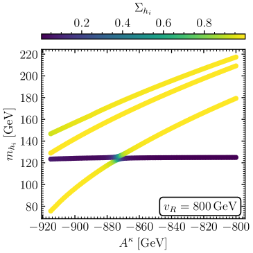
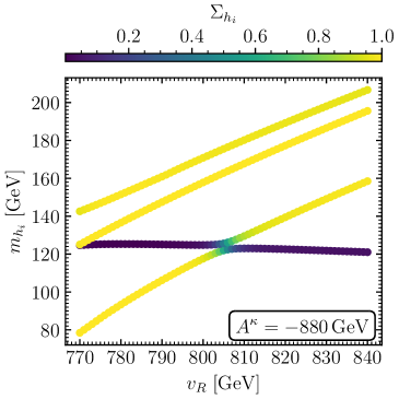
Figure 1: Masses of the Higgs bosons that are in the vicinity of $125\ \mathrm{GeV}$ as function of $A^{\kappa}$ (left) and $v_{R}$ (right). All points pass the HiggsBounds test. All points except the ones with $m_{h_{1}}\approx m_{h_{2}}\approx 125\ \mathrm{GeV}$ pass the HiggsSignals test (see text). The color coding indicates the gauge singlet component for each of the displayed Higgs bosons.

In Fig. 1 we show the radiatively corrected Higgs boson masses $m_{h_{1,...4}}$, corresponding to a SM-like Higgs boson at $\approx 125\ \mathrm{GeV}$ ($\equiv h_{125}$) and the three CP-even right-handed sneutrino states with masses not far below or above $125\ \mathrm{GeV}$. The colors of the points indicate the gauge singlet component of each Higgs boson, which we define as

$$\Sigma_{h_{i}}=\sum_{j=3}^{5}\left|R^{H}_{ij}\right|^{2}\ ,$$ (29)

where $R^{H}$ is the loop corrected mixing matrix that transforms the CP-even fields $\phi_{i}$ from the interaction basis into the fields $h_{i}$ in the mass eigenstate basis. One can see that, as expected from the discussion in Sect. 3.2, $h_{125}$ has only a small singlet component over almost the entire scan range, despite the fact that the right-handed sneutrinos are close in mass. The only exceptions are the points for which $h_{125}$ is practically degenerate with the lightest right-handed sneutrino and where a “level-crossing” occurs, i.e. $h_{125}$ changes its character from being the next-to-lightest state, $h_{2}=h_{125}$, to the lightest state, $h_{1}=h_{125}$. In the region where the level-crossing takes place the properties of a SM-like Higgs boson are in fact shared between the states $h_{1}$ and $h_{2}$, and both Higgs bosons contribute to the signal rate measurements at the LHC for the particle state at $\approx 125\ \mathrm{GeV}$.

Using HiggsSignals we applied a $\chi^{2}$-test to each parameter point shown in Fig. 1 in order to compare the predicted signal rates of $h_{125}$ with the experimental measurements. We discuss the results of this test in terms of $\Delta\chi^{2}=\chi^{2}_{\mu\nu{\rm SSM}}-\chi^{2}_{\rm SM}$, where $\chi^{2}_{\mu\nu{\rm SSM}}$ is the fit result of the parameter points and $\chi^{2}_{\rm SM}=84.4$ is the fit result assuming a SM Higgs boson at $125\ \mathrm{GeV}$. For the points of the scan over $A^{\kappa}$ (left plot of Fig. 1), we find a good compatibility with the measured properties of $h_{125}$, resulting in $\Delta\chi^{2}$ values of $\Delta\chi^{2}\approx-1$ to $3$, except for the points for which $m_{h_{1}}\approx m_{h_{2}}\approx 125\ \mathrm{GeV}$, where $\Delta\chi^{2}\approx 4$ to $6$. Here it should be noted that $A^{\kappa}$ does not appear in the alignment conditions. Accordingly, the variation of $A^{\kappa}$ does not have a sizable impact on the mixing of $h_{125}$ with the right-handed sneutrino states, except for the degenerate region with $m_{h_{1}}\approx m_{h_{2}}$, in which the assumptions on which the alignment condition rely are not fulfilled. Consequently, no sizable impact on the properties of $h_{125}$ is expected from the variation of $A^{\kappa}$ in the analyzed parameter space outside of the degenerate region.

The situation is different when $v_{R}$ is varied (right plot of Fig. 1), because it gives rise to a variation of the $\mu$ parameter that appears in Eq. (22). The constraint $\Delta\chi^{2}<6$ was used on the scan range, except for the points for which $h_{1}$ is degenerate with $h_{2}$, where we find values of $\Delta\chi^{2}$ of up to $\Delta\chi^{2}\approx 12$. Since we are mainly interested in the impact of the constraints on vacuum stability, and since the mass-degenerate points do not show any particular feature regarding the constraints from vacuum stability compared to the other points, we do not discard points with larger values of $\Delta\chi^{2}$ in the regions with $m_{h_{1}}\approx m_{h_{2}}\approx 125\ \mathrm{GeV}$ (we note that in this region the predicted signal rates, to which both $h_{1}$ and $h_{2}$ contribute, show sizable deviations from the measured values). For the upper end of the displayed $v_{R}$ range $\Delta\chi^{2}$ increases as a consequence of the decrease in the predicted value for the mass of the SM-like Higgs boson. For values of $v_{R}\gtrsim 830\ \mathrm{GeV}$ we find $m_{h_{125}}\lesssim 122\ \mathrm{GeV}$, which is outside of the allowed range that we have employed based on a theoretical uncertainty of the Higgs-mass prediction of $3\ \mathrm{GeV}$. The lower end of the scan range of $v_{R}$ arises from constraints from direct searches, as described below.

Regarding the HiggsBounds test, which confronts each parameter point with the available constraints from BSM Higgs-boson searches at colliders, all points of the scan over $A^{\kappa}$ pass the experimental constraints. This is related to the fact that the particles corresponding to the right-handed sneutrinos are very singlet-like and have strongly suppressed couplings to the SM particles. Only for the smallest values of $A^{\kappa}$ one can see an increase of the doublet component of the heaviest right-handed sneutrino ($h_{4}$), such that the channel $pp\to h_{4}\to ZZ^{*}$ becomes important, which was searched for by CMS in the two-lepton and four-lepton final states and including width effects [77]. However, the predicted cross sections remain roughly $20\%$ below the experimental limits even in this range of $A^{\kappa}$. The same experimental channel is also the most sensitive one in the scan over $v_{R}$, yielding an exclusion for values of $v_{R}<770\ \mathrm{GeV}$. Accordingly, we use this value as the lower limit of the scan over $v_{R}$.

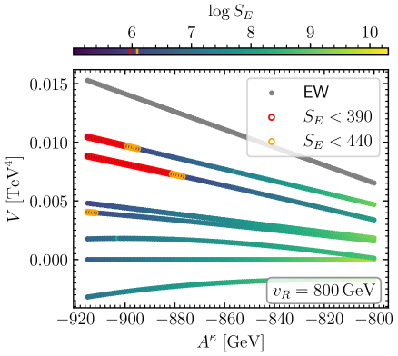
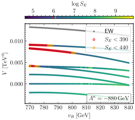
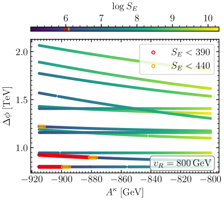
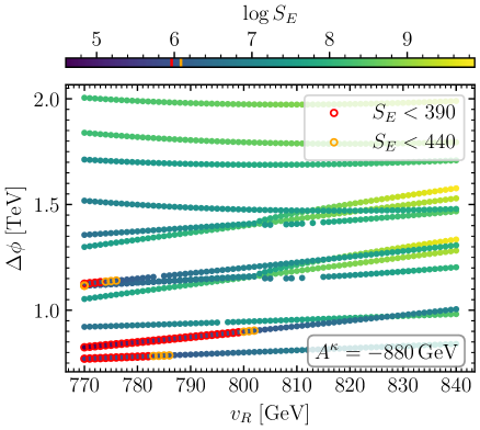
Figure 2: EW minimum and deeper unphysical minima as a function of $A^{\kappa}$ for fixed $v_{R}$ (left) and as a function of $v_{R}$ for fixed $A^{\kappa}$ (right). Shown are for each local minimum the potential values $V$ (top) and the field space distance between the unphysical minimum and the EW minimum $\Delta\phi$ (bottom). The colors of the points indicate the value of the euclidean bounce action $S_{E}$. Points with $S_{E}<390$ are highlighted with a red edge, while points with $390\leq S_{E}\leq 440$ are highlighted with an orange edge.

In Fig. 2 we show the results of the analysis of vacuum stability for the parameter space under investigation. On the left-hand side the points from the $A^{\kappa}$–scan are shown, and on the right hand side we show the points from the scan over $v_{R}$. In the upper row we show the values of the potential $V$ for the EW minimum and for all unphysical minima with potential values below the EW minimum. The points corresponding to the EW vacuum are shown in gray. For the unphysical minima the colors of the points indicate the values of the euclidean bounce action $S_{E}$ for the tunneling from the EW minimum into the unphysical minima. Parameter points for which we find that the EW vacuum is short-lived compared to the lifetime of the universe, corresponding to $S_{E}<390$, are furthermore highlighted in red. The regions with $390<S_{E}<440$, for which in our approach no clear distinction between a short-lived and a sufficiently long-lived vacuum can be drawn, are highlighted in orange (see the discussion in Sect. 4.2).

In both scans it can be observed that the EW minimum is not the global minimum of the potential for any of the points. In the $A^{\kappa}$–scan we find a total number of 12 deeper unphysical minima, where a few of those have the same depth $V$ due to the accidental symmetries mentioned in Sect. 2, such that only eight lines are visible in the upper left plot of Fig. 2. The situation is similar for the upper right plot, with the exception that for this scan the lines of two unphysical minima merge for small values of $v_{R}$. The different unphysical minima below the EW one can be more easily distinguished from each other in the plots displayed in the lower row where the field space distance between the unphysical minimum and the EW minimum, $\Delta\phi$, is shown. Here one can see for the $A^{\kappa}$–scan the already mentioned number of 12 unphysical minima below the EW one, while for the $v_{R}$–scan up to 14 unphysical minima below the EW one are visible. The lower right plot as a function of $v_{R}$ shows the interesting feature that for a certain value of $v_{R}\approx 803\ \mathrm{GeV}$ two of the unphysical minima bifurcate into two different ones each. Hence, in the $v_{R}$–scan either 12 or 14 unphysical minima below the EW minimum are present (see also the discussion below).

Even though there are numerous unphysical minima present below the EW vacuum for all the investigated parameter points, most of the unphysical minima do not give rise to a rapid decay of the EW vacuum, because the tunneling rates for all possible transitions turn out to be very small. This is in particular the case also for the global minimum of each parameter point, which is characterized by non-zero values of the right-handed sneutrino fields $\phi_{iR}$ and large negative values of the Higgs fields $\phi_{d}$ and $\phi_{u}$. As a result of the latter, the tunneling rates for transitions into the global minimum are suppressed by the large distance in field space between the EW minimum with positive values of $\phi_{d}$ and $\phi_{u}$.

The displayed results clearly indicate that a detailed investigation of the tunneling rates is crucial for determining the constraints from vacuum stability on the parameter space of the $\mu\nu$SSM. Analyses in which just the minima of the potential are determined and parameter points where the EW vacuum is not the global one are discarded, as they have sometimes been carried out in the literature for other models, would obviously be completely misleading for the case of the $\mu\nu$SSM.

As another interesting feature that is visible in Fig. 2, one can observe in the scan over $A^{\kappa}$ the presence of a local minimum with a vanishing potential value $V=0$ over the whole scan range. This minimum is located at the origin of field space, and it is therefore of particular interest. According to our approach for investigating vacuum stability, we find that the presence of this minimum at the origin of field space does not give rise to exclusions of parameter points in this scan, because the tunneling rate from the EW vacuum into this minimum is too small. It should however be noted that the analysis carried out here relies on the assumption that the EW minimum was actually adopted by the universe in its thermal history. If a local minimum at the origin exists in the universe now, one may wonder, however, whether such a local minimum at the origin may have existed already during the thermal history of the early universe. While in our present analysis of vacuum stability we restrict ourselves to the case of temperature $T=0$, a detailed analysis of the thermal history of the potential would be required in order to determine whether the EW vacuum was actually reached during the thermal evolution. Consequently, an analysis of the evolution of the field values as a function of the temperature (which is inversely proportional to the time) could potentially give rise to even stronger exclusion bounds compared to the zero-temperature analysis performed here (see also the discussion in Sect. 6). The minimum in the origin is also present for parts of the parameter space of the scan over $v_{R}$. It exists in the range $770\ \mathrm{GeV}\leq v_{R}\leq 802\ \mathrm{GeV}$, as can be seen in the upper right plot of Fig. 2. For larger values of $v_{R}$ the potential values bend down from the horizontal line at $V=0$ towards negative potential values, indicating that the minimum shifts away from the origin. The origin becomes unstable along the direction of $\phi_{u}$. Accordingly, in the range $803\ \mathrm{GeV}\leq v_{R}\leq 840\ \mathrm{GeV}$ we find an unphysical minimum with non-zero values of $53\ \mathrm{GeV}\leq|\phi_{u}|\leq 377\ \mathrm{GeV}$ and all other fields vanishing.

The above discussion leads to the following important conclusions. We have found that the $\mu\nu$SSM gives rise to a rich vacuum structure, featuring a metastable (i.e., long-lived in comparison to the age of the universe) or short-lived EW vacuum together with several deeper unphysical minima. Thus, the analysis of the validity of a certain parameter point should include a test of vacuum stability. Furthermore, as mentioned above, it would not be sufficient to simply require that the EW minimum is the global minimum of the potential, as such a criterion would exclude large parts of actually allowed parameter space. Instead, a calculation of the tunneling rates of the EW vacuum has to be performed in order to reliably determine whether a parameter point is phenomenologically viable. In the following we further discuss the structure of the potentially dangerous unphysical minima, including an analytical discussion of the dependence on the main parameters entering the calculation of $S_{E}$, in order to determine which parts of the $\mu\nu$SSM parameter space are expected to be susceptible to vacuum instabilities.

We note in this context that parameter points where the EW vacuum is short-lived feature transitions into unphysical minima which are not the deepest ones. On the contrary, we can see from the plots in the upper row of Fig. 2 that the most dangerous minima are in fact the ones with the highest values of $V$, which therefore have the smallest potential difference compared to the EW minimum, $\Delta V_{\rm EW}$. This indicates that for the considered case $\Delta V_{\rm EW}$ is not the most important quantity in the evaluation of the transition rate. Instead, as can be seen in the lower row of Fig. 2, the distance in field space $\Delta\phi=|\phi_{\rm EW}-\phi|$ between the EW minimum at $\phi_{\rm EW}$ and an unphysical minimum at $\phi$ has a bigger impact. In the lower row of Fig. 2, $\Delta\phi$ is shown as a function of $A^{\kappa}$ on the left and of $v_{R}$ on the right for all potentially dangerous (i.e., deeper than the EW vacuum) unphysical minima that occur for each parameter point. It can be seen that the transitions with the lowest values of $S_{E}$ are typically those into the unphysical minima with the lowest values of $\Delta\phi$ (as expected, a smaller distance in field space is correlated with a higher decay rate of the EW vacuum). Our results indicate that for the analyzed $\mu\nu$SSM scenarios the distance in field space is more important for the determination of the tunneling rate of the EW vacuum than the difference of the potential depths.

In the lower right plot of Fig. 2, and to a lesser extent also in the lower left plot, one can see that a few points are missing in the curves (in particular near the bifurcation point in the lower right plot). This is due to the fact that the numerical approach applied here to determine the stationary conditions missed one of the minima (see also the discussion in Sect. 4.1). Nevertheless, given the fact that this happened only in rare cases, our conclusions regarding the impact of vacuum stability constraints on the $\mu\nu$SSM are not affected by this issue. In practice, it was always possible to find also the minima missing in Fig. 2 by marginally changing the input parameters. However, we decided to show the results as they were obtained during a single run in order to give an impression of the performance of the applied procedure.

	$A^{\kappa}$	$v_{R}$	$\phi_{d}$	$\phi_{u}$	$\phi_{1R}$	$\phi_{2R}$	$\phi_{3R}$	$\phi_{1L}/10^{-4}$	$\phi_{2L}/10^{-4}$	$\phi_{3L}/10^{-4}$
AI	$-880$	$800$	$115.3$	$230.9$	$803.7$	$801.1$	$-0.4755$	$1.053$	$1.050$	$-0.000642$
AII			$156.2$	$515.7$	$-25.18$	$992.0$	$804.8$	$-0.01805$	$2.259$	$2.167$
BI	$-900$	$800$	0	0	0	0	$800.0$	0	0	0
BII			$162.8$	$530.0$	$-25.65$	$1014$	$-0.2768$	$-0.01578$	$2.718$	$-0.00027$
BIII			$165.6$	$534.3$	$-27.45$	$1017$	$806.6$	$-0.0202$	$2.752$	$2.263$
BIV			$115.5$	$230.9$	$806.1$	$800.7$	$-0.4541$	$1.057$	$1.050$	$-0.00061$
CI	$-880$	$780$	0	0	0	0	$779.9$	0	0	0
CII			$115.5$	$230.6$	$788.9$	$781.0$	$-0.4449$	$1.059$	$1.0502$	$-0.00061$
CIII			$135.6$	$449.8$	$-13.08$	$958.5$	$-0.159$	$0.00472$	$2.215$	$-0.00006$
CIV			$138.9$	$455.6$	$-14.48$	$961.9$	$785.2$	$0.00235$	$2.256$	$1.902$
EW		$v_{R}$	$110.1$	$220.2$	$v_{R}$	$v_{R}$	$v_{R}$	$1$	$1$	$1$

Table 2: Field values of unphysical local minima for which $S_{E}<700$ are given for three selected parameter points. The last row shows the field values of the EW minimum, which are the same for the three parameter points. Dimensionful parameters and field values are given in GeV.

The fact that the field space distance $\Delta\phi$ appears to be more important than the potential difference $\Delta V_{\rm EW}$, and also that the dangerous minima were found at distances $\Delta\phi\approx v_{R}$, makes it apparent that the field values of the right-handed sneutrino fields are particularly important for the determination of the tunneling rates. In order to shed more light on the field configurations of the unphysical minima, we show in Tab. 2 the field values of the most dangerous minima for three selected parameter points together with the field values of the EW minimum ($\phi_{d}$ and $\phi_{u}$ in the EW minimum are determined by $\tan\beta=2$ and $v\approx 246\ \mathrm{GeV}$). We only display the unphysical minima for which the transition rate from the EW minimum corresponds to values of $S_{E}$ below $700$. The first parameter point under consideration (A) has $A^{\kappa}=-880\ \mathrm{GeV}$ and $v_{R}=800\ \mathrm{GeV}$, and it features the unphysical minima AI and AII with $S_{E}<700$. The most striking feature of these minima is that, while the EW minimum has universal field values $\phi_{iR}=v_{R}$, in AI and AII the field value of one of the right-handed sneutrino fields is almost zero, while the other two approximately maintain values of about $v_{R}$. A similar observation can be made for the second parameter point (B), with $A^{\kappa}=-900\ \mathrm{GeV}$ and $v_{R}=800\ \mathrm{GeV}$, featuring the unphysical minima BI–BIV. Here, the minima BIII and BIV are the analogues to the minima AII and AI of the first parameter point, respectively, i.e. they lie on the same branch of points in the plots in Fig. 2. In addition, two more minima are shown for the parameter point B, where only one of the fields $\phi_{iR}$ has a value of $\approx v_{R}$, while the other two have $\phi_{iR}\approx 0$. For example, BI lies exactly on the $\phi_{3R}$ axis. Two minima of this kind are also present for the parameter point A, but they correspond to EW vacuum decay rates with $S_{E}>700$ and are therefore not shown in the table. The second point has a larger value of $|A^{\kappa}|$. This suggests that more negative values of $A^{\kappa}$ can give rise to an unstable EW vacuum (as also shown in Fig. 2). Finally, the third point (C) with $A^{\kappa}=-880\ \mathrm{GeV}$ and $v_{R}=800\ \mathrm{GeV}$ features the unphysical minima CI–CIV. While they show a similar field configuration as BI–BIV, it is interesting to compare the different parameters related to the tunneling probabilities.

	$\Delta\phi$	$m(\hat{\varphi})$	$A(\hat{\varphi})$	$\lambda(\hat{\varphi})$	$-\Delta V_{\mathrm{EW}}^{1/4}$	$S_{E}$
AI	$800.6$	$106.2$	$58.71$	$0.0462$	$250.2$	$660.0$
AII	$898.4$	$83.81$	$45.28$	$0.03345$	$270.8$	$\mathbf{401.5}$
BI	$1158$	$91.35$	$39.44$	$0.02244$	$313.9$	$675.6$
BII	$1211$	$81.73$	$34.37$	$0.01901$	$319.1$	$609.2$
BIII	$912.9$	$70.21$	$42.26$	$0.0318$	$278.1$	$\mathbf{241.1}$
BIV	$800.6$	$94.07$	$56.68$	$0.04620$	$258.1$	$\mathbf{380.4}$
CI	$1130$	$86.97$	$38.34$	$0.02248$	$308.1$	$610.9$
CII	$780.6$	$90.08$	$55.01$	$0.04619$	$252.6$	$\mathbf{353.89}$
CIII	$1150$	$77.41$	$34.34$	$0.02013$	$308.8$	$516.1$
CIV	$848.8$	$64.43$	$42.97$	$0.0351$	$266.9$	$\mathbf{180.7}$

Table 3: Values for the coefficients $m$, $A$ and $\lambda$ as defined in Eq. (26) for the non-EW minima shown in Tab. 2. Also shown are the distance in field space $\Delta\phi$ and the potential difference $-\Delta V_{\rm EW}^{1/4}$ between the EW minimum and the unphysical minima. The last column shows the euclidean bounce action $S_{E}$ for the transitions. Values of $S_{E}$ giving rise to a (potentially) short-lived EW vacuum are given in bold font. Dimensionful parameters and field values are given in GeV.

For this reason we show in Tab. 3 the values of $S_{E}$ associated to each minimum, together with the coefficients that define the form of $V_{\rm EW}$ as defined in Eq. (26). Values of $S_{E}$ giving rise to a (potentially) short-lived EW vacuum are highlighted in bold font. In addition, the table also lists the values for the field space distance $\Delta\phi$ and the potential difference $-\Delta V_{\rm EW}$ between the EW minimum and the unphysical minima. One can see that all three points have at least one unphysical deeper minimum associated with a value of $S_{E}<440$. For AII we find $S_{E}=401.5$, such that for the parameter point A the EW vacuum is potentially short-lived. In order to definitively answer the question whether point A features a sufficiently long-lived EW vacuum or not, one would have to improve the computation of $S_{E}$, incorporating in particular a more elaborate treatment of the prefactor $K$ introduced in Eq. (28) (see also the discussion below). For the parameter point B, the presence of both BIII and BIV with $S_{E}=241.1$ and $S_{E}=380.4$, respectively, indicates that the EW vacuum is short-lived, and the parameter point should be rejected. The same observation can be made for the parameter point C, for which we find $S_{E}=353.89$ for CII and $S_{E}=180.7$ for CIV.

One can gain further analytical insight into the tunneling dynamics by comparing the minima of different parameter points with similar field configurations, i.e. minima that lie on the same branch of points in Fig. 2. As already mentioned before, for the point A with the minimum AI and $S_{E}=660.0$ the analogues minimum for the point B is the minimum BIV with $S_{E}=380.4$. Hence, the change from $A^{\kappa}=-880\ \mathrm{GeV}$ to $A^{\kappa}=-900\ \mathrm{GeV}$ gives rise to an instability of the EW vacuum. The reason for this can be understood analytically by realizing that the only field that substantially changes if the EW vacuum decays into AI and BIV is $\phi_{3R}$. In the EW minium we have $\phi_{3R}=v_{R}=800\ \mathrm{GeV}$, and the field evolves to $\phi_{3R}\approx 0$ during the transition. Thus, the potential $V_{\rm EW}$ as defined in Eq. (26) is given for this kind of transitions in very good approximation by choosing the unit field vector $\hat{\varphi}_{i}$ in the direction of $-\phi_{3R}$, such that $\hat{\varphi}_{\rm AI,BIV}=(0,0,0,0,-1,0,0,0)$. Then the coefficients of $\Delta V_{\rm EW}$ are given by

$$A(\hat{\varphi}_{\rm AI,BIV}) =\kappa_{3}\left(\frac{1}{3\sqrt{2}}A^{\kappa}_{3}+\kappa_{3}v_{3R}\right)\ ,$$ (30)

$$m^{2}(\hat{\varphi}_{\rm AI,BIV}) =\frac{\lambda_{3}v^{2}}{8v_{3R}}\left(\sqrt{2}A^{\lambda}_{3}s_{2\beta}-2\left(\lambda_{1}v_{1R}+\lambda_{2}v_{2R}\right)\right)+\frac{1}{4}\kappa_{3}v_{3R}\left(\sqrt{2}A^{\kappa}_{3}+4\kappa_{3}v_{3R}\right)\ ,$$ (31)

$$\lambda(\hat{\varphi}_{\rm AI,BIV}) =\frac{1}{4}\kappa_{3}^{2}\ ,$$ (32)

where in the second row the terms $\sim v_{iL}$ and $\sim Y^{\nu}_{ij}$ were neglected, and where in our scans $v_{R}=v_{1R}=v_{2R}=v_{3R}$. Furthermore, given the small value of $\lambda_{3}=0.05$ in this scenario, the first term in the expression for $m^{2}$ is suppressed compared to the second term. For the determination of $S_{E}$ the ratio $A^{2}/(m^{2}\lambda)$ is particularly important (see also the definition of $\delta$ in Eq. (27)), which is related to the fact that terms in $V_{\rm EW}$ with odd powers of the fields give rise to the potential barrier that separates the EW minimum from the unphysical minimum: increasing the trilinear coefficient $A$ leads to larger values of $S_{E}$, while $S_{E}$ becomes smaller with increasing coefficients $m^{2}$ and $\lambda$ of the terms with even powers of the fields. Focusing on the terms $\sim A^{\kappa}_{3}$, we find that this ratio scales with $-\kappa_{3}|A^{\kappa}_{3}|/v_{R}$. Thus, if $|A^{\kappa}_{3}|$ becomes larger, the decrease in the potential barrier caused by $A$ is more important than the decrease of the bilinear coefficient $m^{2}$, such that $S_{E}$, and therefore the lifetime of the EW vacuum, becomes smaller.

It should be noted that the change from an unstable to a metastable EW vacuum sensitively depends on the value of $A^{\kappa}$, as we demonstrated here for the points A and B, where the $A^{\kappa}$ values differ by only $\approx 2\%$ for points with a metastable and an unstable vacuum. Consequently, one can expect that the uncertainty that is related to our treatment of the prefactor $K$ in Eq. (28), giving rise to the intermediate regime $390<S_{E}<440$ in which the lifetime of the EW vacuum is of comparable size as the age of the universe, affects only a relatively small fraction of the $\mu\nu$SSM parameter space. For most parts of the parameter space, the value of $S_{E}$ for possible vacuum decays should either be substantially below or above the intermediate regime with $S_{E}\approx 400$, such that its impact on vacuum stability can clearly be determined.

The smallest values of $S_{E}$ are found for the parameter point C, which has a smaller value of $v_{R}=780\ \mathrm{GeV}$ compared to $v_{R}=800\ \mathrm{GeV}$ for the points A and B. We already mentioned before that this can intuitively be understood due to the fact that the field space difference $\Delta\phi$ becomes smaller for the relevant unphysical minima. We find, for example, a value of $S_{E}=353.89$ for the minimum CII, while for the analogous minimum AII of the first parameter point with an identical value of $A^{\kappa}$ we find $S_{E}=401.5$. Following the above reasoning, the smaller $S_{E}$ value for CII compared to AII can be understood by the fact that (for $\lambda_{3}\ll 1$) $A^{2}/(m^{2}\lambda)$ scales with $1/v_{R}$. Comparing to Tab. 3, one can additionally see that also the absolute value of the potential difference $|\Delta V_{\rm EW}|$ changes with $v_{R}$. However, since the rate for the vacuum decay into CII is larger compared to the decay into AII, even though $|\Delta V_{\rm EW}|$ is larger for AII, one can conclude (as before) that the field space difference $\Delta\phi$ has quantitatively a larger impact on the lifetime of the EW vacuum.

The most dangerous minima of all three parameter points cause EW vacuum decays for which $\phi_{1R}$ (instead of $\phi_{3R}$) evolves from $\phi_{1R}=v_{R}$ to $\phi_{1R}\approx 0$. For these transitions an important difference arises from the fact that $\lambda_{1}=0.56\gg\lambda_{3}$, such that the interactions between $\phi_{1}$ and the Higgs doublet fields $\phi_{d}$ and $\phi_{u}$ cannot be neglected. As a result, also the latter fields change during the transition from the EW vacuum into the vacua AII, BIII and CIV, while $\phi_{d}$ and $\phi_{u}$ remain approximately constant for the transitions into AI, BIV and CII. For the cases where the doublet fields change during the transition, the expressions for the coefficients of $V_{\rm EW}$ become significantly more complicated and the analytic treatment does not provide much insight. Instead we show in Fig. 3 the potential difference $\Delta V_{\rm EW}$ in the direction of the unphysical minimum corresponding to the smallest value of $S_{E}$ for different values of $A^{\kappa}$ and $v_{R}$.

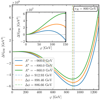
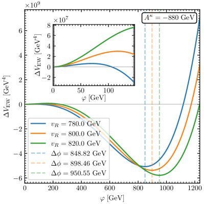
Figure 3: $\Delta V_{\rm EW}$ along the straight path connecting the EW minimum and the most dangerous unphysical minimum for different values of $A^{\kappa}_{i}$ (left) and $v_{iR}$ (right). Also indicated are the field space distances $\Delta\phi$ with vertical dashed lines.

In the left plot of Fig. 3 we show the potential difference $\Delta V_{\rm EW}$ for three different values of ${A^{\kappa}=-900,-880,-860\ \mathrm{GeV}}$ and for fixed $v_{R}=800\ \mathrm{GeV}$, while the remaining parameters are fixed as shown in Tab. 1. Hence, the curve with $A^{\kappa}=-880\ \mathrm{GeV}$ (orange) corresponds to the parameter point A discussed in relation to Tab. 2 and Tab. 3, and $\Delta V_{\rm EW}$ is shown in the direction of the minimum AII. One can see that the variation of $A^{\kappa}$ induces a variation of both the barrier height and the depth of the unphysical minimum, whereas the field space difference $\Delta\phi$ (indicated by the vertical dashed lines) is largely unaffected. This follows the expectation from Eq. (30): For a transition which at least partially evolves in the direction ${-\phi_{iR}\ ,\ i=1,2,3}$, there is a positive contribution to the coefficient $A$ which is proportional to $v_{iR}\kappa_{i}^{2}$, and a negative contribution proportional to $-\kappa_{i}|A^{\kappa}_{i}|$. Thus, the smaller $|A^{\kappa}|$, the larger is the potential barrier between both minima for fixed values of $v_{iR}$ and $\kappa_{i}$, and the lifetime of the EW vacuum increases. On the other hand, for large values of $|A^{\kappa}_{i}|$ the lifetime of the EW vacuum decreases, and constraints arising from the vacuum stability become important.

This observation is not surprising since it is known that for $|A^{\kappa}_{i}|\gg v_{iR}\kappa_{i}$ the CP-even right-handed sneutrinos can become tachyonic [23, 32], pointing to the fact that vacuum instabilities might occur. Similar observations were also made in the NMSSM where only one gauge singlet field is present [78, 40]. In the $\mu\nu$SSM, the presence of three such fields leads to the fact that there are more ways in which dangerous unphysical minima can arise. For instance, there can be minima in which one, two or all three fields $\phi_{iR}$ take on values of $\approx 0$. In addition, the way in which the singlet states are coupled to the doublet Higgs fields yields a much richer structure of vacuum configurations, with several options that could give rise to EW vacuum instabilities. Thus, compared to the NMSSM, the constraints from vacuum instabilities can be expected to be even more important in the $\mu\nu$SSM.

In the right plot of Fig. 3 we show $\Delta V_{\rm EW}$ in the direction of the most dangerous unphysical minimum for different values of ${v_{R}=780,800,820\ \mathrm{GeV}}$ and a fixed value of $A^{\kappa}=-880\ \mathrm{GeV}$. As before, the orange curve belongs to the parameter point A of Tab. 2, with $\Delta V_{\rm EW}$ shown in the direction of the minimum AII. There are two main effects of the variation of $v_{R}$ on the stability of the EW vacuum. As already mentioned before, smaller values of $v_{R}$ reduce the value of $\Delta\phi$ (indicated by the vertical dashed lines in Fig. 3) for minima of the type shown in Tab. 2, in which the field values of one or more right-handed sneutrinos go from $v_{R}$ to zero during the transition. Hence, smaller values of $v_{R}$ are also associated with a smaller lifetime of the (metastable) EW vacuum. This effect is further enhanced by the fact that also the potential barrier becomes smaller when the value of $v_{R}$ becomes smaller.

In combination of both observations discussed above, i.e., smaller values of $v_{iR}$ and larger values of $|A^{\kappa}_{i}|$ can lead to an unstable EW vacuum, there is a clear phenomenological consequence. One can expect that an instability of the EW vacuum in the $\mu\nu$SSM can be caused by the presence of relatively light right-handed sneutrinos, with masses at or below the EW scale. Since this is the parameter region in which there are prospects to potentially probe the existence of these particle states at the LHC or other future colliders, either directly or indirectly via signal rate measurements of the Higgs boson at $125\ \mathrm{GeV}$, the constraints from vacuum stability can have an important impact on scenarios that can be probed by collider experiments, and thus should be taken into account in analyses of the collider prospects of the $\mu\nu$SSM.

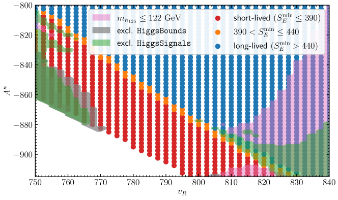
Figure 4: Vacuum stability constraints in the $v_{R}$-$A^{\kappa}$ plane. Blue points feature a sufficiently long-lived EW vacuum, while the red points give rise to a rapidly decaying EW vacuum. The orange points feature a potentially short-lived EW vacuum (see text). The gray and green areas indicate excluded regions based on the HiggsBounds and HiggsSignals constraints (see text for details), and the pink area indicates the parameter region in which $m_{h_{125}}<122\ \mathrm{GeV}$.

As an illustration of our results, we show in Fig. 4 the parameter points in the $v_{R}$-$A^{\kappa}$ plane, in which the parameter space is divided into a red region in which the EW vacuum is short-lived, an orange region in which the EW vacuum is potentially short-lived (see the discussion in Sect. 4.2 about this intermediate region), and a blue region in which the EW vacuum is metastable and long-lived. There are no points in the lower left corner due to the appearance of tachyonic CP-even states at tree level (see also Fig. 1). For none of the points the EW minimum is the global minimum of the potential. Demanding that the EW minimum should be the global minimum would imply the exclusion of the phenomenologically viable blue region. This illustrates the importance of taking into account the possibility of a sufficiently long-lived metastable EW vacuum. Since the lifetime of the EW vacuum has a sensitive dependence on the precise values of $v_{R}$ and $A^{\kappa}$, the orange region constitutes only a small narrow band of the investigated parameter space. As the parameter points in the red region feature a short-lived EW vacuum, they are not physically viable and should be excluded.

The lightest (loop-corrected) scalar masses that we find in the red, blue and orange regions are $m_{h_{1}}=70.77\ \mathrm{GeV},112.4\ \mathrm{GeV}$ and $116.5\ \mathrm{GeV}$, respectively. As a result, we find that in this scenario all points with $m_{h_{1}}<112\ \mathrm{GeV}$ are excluded due to EW vacuum stability constraints. This demonstrates the importance of the interplay between the constraints from vacuum stability and possible collider phenomenology of the model at current or future colliders. As is indicated by the gray area, only two small parameter regions are excluded via cross section limits from direct searches, and both of these regions lie within the red parameter region. Hence, we observe in the scenario investigated here that the vacuum stability constraints have a larger impact and give rise to exclusion limits that by far exceed the present limits from direct searches for the BSM Higgs bosons of the $\mu\nu$SSM.

In Fig. 4 we also indicate the parameter points for which the prediction for the mass of the SM-like Higgs-boson does not lie within the range $(125\pm 3)\ \mathrm{GeV}$ (pink area). However, the points in this region should not be considered as strictly excluded, since $m_{h_{125}}$ could easily be adjusted to lie within the required interval by modifying the parameters related to the stop sector, from which the radiative corrections to $m_{h_{125}}$ mainly arise. Related to $m_{h_{125}}$, one can also see that large parts of the green area, which indicates a worse fit to the signal-rate measurements of $h_{125}$, overlap with the pink area. The green area is defined as the parameter region in which the points have $\Delta\chi^{2}=\chi^{2}_{\mu\nu{\rm SSM}}-\chi^{2}_{\rm SM}>5.99$, i.e. the points are disfavored at the $95\%$ confidence level in the two-dimensional parameter scan considered here. In contrast to the exclusions from direct searches, the exclusion limits related to the properties of $h_{125}$ (pink and green areas) stretch out over parts of the blue parameter region.

6 Conclusions and outlook

In this paper we have presented an investigation of the stability of the EW vacuum of the $\mu\nu$SSM. We have described in detail the approach that was used in order to determine the dangerous unphysical minima in the eight-dimensional field space of the CP-even scalar fields. Moreover, we have utilized a numerically robust semi-classical approximation for the computation of the EW vacuum decay rates, which allowed us to categorize parameter points for which the EW minimum is not the global minimum into points featuring a metastable long-lived or an unstable EW vacuum (as well as an intermediate region between the two cases).

Focusing on the alignment without decoupling limit of the model, we have demonstrated in our numerical discussion how the analysis of vacuum stability can provide important constraints on the parameter space. We have generically found that the EW minimum is not the global minimum of the potential. In comparison to the NMSSM, the presence of three gauge singlet scalar fields in the $\mu\nu$SSM leads to the possibility of various potentially dangerous unphysical minima existing in the neutral scalar potential for a single parameter point. We have found that the largest rates of the EW vacuum decays are related to the unphysical minima that are the closest in field space to the EW minimum, despite the fact that there might be even deeper unphysical minima present. Furthermore, our results clearly indicate that simply requiring that the EW minimum is the global minimum of the potential would exclude large parts of the $\mu\nu$SSM parameter space that are actually phenomenologically viable. Instead, it is crucial to take into account the possibility of a metastable EW vacuum and to perform an analysis of the EW vacuum decay rates.

We have shown analytically and numerically that an unstable EW vacuum can be expected to occur quite generically in regions of the parameter space in which relatively light right-handed sneutrinos are present. Due to the fact that these particles are gauge singlets, thus not coupled directly to the SM particles, they may not be detectable at collider experiments even if they have small masses. It is therefore an important finding that the corresponding parameter space can be constrained in other ways, such as the vacuum stability investigation as presented here. On the other hand, for the case where the sneutrinos have a significant coupling to the SM particles via a mixing with the Higgs boson at $125\ \mathrm{GeV}$, constraints from collider experiments in combination with constraints from the analysis of the EW vacuum stability can be utilized in a complementary way in order to exclude parts of the parameter space of the $\mu\nu$SSM.

As an outlook to possible future research, we emphasize that further constraints on the parameter space of the $\mu\nu$SSM may be obtained by complementing the present analysis at $T=0$ with an investigation of the thermal history of the universe, see recent studies in other scalar extensions of the SM [40, 41]. While the EW minimum might be sufficiently long-lived at zero temperature, the universe might have adopted one of the unphysical minima during its thermal history. It can then happen that the transition rate for the phase transition into the EW vacuum would have never been large enough to allow for the onset of EW symmetry breaking, and the universe would have been trapped until zero temperature in one of the unphysical minima. This vacuum trapping effect is especially important if the formation of vacua at the origin, or vacua in which only the singlet fields obtain vacuum expectation values, are possible, and we encountered such cases in our analysis. It should be noted that minima of the latter kind usually form at temperatures much larger than the EW scale, because vanishing field values of the singlet fields are not stabilized via the SM interactions. In the event that an unphysical minimum at the origin (or any minimum that features non-zero vevs only for the right-handed sneutrino fields) can exist until zero temperature there are then two possibilities: The universe is trapped in such a vacuum, or the universe undergoes a first-order EW phase transition. While the vacuum trapping might yield important constraints on the parameter space of the $\mu\nu$SSM, the possibility of first-order EW phase transitions can facilitate baryogenesis or give rise to the formation of a stochastic gravitational wave background in the early universe, thus pointing towards particularly interesting regions of parameter space. An investigation of the thermal history of the $\mu\nu$SSM is left for future work.

Appendix A Checking vacuum stability with munuSSM

The determination of the unphysical minima and the computation of the lifetime of (metastable) EW vacuum in the $\mu\nu$SSM can be performed with the new version of the public code munuSSM. The implementation follows the approach described in Sect. 4, which is based on Ref. [37]. The stationary conditions are solved with an interface to the public code Hom4PS2 [47]. We briefly summarize here the usage of the code employed for the analysis presented in Sect. 5, including a description of the user interface of the new vacuum stability test. A more detailed account of the user interface can be found in the documentation under https://www.desy.de/~biek/munussmdocu/site/.

Assuming that there is an input file called path in which the values for the free parameters are defined (see Ref. [34] for details), the corresponding parameter point can be analyzed by executing the commands:

⬇

from munuSSM.benchmarkPointFromFile import \

BenchmarkPointFromFile

from munuSSM.vacuumStability.checkPotential import \

CheckPotential

from munuSSM.higgsBounds.util import \

check_higgsbounds_higgssignals

pt = BenchmarkPointFromFile(file=’path’)

pt.calc_loop_masses()

checker = CheckPotential(pt)

checker.check_stability()

check_higgsbounds_higgssignals(pt)

The results of the HiggsBounds and the HiggsSignals test are then saved in the dictonaries:

⬇

pt.HiggsBounds

pt.HissSignals

The definition of each item of the dictionaries can be found in Ref. [34]. The most time-consuming call is the one of the function check_stability, which depending on the input parameters usually takes roughly a minute to finish. The results of the vacuum stability check are saved in:

⬇

pt.local_minima

pt.Transitions

The attribute local_minima is a list of dictionaries, where each dictionary saves the field values $\phi_{d}$ and the potential depth $V(\phi_{d})$ of each local minimum. The attribute Transitions is also a list of dictionaries, where each dictionary saves the relevant information about the possible transitions into each deeper unphysical minimum $\phi_{d}$. These dictionaries have the following items:

• ’DangMin’: $\phi_{d}$

• ’V’: $V(\phi_{d})$

• ’unitvec’: $\hat{\varphi}_{d}$

• ’unit_min_pos’: $\Delta\phi_{d}$

• ’msq’: $m^{2}(\hat{\varphi}_{d})$

• ’A’: $A(\hat{\varphi}_{d})$

• ’lambda’: $\lambda(\hat{\varphi}_{d})$

• ’delta’: $\delta(\hat{\varphi}_{d})$

• ’Action’: $S_{E}$

As discussed in Sect. 4, a parameter point can be considered to be valid if all values of $S_{E}$ are larger than $440$. If the attribute Transitions is empty, then there are no unphysical minima below the EW minimum, and the point is also valid.

Appendix B Coefficients of $V_{\rm EW}$ for special cases

We consider here two special cases, for which we provide explicit expressions for the coefficients of the scalar potential relative to the EW vacuum, $V_{\rm EW}(\varphi,\hat{\varphi})$, as given in Eq. (26). If one of the right-handed sneutrino fields $\phi_{iR}$ is mixed with the SM-like Higgs boson, then transitions along the directions $-\phi_{iR}$ and $\phi_{u}$ occur (see AII, BIII and CIV in Tab. 2). Choosing for instance $i=1$, the unit vector $\hat{\varphi}$ for such transitions can be approximately expressed as

$$\hat{\varphi}=N\left(0,D,1/D,0,0,0,0,0\right)\ ,\;\text{with}\;N=\frac{D}{\sqrt{D^{4}+1}}\ ,$$ (33)

where $D$ parametrizes the direction in field space, and the variation of the other fields was neglected. Then the coefficients of $V_{\rm EW}$ are given by

$$m^{2}=-\frac{\lambda_{1}\lambda_{2}N^{2}v^{2}c_{\beta}^{2}v_{2R}}{4D^{2}v_{1R}}-\frac{\lambda_{1}\lambda_{2}N^{2}v^{2}s_{\beta}^{2}v_{2R}}{4D^{2}v_{1R}}-\frac{\lambda_{1}\lambda_{3}N^{2}v^{2}c_{\beta}^{2}v_{3R}}{4D^{2}v_{1R}}-\frac{\lambda_{1}\lambda_{3}N^{2}v^{2}s_{\beta}^{2}v_{3R}}{4D^{2}v_{1R}}+\frac{\lambda_{1}N^{2}v^{2}A_{1}^{\lambda}c_{\beta}s_{\beta}}{2\sqrt{2}D^{2}v_{1R}}+\frac{D^{2}\lambda_{1}N^{2}A_{1}^{\lambda}c_{\beta}v_{1R}}{2\sqrt{2}s_{\beta}}+\frac{\kappa_{1}N^{2}A_{1}^{\kappa}v_{1R}}{2\sqrt{2}D^{2}}+\frac{D^{2}\kappa_{1}\lambda_{1}N^{2}c_{\beta}v_{1R}^{2}}{4s_{\beta}}+\kappa_{1}\lambda_{1}N^{2}vc_{\beta}v_{1R}+\frac{\kappa_{1}^{2}N^{2}v_{1R}^{2}}{D^{2}}-\lambda_{1}^{2}N^{2}vs_{\beta}v_{1R}+\frac{D^{2}\lambda_{2}N^{2}A_{2}^{\lambda}c_{\beta}v_{2R}}{2\sqrt{2}s_{\beta}}+\frac{D^{2}\kappa_{2}\lambda_{2}N^{2}c_{\beta}v_{2R}^{2}}{4s_{\beta}}-\lambda_{1}\lambda_{2}N^{2}vs_{\beta}v_{2R}+\frac{D^{2}\lambda_{3}N^{2}A_{3}^{\lambda}c_{\beta}v_{3R}}{2\sqrt{2}s_{\beta}}+\frac{D^{2}\kappa_{3}\lambda_{3}N^{2}c_{\beta}v_{3R}^{2}}{4s_{\beta}}-\lambda_{1}\lambda_{3}N^{2}vs_{\beta}v_{3R}+\frac{\lambda_{1}N^{2}vA_{1}^{\lambda}c_{\beta}}{\sqrt{2}}+\frac{1}{8}D^{2}g_{1}^{2}N^{2}v^{2}s_{\beta}^{2}+\frac{1}{8}D^{2}g_{2}^{2}N^{2}v^{2}s_{\beta}^{2}\ ,$$ (34)

$$A=\frac{\kappa_{1}^{2}N^{3}v_{1R}}{D^{3}}+\frac{\kappa_{1}N^{3}A_{1}^{\kappa}}{3\sqrt{2}D^{3}}+\frac{\kappa_{1}\lambda_{1}N^{3}vc_{\beta}}{2D}+\frac{1}{2}D\lambda_{1}\mu N^{3}-\frac{\lambda_{1}^{2}N^{3}vs_{\beta}}{2D}\ ,$$ (35)

$$\lambda=\frac{1}{32}D^{4}g_{1}^{2}N^{4}+\frac{1}{32}D^{4}g_{2}^{2}N^{4}+\frac{\kappa_{1}^{2}N^{4}}{4D^{4}}+\frac{1}{4}\lambda_{1}^{2}N^{4}\ .$$ (36)

Another kind of transition that was encountered in the numerical discussion was one in which two of the right-handed sneutrino fields, e.g., $\phi_{1R}$ and $\phi_{2R}$, evolve from $v_{R}$ to approximately zero (see BI and CI in Tab. 2). Neglecting the variation of the Higgs doublet fields $\phi_{d}$ and $\phi_{u}$ for these transitions, one can parametrize the unit vector by

$$\hat{\varphi}=-N\left(0,0,D,1/D,0,0,0,0\right)\ ,$$ (37)

and one finds for the coefficients

$$m^{2}=-\frac{D^{2}\lambda_{1}\lambda_{2}N^{2}v^{2}c_{\beta}^{2}v_{2R}}{4v_{1R}}-\frac{\lambda_{1}\lambda_{2}N^{2}v^{2}c_{\beta}^{2}v_{1R}}{4D^{2}v_{2R}}-\frac{D^{2}\lambda_{1}\lambda_{2}N^{2}v^{2}s_{\beta}^{2}v_{2R}}{4v_{1R}}-\frac{\lambda_{1}\lambda_{2}N^{2}v^{2}s_{\beta}^{2}v_{1R}}{4D^{2}v_{2R}}-\frac{D^{2}\lambda_{1}\lambda_{3}N^{2}v^{2}c_{\beta}^{2}v_{3R}}{4v_{1R}}-\frac{D^{2}\lambda_{1}\lambda_{3}N^{2}v^{2}s_{\beta}^{2}v_{3R}}{4v_{1R}}+\frac{D^{2}\lambda_{1}N^{2}v^{2}A_{1}^{\lambda}c_{\beta}s_{\beta}}{2\sqrt{2}v_{1R}}+\frac{D^{2}\kappa_{1}N^{2}A_{1}^{\kappa}v_{1R}}{2\sqrt{2}}+D^{2}\kappa_{1}^{2}N^{2}v_{1R}^{2}-\frac{\lambda_{2}\lambda_{3}N^{2}v^{2}c_{\beta}^{2}v_{3R}}{4D^{2}v_{2R}}-\frac{\lambda_{2}\lambda_{3}N^{2}v^{2}s_{\beta}^{2}v_{3R}}{4D^{2}v_{2R}}+\frac{\lambda_{2}N^{2}v^{2}A_{2}^{\lambda}c_{\beta}s_{\beta}}{2\sqrt{2}D^{2}v_{2R}}+\frac{\kappa_{2}N^{2}A_{2}^{\kappa}v_{2R}}{2\sqrt{2}D^{2}}+\frac{\kappa_{2}^{2}N^{2}v_{2R}^{2}}{D^{2}}+\frac{1}{2}\lambda_{1}\lambda_{2}N^{2}v^{2}c_{\beta}^{2}+\frac{1}{2}\lambda_{1}\lambda_{2}N^{2}v^{2}s_{\beta}^{2}\ ,$$ (38)

$$A=D^{3}\kappa_{1}^{2}N^{3}v_{1R}+\frac{\kappa_{2}^{2}N^{3}v_{2R}}{D^{3}}+\frac{D^{3}\kappa_{1}N^{3}A_{1}^{\kappa}}{3\sqrt{2}}+\frac{\kappa_{2}N^{3}A_{2}^{\kappa}}{3\sqrt{2}D^{3}}+\frac{D\kappa_{1}N^{3}A_{1}^{\kappa}}{\sqrt{2}}+\frac{\kappa_{1}N^{3}A_{1}^{\kappa}}{\sqrt{2}D}\ ,$$ (39)

$$\lambda=\frac{1}{4}D^{4}\kappa_{1}^{2}N^{4}+\frac{\kappa_{2}^{2}N^{4}}{4D^{4}}\ .$$ (40)

As a cross check one can use the feature that since both $\phi_{1R}$ and $\phi_{2R}$ are gauge-singlet fields, the expressions shown above are invariant under the transformation $D\to 1/D$ and at the same time exchanging the indices $1\leftrightarrow 2$.

References

- [1] ATLAS Collaboration, G. Aad et al., “Observation of a new particle in the search for the Standard Model Higgs boson with the ATLAS detector at the LHC,” Phys. Lett. B 716 (2012) 1–29, arXiv:1207.7214 [hep-ex].
- [2] CMS Collaboration, S. Chatrchyan et al., “Observation of a New Boson at a Mass of 125 GeV with the CMS Experiment at the LHC,” Phys. Lett. B 716 (2012) 30–61, arXiv:1207.7235 [hep-ex].
- [3] ATLAS, CMS Collaboration, G. Aad et al., “Measurements of the Higgs boson production and decay rates and constraints on its couplings from a combined ATLAS and CMS analysis of the LHC pp collision data at and 8 TeV,” JHEP 08 (2016) 045, arXiv:1606.02266 [hep-ex].
- [4] ATLAS Collaboration, G. Aad et al., “Combined measurements of Higgs boson production and decay using up to fb-1 of proton-proton collision data at 13 TeV collected with the ATLAS experiment,” Phys. Rev. D 101 no. 1, (2020) 012002, arXiv:1909.02845 [hep-ex].
- [5] CMS Collaboration, A. M. Sirunyan et al., “Combined measurements of Higgs boson couplings in proton–proton collisions at ,” Eur. Phys. J. C 79 no. 5, (2019) 421, arXiv:1809.10733 [hep-ex].
- [6] F. Englert and R. Brout, “Broken Symmetry and the Mass of Gauge Vector Mesons,” Phys. Rev. Lett. 13 (1964) 321–323.
- [7] P. W. Higgs, “Broken Symmetries and the Masses of Gauge Bosons,” Phys. Rev. Lett. 13 (1964) 508–509.
- [8] S. Weinberg, “Implications of Dynamical Symmetry Breaking,” Phys. Rev. D 13 (1976) 974–996. [Addendum: Phys.Rev.D 19, 1277–1280 (1979)].
- [9] E. Gildener, “Gauge Symmetry Hierarchies,” Phys. Rev. D 14 (1976) 1667.
- [10] M. J. G. Veltman, “The Infrared - Ultraviolet Connection,” Acta Phys. Polon. B 12 (1981) 437.
- [11] S. Dimopoulos and H. Georgi, “Softly Broken Supersymmetry and SU(5),” Nucl. Phys. B 193 (1981) 150–162.
- [12] E. Witten, “Dynamical Breaking of Supersymmetry,” Nucl. Phys. B 188 (1981) 513.
- [13] D. Lopez-Fogliani and C. Muñoz, “Proposal for a Supersymmetric Standard Model,” Phys. Rev. Lett. 97 (2006) 041801, arXiv:hep-ph/0508297.
- [14] C. Muñoz, “Phenomenology of a New Supersymmetric Standard Model: The mu nu SSM,” AIP Conf. Proc. 1200 no. 1, (2010) 413–416, arXiv:0909.5140 [hep-ph].
- [15] D. E. Lopez-Fogliani and C. Munoz, “Searching for supersymmetry: the SSM: A short review,” Eur. Phys. J. ST 229 no. 21, (2020) 3263–3301, arXiv:2009.01380 [hep-ph].
- [16] N. Escudero, D. E. Lopez-Fogliani, C. Munoz, and R. Ruiz de Austri, “Analysis of the parameter space and spectrum of the mu nu SSM,” JHEP 12 (2008) 099, arXiv:0810.1507 [hep-ph].
- [17] P. Ghosh and S. Roy, “Neutrino masses and mixing, lightest neutralino decays and a solution to the mu problem in supersymmetry,” JHEP 04 (2009) 069, arXiv:0812.0084 [hep-ph].
- [18] J. Fidalgo, D. E. Lopez-Fogliani, C. Munoz, and R. Ruiz de Austri, “Neutrino Physics and Spontaneous CP Violation in the mu nu SSM,” JHEP 08 (2009) 105, arXiv:0904.3112 [hep-ph].
- [19] A. Bartl, M. Hirsch, A. Vicente, S. Liebler, and W. Porod, “LHC phenomenology of the mu nu SSM,” JHEP 05 (2009) 120, arXiv:0903.3596 [hep-ph].
- [20] P. Ghosh, P. Dey, B. Mukhopadhyaya, and S. Roy, “Radiative contribution to neutrino masses and mixing in SSM,” JHEP 05 (2010) 087, arXiv:1002.2705 [hep-ph].
- [21] J. R. Ellis, J. F. Gunion, H. E. Haber, L. Roszkowski, and F. Zwirner, “Higgs Bosons in a Nonminimal Supersymmetric Model,” Phys. Rev. D 39 (1989) 844.
- [22] D. J. Miller, R. Nevzorov, and P. M. Zerwas, “The Higgs sector of the next-to-minimal supersymmetric standard model,” Nucl. Phys. B 681 (2004) 3–30, arXiv:hep-ph/0304049.
- [23] P. Ghosh, D. E. Lopez-Fogliani, V. A. Mitsou, C. Munoz, and R. Ruiz de Austri, “Probing the SSM with light scalars, pseudoscalars and neutralinos from the decay of a SM-like Higgs boson at the LHC,” JHEP 11 (2014) 102, arXiv:1410.2070 [hep-ph].
- [24] P. Ghosh, I. Lara, D. E. Lopez-Fogliani, C. Muñoz, and R. Ruiz de Austri, “Searching for left sneutrino LSP at the LHC,” Int. J. Mod. Phys. A 33 no. 18n19, (2018) 1850110, arXiv:1707.02471 [hep-ph].
- [25] I. Lara, D. E. López-Fogliani, C. Muñoz, N. Nagata, H. Otono, and R. Ruiz De Austri, “Looking for the left sneutrino LSP with displaced-vertex searches,” Phys. Rev. D 98 no. 7, (2018) 075004, arXiv:1804.00067 [hep-ph].
- [26] I. Lara, D. E. López-Fogliani, and C. Muñoz, “Electroweak superpartners scrutinized at the LHC in events with multi-leptons,” Phys. Lett. B 790 (2019) 176–183, arXiv:1810.12455 [hep-ph].
- [27] E. Kpatcha, R. Ruiz de Austri, D. E. López-Fogliani, and C. Muñoz, “Impact of Higgs physics on the parameter space of the ,” Eur. Phys. J. C 80 no. 4, (2020) 336, arXiv:1910.08062 [hep-ph].
- [28] E. Kpatcha, I. Lara, D. E. López-Fogliani, C. Muñoz, N. Nagata, H. Otono, and R. Ruiz De Austri, “Sampling the SSM for displaced decays of the tau left sneutrino LSP at the LHC,” Eur. Phys. J. C 79 no. 11, (2019) 934, arXiv:1907.02092 [hep-ph].
- [29] G. A. Gómez-Vargas, D. E. López-Fogliani, C. Muñoz, A. D. Perez, and R. Ruiz de Austri, “Search for sharp and smooth spectral signatures of SSM gravitino dark matter with Fermi-LAT,” JCAP 03 (2017) 047, arXiv:1608.08640 [hep-ph].
- [30] G. A. Gómez-Vargas, D. E. López-Fogliani, C. Muñoz, and A. D. Perez, “MeV-GeV -ray telescopes probing axino LSP/gravitino NLSP as dark matter in the SSM,” JCAP 01 (2020) 058, arXiv:1911.03191 [hep-ph].
- [31] G. A. Gómez-Vargas, D. E. López-Fogliani, C. Muñoz, and A. D. Perez, “MeV-GeV -ray telescopes probing gravitino LSP with coexisting axino NLSP as dark matter in the SSM,” arXiv:1911.08550 [hep-ph].
- [32] T. Biekötter, S. Heinemeyer, and C. Muñoz, “Precise prediction for the Higgs-Boson masses in the SSM with three right-handed neutrino superfields,” Eur. Phys. J. C 79 no. 8, (2019) 667, arXiv:1906.06173 [hep-ph].
- [33] T. Biekötter, S. Heinemeyer, and C. Muñoz, “Precise prediction for the Higgs-boson masses in the SSM,” Eur. Phys. J. C 78 no. 6, (2018) 504, arXiv:1712.07475 [hep-ph].
- [34] T. Biekötter, “munuSSM: A python package for the -from- Supersymmetric Standard Model,” Comput. Phys. Commun. 264 (2021) 107935, arXiv:2009.12887 [hep-ph].
- [35] J. A. Casas, A. Lleyda, and C. Munoz, “Strong constraints on the parameter space of the MSSM from charge and color breaking minima,” Nucl. Phys. B 471 (1996) 3–58, arXiv:hep-ph/9507294.
- [36] A. Brignole, L. E. Ibanez, and C. Munoz, “Soft supersymmetry breaking terms from supergravity and superstring models,” Adv. Ser. Direct. High Energy Phys. 18 (1998) 125–148, arXiv:hep-ph/9707209.
- [37] W. G. Hollik, G. Weiglein, and J. Wittbrodt, “Impact of Vacuum Stability Constraints on the Phenomenology of Supersymmetric Models,” JHEP 03 (2019) 109, arXiv:1812.04644 [hep-ph].
- [38] A. Andreassen, D. Farhi, W. Frost, and M. D. Schwartz, “Direct Approach to Quantum Tunneling,” Phys. Rev. Lett. 117 no. 23, (2016) 231601, arXiv:1602.01102 [hep-th].
- [39] A. Andreassen, D. Farhi, W. Frost, and M. D. Schwartz, “Precision decay rate calculations in quantum field theory,” Phys. Rev. D 95 no. 8, (2017) 085011, arXiv:1604.06090 [hep-th].
- [40] S. Baum, M. Carena, N. R. Shah, C. E. M. Wagner, and Y. Wang, “Nucleation is More than Critical – A Case Study of the Electroweak Phase Transition in the NMSSM,” arXiv:2009.10743 [hep-ph].
- [41] T. Biekötter, S. Heinemeyer, J. M. No, M. O. Olea, and G. Weiglein, “Fate of electroweak symmetry in the early Universe: Non-restoration and trapped vacua in the N2HDM,” JCAP 06 (2021) 018, arXiv:2103.12707 [hep-ph].
- [42] J. Fidalgo, D. E. Lopez-Fogliani, C. Munoz, and R. Ruiz de Austri, “The Higgs sector of the SSM and collider physics,” JHEP 10 (2011) 020, arXiv:1107.4614 [hep-ph].
- [43] M. Carena, H. E. Haber, I. Low, N. R. Shah, and C. E. M. Wagner, “Alignment limit of the NMSSM Higgs sector,” Phys. Rev. D 93 no. 3, (2016) 035013, arXiv:1510.09137 [hep-ph].
- [44] M. Carena, I. Low, N. R. Shah, and C. E. M. Wagner, “Impersonating the Standard Model Higgs Boson: Alignment without Decoupling,” JHEP 04 (2014) 015, arXiv:1310.2248 [hep-ph].
- [45] P. Slavich, S. Heinemeyer, et al., “Higgs-mass predictions in the MSSM and beyond,” Eur. Phys. J. C 81 no. 5, (2021) 450, arXiv:2012.15629 [hep-ph].
- [46] U. Ellwanger and C. Hugonie, “The Upper bound on the lightest Higgs mass in the NMSSM revisited,” Mod. Phys. Lett. A 22 (2007) 1581–1590, arXiv:hep-ph/0612133.
- [47] T. L. Lee, T. Y. Li, and C. H. Tsai, “HOM4PS-2.0: a software package for solving polynomial systems by the ployhedral homotopy continuation method,” Computing 83 (2008) 109–133.
- [48] D. N. Bernstein, “The number of roots of a system of equations,” Functional Analysis and Appl. 9(3) (1975) 183–185.
- [49] B. Huber and B. Sturmfels, “A polyhedral method for solving sparse polynomial systems,” Mathematics of Computation 64 no. 212, (1995) 1541–1555. http://www.jstor.org/stable/2153370.
- [50] T. Y. Li, “Solving polynomial systems by the homotopy continuation method,” Handbook of numerical analysis XI (2003) .
- [51] P. Athron, C. Balázs, M. Bardsley, A. Fowlie, D. Harries, and G. White, “BubbleProfiler: finding the field profile and action for cosmological phase transitions,” Comput. Phys. Commun. 244 (2019) 448–468, arXiv:1901.03714 [hep-ph].
- [52] W. G. Hollik, “A new view on vacuum stability in the MSSM,” JHEP 08 (2016) 126, arXiv:1606.08356 [hep-ph].
- [53] W. G. Hollik, “Higgs Inflation at the LC,” in International Workshop on Future Linear Collider. 1, 2018. arXiv:1801.04256 [hep-ph].
- [54] P. M. Ferreira, M. Mühlleitner, R. Santos, G. Weiglein, and J. Wittbrodt, “Vacuum Instabilities in the N2HDM,” JHEP 09 (2019) 006, arXiv:1905.10234 [hep-ph].
- [55] F. C. Adams, “General solutions for tunneling of scalar fields with quartic potentials,” Phys. Rev. D 48 (1993) 2800–2805, arXiv:hep-ph/9302321.
- [56] C. L. Wainwright, “CosmoTransitions: Computing Cosmological Phase Transition Temperatures and Bubble Profiles with Multiple Fields,” Comput. Phys. Commun. 183 (2012) 2006–2013, arXiv:1109.4189 [hep-ph].
- [57] S. R. Coleman, “The Fate of the False Vacuum. 1. Semiclassical Theory,” Phys. Rev. D 15 (1977) 2929–2936. [Erratum: Phys.Rev.D 16, 1248 (1977)].
- [58] C. G. Callan, Jr. and S. R. Coleman, “The Fate of the False Vacuum. 2. First Quantum Corrections,” Phys. Rev. D 16 (1977) 1762–1768.
- [59] S. Heinemeyer, W. Hollik, and G. Weiglein, “FeynHiggs: A Program for the calculation of the masses of the neutral CP even Higgs bosons in the MSSM,” Comput. Phys. Commun. 124 (2000) 76–89, arXiv:hep-ph/9812320.
- [60] S. Heinemeyer, W. Hollik, and G. Weiglein, “The Masses of the neutral CP - even Higgs bosons in the MSSM: Accurate analysis at the two loop level,” Eur. Phys. J. C 9 (1999) 343–366, arXiv:hep-ph/9812472.
- [61] G. Degrassi, S. Heinemeyer, W. Hollik, P. Slavich, and G. Weiglein, “Towards high precision predictions for the MSSM Higgs sector,” Eur. Phys. J. C 28 (2003) 133–143, arXiv:hep-ph/0212020.
- [62] M. Frank, T. Hahn, S. Heinemeyer, W. Hollik, H. Rzehak, and G. Weiglein, “The Higgs Boson Masses and Mixings of the Complex MSSM in the Feynman-Diagrammatic Approach,” JHEP 02 (2007) 047, arXiv:hep-ph/0611326.
- [63] T. Hahn, S. Heinemeyer, W. Hollik, H. Rzehak, and G. Weiglein, “High-Precision Predictions for the Light CP -Even Higgs Boson Mass of the Minimal Supersymmetric Standard Model,” Phys. Rev. Lett. 112 no. 14, (2014) 141801, arXiv:1312.4937 [hep-ph].
- [64] H. Bahl and W. Hollik, “Precise prediction for the light MSSM Higgs boson mass combining effective field theory and fixed-order calculations,” Eur. Phys. J. C 76 no. 9, (2016) 499, arXiv:1608.01880 [hep-ph].
- [65] H. Bahl, S. Heinemeyer, W. Hollik, and G. Weiglein, “Reconciling EFT and hybrid calculations of the light MSSM Higgs-boson mass,” Eur. Phys. J. C 78 no. 1, (2018) 57, arXiv:1706.00346 [hep-ph].
- [66] H. Bahl, T. Hahn, S. Heinemeyer, W. Hollik, S. Paßehr, H. Rzehak, and G. Weiglein, “Precision calculations in the MSSM Higgs-boson sector with FeynHiggs 2.14,” Comput. Phys. Commun. 249 (2020) 107099, arXiv:1811.09073 [hep-ph].
- [67] P. Bechtle, O. Brein, S. Heinemeyer, G. Weiglein, and K. E. Williams, “HiggsBounds: Confronting Arbitrary Higgs Sectors with Exclusion Bounds from LEP and the Tevatron,” Comput. Phys. Commun. 181 (2010) 138–167, arXiv:0811.4169 [hep-ph].
- [68] P. Bechtle, O. Brein, S. Heinemeyer, G. Weiglein, and K. E. Williams, “HiggsBounds 2.0.0: Confronting Neutral and Charged Higgs Sector Predictions with Exclusion Bounds from LEP and the Tevatron,” Comput. Phys. Commun. 182 (2011) 2605–2631, arXiv:1102.1898 [hep-ph].
- [69] P. Bechtle, O. Brein, S. Heinemeyer, O. Stal, T. Stefaniak, G. Weiglein, and K. Williams, “Recent Developments in HiggsBounds and a Preview of HiggsSignals,” PoS CHARGED2012 (2012) 024, arXiv:1301.2345 [hep-ph].
- [70] P. Bechtle, O. Brein, S. Heinemeyer, O. Stål, T. Stefaniak, G. Weiglein, and K. E. Williams, “: Improved Tests of Extended Higgs Sectors against Exclusion Bounds from LEP, the Tevatron and the LHC,” Eur. Phys. J. C 74 no. 3, (2014) 2693, arXiv:1311.0055 [hep-ph].
- [71] P. Bechtle, S. Heinemeyer, O. Stal, T. Stefaniak, and G. Weiglein, “Applying Exclusion Likelihoods from LHC Searches to Extended Higgs Sectors,” Eur. Phys. J. C 75 no. 9, (2015) 421, arXiv:1507.06706 [hep-ph].
- [72] P. Bechtle, D. Dercks, S. Heinemeyer, T. Klingl, T. Stefaniak, G. Weiglein, and J. Wittbrodt, “HiggsBounds-5: Testing Higgs Sectors in the LHC 13 TeV Era,” arXiv:2006.06007 [hep-ph].
- [73] P. Bechtle, S. Heinemeyer, O. Stål, T. Stefaniak, and G. Weiglein, “: Confronting arbitrary Higgs sectors with measurements at the Tevatron and the LHC,” Eur. Phys. J. C 74 no. 2, (2014) 2711, arXiv:1305.1933 [hep-ph].
- [74] O. Stål and T. Stefaniak, “Constraining extended Higgs sectors with HiggsSignals,” PoS EPS-HEP2013 (2013) 314, arXiv:1310.4039 [hep-ph].
- [75] P. Bechtle, S. Heinemeyer, O. Stål, T. Stefaniak, and G. Weiglein, “Probing the Standard Model with Higgs signal rates from the Tevatron, the LHC and a future ILC,” JHEP 11 (2014) 039, arXiv:1403.1582 [hep-ph].
- [76] P. Bechtle, S. Heinemeyer, T. Klingl, T. Stefaniak, G. Weiglein, and J. Wittbrodt, “HiggsSignals-2: Probing new physics with precision Higgs measurements in the LHC 13 TeV era,” Eur. Phys. J. C 81 no. 2, (2021) 145, arXiv:2012.09197 [hep-ph].
- [77] CMS Collaboration, A. M. Sirunyan et al., “Search for a new scalar resonance decaying to a pair of Z bosons in proton-proton collisions at TeV,” JHEP 06 (2018) 127, arXiv:1804.01939 [hep-ex]. [Erratum: JHEP 03, 128 (2019)].
- [78] U. Ellwanger, M. Rausch de Traubenberg, and C. A. Savoy, “Phenomenology of supersymmetric models with a singlet,” Nucl. Phys. B 492 (1997) 21–50, arXiv:hep-ph/9611251.
- [79] D. J. H. Chung and A. J. Long, “Electroweak Phase Transition in the munuSSM,” Phys. Rev. D 81 (2010) 123531, arXiv:1004.0942 [hep-ph].