P3H-21-102

TTP21-059

IFIC/21-57

LHC Signatures of $\tau$-Flavoured Vector Leptoquarks

Jordan Bernigaud,${}^{a,\,b}$ Monika Blanke,${}^{a,\,b}$ Ivo de Medeiros Varzielas,^c
Jim Talbert,${}^{d,\,e}$ and José Zurita^f
a Institute for Astroparticle Physics (IAP), Karlsruhe Institute of Technology, Hermann-von-Helmholtz-Platz 1, D-76344 Eggenstein-Leopoldshafen, Germany,
^b Institute for Theoretical Particle Physics (TTP), Karlsruhe Institute of Technology, Engesserstrasse 7, D-76128 Karlsruhe, Germany
^c CFTP, Departamento de Física, Instituto Superior Técnico, Universidade de Lisboa, Avenida Rovisco Pais 1, 1049 Lisboa, Portugal
^d  DAMTP, University of Cambridge, Wilberforce Road, Cambridge, CB3 0WA, United Kingdom
^e Niels Bohr Institute, University of Copenhagen, Blegdamsvej 17, 2100 Copenhagen, Denmark
^f Instituto de Física Corpuscular, CSIC-Universitat de València,
Catedrático José Beltrán 2, E-46980, Paterna, Spain
E-mail: jordan.bernigaud@kit.edu, monika.blanke@kit.edu, ivo.de@udo.edu, rjt89@cam.ac.uk, jzurita@ific.uv.es

We consider the phenomenological signatures of Simplified Models of Flavourful Leptoquarks, whose Beyond-the-Standard Model (SM) couplings to fermion generations occur via textures that are well motivated from a broad class of ultraviolet flavour models (which we briefly review). We place particular emphasis on the study of the vector leptoquark $\Delta_{\mu}$ with assignments $\left({\bf{3}},{\bf{1}},2/3\right)$ under the SM’s gauge symmetry, $SU(3)_{C}\times SU(2)_{L}\times U(1)_{Y}$, which has the tantalising possibility of explaining both $\mathcal{R}_{K^{(\star)}}$ and $\mathcal{R}_{D^{(\star)}}$ anomalies. Upon performing global likelihood scans of the leptoquark’s coupling parameter space, focusing in particular on models with tree-level couplings to a single charged lepton species, we then provide confidence intervals and benchmark points preferred by low(er)-energy flavour data. Finally, we use these constraints to further evaluate the (promising) Large Hadron Collider (LHC) detection prospects of pairs of $\tau$-flavoured $\Delta_{\mu}$, through their distinct (a)symmetric decay channels. Namely, we consider direct third-generation leptoquark and jets plus missing-energy searches at the LHC, which we find to be complementary. Depending on the simplified model under consideration, the direct searches constrain the $\Delta_{\mu}$ mass up to 1500-1770 GeV when the branching fraction of $\Delta_{\mu}$ is entirely to third-generation quarks (but are significantly reduced with decreased branching ratios to the third generation), whereas the missing-energy searches constrain the mass up to 1150-1700 GeV while being largely insensitive to the third-generation branching fraction.

 

1 Introduction

Despite the large amount of data collected and analysed at the Large Hadron Collider (LHC), no new Beyond-the-Standard Model (BSM) particles have been discovered yet. Nonetheless, compelling motivations for the existence of BSM physics exist, including the unsolved electroweak (EW) hierarchy, neutrino mass, and strong CP problems, the unexplained presence of a baryon asymmetry in the Universe, the lack of a confirmed dark matter candidate, and of course the flavour puzzle.

Besides these problems, perhaps the strongest hints for BSM physics are the deviations observed in lepton flavour universality (LFU) tests in $B$ meson decays, the so-called ‘flavour anomalies’. The first indications for LFU-violating BSM interactions were found in 2012 by the BaBar collaboration [1, 2] in the ratio

$$\mathcal{R}_{D^{(\star)}}=\frac{\text{BR}\left(\overline{B}\rightarrow D^{(\star)}\,\tau^{-}\overline{\nu}_{\tau}\right)}{\text{BR}\left(\overline{B}\rightarrow D^{(\star)}\,l^{-}\overline{\nu}_{l}\right)}\,,$$ (1)

with $l\in\{e,\mu\}$. Over the past years, measurements of the same ratios by Belle [3, 4, 5, 6, 7] and LHCb [8, 9, 10] have confirmed the tension with the SM prediction, with the latest HFLAV average exhibiting a $3.4\sigma$ deviation from the SM [11].

Due to the size of the BSM contribution required to resolve the anomaly – an $\mathcal{O}(10\%)$ enhancement at the matrix element level – new physics plausibly has to enter the relevant $b\to c\tau\nu$ transition at tree level. Possible BSM scenarios then include the exchange of a new colour-singlet charged scalar (charged Higgs) [12, 13, 14, 15, 16] or vector ($W^{\prime}$) boson [17, 18, 19, 20], or of a colour-triplet scalar or vector leptoquark (LQ) [21, 22, 23, 24, 25, 26, 27, 28, 29, 30, 31, 32, 33]. The latter have the advantage of being less stringently constrained by precision EW constraints and direct LHC searches.

Of particular interest is the isospin-singlet vector LQ,

$$\Delta^{\mu}\sim\left({\bf{3}},{\bf{1}},2/3\right)\,,$$ (2)

whose respective charge assignments under the SM gauge group, $\mathcal{G}_{SM}\equiv SU(3)_{C}\times SU(2)_{L}\times U(1)_{Y}$, are given on the right hand side of (2). In contrast to scalar LQ solutions, the coupling structure of $\Delta^{\mu}$ is not constrained by proton decay [38]. Besides that, $\Delta^{\mu}$ is contained in the Pati-Salam gauge group $SU(4)_{C}\times SU(2)_{L}\times SU(2)_{R}$ unifying quarks and leptons [39], thereby providing an appealing ansatz for the construction of an ultraviolet (UV)-complete model [38, 40, 41, 42, 43, 44].

From the phenomenological perspective, the vector LQ singlet gains additional appeal from the fact that it is the only single-particle solution to anomalies in both $\mathcal{R}_{D^{(\star)}}$ and $\mathcal{R}_{K^{(\star)}}$. The latter ratios, defined as

$$\mathcal{R}_{K^{(\star)}}=\frac{\text{BR}\big{(}{B}\rightarrow K^{(\star)}\,\mu^{+}\mu^{-}\big{)}}{\text{BR}\big{(}{B}\rightarrow K^{(\star)}\,e^{+}e^{-}\big{)}}\,,$$ (3)

exhibit a combined $\sim 4\sigma$ tension [45, 46] with the SM in LHCb [47, 48, 49] and Belle [50, 51] data. The latter anomaly is further supported by the fact that deviations from the SM predictions are also showing in other observables sensitive to the quark-level $b\to s\mu^{+}\mu^{-}$ transition, such as $P^{\prime}_{5}$, $\text{BR}(B_{s}\to\phi\mu^{+}\mu^{-})$ and $\text{BR}(B_{s}\to\mu^{+}\mu^{-})$.

The new physics scale required to address the anomaly in $\mathcal{R}_{D^{(\star)}}$ is as low as a few TeV, and therefore any underlying BSM particle(s) responsible for the (potential) new physics may be within the expected mass reach of the LHC or, eventually, future high(er)-energy colliders — see e.g. [52, 53, 54, 55]. Numerous studies of the LHC phenomenology of LQs responsible for the $\mathcal{R}_{D^{(\star)}}$ anomaly exist, ranging from resonant LQ pair- and single-production, $t$-channel LQ exchange, and other non-resonant processes, see e.g. [56, 57, 58, 59, 37, 60, 61, 62, 63, 64, 65, 66, 67, 68].

Of these, resonant LQ production processes yield the most direct access to the parameters of the LQ model. LQ pair production is driven by QCD interactions, and hence for a given LQ representation its cross-section yields a direct determination of the LQ mass. The branching ratios of the LQ into different final states then determine the relative coupling strengths to fermions. In combination with the observed values for $\mathcal{R}_{D^{(*)}}$, which are driven by the product of the relevant LQ coupling parameters, the measurement of LQ branching ratios into the various final states then allows for a complete determination of the parameters of the simplified model. We will elaborate more on this point in Section 2.3. In this paper, after reviewing the simplified models we consider, we take specific textures of the LQ couplings to fermions that arise from specific flavour hypotheses and analyze the impact of LHC searches on the respective models.

The remainder of the paper develops as follows: in Section 2 we review the theory formalism embedded in our simplified models, including the symmetry motivation for studying particular LQ flavour patterns. In Section 3 we use smelli [69] to perform a global likelihood scan of said couplings, and ultimately isolate a preferred parameter space at the $1\sigma$ and $2\sigma$ confidence level. This then provides benchmark points to study collider phenomenology in Section 4, where we perform a reinterpretation of several LHC searches for our $\tau$-flavoured isospin-singlet vector LQ. Finally, we provide a summary and outlook in Section 5.

2 Theoretical Framework

In this Section we review the simplified model describing the dynamics of the vector LQ singlet $\Delta^{\mu}$ in (2). We start by introducing the underlying Lagrangian in Section 2.1. Subsequently in Section 2.2 we turn to the discussion of simple LQ coupling structures motivated by flavour symmetries. Turning our attention to one specific case, the $\tau$-isolation pattern, we then outline how the measurements of both the LFU ratios $\mathcal{R}_{D^{(*)}}$ and the LQ pair-production and decay rates at the LHC collude in the determination of the simplified model parameters.

2.1 Simplified Model Lagrangian

When added to the SM field content, the vector LQ singlet $\Delta^{\mu}$ introduced in (2) sources the following kinetic term and gauge interactions

$$\mathcal{L}\supset-\frac{1}{2}\Delta^{\dagger}_{\mu\nu}\Delta^{\mu\nu}+ig_{s}(1-k_{s})\Delta_{\mu}^{\dagger}T^{A}\Delta_{\nu}G^{A,\mu\nu}+i\frac{2\,g^{\prime}\,(1-k_{Y})}{3}\Delta_{\mu}^{\dagger}\Delta_{\nu}B^{\mu\nu}\,,$$ (4)

where the LQ field strength is given by

$$\Delta_{\mu\nu}=D_{\mu}\Delta_{\nu}-D_{\nu}\Delta_{\mu}\,,$$ (5)

in terms of the gauge-covariant derivative

$$D_{\mu}=\partial_{\mu}+ig_{s}T^{A}G_{\mu}^{A}+i\frac{2g^{\prime}}{3}B_{\mu}\,.$$ (6)

In the above equations $T^{A}$ are colour generators, $g_{s}$ and $g^{\prime}$ are the standard QCD and hypercharge gauge couplings, and we study two scenarios for the $k_{s,Y}$ parameters: ${\bf{(A)}}$ $k_{Y}=k_{s}=0$, which tames divergences in LQ-gauge boson scattering and dipole processes — see [70, 24] for details — and is also motivated by UV-completing the vector LQ singlet as a gauge boson of an extended gauge symmetry [25], and ${\bf{(B)}}$ $k_{Y}=k_{s}=1$, which corresponds to the so-called minimal coupling scenario as may appear in strongly coupled UV models [59]. For simplicity we will also refer to Scenarios ${\bf{(A)}}$ and ${\bf{(B)}}$ as $k=0$ and $k=1$, respectively.

In addition to the above interactions, gauge-invariant coupling terms of the form

$$\mathcal{L}\supset x_{ij}^{LL}\bar{Q}_{L}^{i,a}\gamma^{\mu}\Delta_{\mu}L_{L}^{j,a}+x_{ij}^{RR}\bar{d}^{i}_{R}\gamma^{\mu}\Delta_{\mu}e_{R}^{j}+x_{ij}^{\overline{RR}}\bar{u}_{R}^{i}\gamma^{\mu}\Delta_{\mu}\nu_{R}^{j}+\text{h.c.}\,,$$ (7)

also appear, where $\{i,j\}$ denote flavour indices and $a$ is an SU(2) index. For a thorough review of the physics of LQs, see e.g. [71]. Moving to the SM fermion mass basis via

$$u_{L} \rightarrow U_{u}u_{L}\,,\,\,\,\,\,\,\,\,\,\,\,\,\,\,\,\,\,\,\,\,\,d_{L}\rightarrow U_{d}d_{L}\,,\,\,\,\,\,\,\,\,\,\,\,\,\,\,\,\,\,\,\,\,\,l_{L}\rightarrow U_{l}l_{L}\,,\,\,\,\,\,\,\,\,\,\,\,\,\,\,\,\,\,\,\,\,\,\nu_{L}\rightarrow U_{\nu}\nu_{L}\,,$$

$$u_{R} \rightarrow U_{U}u_{R}\,,\,\,\,\,\,\,\,\,\,\,\,\,\,\,\,\,\,\,\,\,d_{R}\rightarrow U_{D}d_{R}\,,\,\,\,\,\,\,\,\,\,\,\,\,\,\,\,\,E_{R}\rightarrow U_{E}E_{R}\,,\,\,\,\,\,\,\,\,\,\,\,\,\,\,\,\,\,\,\nu_{R}\rightarrow U_{R}\nu_{R}\,,$$ (8)

and further decomposing SU(2)_L indices, one then finds that (7) expands to

$$\mathcal{L} \supset(U_{u}^{\dagger}x^{LL}U_{\nu})_{ij}\bar{u}^{i}_{L}\gamma^{\mu}\Delta_{\mu}\nu_{L}^{j}+(U_{d}^{\dagger}x^{LL}U_{l})_{ij}\bar{d}^{i}_{L}\gamma^{\mu}\Delta_{\mu}l_{L}^{j}$$ (9)

$$+(U_{D}^{\dagger}x^{RR}U_{E})_{ij}\bar{d}^{i}_{R}\gamma^{\mu}\Delta_{\mu}E_{R}^{j}+(U_{U}^{\dagger}x^{RR}U_{R})_{ij}\bar{u}^{i}_{R}\gamma^{\mu}\Delta_{\mu}\nu_{R}^{j}$$

$$+\text{h.c.}\,,$$

such that the novel BSM interactions between generations of quarks and leptons are manifest, including terms with left-left (LL) and right-right (RR) chiral structure (although we do not consider the terms with RR chiral structure in our analysis below). As is clear, these couplings are all $3\times 3$ matrices in flavour space, such that (e.g.)

$$\left(U_{d}^{\dagger}\,x^{LL}\,U_{l}\right)\equiv\lambda_{dl}=\left(\begin{array}[]{ccc}\lambda_{de}&\lambda_{d\mu}&\lambda_{d\tau}\\ \lambda_{se}&\lambda_{s\mu}&\lambda_{s\tau}\\ \lambda_{be}&\lambda_{b\mu}&\lambda_{b\tau}\end{array}\right)\,,$$ (10)

so implying that the LL $u-\nu$ coupling is related to $\lambda_{dl}$ via SU(2)_L rotations, $\lambda_{u\nu}=U_{\text{CKM}}\,\lambda_{dl}\,U_{\text{PMNS}}$. Here $U_{\text{CKM}}$ and $U_{\text{PMNS}}$ are the standard quark and lepton mixing matrices of the SM, defined by

$$U_{\text{CKM}}\equiv U_{u}^{\dagger}U_{d}\,,\,\,\,\,\,\,\,\,\,\,U_{\text{PMNS}}\equiv U_{l}^{\dagger}U_{\nu}\,,$$ (11)

and whose matrix elements are constrained by a host of low-energy precision flavour data — see e.g. [72, 73].

Finally, the RR terms of (9) are, a priori, fully independent. In the remainder of our analysis we will set these couplings to zero, which we motivate below.

2.2 Simplified Models of Flavourful Leptoquarks

In general, one can study the phenomenology of (10) with arbitrary values/shapes for the couplings $\lambda_{dl}$. However, it is appealing to instead examine textures that are motivated by both experimental and theoretical considerations. To that end, we will study lepton isolation patterns of the form

$$\lambda^{[e]}_{dl}=\left(\begin{array}[]{ccc}{\color[rgb]{1,0,0}\lambda_{de}}&0&0\\ \lambda_{se}&0&0\\ \lambda_{be}&0&0\end{array}\right),\,\,\,\,\,\lambda^{[\mu]}_{dl}=\left(\begin{array}[]{ccc}0&{\color[rgb]{1,0,0}\lambda_{d\mu}}&0\\ 0&\lambda_{s\mu}&0\\ 0&\lambda_{b\mu}&0\end{array}\right),\,\,\,\,\,\lambda^{[\tau]}_{dl}=\left(\begin{array}[]{ccc}0&0&{\color[rgb]{1,0,0}\lambda_{d\tau}}\\ 0&0&\lambda_{s\tau}\\ 0&0&\lambda_{b\tau}\end{array}\right)\,,$$ (12)

where the meaning of the red entries in the first row will be explained below. Such matrices are some of the minimal patterns motivated by the flavour-symmetry breaking embedded in the Simplified Models of Flavourful Leptoquarks (SMFL) developed in [34, 35, 36]. The principle assumption of SMFL is that the LQ couplings to fermions of (e.g.) (10) are invariant under Abelian residual family symmetries (RFS),

$$\exists\,\,\{Q,L\},\,\,\,\,T^{\dagger}_{Q}\,\lambda_{QL}\,T_{L}\overset{!}{=}\lambda_{QL}\,.$$ (13)

Here $T_{Q,L}$ are (reducible) generator representations of said RFS in arbitrary quark (Q) or lepton (L) family sectors, which simultaneously act on the SM Yukawa sector, where it is well known that each family’s mass sector is invariant under $\text{U}(1)^{3}$ RFS (in the broken phase) and that, if present, a Majorana neutrino mass term is instead invariant under a Klein $\mathbb{Z}_{2}\times\mathbb{Z}_{2}$ [74, 75]. When RFS are interpreted as remnants of the breakdown of a UV parent symmetry, e.g. through a breaking chain

$$\mathcal{G_{F}}\rightarrow\begin{cases}\mathcal{G_{L}}\rightarrow\begin{cases}\mathcal{G_{\nu}}\\ \mathcal{G_{\text{l}}}\end{cases}\\ \mathcal{G_{Q}}\rightarrow\begin{cases}\mathcal{G_{\text{u}}}\\ \mathcal{G_{\text{d}}}\end{cases}\end{cases}$$ (14)

where $\mathcal{G}_{u,d,\nu,l}$ denote the RFS controlling infrared (IR) flavour structures and $\mathcal{G}_{\mathcal{F},\mathcal{L},\mathcal{Q}}$ are larger parent flavour groups, they can be used to algorithmically study the origins of CKM and PMNS mixing matrices [75, 76, 77, 78, 79, 80, 81, 82, 83, 84, 85, 86, 87], control flavour-changing neutral currents in multi-Higgs-doublet models [88], and of course structure the LQ couplings of interest here. Critically, this analysis can be done without reference to the details of the UV flavour model’s dynamics, and is therefore a largely model-independent formalism for studying (B)SM flavour.

We leave the details of the RFS mechanism embedded in SMFL to [34, 35, 36], and proceed by considering (13) with respect to the $d-l$ operator only, where the $3\times 3$ coupling is constrained entry-by-entry through the RFS relation

$$\left(\begin{array}[]{ccc}e^{i(-\alpha_{d}+\alpha_{l})}\,\lambda_{de}&e^{i(-\alpha_{d}+\beta_{l})}\,\lambda_{d\mu}&e^{i(-\alpha_{d}+\gamma_{l})}\,\lambda_{d\tau}\\ e^{i(-\beta_{d}+\alpha_{l})}\,\lambda_{se}&e^{i(-\beta_{d}+\beta_{l})}\,\lambda_{s\mu}&e^{i(-\beta_{d}+\gamma_{l})}\,\lambda_{s\tau}\\ e^{i(-\gamma_{d}+\alpha_{l})}\,\lambda_{be}&e^{i(-\gamma_{d}+\beta_{l})}\,\lambda_{b\mu}&e^{i(-\gamma_{d}+\gamma_{l})}\,\lambda_{b\tau}\end{array}\right)\overset{!}{=}\left(\begin{array}[]{ccc}\lambda_{de}&\lambda_{d\mu}&\lambda_{d\tau}\\ \lambda_{se}&\lambda_{s\mu}&\lambda_{s\tau}\\ \lambda_{be}&\lambda_{b\mu}&\lambda_{b\tau}\end{array}\right)\,.$$ (15)

This invariance is clearly not realized in the absence of special relationships amongst the phases of the RFS generator, which are themselves IR realizations of UV flavour-symmetry breaking in specific directions of flavour space. Indeed, the patterns of (12) appear when one of the $T_{l}$ phases is also equal to $\beta_{d}=\gamma_{d}$, e.g. $\alpha_{l}=\beta_{d}=\gamma_{d}$ (which gives the first texture, etc.). These matrices are given in the fermion mass basis, and the red entries in the top row of (12) highlight that it is perhaps more interesting to consider RFS which distinguish at least two fermion generations, thereby forcing $\alpha_{d}\neq\beta_{d}=\gamma_{d}$, which forbids these $d$-quark entries. It was also noted in [34] that zero entries in the first row are consistent with scenarios where the RFS successfully controls the dominant Cabibbo mixing observed in the CKM matrix, thereby connecting potentially anomalous signals of new physics with partial solutions to the SM’s longstanding flavour puzzle. Furthermore, it was generically shown that (12) can arise from the breakdown of non-Abelian family symmetries [35], which can be described by an effective Lagrangian composed of non-renormalizable interactions between scalar flavons and SM fermion multiplets [36, 89]. In short, evidence of new SMFL physics can be directly connected to more complete models of (B)SM flavour physics.

2.3 On $\mathcal{R}_{D^{(*)}}$ and Collider Complementarity

Precision flavour constraints from $B$-meson decays and other low-energy processes give information that is potentially complementary to direct searches at the LHC. Consider the LFU ratio $\mathcal{R}_{D^{(\star)}}$, which for the flavoured LQ $\Delta_{\mu}$ we consider is approximately given by [26]

$$\mathcal{R}_{D^{(\star)}} \simeq\mathcal{R}_{D^{(\star)}}^{\text{SM}}\cdot\left[1+\frac{1}{\sqrt{2}G_{F}V_{cb}}\,\text{Re}\left(\lambda\lambda^{\star}|_{\tau}-\lambda\lambda^{\star}|_{l}\right)\left(\frac{\text{TeV}}{M_{\Delta}}\right)^{2}\right]\,,$$ (16)

including only linear matching effects to the dimension-six $(V-A)\otimes(V-A)$ operator $\left[\overline{c}\gamma^{\mu}(1-\gamma_{5})b\right]\left[\overline{l}\gamma_{\mu}(1-\gamma_{5})\nu\right]$ in the weak effective theory (WET) (which holds up to $\mathcal{O}(10\%)$ corrections to the BSM contribution). On the other hand, for a two-body decay into a given quark-lepton pair, the branching ratio (BR) for a particular vector LQ decay channel is given by (see e.g. [71])

$$\text{BR}\left(\Delta\rightarrow QL\right)\simeq\frac{|\lambda_{QL}|^{2}}{\sum_{\{QL\}}|\lambda_{QL}|^{2}}\,\,\,\,\,\,\text{where}\,\,\,\,\,m_{Q,L}\rightarrow 0\,.$$ (17)

Neglecting quark and lepton masses is an excellent approximation for the LQ mass scales we consider.

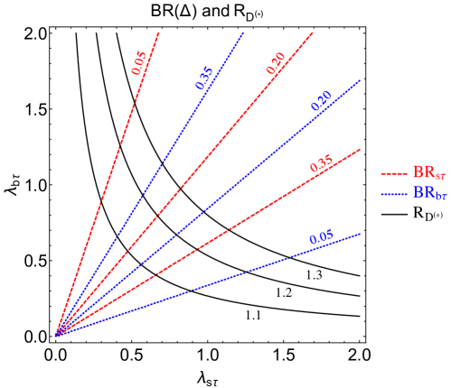
Figure 1:   A comparison of contours of $\mathcal{R}_{D^{(\star)}}$, normalised to their SM values, and $\text{BR}\left(\Delta\rightarrow s\tau(b\tau)\right)$ in black and red (blue), respectively.

Comparing (16) to (17), one sees that the former constrains a product of LQ couplings, whereas the latter constrains a ratio. Hence, in the event of a discovery being made at the LHC, we note that combining this information would allow for a direct experimental probe at the level of individual couplings in the overall flavour matrices $\lambda_{dl,u\nu}$. We show this qualitatively in Fig. 1, given the approximations in (16)-(17), where we have presented experimentally relevant values of $\mathcal{R}_{D^{(\star)}}$ and various values of $\text{BR}\left(\Delta\rightarrow s\tau(b\tau)\right)$, in the context of the $\tau$-isolation model $\lambda^{[\tau]}_{dl}$. Note that in this model SU(2) rotations lead to non-negligible contributions from the $u-\nu$ sector, cf. Fig. 3.

In order to fully determine the parameters of the SMFL, also the LQ mass $M_{\Delta}$ and the LQ coupling parameters $k_{s},k_{Y}$ need to be measured. $k_{s}$ and $M_{\Delta}$ can be accessed through the LQ pair-production cross-section in $pp$ collisions and the invariant mass of the LQ decay products. The parameter $k_{Y}$ is more difficult to access, as it is responsible for the coupling strength of the LQ to the photon and, to a lesser extent, to the $Z$ boson.

3 Precision Constraints and Global Likelihoods

Our goal is to now provide a robust examination of the SMFL parameter space favoured by present-day experiment, and our primary tool in this effort will be smelli [69], an open-source python package which builds upon the flavio [90] and Wilson [91] programs. The goal of flavio is to enable the automated calculation of flavoured processes in terms of dimension-six Wilson coefficients $C$ of the SM effective field theory (SMEFT, valid above the EW scale) or the WET (valid below the EW scale). This package includes a large library of experimental measurements in the flavour and EW sectors. In addition, Wilson computes the renormalization group evolution (RGE) of SMEFT operators, their matching onto the WET at relevant scales, and the further RGE running of WET operators to hadronic scales that are (often) of interest in flavour physics. Augmenting these capabilities, smelli computes a global likelihood function in the space of SMEFT coefficients, i.e. the object

$$L_{\text{SMEFT}}(\vec{C})=\prod_{i}L_{\text{exp}}\left(\vec{O}^{\text{exp}}_{i},\vec{O}^{\text{th}}_{i}\left(\vec{C},\vec{\theta}\right)\right)\times L_{\theta}\left(\vec{\theta}\right)\,.$$ (18)

Here $L_{\text{exp}}$ are likelihood distribution functions which depend on independent experimental measurements $\vec{O}^{\text{exp}}_{i}$ with associated theory predictions $\vec{O}^{\text{th}}_{i}$, which are themselves functions of the Wilson coefficients $\vec{C}$ and additional model-independent phenomenological parameters $\theta$ (e.g. form factors and decay constants). Then $L_{\theta}$ accounts for any experimental or theoretical constraints on these nuisance parameters. Note however that the actual smelli implementation of (18) relies on a ‘nuisance-free’ approximation to the total global likelihood function, which effectively ‘integrates out’ the theoretical errors associated to $\theta$, treating them as additional experimental uncertainties. This is achieved by a factorization of $L_{\text{SMEFT}}$ into likelihoods for observables that a) have negligible theoretical vs. experimental uncertainty or b) that have reliably Gaussian theory and experimental uncertainties, and where the former only weakly depends on $\vec{C}$ and $\vec{\theta}$. While care must be taken for certain observables (e.g. CKM angles) that do not necessarily respect these assumptions, they are reliable and frequently employed (see e.g. [92, 93, 94, 95]) for the analyses we are attempting here. Finally, smelli also includes the one-loop RGE that mix flavour structures in the SMEFT, and which are required for a consistent matching to the WET, where QCD and QED renormalization is flavour-blind [96, 97, 98, 99, 100, 101, 102]. This matching and associated RGE is performed automatically in smelli, allowing coherent comparisons to low-energy experimental data given a UV new physics scale $\Lambda$. For a more complete description of smelli functionality, its built-in assumptions, and an exhaustive list of observables included in its likelihoods, see [69] and the documentation at https://github.com/smelli/smelli.

3.1 Matching the Vector Leptoquark Singlet

In order to perform a ${\tt{smelli}}$ analysis for our SMFL, we first recall the tree-level SMEFT matching onto the LL operators of the $\Delta^{\mu}$ vector LQ singlet given in (7). When computed at the new physics scale $\Lambda=M_{\Delta}$ it yields (see e.g. [103]):

$$\left[C_{LQ}^{(1)}\right]_{ijkl}=\left[C_{LQ}^{(3)}\right]_{ijkl}=-\frac{\lambda_{LQ}^{kj}\,\lambda_{LQ}^{li\star}}{2M_{\Delta}^{2}}\,,$$ (19)

which are the Wilson coefficients of the dimension-six four-fermion SMEFT operators given by

$$\left[\mathcal{O}^{(1)}_{LQ}\right]_{ijkl}=\left(\overline{L}_{i}\gamma_{\mu}L_{j}\right)\left(\overline{Q}_{k}\gamma_{\mu}Q_{l}\right),\,\,\,\,\,\,\,\,\,\,\left[\mathcal{O}^{(3)}_{LQ}\right]_{ijkl}=\left(\overline{L}_{i}\gamma_{\mu}\tau^{I}L_{j}\right)\left(\overline{Q}_{k}\gamma_{\mu}\tau^{I}Q_{l}\right).$$ (20)

In addition to this tree-level matching, we follow [37] and include additional one-loop matching contributions to quark dipole operators in the SMEFT, which can generate the known [104] vector LQ singlet matching contributions to electric and chromomagnetic dipole operators in the low-energy WET. The relevant dimension-six SMEFT operators are

$$\left[\mathcal{O}_{dB}\right]_{ij}=\left(\overline{Q}_{i}\sigma^{\mu\nu}d_{j}\right)\phi\,B_{\mu\nu}\,,\,\,\,\,\,\,\left[\mathcal{O}_{dW}\right]_{ij}=\left(\overline{Q}_{i}\sigma^{\mu\nu}d_{j}\right)\tau^{I}\phi\,W^{I}_{\mu\nu}\,,\,\,\,\,\,\,\left[\mathcal{O}_{dG}\right]_{ij}=\left(\overline{Q}_{i}\sigma^{\mu\nu}T^{A}d_{j}\right)\phi\,G^{A}_{\mu\nu}\,,$$

which are catalogued alongside all remaining independent dimension-six operators in [105]. Note that in smelli the Warsaw basis of [105] (the flavio basis of [90]) is the default basis when obtaining likelihoods in the SMEFT (WET). Again computing the relevant matching at $\Lambda=M_{\Delta}$, one finds [37]

$$\left[C_{dW}\right]_{23} =\frac{Y_{b}}{6}\frac{g}{16\pi^{2}}\frac{\lambda_{LQ}^{2i}\lambda_{LQ}^{3i\star}}{M_{\Delta}^{2}}\,,\,\,\,\,\,\,\,\,\left[C_{dB}\right]_{23}=-\frac{4Y_{b}}{9}\frac{g^{\prime}}{16\pi^{2}}\frac{\lambda_{LQ}^{2i}\lambda_{LQ}^{3i\star}}{M_{\Delta}^{2}}\,,\,\,\,\,\,\,\,\,\left[C_{dG}\right]_{23}=-\frac{5Y_{b}}{12}\frac{g_{s}}{16\pi^{2}}\frac{\lambda_{LQ}^{2i}\lambda_{LQ}^{3i\star}}{M_{\Delta}^{2}}\,$$

$$\left[C_{dW}\right]_{32} =\frac{Y_{s}}{6}\frac{g}{16\pi^{2}}\frac{\lambda_{LQ}^{3i}\lambda_{LQ}^{2i\star}}{M_{\Delta}^{2}}\,,\,\,\,\,\,\,\,\,\left[C_{dB}\right]_{32}=-\frac{4Y_{s}}{9}\frac{g^{\prime}}{16\pi^{2}}\frac{\lambda_{LQ}^{3i}\lambda_{LQ}^{2i\star}}{M_{\Delta}^{2}}\,,\,\,\,\,\,\,\,\,\left[C_{dG}\right]_{32}=-\frac{5Y_{s}}{12}\frac{g_{s}}{16\pi^{2}}\frac{\lambda_{LQ}^{3i}\lambda_{LQ}^{2i\star}}{M_{\Delta}^{2}}\,.$$

Here the lepton index $i$ is summed over. In addition to the Lagrangian conventions discussed above Section 2.2, these were also computed in the limit of a diagonal down-quark Yukawa matrix, with $Y_{s,b}$ the respective Yukawa couplings to strange and bottom quarks. Note that, as mentioned above, one expects logarithmic divergences to appear in dipole processes in the ‘minimal’ coupling scenario where $k=1$ in (4) [70, 24], and therefore the operators in (LABEL:eq:oneloopC) may not be induced in a sensible UV matching with this parameter choice. It is also clear that, when $k=1$, triple-vector couplings between $\Delta-\Delta-B/G$ are not present at tree level, and therefore the one-loop diagram leading to non-zero $C_{dG}$ (e.g.) is not present. Regardless, we note that our analysis in Section 4 is largely insensitive to these UV details, as we have found that turning off all of the dipole operators in (LABEL:eq:oneloopC) only results in a roughly 1$\%$ correction to the best-fit ratio of $\lambda_{s\tau}/\lambda_{b\tau}$ when $M_{\Delta}=1$ TeV (e.g.). In what follows we therefore show fit results in the ‘full’ $k=0$ scenario.

Finally, we recall that as with other similar studies, we have chosen to set the RR couplings $x^{RR}$ and $x^{\overline{RR}}$ in (7) to zero. As can be deduced from model-independent EFT fits (see e. g. [106, 107, 37, 108, 109, 110]) and as will be seen explicitly below, these RH couplings are not necessary in minimal explanations of the observed LFU anomalies, and it has been further shown [59] that exclusion limits on $M_{\Delta}$ strengthen when $x^{RR}\neq 0$. Hence (19)-(LABEL:eq:oneloopC) represent the complete set of relevant SMEFT Wilson coefficients implemented in our smelli analysis.

3.2 Scanning the Vector Leptoquark Singlet

Given (19)-(LABEL:eq:oneloopC), one is in a position to scan over the SMFL couplings $\lambda_{dl}$ and allow smelli to compute likelihoods at each phase-space point. One can collect this information as a function of $\lambda_{dl}$ and determine the experimentally favoured space of couplings for a given SMFL pattern/model, as well as the observables which contribute the most significant pulls.


Specifically, in performing our scans we

1. take the LQ couplings $\lambda_{dl}$ to be real. As will be seen, there is ample parameter space of interest even without additional complex degrees of freedom.

2. build an array of $\{\lambda_{sl},\lambda_{bl}\}$ by dividing the phase space in either dimension by a predefined set of intervals. We then calculate the Wilson coefficients in (19)-(LABEL:eq:oneloopC) for all points on this grid.

3. perform a global likelihood analysis using smelli v2.3.2 at each parameter point on the $\lambda_{dl}$ grid. This is performed by calling smelli.GlobalLikelihood(), which we also modify using the custom_likelihoods attribute. This latter functionality allows us to define custom sets of observables contributing to a likelihood computation.

4. collect all likelihoods computed and determine the values associated to the minimum $\Delta\chi^{2}$ for a given pattern (and a given set of observables). We do so by calling the log_likelihood_global() method, which returns $\Delta\log L=-\Delta\chi^{2}/2$, where $\Delta\chi^{2}$ is the BSM $\chi^{2}$ minus its SM value. We use this to then compute 1$\sigma$ and 2$\sigma$ likelihood contours about the $\Delta\chi^{2}$ minimum.

5. in order to determine the relative pull of any given set of observables, we also use the log_likelihood_dict() method, which returns the dictionary of all contributions to $\Delta\log L$ from the individual products in (the smelli implementation of) (18). Note that in addition to the classes of observables already segregated in smelli through the inclusion of separate internal YAML files, any of the custom_likelihoods we defined ourselves will also be given as independent contributions.

We now report the results of these scans for SMFL patterns of distinct phenomenological interest: the lepton isolation patterns $\lambda_{dl}^{[e,\mu,\tau]}$. We also report the relative pull of $\mathcal{R}_{K^{(*)},D^{(*)}}$ (at the global $\Delta\log L$ maximum), which are especially interesting due to their present deviations from SM predictions.

SMFL	$M_{\Delta}$	Best Fit $\left(\lambda_{sl},\lambda_{bl}\right)$	$\Delta\log L|_{\mathcal{R}_{D^{(\star)}}}$	$\Delta\log L|_{\mathcal{R}_{K^{(\star)}}}$	$\Delta\log L|_{\text{Global}}$
$\lambda_{dl}^{[\tau]}$	2 TeV	$\left(0.64,0.72\right)$	12.638	N.A.	18.457
	1 TeV	$\left(0.30,0.38\right)$	12.622		17.970
$\lambda_{dl}^{[\mu]}$	2 TeV	$\left(0.147,-0.021\right)$	0.107	6.535	20.648
	1 TeV	$\left(0.078,-0.01\right)$	0.107	6.469	20.812
$\lambda_{dl}^{[e]}$	2 TeV	$\left(0.016,0.172\right)$	-$\mathcal{O}(10^{-2})$	7.306	8.222
	1 TeV	$\left(0.006,0.114\right)$	-$\mathcal{O}(10^{-2})$	7.302	8.224

Table 1: Results from the $M_{\Delta}=\{1,2\}$ TeV two-parameter likelihood ($\Delta\log L=-\Delta\chi^{2}/2$) scans of Section 3.2, including the individual contributions of the (potentially) anomalous observables $\mathcal{R}_{K^{(\star)},D^{(\star)}}$. Column 3 gives the best-fit values of $\left(\lambda_{sl},\lambda_{bl}\right)$, corresponding to the global likelihood maximum of the scans, found in column 6, which consider all available data in smelli. Columns 4-5 then give the individual contributions of $\mathcal{R}_{K^{(\star)},D^{(\star)}}$ to this likelihood (again at the best-fit coordinates). See the text and Figure 2 for more details.

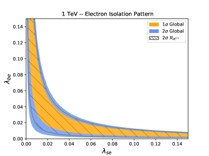
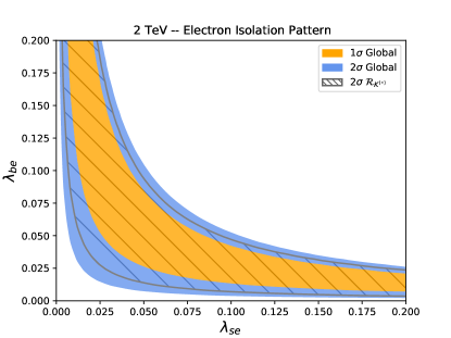
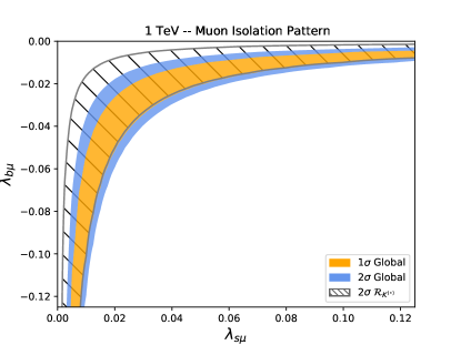
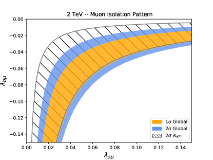
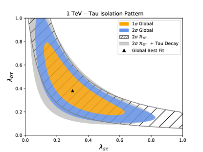
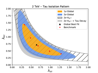
Figure 2:   Top Left: Likelihood contours for the two-parameter $e$-isolation pattern $\lambda_{dl}^{[e]}$ at $M_{\Delta}=1$ TeV, including $2\sigma$ contours from $\mathcal{R}_{K^{(\star)}}$ constraints alone (hatched region), as well as global $1\sigma$ (orange region) and $2\sigma$ (blue region) preferred contours considering all data available to smelli. Top Right: The same, but for $M_{\Delta}=2$ TeV. Middle Row: The same, but for the $\mu$-isolation pattern $\lambda_{dl}^{[\mu]}$. Bottom Row: The same, but for the $\tau$-isolation pattern $\lambda_{dl}^{[\tau]}$, and including $2\sigma$ contours from $\mathcal{R}_{D^{(\star)}}$ constraints alone (hatched region), and $\mathcal{R}_{D^{(\star)}}+\tau$ decay modes (gray region). Here the global best-fit (black, triangular) and benchmark (red, circular) points in $\{\lambda_{s\tau},\lambda_{b\tau}\}$ we obtained from our scan are also shown.

Electron and Muon Isolation Patterns

We first investigate $\lambda_{dl}^{[e,\mu]}$ from (12), the e- and $\mu$-isolation patterns, where the results of the smelli scans we performed as described above are given in the top (middle) panels of Figure 2 for the electron (muon) patterns, as well as numerically in Table 1. One observes in Figure 2 that a broad range of couplings is allowed at the 1$\sigma$ and 2$\sigma$ confidence level, considering all available data, and that the potentially anomalous measurement of $\mathcal{R}_{K^{(\star)}}$ is well-described in these models. Indeed, the overall shape of the global parameter space preferred largely follows that preferred by $\mathcal{R}_{K^{(\star)}}$ alone. Note that the 2021 measurement of $\mathcal{R}_{K}$ [48] increased the tension with the SM, implying a stronger preference for non-zero LQ couplings $\lambda_{qe}$ and $\lambda_{q\mu}$ (with $q=b,s$). The additional pull to non-zero couplings in the $\mu$-isolation pattern originates in the so-called $b\to s\mu^{+}\mu^{-}$ anomalies observed in the decays $B\to K^{*}\mu^{+}\mu^{-}$, $B_{s}\to\phi\mu^{+}\mu^{-}$ etc. that can not be addressed in the electron-isolation pattern. In the latter case, non-zero couplings have received further support from the recent update of the $B^{0}\to K^{*0}\mu^{+}\mu^{-}$ angular analysis [131], the newly measured $B^{+}\to K^{*+}\mu^{+}\mu^{-}$ angular observables [132], and the recent experimental update of the $B_{s}\to\phi\mu^{+}\mu^{-}$ branching ratio [133]. We refer the reader to [46] for further details on the implications of these measurements. Additionally, as seen in Table 1, the global best-fit value is also favoured over SM couplings alone as it slightly softens the charged-current LFU anomaly $\mathcal{R}_{D^{(\star)}}$, at least for the $\mu-$isolation pattern. When considering only $\mathcal{R}_{D^{(\star)}}$ data, better likelihoods can be obtained in the parameter space scanned. $\lambda_{dl}^{[\mu]}$’s ability to resolve LFU anomalies whilst generating a distinct collider phenomenology has been known for some time (see e.g. [111, 112]).

As a final note, we have observed that the overall $-\Delta\chi^{2}/2$ likelihood distributions for both $\lambda_{dl}^{[e,\mu]}$ are somewhat flat, in that multiple points spanning a broad domain in the two-dimensional contours presented fall very close to the likelihood found for the global best-fit point. For example, we can identify a number of parameter space points whose likelihoods are within a percent (or less) of the global maximum, but whose coordinates are a factor of 2 (or more) away from those presented in Table 1. We found this behavior for $\lambda_{dl}^{[e,\mu]}$ at both $M_{\Delta}=\{1,2\}$ TeV, and it is for this reason that we do not find it instructive to plot a ‘global’ best-fit point in Figure 2, but instead give this information in Table 1, to illustrate the overall quality of the fits.

Tau Isolation Pattern

We next investigate $\lambda_{dl}^{[\tau]}$ from (12), the $\tau$-isolation pattern. This texture has been studied before in the context of a toy vector singlet LQ model [37] (although without the SMFL symmetry-based motivation for its flavour structure), and here we update those results given improved experimental and theoretical developments over the last years.

Using the algorithm described in Section 3, we produce the bottom panels in Figure 2. The graphics illustrate the contours contributing to the global likelihood coming from the ratio observables $\mathcal{R}_{D^{(\star)}}$ (hatched region), those from a custom fit combining both $\mathcal{R}_{D^{(\star)}}$ and the leptonic $\tau$-decay modes $\text{BR}\left(\tau^{-}\rightarrow l^{-}\nu\bar{\nu}\right)$ with $l=e,\mu$, $\text{BR}\left(\tau^{+}\rightarrow K^{+}\bar{\nu}\right)$, and $\text{BR}\left(\tau^{+}\rightarrow\pi^{+}\bar{\nu}\right)$ (gray region), and finally the global $1\sigma$ (orange region) and $2\sigma$ (blue region) preferred contours upon considering all experimental datasets in smelli. Note that leptonic $\tau$ decays and $\mathcal{R}_{D^{(\star)}}$ were identified as dominant contributors to the overall likelihoods for $\lambda_{dl}^{[\tau]}$ in [37], and we confirm that observation in our analysis. We give these at $M_{\Delta}=\{1,2\}$ TeV (left and right panels, respectively), and the best-fit $\left(\lambda_{s\tau},\lambda_{b\tau}\right)$ values are shown in black, where the global likelihood maxima of our scans are realized. The numerical values of these coordinates as well as the maximum $\Delta\log L$ is again given in Table 1. For the 2 TeV contours we also plot ‘benchmark points’ in red that we will use in the upcoming collider analysis of Section 4.

Finally, we observe from Table 1 that the overall global likelihood for $\lambda_{dl}^{[\tau]}$ is significantly larger than that found when considering $\mathcal{R}_{D^{(\star)}}$ alone. This effect has been observed before, and can be traced back to gauge-induced one-loop renormalization group mixing that generates a lepton-universal contribution to the semi-leptonic operators of (20) (above and below the EW scale), from the non-universal, $\tau$-specific semi-leptonic operator matched at tree-level (cf. (19) for the $\lambda_{dl}^{[\tau]}$ SMFL)— see e.g. the discussion in [37, 104]. The operator mixing therefore makes this $\tau$-isolation pattern sensitive to other semileptonic processes, e.g. $B\longrightarrow K^{(\star)}\ell\ell$ branching ratios and angular observables, measurements of which are considered in the global likelihood.

Summary

In conclusion, it is clear that the $\mu$- and the $\tau$-isolation patterns both provide excellent fits to the available data across a broad range of parameter space, and are able to solve the LFU anomalies $\mathcal{R}_{K^{(*)}}$ and $\mathcal{R}_{D^{(*)}}$, respectively. While the electron isolation pattern can also successfully address $\mathcal{R}_{K^{(*)}}$, it falls short of explaining the related anomalies in $b\to s\mu^{+}\mu^{-}$ transitions, and is hence less motivated from a phenomenological perspective.

In what follows we will further pursue the analysis of the $\tau$-isolation pattern and study its LHC signatures. A high-$p_{T}$ study of this scenario is particularly motivated, since we have seen that large LQ couplings are required by the global fit. In turn this precludes the possibility of evading direct searches by simply raising the LQ mass $M_{\Delta}$ beyond the reach of the LHC.

4 Recasting LHC Exclusion Limits

In this Section we consider existing direct searches published by ATLAS [114] and reinterpret them in the context of our well motivated $\tau-$isolation scenario. In particular, both second- and third-generation quarks can be involved in the LQ decay. Assuming only left-handed couplings, and neglecting the fermion masses as well as CKM rotations, the different branching ratios exhibit the following structure

$$\text{BR}_{\Delta}^{3^{\text{rd}}}=\text{BR}(\Delta\rightarrow b\tau)\simeq\text{BR}(\Delta\rightarrow t\nu),$$ (22)

$$\text{BR}_{\Delta}^{2^{\text{nd}}}=\text{BR}(\Delta\rightarrow s\tau)\simeq\text{BR}(\Delta\rightarrow c\nu)\simeq 0.5-\text{BR}_{\Delta}^{3^{\text{rd}}}\,,$$ (23)

where $\text{BR}_{\Delta}^{2^{\text{nd}}}$ ($\text{BR}_{\Delta}^{3^{\text{rd}}}$ ) corresponds to the decay into the second (third) down-type quark. This structure holds very well as shown in Figure 3 where the CKM and fermion mass effects have been taken into account with a 2 TeV mass for the LQ. Using (17) we obtain the following relation for the branching ratio as a function of the couplings:

$$\text{BR}_{\Delta}^{3^{\text{rd}}}\simeq\frac{1}{2}\frac{\lambda_{b\tau}^{2}}{\lambda_{b\tau}^{2}+\lambda_{s\tau}^{2}}.$$ (24)

$\lambda_{dl}^{[\tau]}$ Benchmark Points BPi ($\lambda_{s\tau},\,\lambda_{b\tau}$) BP1 (1.29, 0.4) BP2 ( 0.98, 0.49) BP3 (0.68, 0.68) BP4 (0.48, 0.96) BP5 (0.32, 1.43)

Table 2:   $\text{BR}(\Delta(\Delta)\rightarrow QL(QL))$ for 2 TeV LQ Benchmark Points from the $\lambda_{dl}^{[\tau]}$ scan of Section 3. All asymmetric decay BR have an additional $\times 2$ factor because of permutation.

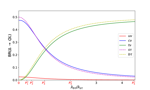
Figure 3: 2 TeV LQ branching ratios into quarks and leptons for the $\tau-$ isolation pattern. The channel magnitudes only depend on the ratio of the couplings. The non-vanishing $u-\nu$ contribution appears due to CKM rotations from $\lambda_{d\ell}\rightarrow\lambda_{u\nu}$. The other channels are (almost) exactly vanishing in the context of the $\tau-$isolation pattern. We have highlighted in red the position of the different benchmark points shown in Figure 2. Note that $P_{2}^{\tau}$, $P_{3}^{\tau}$ and $P_{4}^{\tau}$ have $\lambda_{b\tau}/\lambda_{s\tau}$ values of 0.5, 1 and 2, respectively.

As an example, we selected five benchmark points labelled $P_{i}^{\tau}$ across the $1\sigma$ fit region of Figure 2. These scenarios have distinct decay channel magnitudes and are therefore rather illustrative for collider considerations. All information regarding these benchmark points is gathered in Table 2.

The procedure regarding our collider analysis is as follows: we first consider the mixed search $\Delta\rightarrow b\tau/t\nu$ investigated in [114] where we adapt to match the extra opened second-generation quark channel. We then complete the analysis by confronting our model with the implemented LHC searches in CheckMATE [115, 116]. Of particular interest would be the jets and missing energy searches, since the channel involving jets and neutrinos remains stable around 50% as discussed in (23). We present results for the two extreme cases for the pair production cross-section: $k=0$ and $k=1$, for which the values are given together with the scalar leptoquark one for comparison in Fig. 4.

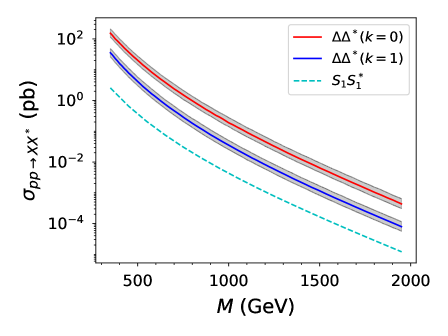
Figure 4: Pair production cross-section for different LQ models. For the vector LQ $\Delta$ we present results for both the $k=0$ and $k=1$ scenarios studied in the text. Uncertainties are calculated for the vector leptoquark model by varying the scale in MadGraph5_aMC@NLO  2.8.2 from 0.5 to 2, with respect to the central default value, see main text for details. The scalar model ($S_{1}$) is presented as an illustration, being the benchmark model employed in most of the ATLAS and CMS studies.

In this section we compute leading-order cross sections and generate parton level events with the help of MadGraph5_aMC@NLO  2.8.2 using an in-house implementation in Feynrules [118, 119] of the Lagrangian from Section 2.1. The NNPDF30_lo_as_0118 [120] set of parton distribution functions (PDF) is employed, which we handle through LHAPDF [121]. The factorization and renormalization scales are set on an event-by-event basis by MadGraph5_aMC@NLO, setting the parameters dynamical_scale_choice and scalefact to -1 and 1.0, respectively. We have verified that varying the scalefact parameter by a factor of two (to 2.0 and 0.5) impacts the cross-section by -30 % and +40 %, respectively. Moreover, this variation is almost independent of the leptoquark mass (scanning in the 0.3-2 TeV range). We have neglected diagrams including a $t$-channel lepton exchange as their contribution is sub-leading with respect to the scale variation . The technical details for the showering and detector simulation of the parton level events (employed as CheckMATE input) are described in Section 4.2.

4.1 Reinterpretation of the Mixed $b\tau\,t\nu$ Search

Several searches at the LHC by the ATLAS [123, 114] and CMS [124, 125, 126] collaborations explicitly target up-type vector LQs with $b\tau$ and $t\nu$ final states. Among those, ATLAS in [114] (CMS in [126]) considers for the first time the possibility of a $b\tau t\nu$ final state (originally pointed out in  [127] and scrutinized in [128, 122]), where each LQ decayed in a different channel. We informally refer to this as the “mixed” channel. Moreover, for the specific case where $\text{BR}(\Delta\rightarrow b\tau)$ and $\text{BR}(\Delta\rightarrow t\nu)$ are approximately equal, the study of reference [114] provides the most stringent constraints, and hence, among the whole suite of LQ studies, we focus on the reinterpretation of this specific final state.

The ATLAS study [114] considers LQ decays exclusively to third-generation quarks, and hence the branching ratios into $t\nu$ and $b\tau$ add up to unity. However, in more generic setups additional decay channels can be opened. Following the strategy proposed in [122] we reinterpreted the search in this more generic framework, for our vector LQ model. Here we briefly sketch the basics of our procedure, and refer the reader to reference [122] for details. Note that in the following we re-interpret the ATLAS search and not the same final state CMS one [126] since the ATLAS search is more sensitive for vector LQs in the parameter space of interest.

The number of events in a signal region is proportional to the pair production cross section $\sigma(pp\to\Delta\Delta)\equiv\sigma$, to the branching ratios for $\Delta\to b\tau$ and $\Delta\to t\nu$ and to the acceptance $A$ and efficiency $\epsilon$ in the signal regions. The latter two functions are reported in the auxiliary material of  [114] for several LQ scenarios, including the minimal coupling ($k=1$) and Yang-Mills ($k=0$) incarnations of our $\Delta_{\mu}$ vector case, as a function of the mass and the branching ratio into $b\tau$, where it is assumed that the $\Delta\to t\nu$ channel is the only other channel open. Since this assumption does not hold in general for our benchmark points, the crucial point discussed in Section 3.2.2 of reference [122] is that $A(M,x)$ should be instead $A(M,x^{\prime})$ where $x=\text{BR}(\Delta\rightarrow b\tau)$ and $x^{\prime}=\text{BR}(\Delta\rightarrow b\tau)/(\text{BR}(\Delta\rightarrow b\tau)+\text{BR}(\Delta\rightarrow t\nu))$; and analogously for the $\epsilon$ functions. The reason behind this choice is the fact that the mixed search should only depend on the relative weight of the $b\tau$ to the $t\nu$ final state. In our case, given by eq. (23), we see that $x^{\prime}\approx 0.5$. We do not attempt to reproduce the ATLAS counts in each signal region, since ultimately the final exclusion from ATLAS comes from a combination of signal regions which we can not perform without knowing the relevant correlations, which are regrettably not publicly available. Instead, we will exploit the fact that the ATLAS paper explicitly excludes a mass of 1.50 TeV (1.77 TeV) for $x=0.5$ and $k=1$ ($k=0$), and we will simply request to have the same events for the exclusion as those obtained for a mass of 1.50 TeV (1.77 TeV) and $\text{BR}_{\Delta}^{3^{\text{rd}}}=0.5$. Then the excluded value (at $95\%$ C.L.) of $\text{BR}_{\Delta}^{3^{\text{rd}}}$ for a given mass $M$ is given approximately, for the $k=1$ case, by

$$(\text{BR}_{\Delta}^{3^{\text{rd}}})^{\rm 95}=0.5\Biggl{(}\frac{\sigma(1.5{\rm TeV})A(1.5{\rm TeV},0.5)\epsilon(1.5{\rm TeV},0.5)}{\sigma(M)A(M,0.5)\epsilon(M,0.5)}\Biggr{)}\,.$$ (25)

While the numerical impact of abandoning this approximation is small, along this work we have nonetheless evaluated the corresponding functions at the corresponding value of $x$, including the finite top mass effects in the $\Delta$ branching ratios.

Following the procedure described above, and using our results for the production cross-section as a function of the mass, given in Figure 4, it is possible to extend the exclusion given by ATLAS to include the effect of the additional open channels by varying $\text{BR}_{\Delta}^{3^{\text{rd}}}$ instead, which can be matched to the ratio $\lambda_{b\tau}/\lambda_{s\tau}$. The result is presented in Figure 5. We observe that, as expected, the excluded mass drops significantly as the branching ratio into the third generation quarks decreases. The two extreme cases from the best fits presented in Section 3.2 are reached for BP1 and BP5, for which we exclude masses close to 600 GeV (900 GeV) and 1500 GeV (1750 GeV) for $k=1$ ($k=0$), respectively.

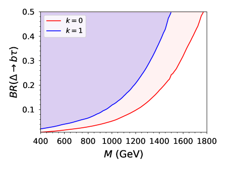
Figure 5: Reinterpretation from [114]. The main assumptions are $\text{BR}(\Delta\rightarrow b\tau)=\text{BR}(\Delta\rightarrow t\nu)$ and that the opened second generation decay is invisible to the analysis, and hence only affects the fiducial cross-section $2\times\sigma(pp\rightarrow\Delta\Delta^{*})\times(\text{BR}_{\Delta}^{3^{\text{rd}}})^{2}$.

4.2 CheckMATE Exclusion Limits

As discussed previously, we expect searches involving multi-jets and missing energy to complete the exclusion limits provided by the reinterpretation of the mixed channel. Indeed, at parton level, the branching ratio of the LQ decay channel involving a neutrino ($t\nu+c\nu$) remains stable around 50% across the coupling parameter space as only the left-handed coupling is present. Decay channels involving either one or two neutrinos will therefore be probed by these searches.

We perform a parameter scan in the plane $\left(M,\lambda_{b\tau}/\lambda_{s\tau}\right)$ as only the coupling ratio has an impact on the collider phenomenology. For each parameter point, we generate 10,000 events at parton level using MadGraph 5 2.8.2 [117] which are then passed through Pythia 8 [140] for showering and hadronization. Finally, Delphes 3.4.2 [136] and its official ATLAS card are used for fast detector simulation. The full parameter scan is composed of two grids for the two cases $k=0,1$. For $k=0$ (resp. $k=1$), the grid is composed of twelve points $\in[0.31,3.06]$ (resp. plus two extra points at 0.12, 0.41 needed for better precision) along the $\lambda_{b\tau}/\lambda_{s\tau}$ axis and five (resp. six) points $\in[1675,1875]$ GeV (resp. $\in[1000,1250]$ GeV) along the $M$ axis. Using CheckMATE v 2.0.34 [116] , we compute for each point in the parameter space the $r_{95}$ value [139]. This quantity is defined for a given signal region, in a specific experimental analysis, as the ratio between a) the number of predicted signal events and b) the 95% C.L. exclusion limit provided by the collaboration. Therefore, a point in parameter space is considered excluded if in any of the channels $r_{95}>1$. Furthermore, CheckMate provides together with the $r_{95}$ value, the corresponding most sensitive channel. Using the interpolation function interp1d provided by the scipy python package, we obtained the $95\%$ C.L. exclusion limit from CheckMATE reached for $r_{95}=1$. The results are shown in Fig. 6 together with the mixed search, adapted to the $\left(M,\lambda_{b\tau}/\lambda_{s\tau}\right)$ plane using the expression for the branching ratios (24).

The exclusion is dominated by analyses that involve large missing energy. In particular, the $nj+\not{E}_{T}$ search released in [134] is responsible for most of the parameter space exclusion. On the other hand, the searches for sleptons in $n\ell+\not{E}_{T}$ or more specifically staus in $n\tau+\not{E}_{T}$ [135] give the dominant contribution for a smaller set of points. All relevant analyses have a luminosity of 139 fb^-1.

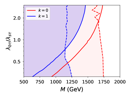
Figure 6: Combined results from CheckMATE $nj+\not{E}_{T}$ and mixed-channel exclusion limits. Solid lines correspond to the mixed channel while the dashed ones are the results from CheckMATE. Note that the y-axis has a base 2 logarithmic scale.

We note that the limits depend only weakly on the coupling ratio with the excluded values for $k=0$ ($k=1$) close to $\sim 1700$ GeV ($\sim 1150$ GeV), reproducing our expectations from the parton-level consideration where the neutrino channels sum up to $50\%$ independently of the coupling ratio.

Being conservative by assuming that the efficiency of future searches will remain stable and therefore simply rescaling by the luminosity, one can estimate prospects for HL-LHC for 3000 fb^-1, which should exclude masses of order 1400 GeV (2000 GeV) for $k=1$ ($k=0$). However, due to the improvement of the analysis techniques (for example in [130] compared to [129]), one can be more optimistic and expect even higher masses to be reached. We then see that both classes of studies (searches for LQs and missing energy searches) complement each other and that enhancing the sensitivity of these studies is of crucial importance towards shedding light on the mechanism(s) behind the flavour anomalies.

5 Summary and Outlook

We have studied the phenomenological consequences of a subset of Simplified Models of Flavourful Leptoquarks [34, 35, 36] that only couple to a single generation of charged leptons, with a central focus on the $\left({\bf{3}},{\bf{1}},2/3\right)$ vector leptoquark $\Delta_{\mu}$ coupling quarks to $\tau$ leptons. Lepton isolation patterns/models are readily motivated by ultraviolet flavour-symmetry breaking, and are amongst the most minimal scenarios that can explain experimental anomalies in the lepton-flavour-universality observables $\mathcal{R}_{D^{(\star)},K^{(\star)}}$, depending on the actual tree-level lepton couplings allowed. We reviewed their theoretical motivation and used smelli [69] to scan over the global parameter space favoured by low-energy flavour data when couplings to electrons, muons, or taus are permitted. This analysis revealed that all three patterns are favoured over SM physics alone, and we presented $1\sigma$ and $2\sigma$ global likelihood contours in the two-parameter spaces of (12), along with likelihood contours in the same space, but coming from $\mathcal{R}_{D^{(\star)},K^{(\star)}}$ data alone. Upon focusing on the $\tau-$isolation pattern, we then studied the decay signatures of $\Delta_{\mu}$ at the LHC.

Based on our parameter-space scans, we have defined a series of benchmark points to illustrate the main phenomenological features, where the branching fraction into the third generation ranges from a few percent up to almost 100 %. We have confronted the parameter space of our model with two different classes of LHC searches, namely i) direct searches for leptoquarks and ii) missing energy searches. Given that our setup imposes approximately equal branching ratios into $t\nu$ and $b\tau$, it turns out that the mixed ATLAS search looking for $b\tau t\nu$ provides the strongest constraints among the set of direct leptoquark searches. We carried out the reinterpretation of this search for our vector leptoquark models, where the sensitivity would obviously depend on the branching ratio into the third generation. If no additional channels are open, these searches can constrain a leptoquark mass up to 1500 (1770) GeV for the $k=1$ ($k=0$) scenarios, while if instead the branching fraction into the third generation were to be 5%, these upper limits would be reduced to approximately 700 (1000) GeV. Regarding the missing energy searches, since our setup also imposes that our leptoquark decays 50% of the time in a channel with one neutrino, it is not surprising that the mass reach is pretty insensitive to the third generation branching fraction, being about 1150 (1700) GeV for the $k=1$ ($k=0$) case. The complementarity between both types of searches is interesting.

Last but not least, we would like to point out that it would be desirable to expand the set of direct leptoquark searches to specifically target decays into the second generation. While experimentally challenging, it is clear that since the flavour anomalies are directly related to the second generation, searches including $c$ quarks, e.g. $c\nu c\nu$ or $b\tau c\nu$ would have an important impact on both the discovery and the characterization of leptoquark models. While outside the scope of this work, it would also be desirable to study in similar fashion how future colliders can fully probe the vector leptoquark scenario.

References

- [1] J. P. Lees et al. [BaBar], Phys. Rev. Lett. 109 (2012), 101802 doi:10.1103/PhysRevLett.109.101802 [arXiv:1205.5442 [hep-ex]].
- [2] J. P. Lees et al. [BaBar], Phys. Rev. D 88 (2013) no.7, 072012 doi:10.1103/PhysRevD.88.072012 [arXiv:1303.0571 [hep-ex]].
- [3] M. Huschle et al. [Belle], Phys. Rev. D 92 (2015) no.7, 072014 doi:10.1103/PhysRevD.92.072014 [arXiv:1507.03233 [hep-ex]].
- [4] S. Hirose et al. [Belle], Phys. Rev. Lett. 118 (2017) no.21, 211801 doi:10.1103/PhysRevLett.118.211801 [arXiv:1612.00529 [hep-ex]].
- [5] Y. Sato et al. [Belle], Phys. Rev. D 94 (2016) no.7, 072007 doi:10.1103/PhysRevD.94.072007 [arXiv:1607.07923 [hep-ex]].
- [6] S. Hirose et al. [Belle], Phys. Rev. Lett. 118 (2017) no.21, 211801 doi:10.1103/PhysRevLett.118.211801 [arXiv:1612.00529 [hep-ex]].
- [7] A. Abdesselam et al. [Belle], [arXiv:1904.08794 [hep-ex]].
- [8] R. Aaij et al. [LHCb], Phys. Rev. Lett. 115 (2015) no.11, 111803 [erratum: Phys. Rev. Lett. 115 (2015) no.15, 159901] doi:10.1103/PhysRevLett.115.111803 [arXiv:1506.08614 [hep-ex]].
- [9] R. Aaij et al. [LHCb], Phys. Rev. Lett. 120 (2018) no.17, 171802 doi:10.1103/PhysRevLett.120.171802 [arXiv:1708.08856 [hep-ex]].
- [10] R. Aaij et al. [LHCb], Phys. Rev. D 97 (2018) no.7, 072013 doi:10.1103/PhysRevD.97.072013 [arXiv:1711.02505 [hep-ex]].
- [11] Y. S. Amhis et al. [HFLAV], Eur. Phys. J. C 81 (2021) no.3, 226 doi:10.1140/epjc/s10052-020-8156-7 [arXiv:1909.12524 [hep-ex]].
- [12] A. Crivellin, C. Greub and A. Kokulu, Phys. Rev. D 86 (2012), 054014 doi:10.1103/PhysRevD.86.054014 [arXiv:1206.2634 [hep-ph]].
- [13] A. Crivellin, A. Kokulu and C. Greub, Phys. Rev. D 87 (2013) no.9, 094031 doi:10.1103/PhysRevD.87.094031 [arXiv:1303.5877 [hep-ph]].
- [14] A. Celis, M. Jung, X. Q. Li and A. Pich, JHEP 01 (2013), 054 doi:10.1007/JHEP01(2013)054 [arXiv:1210.8443 [hep-ph]].
- [15] P. Ko, Y. Omura and C. Yu, JHEP 03 (2013), 151 doi:10.1007/JHEP03(2013)151 [arXiv:1212.4607 [hep-ph]].
- [16] A. Crivellin, J. Heeck and P. Stoffer, Phys. Rev. Lett. 116 (2016) no.8, 081801 doi:10.1103/PhysRevLett.116.081801 [arXiv:1507.07567 [hep-ph]].
- [17] X. G. He and G. Valencia, Phys. Rev. D 87 (2013) no.1, 014014 doi:10.1103/PhysRevD.87.014014 [arXiv:1211.0348 [hep-ph]].
- [18] A. Greljo, G. Isidori and D. Marzocca, JHEP 07 (2015), 142 doi:10.1007/JHEP07(2015)142 [arXiv:1506.01705 [hep-ph]].
- [19] S. M. Boucenna, A. Celis, J. Fuentes-Martin, A. Vicente and J. Virto, Phys. Lett. B 760 (2016), 214-219 doi:10.1016/j.physletb.2016.06.067 [arXiv:1604.03088 [hep-ph]].
- [20] X. G. He and G. Valencia, Phys. Lett. B 779 (2018), 52-57 doi:10.1016/j.physletb.2018.01.073 [arXiv:1711.09525 [hep-ph]].
- [21] R. Alonso, B. Grinstein and J. Martin Camalich, JHEP 10 (2015), 184 doi:10.1007/JHEP10(2015)184 [arXiv:1505.05164 [hep-ph]].
- [22] L. Calibbi, A. Crivellin and T. Ota, Phys. Rev. Lett. 115 (2015), 181801 doi:10.1103/PhysRevLett.115.181801 [arXiv:1506.02661 [hep-ph]].
- [23] S. Fajfer and N. Košnik, Phys. Lett. B 755 (2016), 270-274 doi:10.1016/j.physletb.2016.02.018 [arXiv:1511.06024 [hep-ph]].
- [24] R. Barbieri, G. Isidori, A. Pattori and F. Senia, Eur. Phys. J. C 76 (2016) no.2, 67 doi:10.1140/epjc/s10052-016-3905-3 [arXiv:1512.01560 [hep-ph]].
- [25] R. Barbieri, C. W. Murphy and F. Senia, Eur. Phys. J. C 77 (2017) no.1, 8 doi:10.1140/epjc/s10052-016-4578-7 [arXiv:1611.04930 [hep-ph]].
- [26] G. Hiller, D. Loose and K. Schönwald, JHEP 12 (2016), 027 doi:10.1007/JHEP12(2016)027 [arXiv:1609.08895 [hep-ph]].
- [27] N. G. Deshpande and A. Menon, JHEP 01 (2013), 025 doi:10.1007/JHEP01(2013)025 [arXiv:1208.4134 [hep-ph]].
- [28] M. Tanaka and R. Watanabe, Phys. Rev. D 87 (2013) no.3, 034028 doi:10.1103/PhysRevD.87.034028 [arXiv:1212.1878 [hep-ph]].
- [29] Y. Sakaki, M. Tanaka, A. Tayduganov and R. Watanabe, Phys. Rev. D 88 (2013) no.9, 094012 doi:10.1103/PhysRevD.88.094012 [arXiv:1309.0301 [hep-ph]].
- [30] M. Freytsis, Z. Ligeti and J. T. Ruderman, Phys. Rev. D 92 (2015) no.5, 054018 doi:10.1103/PhysRevD.92.054018 [arXiv:1506.08896 [hep-ph]].
- [31] M. Bauer and M. Neubert, Phys. Rev. Lett. 116 (2016) no.14, 141802 doi:10.1103/PhysRevLett.116.141802 [arXiv:1511.01900 [hep-ph]].
- [32] D. Bečirević, S. Fajfer, N. Košnik and O. Sumensari, Phys. Rev. D 94 (2016) no.11, 115021 doi:10.1103/PhysRevD.94.115021 [arXiv:1608.08501 [hep-ph]].
- [33] D. Bečirević, I. Doršner, S. Fajfer, N. Košnik, D. A. Faroughy and O. Sumensari, Phys. Rev. D 98 (2018) no.5, 055003 doi:10.1103/PhysRevD.98.055003 [arXiv:1806.05689 [hep-ph]].
- [34] I. de Medeiros Varzielas and J. Talbert, Eur. Phys. J. C 79 (2019) no.6, 536 doi:10.1140/epjc/s10052-019-7047-2 [arXiv:1901.10484 [hep-ph]].
- [35] J. Bernigaud, I. de Medeiros Varzielas and J. Talbert, JHEP 01 (2020), 194 doi:10.1007/JHEP01(2020)194 [arXiv:1906.11270 [hep-ph]].
- [36] J. Bernigaud, I. de Medeiros Varzielas and J. Talbert, Eur. Phys. J. C 81 (2021) no.1, 65 doi:10.1140/epjc/s10052-021-08882-7 [arXiv:2005.12293 [hep-ph]].
- [37] J. Aebischer, W. Altmannshofer, D. Guadagnoli, M. Reboud, P. Stangl and D. M. Straub, Eur. Phys. J. C 80 (2020) no.3, 252 doi:10.1140/epjc/s10052-020-7817-x [arXiv:1903.10434 [hep-ph]].
- [38] N. Assad, B. Fornal and B. Grinstein, Phys. Lett. B 777 (2018), 324-331 doi:10.1016/j.physletb.2017.12.042 [arXiv:1708.06350 [hep-ph]].
- [39] J. C. Pati and A. Salam, Phys. Rev. D 10 (1974), 275-289 [erratum: Phys. Rev. D 11 (1975), 703-703] doi:10.1103/PhysRevD.10.275
- [40] L. Di Luzio, A. Greljo and M. Nardecchia, Phys. Rev. D 96 (2017) no.11, 115011 doi:10.1103/PhysRevD.96.115011 [arXiv:1708.08450 [hep-ph]].
- [41] L. Calibbi, A. Crivellin and T. Li, Phys. Rev. D 98 (2018) no.11, 115002 doi:10.1103/PhysRevD.98.115002 [arXiv:1709.00692 [hep-ph]].
- [42] M. Bordone, C. Cornella, J. Fuentes-Martin and G. Isidori, Phys. Lett. B 779 (2018), 317-323 doi:10.1016/j.physletb.2018.02.011 [arXiv:1712.01368 [hep-ph]].
- [43] R. Barbieri and A. Tesi, Eur. Phys. J. C 78 (2018) no.3, 193 doi:10.1140/epjc/s10052-018-5680-9 [arXiv:1712.06844 [hep-ph]].
- [44] M. Blanke and A. Crivellin, Phys. Rev. Lett. 121 (2018) no.1, 011801 doi:10.1103/PhysRevLett.121.011801 [arXiv:1801.07256 [hep-ph]].
- [45] M. Algueró, B. Capdevila, S. Descotes-Genon, J. Matias and M. Novoa-Brunet, [arXiv:2104.08921 [hep-ph]].
- [46] W. Altmannshofer and P. Stangl, Eur. Phys. J. C 81 (2021) no.10, 952 doi:10.1140/epjc/s10052-021-09725-1 [arXiv:2103.13370 [hep-ph]].
- [47] R. Aaij et al. [LHCb], JHEP 08 (2017), 055 doi:10.1007/JHEP08(2017)055 [arXiv:1705.05802 [hep-ex]].
- [48] R. Aaij et al. [LHCb], [arXiv:2103.11769 [hep-ex]].
- [49] R. Aaij et al. [LHCb], [arXiv:2110.09501 [hep-ex]].
- [50] S. Choudhury et al. [BELLE], JHEP 03 (2021), 105 doi:10.1007/JHEP03(2021)105 [arXiv:1908.01848 [hep-ex]].
- [51] A. Abdesselam et al. [Belle], Phys. Rev. Lett. 126 (2021) no.16, 161801 doi:10.1103/PhysRevLett.126.161801 [arXiv:1904.02440 [hep-ex]].
- [52] B. C. Allanach, B. Gripaios and T. You, JHEP 03 (2018), 021 doi:10.1007/JHEP03(2018)021 [arXiv:1710.06363 [hep-ph]].
- [53] B. Garland, S. Jäger, C. K. Khosa and S. Kvedaraitė, [arXiv:2112.05127 [hep-ph]].
- [54] P. Asadi, R. Capdevilla, C. Cesarotti and S. Homiller, JHEP 10 (2021), 182 doi:10.1007/JHEP10(2021)182 [arXiv:2104.05720 [hep-ph]].
- [55] B. C. Allanach, T. Corbett and M. Madigan, Eur. Phys. J. C 80 (2020) no.2, 170 doi:10.1140/epjc/s10052-020-7722-3 [arXiv:1911.04455 [hep-ph]].
- [56] T. Mandal, S. Mitra and S. Seth, JHEP 07 (2015), 028 doi:10.1007/JHEP07(2015)028 [arXiv:1503.04689 [hep-ph]].
- [57] A. Bhaskar, T. Mandal, S. Mitra and M. Sharma, Phys. Rev. D 104 (2021) no.7, 075037 doi:10.1103/PhysRevD.104.075037 [arXiv:2106.07605 [hep-ph]].
- [58] U. Aydemir, T. Mandal and S. Mitra, Phys. Rev. D 101 (2020) no.1, 015011 doi:10.1103/PhysRevD.101.015011 [arXiv:1902.08108 [hep-ph]].
- [59] M. J. Baker, J. Fuentes-Martín, G. Isidori and M. König, Eur. Phys. J. C 79 (2019) no.4, 334 doi:10.1140/epjc/s10052-019-6853-x [arXiv:1901.10480 [hep-ph]].
- [60] S. Iguro, M. Takeuchi and R. Watanabe, Eur. Phys. J. C 81 (2021) no.5, 406 doi:10.1140/epjc/s10052-021-09125-5 [arXiv:2011.02486 [hep-ph]].
- [61] M. Endo, S. Iguro, T. Kitahara, M. Takeuchi and R. Watanabe, [arXiv:2111.04748 [hep-ph]].
- [62] C. Cornella, D. A. Faroughy, J. Fuentes-Martin, G. Isidori and M. Neubert, JHEP 08 (2021), 050 doi:10.1007/JHEP08(2021)050 [arXiv:2103.16558 [hep-ph]].
- [63] A. Angelescu, D. Bečirević, D. A. Faroughy and O. Sumensari, JHEP 10 (2018), 183 doi:10.1007/JHEP10(2018)183 [arXiv:1808.08179 [hep-ph]].
- [64] F. Feruglio, P. Paradisi and O. Sumensari, JHEP 11 (2018), 191 doi:10.1007/JHEP11(2018)191 [arXiv:1806.10155 [hep-ph]].
- [65] A. Angelescu, D. Bečirević, D. A. Faroughy, F. Jaffredo and O. Sumensari, Phys. Rev. D 104 (2021) no.5, 055017 doi:10.1103/PhysRevD.104.055017 [arXiv:2103.12504 [hep-ph]].
- [66] A. Greljo, J. Martin Camalich and J. D. Ruiz-Álvarez, Phys. Rev. Lett. 122 (2019) no.13, 131803 doi:10.1103/PhysRevLett.122.131803 [arXiv:1811.07920 [hep-ph]].
- [67] T. Husek, K. Monsalvez-Pozo and J. Portoles, [arXiv:2111.06872 [hep-ph]].
- [68] U. Haisch and G. Polesello, JHEP 05 (2021), 057 doi:10.1007/JHEP05(2021)057 [arXiv:2012.11474 [hep-ph]].
- [69] J. Aebischer, J. Kumar, P. Stangl and D. M. Straub, Eur. Phys. J. C 79 (2019) no.6, 509 doi:10.1140/epjc/s10052-019-6977-z [arXiv:1810.07698 [hep-ph]].
- [70] S. Ferrara, M. Porrati and V. L. Telegdi, Phys. Rev. D 46 (1992), 3529-3537 doi:10.1103/PhysRevD.46.3529
- [71] I. Doršner, S. Fajfer, A. Greljo, J. F. Kamenik and N. Košnik, Phys. Rept. 641 (2016), 1-68 doi:10.1016/j.physrep.2016.06.001 [arXiv:1603.04993 [hep-ph]].
- [72] P. A. Zyla et al. [Particle Data Group], PTEP 2020 (2020) no.8, 083C01 doi:10.1093/ptep/ptaa104
- [73] I. Esteban, M. C. Gonzalez-Garcia, M. Maltoni, T. Schwetz and A. Zhou, JHEP 09 (2020), 178 doi:10.1007/JHEP09(2020)178 [arXiv:2007.14792 [hep-ph]].
- [74] S. F. King and C. Luhn, Rept. Prog. Phys. 76 (2013), 056201 doi:10.1088/0034-4885/76/5/056201 [arXiv:1301.1340 [hep-ph]].
- [75] C. S. Lam, Phys. Lett. B 656 (2007), 193-198 doi:10.1016/j.physletb.2007.09.032 [arXiv:0708.3665 [hep-ph]].
- [76] D. Hernandez and A. Y. Smirnov, Phys. Rev. D 86 (2012), 053014 doi:10.1103/PhysRevD.86.053014 [arXiv:1204.0445 [hep-ph]].
- [77] C. S. Lam, Phys. Rev. D 87 (2013) no.1, 013001 doi:10.1103/PhysRevD.87.013001 [arXiv:1208.5527 [hep-ph]].
- [78] M. Holthausen, K. S. Lim and M. Lindner, Phys. Lett. B 721 (2013), 61-67 doi:10.1016/j.physletb.2013.02.047 [arXiv:1212.2411 [hep-ph]].
- [79] S. F. King, T. Neder and A. J. Stuart, Phys. Lett. B 726 (2013), 312-315 doi:10.1016/j.physletb.2013.08.052 [arXiv:1305.3200 [hep-ph]].
- [80] M. Holthausen and K. S. Lim, Phys. Rev. D 88 (2013), 033018 doi:10.1103/PhysRevD.88.033018 [arXiv:1306.4356 [hep-ph]].
- [81] L. Lavoura and P. O. Ludl, Phys. Lett. B 731 (2014), 331-336 doi:10.1016/j.physletb.2014.03.001 [arXiv:1401.5036 [hep-ph]].
- [82] R. M. Fonseca and W. Grimus, JHEP 09 (2014), 033 doi:10.1007/JHEP09(2014)033 [arXiv:1405.3678 [hep-ph]].
- [83] A. S. Joshipura and K. M. Patel, Phys. Rev. D 90 (2014) no.3, 036005 doi:10.1103/PhysRevD.90.036005 [arXiv:1405.6106 [hep-ph]].
- [84] J. Talbert, JHEP 12 (2014), 058 doi:10.1007/JHEP12(2014)058 [arXiv:1409.7310 [hep-ph]].
- [85] C. Y. Yao and G. J. Ding, Phys. Rev. D 92 (2015) no.9, 096010 doi:10.1103/PhysRevD.92.096010 [arXiv:1505.03798 [hep-ph]].
- [86] J. N. Lu and G. J. Ding, Phys. Rev. D 95 (2017) no.1, 015012 doi:10.1103/PhysRevD.95.015012 [arXiv:1610.05682 [hep-ph]].
- [87] I. de Medeiros Varzielas, R. W. Rasmussen and J. Talbert, Int. J. Mod. Phys. A 32 (2017) no.06n07, 1750047 doi:10.1142/S0217751X17500476 [arXiv:1605.03581 [hep-ph]].
- [88] I. de Medeiros Varzielas and J. Talbert, Phys. Lett. B 800 (2020), 135091 doi:10.1016/j.physletb.2019.135091 [arXiv:1908.10979 [hep-ph]].
- [89] I. de Medeiros Varzielas and G. Hiller, JHEP 06 (2015), 072 doi:10.1007/JHEP06(2015)072 [arXiv:1503.01084 [hep-ph]].
- [90] D. M. Straub, [arXiv:1810.08132 [hep-ph]].
- [91] J. Aebischer, J. Kumar and D. M. Straub, Eur. Phys. J. C 78 (2018) no.12, 1026 doi:10.1140/epjc/s10052-018-6492-7 [arXiv:1804.05033 [hep-ph]].
- [92] A. Efrati, A. Falkowski and Y. Soreq, JHEP 07 (2015), 018 doi:10.1007/JHEP07(2015)018 [arXiv:1503.07872 [hep-ph]].
- [93] A. Falkowski, M. González-Alonso and K. Mimouni, JHEP 08 (2017), 123 doi:10.1007/JHEP08(2017)123 [arXiv:1706.03783 [hep-ph]].
- [94] W. Altmannshofer and D. M. Straub, Eur. Phys. J. C 75 (2015) no.8, 382 doi:10.1140/epjc/s10052-015-3602-7 [arXiv:1411.3161 [hep-ph]].
- [95] S. Descotes-Genon, L. Hofer, J. Matias and J. Virto, JHEP 06 (2016), 092 doi:10.1007/JHEP06(2016)092 [arXiv:1510.04239 [hep-ph]].
- [96] E. E. Jenkins, A. V. Manohar and M. Trott, JHEP 10 (2013), 087 doi:10.1007/JHEP10(2013)087 [arXiv:1308.2627 [hep-ph]].
- [97] E. E. Jenkins, A. V. Manohar and M. Trott, JHEP 01 (2014), 035 doi:10.1007/JHEP01(2014)035 [arXiv:1310.4838 [hep-ph]].
- [98] R. Alonso, E. E. Jenkins, A. V. Manohar and M. Trott, JHEP 04 (2014), 159 doi:10.1007/JHEP04(2014)159 [arXiv:1312.2014 [hep-ph]].
- [99] J. Aebischer, A. Crivellin, M. Fael and C. Greub, JHEP 05 (2016), 037 doi:10.1007/JHEP05(2016)037 [arXiv:1512.02830 [hep-ph]].
- [100] E. E. Jenkins, A. V. Manohar and P. Stoffer, JHEP 03 (2018), 016 doi:10.1007/JHEP03(2018)016 [arXiv:1709.04486 [hep-ph]].
- [101] J. Aebischer, M. Fael, C. Greub and J. Virto, JHEP 09 (2017), 158 doi:10.1007/JHEP09(2017)158 [arXiv:1704.06639 [hep-ph]].
- [102] E. E. Jenkins, A. V. Manohar and P. Stoffer, JHEP 01 (2018), 084 doi:10.1007/JHEP01(2018)084 [arXiv:1711.05270 [hep-ph]].
- [103] J. de Blas, J. C. Criado, M. Perez-Victoria and J. Santiago, JHEP 03 (2018), 109 doi:10.1007/JHEP03(2018)109 [arXiv:1711.10391 [hep-ph]].
- [104] A. Crivellin, C. Greub, D. Müller and F. Saturnino, Phys. Rev. Lett. 122 (2019) no.1, 011805 doi:10.1103/PhysRevLett.122.011805 [arXiv:1807.02068 [hep-ph]].
- [105] B. Grzadkowski, M. Iskrzynski, M. Misiak and J. Rosiek, JHEP 10 (2010), 085 doi:10.1007/JHEP10(2010)085 [arXiv:1008.4884 [hep-ph]].
- [106] C. Murgui, A. Peñuelas, M. Jung and A. Pich, JHEP 09 (2019), 103 doi:10.1007/JHEP09(2019)103 [arXiv:1904.09311 [hep-ph]].
- [107] R. X. Shi, L. S. Geng, B. Grinstein, S. Jäger and J. Martin Camalich, JHEP 12 (2019), 065 doi:10.1007/JHEP12(2019)065 [arXiv:1905.08498 [hep-ph]].
- [108] M. Blanke, A. Crivellin, S. de Boer, T. Kitahara, M. Moscati, U. Nierste and I. Nišandžić, Phys. Rev. D 99 (2019) no.7, 075006 doi:10.1103/PhysRevD.99.075006 [arXiv:1811.09603 [hep-ph]].
- [109] M. Blanke, A. Crivellin, T. Kitahara, M. Moscati, U. Nierste and I. Nišandžić, doi:10.1103/PhysRevD.100.035035 [arXiv:1905.08253 [hep-ph]].
- [110] S. Iguro and R. Watanabe, JHEP 08 (2020) no.08, 006 doi:10.1007/JHEP08(2020)006 [arXiv:2004.10208 [hep-ph]].
- [111] G. Hiller, D. Loose and I. Nišandžić, Phys. Rev. D 97 (2018) no.7, 075004 doi:10.1103/PhysRevD.97.075004 [arXiv:1801.09399 [hep-ph]].
- [112] G. Hiller, D. Loose and I. Nišandžić, JHEP 06 (2021), 080 doi:10.1007/JHEP06(2021)080 [arXiv:2103.12724 [hep-ph]].
- [113] M. Bordone, M. Jung and D. van Dyk, Eur. Phys. J. C 80 (2020) no.2, 74 doi:10.1140/epjc/s10052-020-7616-4 [arXiv:1908.09398 [hep-ph]].
- [114] G. Aad et al. [ATLAS], [arXiv:2108.07665 [hep-ex]].
- [115] M. Drees, H. Dreiner, D. Schmeier, J. Tattersall and J. S. Kim, Comput. Phys. Commun. 187 (2015), 227-265 doi:10.1016/j.cpc.2014.10.018 [arXiv:1312.2591 [hep-ph]].
- [116] D. Dercks, N. Desai, J. S. Kim, K. Rolbiecki, J. Tattersall and T. Weber, Comput. Phys. Commun. 221 (2017), 383-418 doi:10.1016/j.cpc.2017.08.021 [arXiv:1611.09856 [hep-ph]].
- [117] J. Alwall, R. Frederix, S. Frixione, V. Hirschi, F. Maltoni, O. Mattelaer, H. S. Shao, T. Stelzer, P. Torrielli and M. Zaro, JHEP 07, 079 (2014) doi:10.1007/JHEP07(2014)079 [arXiv:1405.0301 [hep-ph]].
- [118] C. Degrande, C. Duhr, B. Fuks, D. Grellscheid, O. Mattelaer and T. Reiter, Comput. Phys. Commun. 183 (2012), 1201-1214 doi:10.1016/j.cpc.2012.01.022 [arXiv:1108.2040 [hep-ph]].
- [119] A. Alloul, N. D. Christensen, C. Degrande, C. Duhr and B. Fuks, Comput. Phys. Commun. 185 (2014), 2250-2300 doi:10.1016/j.cpc.2014.04.012 [arXiv:1310.1921 [hep-ph]].
- [120] R. D. Ball et al. [NNPDF], JHEP 04 (2015), 040 doi:10.1007/JHEP04(2015)040 [arXiv:1410.8849 [hep-ph]].
- [121] A. Buckley, J. Ferrando, S. Lloyd, K. Nordström, B. Page, M. Rüfenacht, M. Schönherr and G. Watt, Eur. Phys. J. C 75 (2015), 132 doi:10.1140/epjc/s10052-015-3318-8 [arXiv:1412.7420 [hep-ph]].
- [122] G. Bélanger, A. Bharucha, B. Fuks, A. Goudelis, J. Heisig, A. Jueid, A. Lessa, K. A. Mohan, G. Polesello and P. Pani, et al. [arXiv:2111.08027 [hep-ph]].
- [123] M. Aaboud et al. [ATLAS], JHEP 06 (2019), 144 doi:10.1007/JHEP06(2019)144 [arXiv:1902.08103 [hep-ex]].
- [124] A. M. Sirunyan et al. [CMS], Phys. Rev. D 98 (2018) no.3, 032005 doi:10.1103/PhysRevD.98.032005 [arXiv:1805.10228 [hep-ex]].
- [125] A. M. Sirunyan et al. [CMS], JHEP 07 (2018), 115 doi:10.1007/JHEP07(2018)115 [arXiv:1806.03472 [hep-ex]].
- [126] A. M. Sirunyan et al. [CMS], Phys. Lett. B 819 (2021), 136446 doi:10.1016/j.physletb.2021.136446 [arXiv:2012.04178 [hep-ex]].
- [127] B. Gripaios, A. Papaefstathiou, K. Sakurai and B. Webber, JHEP 01 (2011), 156 doi:10.1007/JHEP01(2011)156 [arXiv:1010.3962 [hep-ph]].
- [128] G. Brooijmans, A. Buckley, S. Caron, A. Falkowski, B. Fuks, A. Gilbert, W. J. Murray, M. Nardecchia, J. M. No and R. Torre, et al. [arXiv:2002.12220 [hep-ph]].
- [129] M. Aaboud et al. [ATLAS], Phys. Rev. D 97 (2018) no.11, 112001 doi:10.1103/PhysRevD.97.112001 [arXiv:1712.02332 [hep-ex]].
- [130] G. Aad et al. [ATLAS], JHEP 02 (2021), 143 doi:10.1007/JHEP02(2021)143 [arXiv:2010.14293 [hep-ex]].
- [131] R. Aaij et al. [LHCb], Phys. Rev. Lett. 125 (2020) no.1, 011802 doi:10.1103/PhysRevLett.125.011802 [arXiv:2003.04831 [hep-ex]].
- [132] R. Aaij et al. [LHCb], Phys. Rev. Lett. 126 (2021) no.16, 161802 doi:10.1103/PhysRevLett.126.161802 [arXiv:2012.13241 [hep-ex]].
- [133] R. Aaij et al. [LHCb], Phys. Rev. Lett. 127 (2021) no.15, 151801 doi:10.1103/PhysRevLett.127.151801 [arXiv:2105.14007 [hep-ex]].
- [134] [ATLAS], ATLAS-CONF-2019-040.
- [135] G. Aad et al. [ATLAS], Phys. Rev. D 101, no.3, 032009 (2020) doi:10.1103/PhysRevD.101.032009 [arXiv:1911.06660 [hep-ex]].
- [136] J. de Favereau et al. [DELPHES 3], JHEP 02, 057 (2014) doi:10.1007/JHEP02(2014)057 [arXiv:1307.6346 [hep-ex]].
- [137] M. Cacciari, G. P. Salam and G. Soyez, JHEP 04, 063 (2008) doi:10.1088/1126-6708/2008/04/063 [arXiv:0802.1189 [hep-ph]].
- [138] M. Cacciari, G. P. Salam and G. Soyez, Eur. Phys. J. C 72, 1896 (2012) doi:10.1140/epjc/s10052-012-1896-2 [arXiv:1111.6097 [hep-ph]].
- [139] A. L. Read, J. Phys. G 28, 2693-2704 (2002) doi:10.1088/0954-3899/28/10/313
- [140] T. Sjöstrand, S. Ask, J. R. Christiansen, R. Corke, N. Desai, P. Ilten, S. Mrenna, S. Prestel, C. O. Rasmussen and P. Z. Skands, Comput. Phys. Commun. 191, 159-177 (2015) doi:10.1016/j.cpc.2015.01.024 [arXiv:1410.3012 [hep-ph]].