Machine learning nonequilibrium electron forces for adiabatic spin dynamics

Abstract

We present a generalized potential theory of nonequilibrium torques for the Landau-Lifshitz equation. The general formulation of exchange forces in terms of two potential energies allows for the implementation of accurate machine learning models for adiabatic spin dynamics of out-of-equilibrium itinerant magnetic systems. To demonstrate our approach, we develop a deep-learning neural network that successfully learns the forces in a driven s-d model computed from the nonequilibrium Green’s function method. We show that the Landau-Lifshitz dynamics simulations with forces predicted from the neural-net model accurately reproduce the voltage-driven domain-wall propagation. Our work opens a new avenue for multi-scale modeling of nonequilibrium dynamical phenomena in itinerant magnets and spintronics based on machine-learning models.

In the past decade, machine learning (ML) techniques have greatly impacted many areas of industry and scientific research. The introduction of ML methods to the physical sciences has produced many fruitful results as well as opened several promising directions carleo19 ; sarma19 ; bedolla21 ; carrasquilla17 ; nieuwenburg17 ; zhang17 ; schindler17 ; venderley18 ; carleo17 ; nomura17 . In particular, utilization of ML models as universal approximations for high-dimensional functions has significantly improved the efficiency of complex numerical simulations rupp12 ; snyder12 ; brockherde17 ; schutt19 ; wang19 ; tsubaki20 ; burkle21 ; huang17 ; liu17 ; liu17b ; nagai17 ; chen18 . Perhaps the most prominent and successful application in this direction is the ML potential for the prediction of energy and forces in quantum molecular dynamics (QMD) simulations behler07 ; bartok10 ; botu17 ; li17 ; li15 ; smith17 ; zhang18 ; behler16 ; deringer19 ; mueller20 ; mcgibbon17 ; suwa19 . Contrary to classical MD methods that are based on empirical force fields, the atomic forces in QMD are computed by integrating out electrons on the fly as the atomic trajectories are generated marx09 . Various many-body methods, notably the density functional theory (DFT), have been applied to solve the many-electron wave function for the force calculation of QMD. However, most of these electronic structure methods, even simple diagonalization or Hartree-Fock mean-field calculation, is computationally very expensive. The ML model offers a promising solution to this computational difficulty by accurately emulating the time-consuming many-body calculations, thus offering the possibility of large-scale QMD simulations with the desired quantum accuracy.

The central idea behind the remarkable scalability of ML potentials is the principle of locality, or the nearsightedness, of electronic matter kohn96 ; prodan05 , which, in the context of QMD simulations, assumes that the force acting on a given atom only depends on its immediate surroundings. A practical implementation of the ML potential based on this principle was demonstrated in the pioneer work of Behler and Parrinello behler07 . In this approach, the total energy of the system is partitioned as $E=\sum_{i}\epsilon_{i}$, where $\epsilon_{i}$ is called the atomic energy and only depends on the local environment of the $i$-th atom behler07 ; bartok10 . The complicated dependence of atomic energy on its neighborhood is provided by the ML model, which is trained on the condition that $E$ is given by the exact energy of the quasi-equilibrium electrons.

Importantly, by focusing on the local energy $\epsilon_{i}$, which, as a scalar, is invariant under symmetry transformations such as rotations, the symmetry properties of the system can be easily incorporated into the ML model in such Behler-Parrinello (BP) schemes behler07 ; bartok10 . The atomic forces are then obtained from derivatives of the ML energy: $\mathbf{F}_{i}=-\partial E/\partial\mathbf{R}_{i}$, where $\mathbf{R}_{i}$ is the atomic position vector. This approach also ensures that the predicted forces are conservative, which is an important property for Born-Oppenheimber molecular dynamics simulations. The BP scheme has been generalized to improve Monte Carlo simulations of lattice models in condensed matter physics nagai20 ; ma19 ; zhang21a . Notably, NN potentials based on the BP neural network have also been developed to enable large-scale Landau-Lifshitz dynamics simulations of correlated electron magnets zhang20 ; zhang21 .

The fact that the atomic forces are conservative in the BP-type approach, however, also significantly limits its capability to represent forces due to highly nonequilibrium electrons, such as systems driven by an external voltage. This is because the energy $E$ is not a well defined concept in such open systems, and the resultant nonequilibrium forces often cannot be written as a derivative of an effective potential energy. A case in point is the current-induced force lu12 ; todorov10 ; dundas09 ; diventra00 in, e.g. the molecular junctions, which has been shown to be nonconservative. Another important example is the spin-transfer torque slonczewski96 ; berger96 ; brataas12 ; ralph08 ; salahuddin08 due to polarized electron current. Consequently, it is unclear how all the well-developed machinery of ML techniques for equilibrium QMD can be applied to model the dynamics of systems far from equilibrium.

In this paper, we propose a solution to this important problem in the context of quantum Landau-Lifshitz dynamics. We first show that the forces in a generalized Landau-Lifshitz equation can be expressed in terms of two potential energies. Applying the locality principle, a generalized BP neural network is developed to predict these two potential energies, from which the forces acting on spins can be obtained through automatic differentiation. We apply our ML framework to model the spin dynamics in a driven itinerant electron magnet. We further demonstrate the scalability of the trained NN potential by demonstrating large-scale LLG dynamics simulations of voltage-driven domain-wall propagation.

We begin by developing a generalized force expression for the spin dynamics. The precessional dynamics of a magnetic system is described by the Landau-Lifshitz-Gilbert (LLG) equation:

$$\frac{\partial\mathbf{S}_{i}}{\partial t}=-\gamma\mathbf{S}_{i}\times\mathbf{H}_{i}+\alpha\mathbf{S}_{i}\times\frac{\partial\mathbf{S}_{i}}{\partial t},$$ (1)

where $\gamma$ is the gyromagnetic ratio, $\mathbf{H}_{i}=-\partial E/\partial\mathbf{S}_{i}$ is the effective local magnetic field, which can be viewed as a force acting on the spins, and $E=E(\{\mathbf{S}_{i}\})$ is the energy of the system which is conserved by the first precessional term, also called the Landau-Lifshitz (LL) term, of the LLG equation. Dissipation effect is given by the second term, where $\alpha$ is an effective damping parameter.

Since the total energy $E$ is either conserved or, in the presence of dissipation, decreases with time, magnetization dynamics in an open system where energy can be pumped into spins from external sources is beyond the LL equation (1) with a conservative force. As noted above, the nonequilibrium electronic forces are often non-conservative and cannot be expressed as derivative of a single potential energy $E$. Consequently, the BP neural-net scheme cannot be naively applied to model the nonequilibrium forces. One possible solution is to develop ML models that can directly predict the nonconservative vector force $\mathbf{H}_{i}$ with input from the neighborhood chmiela17 ; chmiela18 . However, besides the difficulty of including global symmetry with a vector output, ML force-field model without additional energy constraints is prone to overfitting and hence less accurate.

It is worth noting that although there is no energy conservation for out-of-equilibrium systems, it is still desirable to impose additional constraints on the ML model for force prediction. This this end, here we derive general expression of spin forces in terms of potential fields. For simplicity, we consider classical spins of length $|\mathbf{S}_{i}|=1$. The most general dynamical equation that preserves the spin length has the form $d\mathbf{S}_{i}/dt=-\mathbf{S}_{i}\times\mathbf{V}(\mathbf{S}_{i})$, where $\mathbf{V}(\mathbf{S})$ defines a vector field on a unit sphere $S^{2}$. Applying the Helmholtz-Hodge theorem for the case of the $S^{2}$ domain adams62 ; swarztrauber81 ; fan18 , the vector field can be decomposed into radial, spheroidal, and toroidal components as:

$$\mathbf{V}(\mathbf{S})=\mathbf{S}\,\mathcal{R}(\mathbf{S})+\nabla_{s}\,\mathcal{E}(\mathbf{S})+\nabla_{s}\times\mathcal{G}(\mathbf{S}),$$ (2)

where $\mathcal{R}$, $\mathcal{E}$ and $\mathcal{G}$ are three scalar functions of $\mathbf{S}=(S^{x},S^{y},S^{z})$, the surface gradient and curl operators on a scalar function $f$ are defined as $\nabla_{s}f=\frac{\partial f}{\partial\mathbf{S}}-\mathbf{S}(\mathbf{S}\cdot\frac{\partial f}{\partial\mathbf{S}})$, and $\nabla_{s}\times f=\mathbf{S}\times\frac{\partial f}{\partial\mathbf{S}}$, respectively, and $\frac{\partial f}{\partial\mathbf{S}}=\sum_{\alpha=x,y,z}\frac{\partial f}{\partial S^{\alpha}}$ is the normal gradient in three dimensions, without the restriction $|\mathbf{S}|=1$.

Since the radial component, which is parallel to the spin direction, does not contribute to the torque, the radial function $\mathcal{R}$ is a pure gauge field. On the other hand, compared with the surface gradient $\nabla_{s}$, the normal gradient $\partial/\partial\mathbf{S}$ produces an additional radial component, which can also be gauged away. Consequently, the effective force can be expressed in terms of the two remaining scalar fields as

$$\mathbf{H}_{i}=-\frac{\partial\mathcal{E}}{\partial\mathbf{S}_{i}}-\mathbf{S}_{i}\times\frac{\partial\mathcal{G}}{\partial\mathbf{S}_{i}}=\mathbf{h}_{i}^{\rm eq}+\mathbf{h}_{i}^{\rm neq}.$$ (3)

By analogy with the conservative force, the first term is called the quasi-equilibrium force. The second term which comes from the curl-field is denoted as the nonequilibrium force; see Fig. 1. The generalized LLG equation then reads

$$\frac{\partial\mathbf{S}_{i}}{\partial t}=\gamma\,\mathbf{S}_{i}\times\frac{\partial\mathcal{E}}{\partial\mathbf{S}_{i}}+\gamma\,\mathbf{S}_{i}\times\left(\mathbf{S}_{i}\times\frac{\partial\mathcal{G}}{\partial\mathbf{S}_{i}}\right)+\alpha\mathbf{S}_{i}\times\frac{\partial\mathbf{S}_{i}}{\partial t},\qquad$$ (4)

The first term is the conventional LL term in Eq. (1) with the system energy $E$ now replaced by the scalar potential $\mathcal{E}$. Interestingly, the second term with $\mathcal{G}=-\lambda E$, where $\lambda>0$ is a damping parameter and $E$ is the conservative energy, corresponds to a dissipation term introduced in LL’s original work. On the other hand, the nonequilibrium Slonczewski-Berger spin-torque slonczewski96 ; berger96 can also be expressed by the second term in Eq. (4) with the vector-field $\mathbf{p}_{i}=-\partial\mathcal{G}/\partial\mathbf{S}_{i}$ parallel to the magnetization of the fixed layer in a magnetic tunnel junction. These observations thus show that the energy non-conserving processes can be captured by the toroidal component $\mathcal{G}$ in Eq. (4).

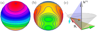
Figure 1: A tangential vector field on a sphere can be decomposed into (a) the curl-free component $\nabla_{s}\,\mathcal{E}$ and (b) the divergence-free component $\nabla_{s}\times\mathcal{G}$. (c) shows the gradient field $\mathbf{h}^{\rm eq}_{i}=-\partial\mathcal{E}/\partial\mathbf{S}_{i}$, which can be viewed as a quasi-equilibrium exchange field, and the curl-field $\mathbf{h}^{\rm neq}_{i}=-\mathbf{S}_{i}\times\partial\mathcal{G}/\partial\mathbf{S}_{i}$, which corresponds to the nonequilibrium force, and their respective torques $\mathbf{T}^{\rm eq}_{i}=\mathbf{h}^{\rm eq}_{i}\times\mathbf{S}_{i}$ and $\mathbf{T}^{\rm neq}_{i}=\mathbf{h}^{\rm neq}_{i}\times\mathbf{S}_{i}$.

Importantly, the generalized force formula in Eq. (3) now allows us to generalize the BP-type NN model for the nonequilibrium electron forces. To this end, we partition the two potentials into local contributions, namely $\mathcal{E}=\sum_{i}\epsilon_{i}$ and $\mathcal{G}=\sum_{i}\gamma_{i}$, based on the principle of locality kohn96 ; prodan05 . These two local energies $\epsilon_{i}$ and $\gamma_{i}$ are assumed to depend only on the local magnetic environment $\mathcal{C}_{i}$ through two universal functions $\varepsilon(\cdot)$ and $\chi(\cdot)$ for a given electronic model. Consequently, the dependence of the two potential energies on the spin configuration $\{\mathbf{S}_{i}\}$ can be expressed as

$$\mathcal{E}(\{\mathbf{S}_{j}\})=\sum_{i}\varepsilon(\mathcal{C}_{i}),\quad\quad\mathcal{G}(\{\mathbf{S}_{j}\})=\sum_{i}\chi(\mathcal{C}_{i}),\quad$$ (5)

In practice, the magnetic environment $\mathcal{C}_{i}$ can be defined as the spin configuration within some cutoff radius $R_{c}$ from the $i$-th spin, i.e. $\mathcal{C}_{i}=\bigl{\{}\mathbf{S}_{j}\,\big{|}\,|\mathbf{r}_{j}-\mathbf{r}_{i}|\leq R_{c}\bigr{\}}$. The complex dependences of local energies on $\mathcal{C}_{i}$ are approximated by a deep-learning NN as shown in Fig. 2. Finally, the forces Eq. (3) acting on spins are obtained from automatic differentiation of the two potentials.

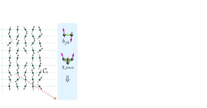
Figure 2: Schematic diagram of neural-network (NN) potential model based on the generalized force expression Eq.(3) for out-of-equilibrium itinerant spin system.

The above ML framework is general and can be used to represent spin forces in any nonequilibrium electron systems. In the following, we apply it to model the forces computed from the nonequilibrium Green’s functions (NEGF) method meir92 ; jauho94 ; datta95 ; haug08 ; diventra08 for the well-studied itinerant s-d spin model slonczewski96 ; berger96 ; brataas12 ; zhang04 ; yunoki98 under external voltage stress. We consider a square-lattice s-d system sandwiched by two electrodes in a capacitor structure. The total Hamiltonian is given by $\mathcal{H}_{\rm tot}=\mathcal{H}_{\rm sd}+\mathcal{H}_{\rm res}$, with

$$\mathcal{H}_{\rm sd}=-t_{\rm nn}\sum_{\langle ij\rangle}\bigl{(}c^{\dagger}_{i\alpha}c^{\;}_{j\alpha}+\mbox{h.c.}\bigr{)}-J\sum_{i}\mathbf{S}_{i}\cdot c^{\dagger}_{i\alpha}\bm{\sigma}^{\;}_{\alpha\beta}c^{\;}_{i\beta},\qquad$$ (6)

and $\mathcal{H}_{\rm res}$ describes the electrodes and the reservoir bath degrees of freedom, as well as their coupling to the sd-model in the center. The effects of the reservoir fermions can be subsumed into a self-energy $\bm{\Sigma}^{r}$ in the retarded Green’s function: $\mathbf{G}^{r}(\epsilon)=[\epsilon\mathbf{I}-\mathbf{H}_{\rm sd}-\bm{\Sigma}^{r}(\epsilon)]^{-1}$, where $\mathbf{H}_{\rm sd}$ is matrix representation of the sd Hamiltonian. Next, the lesser Green’s function can be obtained using the Keldysh formula for quasi-steady electron states: $\mathbf{G}^{<}(\epsilon)=\mathbf{G}^{r}(\epsilon)\bm{\Sigma}^{<}(\epsilon)\mathbf{G}^{a}(\epsilon)$, where the lesser self-energy $\bm{\Sigma}^{<}$ is related to the $\bm{\Sigma}^{r}$ through the dissipation-fluctuation theorem. The electronic force on the spins, which is obtained from the generalized Hellmann-Feynman theorem, can then be computed from the lesser Green’s function stamenova05 ; salahuddin06 ; xie17 ; petrovic18 ; dolui20 ; chern21

$$\mathbf{H}_{i}=-\biggl{\langle}\frac{\partial\hat{\mathcal{H}}_{\rm sd}}{\partial\mathbf{S}_{i}}\biggr{\rangle}=J\bm{\sigma}_{\beta\alpha}\int_{-\infty}^{+\infty}d\epsilon\,G^{<}_{i\alpha,i\beta}(\epsilon).$$ (7)

The exact forces computed from the NEGF method are used to train the NN model based on our generalized force formula. A magnetic descriptor developed in our previous work zhang21 is employed to translate the local magnetic environment $\mathcal{C}_{i}$ into a set of feature variables $\{G_{\ell}\}$ that are invariant under symmetry operations of the system. In particular, in order to ensure the global spin rotation symmetry of the s-d model, the bond variables $b_{jk}=\mathbf{S}_{j}\cdot\mathbf{S}_{k}$ of spin-pairs as well as the scalar chirality $\chi_{jkl}=\mathbf{S}_{j}\cdot\mathbf{S}_{k}\times\mathbf{S}_{l}$ of spin-triplets within the cutoff radius are used as the building blocks of the descriptor. These feature variables $\{G_{\ell}\}$ are fed into a fully connected NN, which in turn produces the two local energies $\epsilon_{i}$ and $\gamma_{i}$ associated with the $i$-th spin; see Fig. 2. Applying the NN model to compute all the local energies, the two potential energies $\mathcal{E}$ and $\mathcal{G}$ are then obtained through Eq. (5). Finally, the automatic differentiation of these two potentials gives the local forces $\mathbf{H}_{i}$ acting on the spins.

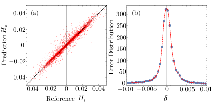
Figure 3: (a) The ML predicted forces versus the exact solution from the NEGF calculation for the s-d model with exchange coupling $J=3.8t_{\rm nn}$. (b) Normalized distribution of the prediction error of the perpendicular components of the forces.

A six-layer NN model is constructed and trained using PyTorch paszke19 from the NEGF-LLG simulations on a $30\times 24$ lattice. A total of 3200 snapshots, each of which provides a total of $\sim 600$ force data, are used for the training dataset. Contrary to the standard BP method where both forces and total energy are included in the training of the neural network, the loss function in our case is entirely given by the mean squared error of the perpendicular forces. Fig. 3 (a) shows the componentwise torques $\mathbf{S}_{i}\times\mathbf{H}_{i}$ predicted from our trained NN model versus the exact results. An excellent MSE of $8.97\times 10^{-6}$ is obtained from the trained NN model. The normalized distribution of the prediction error, shown in Fig. 3(b), is characterized by a rather small standard deviation of $\sigma=0.0014$.

We next incorporate the NN potential model into the LLG dynamics for the simulation of the voltage-driven domain-wall propagation in the square-lattice s-d model. The system is initially in an insulating antiferromagnetic (AFM) state with a spectral gap $\Delta E_{g}=2J$. An external voltage $V$ is applied to the two electrodes, which couple to the system at the left and right edges. When the chemical potential of one electrode is lowered to the eigen-energies of the in-gap edge modes, an instability towards the ferromagnetic (FM) ordering is triggered as electrons are drained from the edge of the system into the electrode. This instability leads to the nucleation of the FM domains at the edge of the sample. The subsequent expansion of the FM domains transforms the system into the low-resistant metallic state.

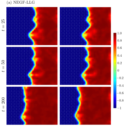
Figure 4: Domain wall propagation in a s-d system driven by an external voltage $eV=3.2t_{\rm nn}$. Comparison between (left) NEGF-LLG simulations and (right) ML-LLG simulations. The lattice size is $30\times 24$. The color bar indicates the local nearest-neighbor spin correlation $b_{ij}=\mathbf{S}_{i}\cdot\mathbf{S}_{j}$. Blue (red) area corresponds to AFM (FM) domains. The NEGF-LLG simulation was carried out at a low temperature of $T=0.01\,t_{\rm nn}$, while the ML simulation was performed without Langevin noise.

The spatio-temporal dynamics of this insulator-to-metal phase transformation has recently been systematically studied based on the NEGF-LLG simulations chern21 . The kinetics of the nonequilibrium phase transition described above is essentially governed by the propagation of the FM-AFM domain walls. Fig. 4 shows the propagation of domain walls obtained from the NEGF-LLG as well as the ML-LLG simulations on a $30\times 24$ square lattice. The same initial state with a well-developed FM-AFM domain wall was used for both simulations. The domain-wall position averaged over the transverse $y$-direction is plotted in Fig. 5(a) as a function of time for both the NEGF and ML-LLD simulations. Importantly, these comparisons demonstrate that our NN model not only is capable of predicting the nonequilibrium forces, but also can be used to accurately reproduce the nonequilibrium dynamical process of voltage-driven domain-wall propagation. The small discrepancy can be attributed to the random Langevin noise in the NEGF-LLG simulation and the force prediction error of the ML model.

A useful by-product of our NN model is the partition of the electron forces in Eq. (7), into the quasi-equilibrium $\mathbf{h}^{\rm eq}$ and nonequilibrium $\mathbf{h}^{\rm neq}$ components. As demonstrated in Fig. 1(c), the quasi-equilibrium torque $\mathbf{T}^{\rm eq}_{i}=\mathbf{h}^{\rm eq}\times\mathbf{S}_{i}$ is responsible for the precession motion of spins along contours of constant energy $\mathcal{E}$. On the other hand, the nonequilibrium torque $\mathbf{T}^{\rm neq}_{i}=\mathbf{h}_{i}^{\rm neq}\times\mathbf{S}_{i}$ often points to a direction away from the (quasi) equilibrium field, thus acting similar to the so-called anti-damping torques brataas12 ; ralph08 ; salahuddin08 . Fig. 5(b) shows a histogram of the ratio of these two torque components for spins in the vicinity of the AFM-FM domain walls. As expected, the driving force of the domain-wall propagation is dominated by the nonequilibrium forces.

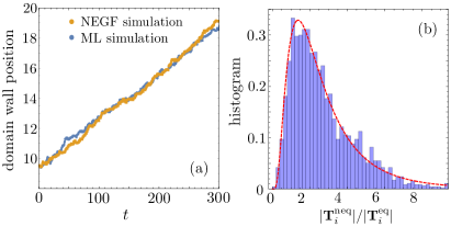
Figure 5: (a) Average position of FM-AFM domain, obtained from NEGF-LLG and ML-LLG simulations, as a function of time during the voltage-driven insulator to metal transition of the s-d model. (b) histogram of the ratio $|\mathbf{T}^{\rm neq}_{i}|/|\mathbf{T}^{\rm eq}_{i}|$ predicted by the NN model for the simulation of domain-wall propagation. Here $\mathbf{T}^{\rm eq}_{i}=\mathbf{S}_{i}\times\partial\mathcal{E}/\partial\mathbf{S}_{i}$ is the quasi-equilibrium torque, and $\mathbf{T}^{\rm neq}_{i}=\mathbf{S}_{i}\times(\mathbf{S}_{i}\times\partial\mathcal{G}/\partial\mathbf{S}_{i})$ is the non-equilibrium torque in the generalized LLG Eq. (4).

To summarize, we have developed a new potential theory of the nonequilibrium forces for the Landau-Lifshitz spin dynamics. This formulation allows us to generalize the Behler-Parrinello scheme, which is fundamental to most ML potentials for equilibrium quantum molecular dynamics and spin dynamics methods, to the modeling the electronic forces in out-of-equilibrium systems. We demonstrate our approach by developing a neural network model that successfully predicts the electronic forces computed from the nonequilibrium Green’s function method for a driven s-d model. Integrating the ML potential with the LLG simulations, we further show that the nonequilibrium process of voltage-driven domain-wall motion can be accurately reproduced by the trained neural network model.

Our work marks the first crucial step towards the multi-scale dynamical modeling of out-of-equilibrium quantum materials based on ML methods. In addition to the dynamical modeling of voltage-driven insulator-to-metal transition as demonstrated in this work, our ML formulation is also capable of describing the current-induced spin-transfer torques, which play a crucial role in the field of spintronics. The ML potential proposed in this work thus lays the groundwork for large-scale Landau-Lifshitz dynamics simulations with the desired quantum accuracy for the nonequilibrium electron forces, such as the spin-transfer torques. Finally, we note that our results cannot be directly applied to the atomic forces. Much work is required to develop a similar framework for the ML-potential for nonequilibrium quantum MD simulations.

- (1) G. Carleo, I. Cirac, K. Cranmer, L. Daudet, M. Schuld, N. Tishby, L. Vogt-Maranto, and L. Zdeborová, Machine learning and the physical sciences, Rev. Mod. Phys. 91, 045002 (2019).
- (2) S. D. Sarma, D.-L. Deng, and L.-M. Duan, Machine learning meets quantum physics, Phys. Today 72, 48 (2019).
- (3) E. Bedolla, L. C. Padierna, and R. Castaneda-Priego, Machine learning for condensed matter physics, J. Phys.: Condens. Matter 33, 053001 (2021).
- (4) J. Carrasquilla and R. G. Melko, Machine learning phases of matter, Nat. Phys. 13, 431 (2017).
- (5) E. P. Van Nieuwenburg, Y.-H. Liu, and S. D. Huber, Learning phase transitions by confusion, Nat. Phys. 13, 435 (2017).
- (6) Y. Zhang and E.-A. Kim, Quantum Loop Topography for Machine Learning, Phys. Rev. Lett. 118, 216401(2017).
- (7) F. Schindler, N. Regnault, and T. Neupert, Probing many-body localization with neural networks, Phys. Rev. B 95, 245134 (2017).
- (8) J. Venderley, V. Khemani, and E.-A. Kim, Machine Learning Out-of-Equilibrium Phases of Matter, Phys. Rev. Lett. 120, 257204 (2018).
- (9) G. Carleo and M. Troyer, Solving the quantum many-body problem with artificial neural networks, Science 355, 602 (2017).
- (10) Y. Nomura, A. S. Darmawan, Y. Yamaji, and M. Imada, Restricted Boltzmann machine learning for solving strongly correlated quantum systems, Phys. Rev. B 96, 205152 (2017).
- (11) M. Rupp, A. Tkatchenko, K.-R. Müller, and O. A. von Lilienfeld, Fast and Accurate Modeling of Molecular Atomization Energies with Machine Learning, Phys. Rev. Lett. 108, 058301 (2012).
- (12) J. C. Snyder, M. Rupp, K. Hansen, K.-R. Müller, and K. Burke, Finding Density Functionals with Machine Learning, Phys. Rev. Lett. 108, 253002 (2012).
- (13) F. Brockherde, L. Vogt, L. Li, M. E. Tuckerman, K. Burke, and K.-R. Müller, Bypassing the Kohn-Sham equations with machine learning, Nat. Commun. 8, 872 (2017).
- (14) K. T. Schütt, M. Gastegger, A. Tkatchenko, K.-R. Müller, and R. J. Maurer, Unifying machine learning and quantum chemistry with a deep neural network for molecular wavefunctions, Nat. Commun. 10, 5024 (2019).
- (15) S. Wang, K. Fan, N. Luo, Y. Cao, F. Wu, C. Zhang, K. A. Heller, and L. You, Massive computational acceleration by using neural networks to emulate mechanism-based biological models, Nat. Commun. 10, 4354 (2019).
- (16) M. Tsubaki and T. Mizoguchi, Quantum Deep Field: Data-Driven Wave Function, Electron Density Generation, and Atomization Energy Prediction and Extrapolation with Machine Learning, Phys. Rev. Lett. 125, 206401 (2020).
- (17) M. Bürkle, U. Perera, F. Gimbert, H. Nakamura, M. Kawata, and Y. Asai, Deep-Learning Approach to First-Principles Transport Simulations, Phys. Rev. Lett. 126, 177701 (2021).
- (18) L. Huang and L. Wang, Accelerated Monte Carlo simulations with restricted Boltzmann machines, Phys. Rev. B 95, 035105 (2017).
- (19) J. Liu, Y. Qi, Z. Y. Meng, and L. Fu, Self-learning Monte Carlo method, Phys. Rev. B 95, 041101(R) (2017).
- (20) J. Liu, H. Shen, Y. Qi, Z. Y. Meng, and L. Fu, Self-learning Monte Carlo method and cumulative update in fermion systems, Phys. Rev. B 95, 241104(R) (2017).
- (21) Y. Nagai, H. Shen, Y. Qi, J. Liu, and L. Fu, Self-learning Monte Carlo method: Continuous-time algorithm, Phys. Rev. B 96, 161102(R) (2017).
- (22) C. Chen, X. Y. Xu, J. Liu, G. Batrouni, R. Scalettar, and Z. Y. Meng, Symmetry-enforced self-learning Monte Carlo method applied to the Holstein model, Phys. Rev. B 98, 041102 (2018).
- (23) J. Behler and M. Parrinello, Generalized Neural-Network Representation of High-Dimensional Potential-Energy Surfaces, Phys. Rev. Lett. 98, 146401 (2007).
- (24) A. P. Bartók, M. C. Payne, R. Kondor, G. Csányi, Gaussian Approximation Potentials: The Accuracy of Quantum Mechanics, without the Electrons, Phys. Rev. Lett. 104, 136403 (2010).
- (25) Z. Li, J. R. Kermode, and A. De Vita, Molecular Dynamics with On-the-Fly Machine Learning of Quantum-Mechanical Forces, Phys. Rev. Lett. 114, 096405 (2015).
- (26) V. Botu, R. Batra, J. Chapman, and R. Ramprasad, Machine Learning Force Fields: Construction, Validation, and Outlook, J. Phys. Chem. C 121, 511 (2017).
- (27) Y. Li, H. Li, F. C. Pickard IV, B. Narayanan, F. G. Sen, M. K. Chan, S. K. Sankaranarayanan, B. R. Brooks, and B. Roux, Machine Learning Force Field Parameters from Ab Initio Data, J. Chem. Theory Comput. 13, 4492 (2017).
- (28) J. S. Smith, O. Isayev, and A. E. Roitberg, ANI-1: an extensible neural network potential with DFT accuracy at force field computational cost, Chem. Sci. 8, 3192 (2017).
- (29) L. Zhang, J. Han, H. Wang, R. Car, and Weinan E, Deep Potential Molecular Dynamics: A Scalable Model with the Accuracy of Quantum Mechanics, Phys. Rev. Lett. 120, 143001 (2018).
- (30) J. Behler, Perspective: Machine learning potentials for atomistic simulations, J. Chem. Phys. 145, 170901 (2016).
- (31) V. L. Deringer, M. A. Caro, and G. Csányi, Machine learning interatomic potentials as emerging tools for materials science, Adv. Mater. 31, 1902765 (2019).
- (32) R. T. McGibbon, A. G. Taube, A. G. Donchev, K. Siva, F. Hernández, C. Hargus, K.-H. Law, J. L. Klepeis, and D. E. Shaw, Improving the accuracy of Moller-Plesset perturbation theory with neural networks, J. Chem. Phys. 147, 161725 (2017).
- (33) H. Suwa, J. S. Smith, N. Lubbers, C.D. Batista, G.-W. Chern, and K. Barros, Machine learning for molecular dynamics with strongly correlated electrons, Phys. Rev. B 99, 161107 (2019).
- (34) T. Mueller, A. Hernandez, and C. Wang, Machine learning for interatomic potential models, J. Chem. Phys. 152, 050902 (2020).
- (35) D. Marx and J. Hutter, Ab initio molecular dynamics: basic theory and advanced methods (Cambridge University Press, Cambridge, 2009).
- (36) K. Walter, Density functional and density matrix method scaling linearly with the number of atoms, Phys. Rev. Lett. 76(17), 3168.
- (37) E. Prodan, and K. Walter, Nearsightedness of electronic matter, Proc. Natl. Acad. Sci. U.S.A. 102.33 (2005): 11635-11638.
- (38) Y. Nagai, M. Okumura, and A. Tanaka, Self-learning Monte Carlo method with Behler-Parrinello neural networks, Phys. Rev. B 101, 115111 (2020).
- (39) J. Ma, P. Zhang, Y. Tan, A. W. Ghosh, and G.-W. Chern, Machine learning electron correlation in a disordered medium, Phys. Rev. B 99, 085118 (2019).
- (40) S. Zhang, P. Zhang, and G.-W. Chern, Anomalous phase separation and hidden coarsening of super-clusters in the Falicov-Kimball model, arXiv:2105.13304 (2021).
- (41) P. Zhang, P. Saha, and G.-W. Chern, Machine learning dynamics of phase separation in correlated electron magnets, arXiv:2006.04205 (2020).
- (42) P. Zhang and G.-W. Chern, Arrested Phase Separation in Double-Exchange Models: Large-Scale Simulation Enabled by Machine Learning, Phys. Rev. Lett. 127, 146401 (2021).
- (43) J.-T.Lü, M. Brandbyge, P. Hedegard, T. N. Todorov, and D. Dundas, Current-induced atomic dynamics, instabilities, and Raman signals: Quasiclassical Langevin equation approach, Phys. Rev. B 85, 245444 (2012).
- (44) T. N. Todorov, D. Dundas, and E. J. McEniry, Nonconservative generalized current-induced forces, Phys. Rev. B 81, 075416 (2010).
- (45) D. Dundas, E. J. McEniry, and T. N. Todorov, Current-driven atomic waterwheels, Nat. Nanotech. 4, 99 (2009).
- (46) M. Di Ventra and S. T. Pantelides, Hellmann-Feynman theorem and the definition of forces in quantum time-dependent and transport problems, Phys. Rev. B 61, 16207 (2000).
- (47) J. C. Slonczewski, Current-driven excitation of magnetic multilayers, J. Magn. Magn. Mater. 159, L1 (1996).
- (48) L. Berger, Emission of spin waves by a magnetic multilayer traversed by a current, Phys. Rev. B 54, 9353 (1996).
- (49) A. Brataas, A. D. Kent, and H. Ohno, Current-induced torques in magnetic materials, Nat. Mater. 11, 372 (2012).
- (50) D. C. Ralph and M. D. Stiles, Spin transfer torques, J. Magn. Magn. Mater. 320, 1190, (2008).
- (51) S. Salahuddin, D. Datta, and S. Datta, Spin Transfer Torque as a Non-Conservative Pseudo-Field, arXiv:0811.3472 (2008).
- (52) S. Chmiela, A. Tkatchenko, H. E. Sauceda, I. Poltavsky, K.T.Schütt, and K.-R.Müller, Machine learning of accurate energy-conserving molecular force fields, Sci. Adv. 3, e1603015 (2017).
- (53) S. Chmiela, H. E. Sauceda, K.-R.Müller, and A. Tkatchenko, Towards exact molecular dynamics simulations with machine-learned force fields, Nat. Commun. 9, 3887 (2018).
- (54) J. F. Adams, Vector fields on spheres, Ann. Math. 75, 603 (1962).
- (55) P. N. Swarztrauber, The approximation of vector functions and their derivatives on the sphere, SIAM J. Numer. Anal. 18, 191 (1981).
- (56) M. Fan, D. Paul, T. C. M. Lee, and T. Matsuo, Modeling tangential vector fields on a sphere, J. Am. Stat. Assoc. 113, 1625 (2018).
- (57) Y. Meir and N. S. Wingreen, Landauer formula for the current through an interacting electron region, Phys. Rev. Lett. 68, 2512 (1992).
- (58) A.-P. Jauho, N. S. Wingreen, Y. Meir, Time-dependent transport in interacting and noninteracting resonant-tunneling systems, Phys. Rev. B 50, 5528 (1994).
- (59) S. Datta, Electronic Transport in Mesoscopic Systems (Cambridge University Press, Cambridge, 1995).
- (60) H. Haug and A.-P. Jauho, Quantum Kinetics in Transport and Optics of Semiconductors, Springer Series in Solid-State Sciences 123 (Springer-Verlag, Berlin, 2008).
- (61) M. Di Ventra, Electrical Transport in Nanoscale Systems (Cambridge University Press, Cambridge, 2008).
- (62) S. Zhang and Z. Li, Roles of Nonequilibrium Conduction Electrons on the Magnetization Dynamics of Ferromagnets, Phys. Rev. Lett. 93, 127204 (2004).
- (63) S. Yunoki, J. Hu, A. L. Malvezzi, A. Moreo, N. Furukawa, and E. Dagotto, Phase Seperation in Electronic Models for Manganites, Phys. Rev. Lett. 80, 845 (1998).
- (64) M. Stamenova, S. Sanvito, and T. N. Todorov, Current-driven magnetic rearrangements in spin-polarized point contacts, Phys. Rev. B 72, 134407 (2005).
- (65) S. Salahuddin and S. Datta, Self-consistent simulation of quantum transport and magnetization dynamics in spin-torque based devices, Appl. Phys. Lett. 89, 153504 (2006).
- (66) Y. Xie, J. Ma, S. Ganguly, and A. W. Ghosh, From materials to systems: a multiscale analysis of nanomagnetic switching, J. Comput. Electron. 16, 1201 (2017).
- (67) M. D. Petrović, B. S. Popescu, U. Bajpai, P. Plechac, and B. K. Nikolić, Spin and Charge Pumping by a Steady or Pulse-Current-Driven Magnetic Domain Wall: A Self-Consistent Multiscale Time-Dependent Quantum-Classical Hybrid Approach, Phys. Rev. Appl. 10, 054038 (2018).
- (68) K. Dolui, M. D. Petrović, K. Zollner, P. Plechác, J. Fabian, and B. K. Nikolić, Proximity Spin-Orbit Torque on a Two-Dimensional Magnet within van der Walls Heterostructure: Current-Driven Antiferromagnet-to-Ferromagnet Reversible Nonequilibrium Phase Transition in BIlayer CrI3, Nano Lett. 20, 2288 (2020).
- (69) G.-W. Chern, Spatio-temporal dynamics of voltage-induced resistance transition in the double-exchange model, arXiv:2105.11076 (2021).
- (70) A. Paszke, S. Gross, F. Massa, A. Lerer, J. Bradbury, G. Chanan, T. Killeen, Z. Lin, N. Gimelshein, L. Antiga, and A. Desmaison, PyTorch: An imperative style, high-performance deep learning library. In Advances in Neural Information Processing Systems 2019 (pp. 8024-8035).