Domain Adaptation for Simulation-Based Dark Matter Searches
Using Strong Gravitational Lensing

Abstract

Clues to the identity of dark matter have remained surprisingly elusive, given the scope of experimental programs aimed at its identification. While terrestrial experiments may be able to nail down a model, an alternative, and equally promising, method is to identify dark matter based on astrophysical or cosmological signatures. A particularly sensitive approach is based on the unique signature of dark matter substructure on galaxy-galaxy strong lensing images. Machine learning applications have been explored in detail for extracting just this signal. With limited availability of high quality strong lensing data, these approaches have exclusively relied on simulations. Naturally, due to the differences with the real instrumental data, machine learning models trained on simulations are expected to lose accuracy when applied to real data. This is where domain adaptation can serve as a crucial bridge between simulations and real data applications. In this work, we demonstrate the power of domain adaptation techniques applied to strong gravitational lensing data with dark matter substructure. We show with simulated data sets of varying complexity, that domain adaptation can significantly mitigate the losses in the model performance. This technique can help domain experts build and apply better machine learning models for extracting useful information from strong gravitational lensing data expected from the upcoming surveys.

I Introduction

One of the great achievements of astrophysics in the last century was the realization by Zwicky, Rubin and others that the observed baryonic mass (stars, galaxies, etc.) was not consistent with the dynamics of galaxies and clusters. A natural solution to this problem was to consider some unseen matter that compensated for this discrepancy, or so-called dark matter. Presently, all efforts aimed at extracting a non-gravitational signature of dark matter have come up empty Drukier et al. (1986); Goodman and Witten (1985); Akerib et al. (2017); Cui et al. (2017); Aprile et al. (2018); Froborg and Duffy (2020); Fermi LAT Collaboration (2015); Geringer-Sameth et al. (2015); Albert et al. (2018); VERITAS Collaboration (2017); Rico (2020); MAGIC Collaboration (2016); IceCube Collaboration (2017); The Super-Kamiokande Collaboration (2015); Du et al. (2018); Graham et al. (2015); Kannike et al. (2020); Buch et al. (2020); Aaboud et al. (2019); Sirunyan, A. M. and Tumasyan, A. and Adam, W. and Asilar, E. and Bergauer, T., and et al. (2017). While this does not mean that dark matter can not communicate with Standard Model (SM) particles, as it may be the case that its SM couplings are strongly suppressed, there is also the possibility that such interactions do not exist.

Since its discovery, subsequent evidence for particle dark matter from its coupling to gravity is almost irrefutable Planck Collaboration (2016); L. Anderson, E. Aubourg et al. (2014); C. Heymans, L. van Waerbeke et al. (2012). However, the list of possible models that fit current constraints is still quite broad. A particularly well suited signature that can be used to distinguish among dark matter models is the morphology and distribution of its substructure within dark matter halos. Some promising directions for inferring the properties of substructure include tidal streams Ngan and Carlberg (2014); Carlberg (2016); Bovy (2016); Erkal et al. (2016); Shih et al. (2021); Benito et al. (2020) and astrometric observations Mishra-Sharma et al. (2020); Van Tilburg et al. (2018); Feldmann and Spolyar (2015); Sanderson et al. (2016); Vattis et al. (2020); Mishra-Sharma (2021); Pardo and Doré (2021). A particularly sensitive probe will be strong gravitational lensing Buckley and Peter (2018); Drlica-Wagner et al. (2019); Simon et al. (2019) for which we restrict ourselves in this article.

Strong lensing has already seen some promising success in extracting information about dark matter substructure, from lensed quasars S. Mao and P. Schneider (1998); J.W. Hsueh et al. (2017); N. Dalal and C.S. Kochanek (2002), observations with ALMA Y.D. Hezaveh et al. (2016), and extended lensing images S. Vegetti and L.V.E. Koopmans (2009a); L.V.E. Koopmans (2005); S. Vegetti and L.V.E. Koopmans (2009b). Various works have considered the expected signatures and methods to extract information about the underlying distribution of dark matter Daylan et al. (2018); Vegetti et al. (2010a); Daylan et al. (2018); Vegetti et al. (2010b).

More recently, there has been a plethora of applications of machine learning to this challenge, ranging from classification Alexander et al. (2020a); Diaz Rivero and Dvorkin (2020); Varma et al. (2020), regression Brehmer et al. (2019), segmentation analysis Ostdiek et al. (2020a, b), and anomaly detection Alexander et al. (2020b). To date, all works have exclusively focused on the application of these techniques to simulations, in large part due to the limited availability of strong lensing data; something that is anticipated to change in the near future with the commissioning of the Vera C. Rubin Observatory and the launch of Euclid Verma et al. (2019); Oguri and Marshall (2010). However, not unexpectedly, naively applying a model trained on simulations to real data is not likely to be very successful, as the data idiosyncrasies relative to simulations will significantly diminish the accuracy of the model. A promising method to bridge the gap between a model trained on simulations and real world data is based on the technique of domain adaptation (DA) Ben-David et al. (2010).

A subset of transfer learning, domain adaptation is focused on the generalization of the model across different domains or data sets drawn from different underlying distributions. Concretely, the goal of domain adaptation is to adapt a model trained on one data set (source) by generalizing it to another domain (target), where the objective of the model is unchanged. In practice domain adaptation can be realized in several ways, including supervised, semi-supervised, and unsupervised fashions Motiian et al. (2017); Donahue et al. (2013); Farahani et al. (2020).

Domain adaptation techniques have been used in a wide variety of applications related to computer vision, such as adapting a model trained on synthetic images to real images Peng et al. (2017), simple to complex images Tzeng et al. (2017) and virtual worlds with controlled data to the real world Schmidt et al. (2021).

Recently, Ćiprijanović et al. (2021) used unsupervised domain adaptation (UDA) to classify merging galaxies. Doing so achieved promising results, with an increase of up to $19\%$ in accuracy when compared to a model trained only on simulations. This work also showed that models trained without domain adaptation, achieved a poor accuracy on real data. In another work Ostdiek et al. (2020b) used domain adaptation to generalize an image segmentation algorithm to different gravitational lensing systems for subhalo detection.

In this work, we consider several domain adaptation algorithms to establish a proof-of-concept application for dark matter searches in strong gravitational lensing. Given the present lack of sufficient real data, we use two datasets with differing levels of complexity of strong lensing simulations to carefully test the performance of domain adaptation prior to eventual applications to real data. We evaluate the application of models trained on the source data set to identify various types of dark matter substructure on the target data set. We compare the performance of several domain adaptation algorithms, to find the best model. We additionally investigate equivariant neural network models that incorporate a known group symmetry, to further enhance the performance of domain adaptation.

We begin with a brief review of dark matter substructure and also discuss several lensing signatures in Section II. We then focus on the details of strong lensing simulations in Section III, followed by a summary of domain adaptation algorithms in Section IV. We present our main results in Section V, followed by the discussion and outlook in Section VI.

II Dark Matter Detection and Strong Gravitational Lensing

II.1 Dark Matter Substructure

The $\Lambda$ Cold Dark Matter ($\Lambda$CDM) model envisions near scale invariant density fluctuations, present in the early universe, serving as seeds of large-scale structure via hierarchical structure formation. Concretely, structures such as dark matter halos are formed from the coalescence of smaller halos Kauffmann et al. (1993). Evidence for such merges has been observed in our Galaxy Chiti et al. (2021); Necib et al. (2020a, b) and is a general prediction of N-body simulations where evidence of mergers should remain largely in tact. The distribution of subhalos masses is expected to follow a power law distribution,

$$\frac{dN}{dm}\propto m^{\beta},$$ (1)

where $\beta\sim-1.9$ has been found from simulations Springel et al. (2008); Madau et al. (2008).

Comparison between simulation and observation indicates good agreement with $\Lambda$CDM on large-scales Planck Collaboration (2016); L. Anderson, E. Aubourg et al. (2014); C. Heymans, L. van Waerbeke et al. (2012). However, discrepancies begin to arise on smaller, sub-galactic scales. These include the core-vs-cusp Burkert (1995); Oh et al. (2015), too big to fail Boylan-Kolchin et al. (2011), missing satellite Moore et al. (1999); Klypin et al. (1999); Bullock and Boylan-Kolchin (2017), and diversity problems Oh et al. (2015). While it may be the case that these problems can be addressed with a better understanding of the astrophysics, e.g. baryonic feedback Benítez-Llambay et al. (2019), it is imperative that we consider the manifestations of other theories beyond $\Lambda$CDM.

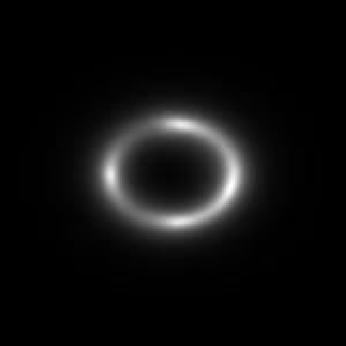
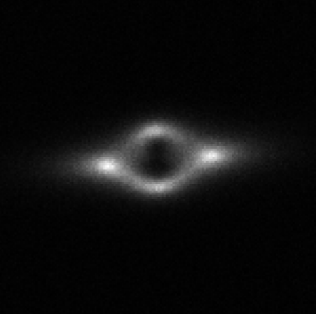
Figure 1: Example images from the source (left) and target (right) data set.

Two natural directions to consider are a modification to the general theory of relativity, such as BF coupled Alexander and Carballo-Rubio (2020); Alexander et al. (2020c, 2021a) or Chern-Simons gravity Jackiw and Pi (2003); Alexander and Yunes (2009), or alternatives to cold non-interactive dark matter. In the context of this paper, we will focus on the latter. An example of a dark matter model that addresses several of the tensions mentioned above is condensate dark matter, which can be realized in the context of Bose-Einstein (BEC) Sin (1994); Silverman and Mallett (2002); Hu et al. (2000); Sikivie and Yang (2009); Hui et al. (2017); Berezhiani and Khoury (2015); Ferreira et al. (2019) or Bardeen-Cooper-Schreifer(BCS) Alexander and Cormack (2017); Alexander et al. (2018, 2021b) condensates. A concrete and well motivated model is the axion. As the Goldstone boson of a broken U(1) symmetry, axions were originally introduced as a solution to the Strong-CP problem Peccei and Quinn (1977); Wilczek (1978); Weinberg (1978). Shortly thereafter, it was recognized that they were a promising dark matter candidate Preskill et al. (1983); Abbott and Sikivie (1983); Dine and Fischler (1983). Very light axions are particularly well suited to address some of the issues with structure on sub-galactic scales. Axions with masses $\sim 1\times 10^{-23}$ eV have a de Broglie wavelength on kpc scales, which realizes a natural solution to the core-vs-cusp problem. Additionally, light axions can form subhalos but can also form substructures quite different from standard CDM. These include vortices, disks, and interference patterns T. Rindler-Daller, P. R. Shapiro (2012); Hui (2021); Hui et al. (2021); Alexander et al. (2019, 2021c).

While we will not consider their impact in this work, it is important to also consider line of sight halos, i.e. interlopers Çağan Şengül et al. (2020); McCully et al. (2017); Despali et al. (2018); Gilman et al. (2019). In some cases their influence may dominate the signal of substructure, so it is important to take care that they are not incorrectly associated with the dark matter halo when working with real data sets (see for example Şengül et al. (2021)).

II.2 Strong Lensing Theory

A powerful probe of dark matter substructure is strong gravitational lensing; an effect which is most pronounced near extended lensing arcs. Any over or under densities along the line of sight for an observer yields the lens equation, realized as an integral over an induced gravitational potential Narayan and Bartelmann (1997),

$$\vec{\beta}=\vec{\theta}-\frac{2}{c^{2}}\frac{D_{LS}}{D_{S}D_{L}}\vec{\nabla}\int dz~{}\Psi(\vec{r}),$$ (2)

where $D_{LS},D_{L},D_{S}$ are the angular diameter distances from the lens to the source, the lens to the observer, and the source to observer. The last term on the r.h.s. of Equation 2 is known as the deflection angle, $\vec{\alpha}$, and is related via a perpendicular derivative to the the lensing potential, $\Psi_{;\perp}=\alpha$. The lensing potential can be shown to be related to matter density via a Poisson equation for gravitational lensing,

$$\nabla^{2}\Psi=2\kappa,$$ (3)

implying that lensing from separate sources, a DM halo and its subhalos, is a sum of deflection angles,

$$\vec{\alpha}=\sum_{\rm all~{}matter}\vec{\alpha}_{i},$$ (4)

where $\vec{\alpha}_{i}$ could represent a DM halo, subhalos, vortices, external shear, interlopers etc.

III Strong Lensing Simulations

Similar to Alexander et al. (2020a, b) we consider data sets of three substructure classes; no substructure, subhalos of CDM, and vortex substructure of superfluid type dark matter. The parameters for the simulations are complied in Table 1. The strong lensing images are simulated with PyAutolens Nightingale and Dye (2015); Nightingale et al. (2018). The data are sized $150\times 150$ pixels with a scale $0.5^{\prime\prime}/$pixel. The light from lensed background galaxies is modeled as a simple Sersic profile and the signal-to-noise ratio (SNR) of the lensing arcs are consistent with real lensing data – $SNR\sim 20$ Bolton et al. (2008) – by appropriate inclusion of backgrounds and noise. We further consider the modifications induced by a point-spread function (PSF), modeled as an Airy disk with first zero-crossing $\sigma_{\rm psf}\lesssim 1^{\prime\prime}$.

We ensure that the total fraction of mass in substructure, $f_{sub}$, is of $\mathcal{O}(1\%)$. We constrain the simulations such that the total mass of the halo, including substructure, is always equal to $1\times 10^{12}~{}{\rm M}_{\odot}$. This is done to ensure that classification algorithms don’t simply recognize simulations without substructure as less massive on average. When simulating substructure for CDM we draw subhalo masses from from Equation 1 for a total number of sources taken from a Poisson draw with $\mu=25$, consistent with the expected number of subhalos for our field of view and redshift range Díaz Rivero et al. (2018). We model vortices of superfluid dark matter as uniform density strings of mass of varying length and orientation – a valid approximation at cosmological distances. Beyond the effects of substructure, we also include the impact of external shear due to large-scale structure.

The inclusion of the effects of substructure in our simulations can be understood from the linearity of the Poisson equation, Equation 3, which implies the total lensing is just the sum of the individual contributions,

$$\alpha=\alpha_{LSS}+\alpha_{halo}+\alpha_{halo-sub},$$ (5)

where $\alpha_{LSS}$ is the external shear from large-scale-structure, $~{}\alpha_{halo}$ the lensing from the halo and $~{}\alpha_{halo-sub}$ for halo substructure. It then follows that the location of an image can be found from a modified form of the lens equation, Equation 2,

$$\beta^{i}=\theta^{i}-\alpha^{i}_{LSS}-\alpha^{i}_{halo}-\alpha^{i}_{halo-sub}.$$ (6)

Domain adaptation requires at least two data sets, the source and the target. In this work we consider two distinct simulations as source and target data sets. The biggest difference between source and target data sets is that source images are held at fixed redshift, while the target data set allows the redshifts to float over a range of values for both the lensed and lensing galaxy. Additionally, the SNR in the target data set varies over a larger range of values, $10\lesssim{\rm SNR}\lesssim 30$, consistent with the challenges associated with variable source distances. Thus, the target data set constitutes a more challenging sample for identifying dark matter substructure - this difference is easy to see by eye in Figure 1 for example lenses from both classes. Thus, it will be our goal to successfully adapt and evaluate the algorithms trained on the source data set to the target data set.

Table 1: Parameters with distributions and priors used in the simulation of strong lensing images. Parameters with subscript $s$ & $t$ correspond to parameters for source and target data sets respectively. Note that only a single type of substructure was used per image.

DM Halo
Param.	Dist.	Priors	Details
$\theta_{x}$	fixed	0	x position
$\theta_{y}$	fixed	0	y position
zs	fixed	0.5	redshift
zt	uniform	[0.4,0.6]	redshift
$M_{\rm TOT}$	fixed	1e12	total halo mass in ${\rm M}_{\odot}$
Ext. Shear
Param.	Dist.	Priors	Details
$\gamma_{ext}$	uniform	[0.0, 0.3]	magnitude
$\phi_{ext}$	uniform	[0, 2$\pi$]	angle
Lensed Gal.
Param.	Dist.	Priors	Details
$r$	uniform	[0, 0.5]	radial distance from center
$\phi_{bk}$	uniform	[0, 2$\pi$]	orientation from y axis
zs	fixed	1.0	redshift
zt	uniform	[0.8,1.2]	redshift
e	uniform	[0.4, 1.0]	axis ratio
$\phi$	uniform	[0, 2$\pi$]	orientation to y axis
n	fixed	1.5	Sersic index
R	uniform	[0.25,1]	effective radius
Vortex
Param.	Dist.	Priors	Details
$\theta_{x}$	normal	$[0.0,0.5]$	x position
$\theta_{y}$	normal	$[0.0,0.5]$	y position
$l$	uniform	[0.5,2.0]	length of vortex
$\phi_{vort}$	uniform	[0, 2$\pi$]	orientation from y axis
$m_{vort}$	uniform	[3.0,5.5]	% of mass in vortex
Subhalo
Param.	Dist.	Priors	Details
$r$	uniform	[0, 2.0]	radial distance from center
$N$	Poisson	$\mu$=25	number of subhalos
$\phi_{sh}$	uniform	[0, 2$\pi$]	orientation from y axis
$m_{sh}$	power law	[1e6,1e10]	subhalo mass in ${\rm M}_{\odot}$
$\beta_{sh}$	fixed	-1.9	power law index

IV Domain Adaptation

Our goal is to train a supervised model on a source data set and adapt it to a target data set. For this task we use ResNet-18 He et al. (2015), a Convolutional Neural Network (CNN), as our base architecture. This is the same architecture that has achieved top performance in previous applications to lensing data sets Alexander et al. (2020a, b); Vattis et al. (2020). More generally, CNNs are known to outperform other methods of classification for strong gravitational lenses Metcalf et al. (2019), nonetheless, as noted by Ćiprijanović et al. (2021), a model trained on simulations can perform poorly on real data.

To improve the performance of models trained on simulated data, we use unsupervised domain adaptation, which attempts to mitigate the effects of the domain shift between the source and the target domains. It enables a transfer of knowledge gained from a labeled source data set to a distinct unlabeled target data set, within the constraint that the objective remains the same French et al. (2018). Example source and target data are shown in Fig. 1. For our analysis we consider three UDA algorithms described below.

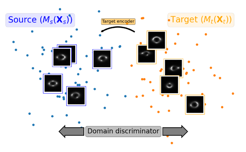
Figure 2: Depiction of target and source representations in the latent space of the encoder in ADDA. Images in blue are from the source domain and images in orange are from the target domain.

Table 2: Hyperparameters and augmentations used to train the UDA algorithms.

Method	Hyperparameters	Hyperparameter values	Augmentations
	Learning rate	$1\times 10^{-3}$	Horizontal flips
Supervised	Weight decay	$5\times 10^{-5}$	Vertical flips
	Cyclic scheduler	True
	Learning rate target encoder	$1\times 10^{-5}$	Horizontal flips
ADDA	Learning rate target encoder	$1\times 10^{-4}$	Vertical flips
	Weight decay	$5\times 10^{-5}$
	Cyclic scheduler	False
	Learning rate	$1\times 10^{-3}$	Horizontal flips
AdaMatch	Tau	$0.9$	Vertical flips
	Weight decay	$5\times 10^{-5}$	Random autocontrast
	Cyclic scheduler	False	Gaussian blur
			Random invert
			Random adjust sharpness
			Random solarize
			Random affine transformations
	Learning rate	$1\times 10^{-3}$	Horizontal flips
Self-Ensemble	Weight of unsupervised loss	$3.0$	Vertical flips
	Weight decay	$5\times 10^{-5}$	Gaussian blur
	Cyclic scheduler	False

IV.1 Unsupervised Domain Adaptation Techniques

We first consider Adversarial Discriminative Domain Adaptation (ADDA) Tzeng et al. (2017), an adversarial adaptation method with the goal of minimizing the domain discrepancy distance through an adversarial objective with respect to a discriminator. Ideally the discriminator will be unable to distinguish between the source and the target distributions. We consider that we have access to source images $\mathbf{X}_{s}$ and labels $\mathbf{Y}_{s}$ that come from a source distribution $p_{s}(x,y)$ and also target images $\mathbf{X}_{t}$ from a target distribution $p_{t}(x,y)$. Our objective is to learn a target encoder $M_{t}$ and classifier $C_{t}$ that classifies $\mathbf{X}_{t}$ into $K$ classes.

Due to the fact that it is not possible to perform supervised learning on the target distribution, we learn a source encoder $M_{s}$ and a source classifier $C_{s}$. The encoder learns to map the input samples to a latent vector whose dimensionality is lower than the dimensionality of the input samples. With these networks trained, the distance between $M_{s}(\mathbf{X}_{s})$ and $M_{t}(\mathbf{X}_{t})$ is minimized, as illustrated in Fig. 2. Since we’re only minimizing the encoders, we can assume that $C_{s}=C_{t}=C$.

We train $M_{s}$ and $C$ using a standard supervised loss. Then, we train a discriminator $D$ that classifies if the encoded vector represents an image from the source domain or from the target domain using a standard supervised loss, where the labels indicate the origin domain. Finally, we train the $M_{t}$ using $D$. To evaluate a target image $\mathbf{X}_{t}$ we perform $C(M_{t}(\mathbf{X}_{t}))$.

We additionally evaluate two DA algorithms derived from semi-supervised learning. The first makes use of self-ensembling (Self-Ensemble) French et al. (2018) and is based on the mean teacher semi-supervised model Tarvainen and Valpola (2017). There are two networks in this method: a student network that is trained using gradient descent and a teacher network whose weights are an exponential moving average of the student’s. During training, the labeled source inputs are passed through the student network and the cross-entropy loss is taken. However, the unlabeled target inputs pass through both the student and teacher networks and the self-ensembling loss is used. It is computed as the mean-squared difference between the predictions created by the student and the teacher networks with different augmentations, dropout and noise parameters, and penalizes the difference in class prediction between the student and the teacher. This method also makes use of confidence thresholding and a class balancing loss term. The second semi-supervised method, AdaMatch Berthelot et al. (2021), uses weak and strong augmentations on both the source and target input images. During training the method also uses random logit interpolation, distribution alignment and relative confidence thresholding to achieve a better performance.

In additional to the baseline CNN models, we also consider an Equivariant Neural Network (ENN) Weiler and Cesa (2021) for substructure classification. ENNs can be thought of a generalization of a CNN that encode the representation of a useful symmetry, both global or local, such that its group convolutions are invariant symmetries present in the data. This is useful if there is a known symmetry in the problem. As we expect lensing images to have symmetries beyond simple translation, for example rotations, the flexibility of choosing different group representations is expected to improve the performance.

The ENN we use consists of a group equivariant convolutional neural network Cohen and Welling (2016) with six equivariant convolution blocks. We utilize the dihedral group $D_{2}$, whose symmetry mappings include the identity, rotations by $\pm\pi$ and horizontal/vertical reflections. The $D_{2}$ group structure can be visualized in Fig. 3. Each block is composed of a convolutional layer, a batch normalization layer and a ReLU activation function. After each pair of layers we perform channel-wise average-pooling and in the end we use a fully connected layer for multiclass classification. A schematic of the ENN architecture is presented in Fig. 4.

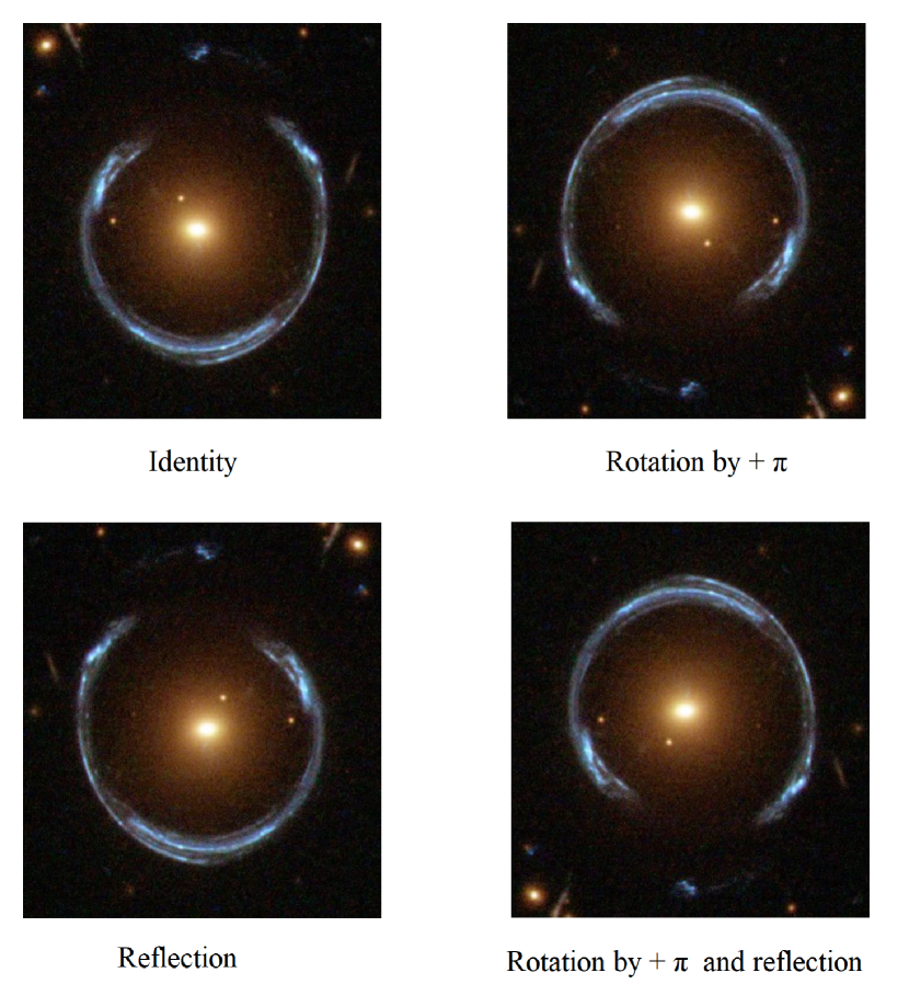
Figure 3: Visualization of the $D_{2}$ group structure for a real gravitational lens. Lensing image credit: ESA/Hubble & NASA.

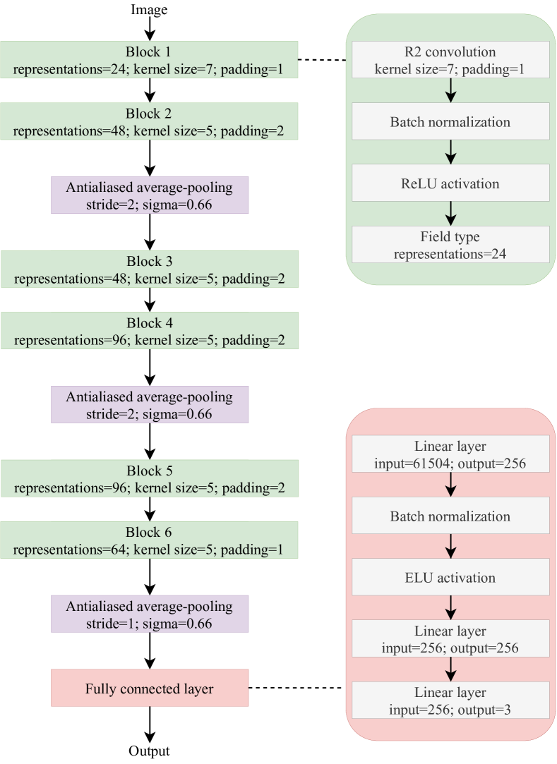
Figure 4: Schematic of the equivariant (ENN) architecture.

IV.2 Network Training

For training we use $30,000$ images for the source domain and $30,000$ images for the target domain; in both cases there are $10,000$ images per class. For validation we use $7,500$ images for the source domain and $7,500$ images for the target; in both cases there are $2,500$ images per class. We used the Adam optimizer Kingma and Ba (2017) to minimize our losses. We trained both ResNet-18 and the ENN for $200$ epochs, training with a patience of $15$ epochs, such that if the accuracy of the model does not improve in $15$ epochs we stop training. For final results, we considered the epoch that achieved the largest accuracy. Learning rate, weight decay and other hyperparameters were optimized through a hyperparameters search, and are available in Table 2.

We used random horizontal and random flips augmentations for both the source and target dataset. We also found that the best results were obtained after random zooming (in a range of $[0.8,1.2]$) and random rotations (in a range of $[0,90]$ degrees) on the source dataset. Two of the UDA algorithms, Self-Ensemble and AdaMatch, are also highly dependent on augmentations, and different augmentations were tested to find the optimal configurations. We utilize the area under the ROC curve (AUC) on the target validation set as the metric for classifier performance for all the models. All quoted AUC values are macro-averaged unless stated otherwise. All machine learning models were implemented using PyTorch Paszke et al. (2019a) and are run on a single NVIDIA Tesla P100 GPU.

V Results

We compare three different UDA techniques in the context of multi-class classification of three types of substructure: no substructure, CDM subhalos, and superfluid DM vortices. We employ two different base classifiers for each technique - ResNet-18 and an ENN. The parameters for our source and target data sets are shown in Table 1. Better results on all methods were achieved when starting UDA training with models that were pre-trained in a supervised fashion using source data, as discussed in Ćiprijanović et al. (2021). As such, our models were trained starting from models pre-trained on the source simulation data. Results from our analysis are shown in Tables 3 and 4 for ResNet-18 and the ENN respectively. ROC curves for both architectures are presented in Figure 5.

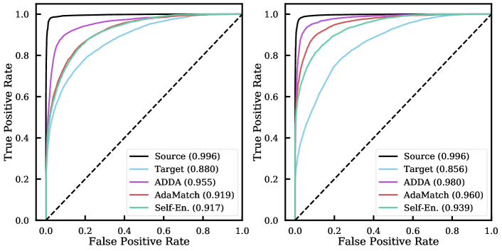
Figure 5: ROC-AUC curves for ResNet-18 (left) and ENN (right) based algorithms applied to our data set.

V.1 Domain Adaptation

We first train ResNet-18 on the source data set where it achieved a macro-averaged AUC $\approx~{}0.996$ and an accuracy of $\approx$ 97%. Applying this model to the target data set naively, i.e. without domain adaptation, results in an AUC of $\approx$ $0.880$ and accuracy of $\approx$ 59%, a significantly degraded performance, as anticipated.

Following the application of UDA techniques, we observe a significant improvement when applied to the target data set. AdaMatch and Self-Ensemble achieve an AUC of $\approx$ $0.919$ and $0.917$, respectively, which shows good improvement over the results obtained without domain adaptation. The top performing ResNet-18 based UDA model is ADDA. With a $\approx$ 9% improvement in AUC, at $\approx$ $0.955$, and accuracy of $\approx$ 86%, ADDA significantly improves the performance of our model on the target data set.

Considering the performance for individual classes, we find that ADDA achieves consistent AUC scores of $\approx 0.95$ for all three classes. This is in contrast to the performance on naive application, where no substructure and subhalos classification each had an AUC of $\approx 0.90$ and classification of vortices was severely degraded to an AUC of $\approx 0.80$. The baseline model applied to the source data set, on the other hand, had consistent performance on a class by class basis at $\approx 0.99$ AUC.

Table 3: Accuracy and macro-averaged area under the ROC curve (AUC) for the ResNet-18 classifier.

Method		Accuracy (%)		AUC
ADDA		$85.84$		$0.955$
AdaMatch		$75.55$		$0.919$
Self-Ensemble		$76.71$		$0.917$
Supervised (target)		$59.19$		$0.880$
Supervised (source)		$96.84$		$0.996$

V.2 Equivariant Domain Adaptation

With an AUC of $\approx$ 0.996 and accuracy of $\approx 91\%$, the ENN performance is commensurate with ResNet-18 on the source data set. The naive application to the test data set (i.e. no domain adaption) again results in degraded performance, realized with an AUC $\approx$ 0.856 and accuracy of $\approx$ 68%.

The Self-Ensemble and AdaMatch equivariant models again show improved performance relative to the naive case and with AUC scores of $\approx$ 0.939 and $\approx$ 0.960 respectively show a notable performance boost relative to the same UDA algorithms with ResNet-18. This is easily visualized by comparing the increased separation between the target ROC curve (blue) with the three UDA algorithms in Figure 5 between ResNet-18 (left) and the ENN (right). Finally, ADDA again achieves impressive top performance with an AUC of $\approx$ 0.980. Thus, the equivariant model with ADDA is the top performing algorithm relative to the baseline source model.

Table 4: Accuracy and macro-averaged area under the ROC curve (AUC) for the ENN classifier.

Method		Accuracy (%)		AUC
ADDA		$91.47$		$0.980$
AdaMatch		$85.81$		$0.960$
Self-Ensemble		$80.09$		$0.939$
Supervised (target)		$67.53$		$0.856$
Supervised (source)		$97.09$		$0.996$

Let us again investigate the performance of the ADDA augmented equivariant model on a class by class basis. Performance of the original classifier was near perfect, achieving AUC scores of $\approx 0.99$ for all three classes (e.g. subhalos vs. vortices and no substructure, etc.) on the source data set. Applied naively to the target data set it achieved a respectable performance of $\approx 0.92$ for subhalos but only managed AUC scores of $\approx 0.83$ and $0.82$ for no substructure and vortices respectively. Note that this is actually worse than the comparable ResNet-18 application. ADDA dramatically increases the algorithm’s performance, managing consistent classification across all classes with AUC scores of $\approx 0.98$. Considering the naive performance was worse than ResNet-18, it is impressive that our equivariant model ENN was augmented more effectively with ADDA, a feature that is shared with the other two UDA methods.

Now let us consider the performance of the ENN relative to ResNet-18. We can see from Figure 5 that there was a notable increase in the ability of AdaMatch and Self-Ensemble to improve performance for the ENN. This is likely related to the fact that both AdaMatch and Self-Ensemble are highly dependent on augmentations. Thus, the additional symmetries manifest in the ENN, relative to CNNs, can be thought of as negating the redundancies of augmentation. Concretely, data augmentation is less important for the ENN, since augmented data (rotations, translation, reflections, etc.) are invariant under a gauge transformation. On the other hand, CNNs only realize translational invariance, which means they are susceptible to idiosyncrasies induced in training.

VI Discussion & Conclusion

With the upcoming arrival of strong lensing data from Euclid and the Vera Rubin Observatory, it is imperative to assess how algorithms trained on simulations can be adapted to study real world data. To this goal, in this work we studied how unsupervised domain adaptation algorithms can be used to adapt a model trained on one set of data (the source) to another, more complex, data set (the target). To make a precise quantitative evaluation, we based it on two sets of simulations, with the more complex simulation as a proxy for real data.

We have demonstrated that the naive application of substructure classification models have diminished performance when applied to a more complex target data set. We then tested the implementation of several UDA techniques (ADDA, AdaMatch, and Self-Ensemble) for a popular convolutional (ResNet-18) classifier and a symmetry equivariant (ENN) classifier. We found that UDA consistently increases the performance of all models on the target data set. The ENN-based ADDA algorithm achieved top performance, achieving performance competitive with the original source trained and evaluated algorithm.

Investigating performance on a class by class basis, we found that classification performance is consistent between classes. This is despite the fact that the naive application of the source-trained ENN has significantly degraded AUC scores for no substructure and vortices relative to subhalos. This observation, UDA aside, is encouraging as the base architectures are relatively robust to the signature of subhalos lensing data, a common observable among many dark matter models. This result is not surprising as the lensing signature of vortices is inherently more difficult relative to subhalos since they induce no magnification of the background source (see Alexander et al. (2020a) and references therein for details). Nonetheless, it is impressive that UDA can completely compensate for this extra difficulty.

With the upcoming arrival of high quality strong lensing data, domain adaptation techniques will be critical for real world applications of machine learning based dark matter analyses. Possible performance degradations for a simulation trained model naively applied to real data sets can be more significant than what was realized here, making the need for further development and application of UDA methods even more critical. While we have restricted ourselves to substructure classification in this work, domain adaptation techniques can be additionally useful in the broader context of studying dark matter, from regression to image segmentation, in applications to real world strong gravitational lensing data sets.

VII Acknowledgements

M. T. was a participant in the Google Summer of Code (GSoC) 2021 program. S. G. was supported in part by the National Science Foundation Award No. 2108645. S. A. and M. W. T. were supported in part by U.S. National Science Foundation Award No. 2108866. This work made use of these additional software packages: Matplotlib Hunter (2007), NumPy Harris et al. (2020), PyTorch Paszke et al. (2019b), and SciPy Virtanen et al. (2020).

References

- Drukier et al. (1986) A. K. Drukier, K. Freese, and D. N. Spergel, Phys. Rev. D33, 3495 (1986).
- Goodman and Witten (1985) M. W. Goodman and E. Witten, Phys. Rev. D31, 3059 (1985).
- Akerib et al. (2017) D. S. Akerib et al. (LUX), Phys. Rev. Lett. 118, 021303 (2017), arXiv:1608.07648 [astro-ph.CO] .
- Cui et al. (2017) X. Cui et al. (PandaX-II), Phys. Rev. Lett. 119, 181302 (2017), arXiv:1708.06917 [astro-ph.CO] .
- Aprile et al. (2018) E. Aprile et al. (XENON), Phys. Rev. Lett. 121, 111302 (2018), arXiv:1805.12562 [astro-ph.CO] .
- Froborg and Duffy (2020) F. Froborg and A. R. Duffy, arXiv e-prints , arXiv:2003.04545 (2020), arXiv:2003.04545 [astro-ph.CO] .
- Fermi LAT Collaboration (2015) Fermi LAT Collaboration, 2015, 008 (2015), arXiv:1501.05464 [astro-ph.CO] .
- Geringer-Sameth et al. (2015) A. Geringer-Sameth, S. M. Koushiappas, and M. G. Walker, 91, 083535 (2015), arXiv:1410.2242 [astro-ph.CO] .
- Albert et al. (2018) A. Albert, R. Alfaro, C. Alvarez, J. D. Álvarez, R. Arceo, and et al., ApJ 853, 154 (2018), arXiv:1706.01277 [astro-ph.HE] .
- VERITAS Collaboration (2017) VERITAS Collaboration, Phys. Rev. D 95, 082001 (2017), arXiv:1703.04937 [astro-ph.HE] .
- Rico (2020) J. Rico, Galaxies 8, 25 (2020), arXiv:2003.13482 [astro-ph.HE] .
- MAGIC Collaboration (2016) MAGIC Collaboration, 2016, 039 (2016), arXiv:1601.06590 [astro-ph.HE] .
- IceCube Collaboration (2017) IceCube Collaboration, arXiv e-prints , arXiv:1705.08103 (2017), arXiv:1705.08103 [hep-ex] .
- The Super-Kamiokande Collaboration (2015) The Super-Kamiokande Collaboration, arXiv e-prints , arXiv:1503.04858 (2015), arXiv:1503.04858 [hep-ex] .
- Du et al. (2018) N. Du, N. Force, R. Khatiwada, E. Lentz, R. Ottens, L. J. Rosenberg, G. Rybka, G. Carosi, N. Woollett, D. Bowring, A. S. Chou, A. Sonnenschein, W. Wester, C. Boutan, N. S. Oblath, R. Bradley, E. J. Daw, A. V. Dixit, J. Clarke, S. R. O’Kelley, N. Crisosto, J. R. Gleason, S. Jois, P. Sikivie, I. Stern, N. S. Sullivan, D. B. Tanner, G. C. Hilton, and ADMX Collaboration, Phys. Rev. Lett 120, 151301 (2018), arXiv:1804.05750 [hep-ex] .
- Graham et al. (2015) P. W. Graham, I. G. Irastorza, S. K. Lamoreaux, A. Lindner, and K. A. van Bibber, Annual Review of Nuclear and Particle Science 65, 485 (2015), arXiv:1602.00039 [hep-ex] .
- Kannike et al. (2020) K. Kannike, M. Raidal, H. Veermäe, A. Strumia, and D. Teresi, arXiv e-prints , arXiv:2006.10735 (2020), arXiv:2006.10735 [hep-ph] .
- Buch et al. (2020) J. Buch, M. A. Buen-Abad, J. Fan, and J. S. Chau Leung, arXiv e-prints , arXiv:2006.12488 (2020), arXiv:2006.12488 [hep-ph] .
- Aaboud et al. (2019) M. Aaboud et al. (ATLAS), JHEP 05, 142 (2019), arXiv:1903.01400 [hep-ex] .
- Sirunyan, A. M. and Tumasyan, A. and Adam, W. and Asilar, E. and Bergauer, T., and et al. (2017) Sirunyan, A. M. and Tumasyan, A. and Adam, W. and Asilar, E. and Bergauer, T., and et al., Journal of High Energy Physics 2017, 73 (2017), arXiv:1706.03794 [hep-ex] .
- Planck Collaboration (2016) Planck Collaboration, A&A 594, 63 (2016), arXiv.
- L. Anderson, E. Aubourg et al. (2014) L. Anderson, E. Aubourg et al., MNRAS 441, 24 (2014), MNRAS.
- C. Heymans, L. van Waerbeke et al. (2012) C. Heymans, L. van Waerbeke et al., MNRAS 427, 146 (2012), MNRAS.
- Ngan and Carlberg (2014) W.-H. W. Ngan and R. G. Carlberg, Astrophys. J. 788, 181 (2014), arXiv:1311.1710 [astro-ph.CO] .
- Carlberg (2016) R. G. Carlberg, Astrophys. J. 820, 45 (2016), arXiv:1512.01620 [astro-ph.GA] .
- Bovy (2016) J. Bovy, Phys. Rev. Lett. 116, 121301 (2016), arXiv:1512.00452 [astro-ph.GA] .
- Erkal et al. (2016) D. Erkal, V. Belokurov, J. Bovy, and J. L. Sand ers, MNRAS 463, 102 (2016), arXiv:1606.04946 [astro-ph.GA] .
- Shih et al. (2021) D. Shih, M. R. Buckley, L. Necib, and J. Tamanas, (2021), arXiv:2104.12789 [astro-ph.GA] .
- Benito et al. (2020) M. Benito, J. C. Criado, G. Hütsi, M. Raidal, and H. Veermäe, Phys. Rev. D 101, 103023 (2020), arXiv:2001.11013 [astro-ph.CO] .
- Mishra-Sharma et al. (2020) S. Mishra-Sharma, K. Van Tilburg, and N. Weiner, Phys. Rev. D 102, 023026 (2020), arXiv:2003.02264 [astro-ph.CO] .
- Van Tilburg et al. (2018) K. Van Tilburg, A.-M. Taki, and N. Weiner, JCAP 07, 041 (2018), arXiv:1804.01991 [astro-ph.CO] .
- Feldmann and Spolyar (2015) R. Feldmann and D. Spolyar, MNRAS 446, 1000 (2015), arXiv:1310.2243 [astro-ph.GA] .
- Sanderson et al. (2016) R. E. Sanderson, C. Vera-Ciro, A. Helmi, and J. Heit, arXiv e-prints , arXiv:1608.05624 (2016), arXiv:1608.05624 [astro-ph.GA] .
- Vattis et al. (2020) K. Vattis, M. W. Toomey, and S. M. Koushiappas, arXiv e-prints , arXiv:2008.11577 (2020), arXiv:2008.11577 [astro-ph.CO] .
- Mishra-Sharma (2021) S. Mishra-Sharma, in 35th Conference on Neural Information Processing Systems (2021) arXiv:2110.01620 [astro-ph.CO] .
- Pardo and Doré (2021) K. Pardo and O. Doré, Phys. Rev. D 104, 103531 (2021), arXiv:2108.10886 [astro-ph.CO] .
- Buckley and Peter (2018) M. R. Buckley and A. H. G. Peter, Phys. Rept. 761, 1 (2018), arXiv:1712.06615 [astro-ph.CO] .
- Drlica-Wagner et al. (2019) A. Drlica-Wagner et al. (LSST Dark Matter Group), arXiv e-prints , arXiv:1902.01055 (2019), arXiv:1902.01055 [astro-ph.CO] .
- Simon et al. (2019) J. Simon et al., Bull. Am. Astron. Soc 51, 153 (2019), arXiv:1903.04742 [astro-ph.CO] .
- S. Mao and P. Schneider (1998) S. Mao and P. Schneider, MNRAS 295, 587 (1998), arXiv.
- J.W. Hsueh et al. (2017) J.W. Hsueh et al., MNRAS 469, 3713 (2017), arXiv.
- N. Dalal and C.S. Kochanek (2002) N. Dalal and C.S. Kochanek, ApJ 572, 25 (2002), arXiv.
- Y.D. Hezaveh et al. (2016) Y.D. Hezaveh et al., ApJ 823, 37 (2016), arXiv.
- S. Vegetti and L.V.E. Koopmans (2009a) S. Vegetti and L.V.E. Koopmans, MNRAS 392, 945 (2009a), arXiv.
- L.V.E. Koopmans (2005) L.V.E. Koopmans, MNRAS 363, 1136 (2005), Oxford Journals.
- S. Vegetti and L.V.E. Koopmans (2009b) S. Vegetti and L.V.E. Koopmans, MNRAS 400, 1583 (2009b), arXiv.
- Daylan et al. (2018) T. Daylan, F.-Y. Cyr-Racine, A. Diaz Rivero, C. Dvorkin, and D. P. Finkbeiner, Astrophys. J. 854, 141 (2018), arXiv:1706.06111 [astro-ph.CO] .
- Vegetti et al. (2010a) S. Vegetti, L. V. E. Koopmans, A. Bolton, T. Treu, and R. Gavazzi, MNRAS 408, 1969 (2010a), arXiv:0910.0760 [astro-ph.CO] .
- Daylan et al. (2018) T. Daylan et al., ApJ 854, 141 (2018), arXiv:1706.06111 [astro-ph.CO] .
- Vegetti et al. (2010b) S. Vegetti et al., MNRAS 408, 1969 (2010b), arXiv:0910.0760 [astro-ph.CO] .
- Alexander et al. (2020a) S. Alexander, S. Gleyzer, E. McDonough, M. W. Toomey, and E. Usai, Astrophys. J. 893, 15 (2020a), arXiv:1909.07346 [astro-ph.CO] .
- Diaz Rivero and Dvorkin (2020) A. Diaz Rivero and C. Dvorkin, Phys. Rev. D 101, 023515 (2020), arXiv:1910.00015 [astro-ph.CO] .
- Varma et al. (2020) S. Varma, M. Fairbairn, and J. Figueroa, arXiv e-prints , arXiv:2005.05353 (2020), arXiv:2005.05353 [astro-ph.CO] .
- Brehmer et al. (2019) J. Brehmer, S. Mishra-Sharma, J. Hermans, G. Louppe, and K. Cranmer, Astrophys. J. 886, 49 (2019), arXiv:1909.02005 [astro-ph.CO] .
- Ostdiek et al. (2020a) B. Ostdiek, A. Diaz Rivero, and C. Dvorkin, (2020a), arXiv:2009.06639 [astro-ph.CO] .
- Ostdiek et al. (2020b) B. Ostdiek, A. Diaz Rivero, and C. Dvorkin, (2020b), arXiv:2009.06663 [astro-ph.CO] .
- Alexander et al. (2020b) S. Alexander, S. Gleyzer, H. Parul, P. Reddy, M. W. Toomey, E. Usai, and R. Von Klar, arXiv:2008.12731 [astro-ph, physics:hep-ph] (2020b), arXiv: 2008.12731.
- Verma et al. (2019) A. Verma, T. Collett, G. P. Smith, Strong Lensing Science Collaboration, and the DESC Strong Lensing Science Working Group, arXiv e-prints , arXiv:1902.05141 (2019), arXiv:1902.05141 [astro-ph.GA] .
- Oguri and Marshall (2010) M. Oguri and P. J. Marshall, MNRAS 405, 2579 (2010), arXiv:1001.2037 [astro-ph.CO] .
- Ben-David et al. (2010) S. Ben-David, J. Blitzer, K. Crammer, A. Kulesza, F. Pereira, and J. Vaughan, Machine Learning 79, 151 (2010).
- Motiian et al. (2017) S. Motiian, M. Piccirilli, D. A. Adjeroh, and G. Doretto, arXiv e-prints , arXiv:1709.10190 (2017), arXiv:1709.10190 [cs.CV] .
- Donahue et al. (2013) J. Donahue, J. Hoffman, E. Rodner, K. Saenko, and T. Darrell, in 2013 IEEE Conference on Computer Vision and Pattern Recognition (2013) pp. 668–675.
- Farahani et al. (2020) A. Farahani, S. Voghoei, K. Rasheed, and H. R. Arabnia, arXiv e-prints , arXiv:2010.03978 (2020), arXiv:2010.03978 [cs.LG] .
- Peng et al. (2017) X. Peng, B. Usman, N. Kaushik, J. Hoffman, D. Wang, and K. Saenko, arXiv:1710.06924 [cs] (2017), arXiv: 1710.06924.
- Tzeng et al. (2017) E. Tzeng, J. Hoffman, K. Saenko, and T. Darrell, arXiv:1702.05464 [cs] (2017), arXiv: 1702.05464.
- Schmidt et al. (2021) V. Schmidt, A. S. Luccioni, M. Teng, T. Zhang, A. Reynaud, S. Raghupathi, G. Cosne, A. Juraver, V. Vardanyan, A. Hernandez-Garcia, and Y. Bengio, arXiv:2110.02871 [cs] (2021), arXiv: 2110.02871 version: 1.
- Ćiprijanović et al. (2021) A. Ćiprijanović, D. Kafkes, K. Downey, S. Jenkins, G. N. Perdue, S. Madireddy, T. Johnston, G. F. Snyder, and B. Nord, Monthly Notices of the Royal Astronomical Society 506, 677 (2021), arXiv: 2103.01373.
- Kauffmann et al. (1993) G. Kauffmann, S. D. M. White, and B. Guiderdoni, MNRAS 264, 201 (1993).
- Chiti et al. (2021) A. Chiti, A. Frebel, J. D. Simon, D. Erkal, L. J. Chang, L. Necib, A. P. Ji, H. Jerjen, D. Kim, and J. E. Norris, Nature Astronomy 5, 392 (2021), arXiv:2012.02309 [astro-ph.GA] .
- Necib et al. (2020a) L. Necib, B. Ostdiek, M. Lisanti, T. Cohen, M. Freytsis, and S. Garrison-Kimmel, Astrophys. J. 903, 25 (2020a), arXiv:1907.07681 [astro-ph.GA] .
- Necib et al. (2020b) L. Necib, B. Ostdiek, M. Lisanti, T. Cohen, M. Freytsis, S. Garrison-Kimmel, P. F. Hopkins, A. Wetzel, and R. Sanderson, Nature Astron. 4, 1078 (2020b), arXiv:1907.07190 [astro-ph.GA] .
- Springel et al. (2008) V. Springel, J. Wang, M. Vogelsberger, A. Ludlow, A. Jenkins, A. Helmi, J. F. Navarro, C. S. Frenk, and S. D. White, MNRAS 391, 1685 (2008), arXiv:0809.0898 [astro-ph] .
- Madau et al. (2008) P. Madau, J. Diemand, and M. Kuhlen, Astrophys. J. 679, 1260 (2008), arXiv:0802.2265 [astro-ph] .
- Burkert (1995) A. Burkert, ApJL 447, L25 (1995), arXiv:astro-ph/9504041 [astro-ph] .
- Oh et al. (2015) S.-H. Oh, D. A. Hunter, E. Brinks, B. G. Elmegreen, A. Schruba, F. Walter, M. P. Rupen, L. M. Young, C. E. Simpson, M. C. Johnson, and et al., The Astronomical Journal 149, 180 (2015).
- Boylan-Kolchin et al. (2011) M. Boylan-Kolchin, J. S. Bullock, and M. Kaplinghat, Monthly Notices of the Royal Astronomical Society: Letters 415, L40–L44 (2011).
- Moore et al. (1999) B. Moore, S. Ghigna, F. Governato, G. Lake, T. Quinn, J. Stadel, and P. Tozzi, The Astrophysical Journal 524, L19–L22 (1999).
- Klypin et al. (1999) A. Klypin, A. V. Kravtsov, O. Valenzuela, and F. Prada, The Astrophysical Journal 522, 82–92 (1999).
- Bullock and Boylan-Kolchin (2017) J. S. Bullock and M. Boylan-Kolchin, ARA&A 55, 343 (2017), arXiv:1707.04256 [astro-ph.CO] .
- S. Y. Kim, A. H. G. Peter and J. R. Hargis (2018) S. Y. Kim, A. H. G. Peter and J. R. Hargis, Phys. Rev. Lett. 121, 211302 (2018), arXiv.
- Benítez-Llambay et al. (2019) A. Benítez-Llambay, C. S. Frenk, A. D. Ludlow, and J. F. Navarro, MNRAS 488, 2387 (2019), arXiv:1810.04186 [astro-ph.GA] .
- Alexander and Carballo-Rubio (2020) S. Alexander and R. Carballo-Rubio, Phys. Rev. D 101, 024058 (2020), arXiv:1810.02159 [gr-qc] .
- Alexander et al. (2020c) S. Alexander, G. Herczeg, J. Liu, and E. McDonough, Phys. Rev. D 102, 083526 (2020c), arXiv:2003.08416 [gr-qc] .
- Alexander et al. (2021a) S. Alexander, S. J. Clark, G. Herczeg, and M. W. Toomey, (2021a), arXiv:2110.09503 [gr-qc] .
- Jackiw and Pi (2003) R. Jackiw and S. Y. Pi, Phys. Rev. D 68, 104012 (2003), arXiv:gr-qc/0308071 .
- Alexander and Yunes (2009) S. Alexander and N. Yunes, Phys. Rept. 480, 1 (2009), arXiv:0907.2562 [hep-th] .
- Sin (1994) S.-J. Sin, Phys. Rev. D50, 3650 (1994), arXiv:hep-ph/9205208 [hep-ph] .
- Silverman and Mallett (2002) M. P. Silverman and R. L. Mallett, Gen. Rel. Grav. 34, 633 (2002).
- Hu et al. (2000) W. Hu, R. Barkana, and A. Gruzinov, Phys. Rev. Lett. 85, 1158 (2000), arXiv:astro-ph/0003365 [astro-ph] .
- Sikivie and Yang (2009) P. Sikivie and Q. Yang, Phys. Rev. Lett. 103, 111301 (2009), arXiv:0901.1106 [hep-ph] .
- Hui et al. (2017) L. Hui, J. P. Ostriker, S. Tremaine, and E. Witten, Phys. Rev. D95, 043541 (2017), arXiv:1610.08297 [astro-ph.CO] .
- Berezhiani and Khoury (2015) L. Berezhiani and J. Khoury, Phys. Rev. D92, 103510 (2015), arXiv:1507.01019 [astro-ph.CO] .
- Ferreira et al. (2019) E. G. Ferreira, G. Franzmann, J. Khoury, and R. Brandenberger, JCAP 08, 027 (2019), arXiv:1810.09474 [astro-ph.CO] .
- Alexander and Cormack (2017) S. Alexander and S. Cormack, JCAP 1704, 005 (2017), arXiv:1607.08621 [astro-ph.CO] .
- Alexander et al. (2018) S. Alexander, E. McDonough, and D. N. Spergel, JCAP 1805, 003 (2018), arXiv:1801.07255 [hep-th] .
- Alexander et al. (2021b) S. Alexander, E. McDonough, and D. N. Spergel, Phys. Lett. B 822, 136653 (2021b), arXiv:2011.06589 [astro-ph.CO] .
- Peccei and Quinn (1977) R. D. Peccei and H. R. Quinn, Phys. Rev. Lett. 38, 1440 (1977).
- Wilczek (1978) F. Wilczek, Phys. Rev. Lett. 40, 279 (1978).
- Weinberg (1978) S. Weinberg, Phys. Rev. Lett. 40, 223 (1978).
- Preskill et al. (1983) J. Preskill, M. B. Wise, and F. Wilczek, Phys. Lett. B120, 127 (1983), [,URL(1982)]. CITATION = PHLTA,B120,127
- Abbott and Sikivie (1983) L. F. Abbott and P. Sikivie, Phys. Lett. B120, 133 (1983), [,URL(1982)].
- Dine and Fischler (1983) M. Dine and W. Fischler, Phys. Lett. B120, 137 (1983), [,URL(1982)].
- T. Rindler-Daller, P. R. Shapiro (2012) T. Rindler-Daller, P. R. Shapiro, MNRAS 422, 135 (2012), arXiv:1106.1256.
- Hui (2021) L. Hui, (2021), arXiv:2101.11735 [astro-ph.CO] .
- Hui et al. (2021) L. Hui, A. Joyce, M. J. Landry, and X. Li, JCAP 01, 011 (2021), arXiv:2004.01188 [astro-ph.CO] .
- Alexander et al. (2019) S. Alexander, J. J. Bramburger, and E. McDonough, Phys. Lett. B 797, 134871 (2019), arXiv:1901.03694 [astro-ph.CO] .
- Alexander et al. (2021c) S. Alexander, C. Capanelli, E. G. M. Ferreira, and E. McDonough, (2021c), arXiv:2111.03061 [astro-ph.CO] .
- Çağan Şengül et al. (2020) A. Çağan Şengül et al., arXiv e-prints , arXiv:2006.07383 (2020), arXiv:2006.07383 [astro-ph.CO] .
- McCully et al. (2017) C. McCully, C. R. Keeton, K. C. Wong, and A. I. Zabludoff, The Astrophysical Journal 836, 141 (2017).
- Despali et al. (2018) G. Despali, S. Vegetti, S. D. M. White, C. Giocoli, and F. C. van den Bosch, Monthly Notices of the Royal Astronomical Society 475, 5424–5442 (2018).
- Gilman et al. (2019) D. Gilman, S. Birrer, T. Treu, A. Nierenberg, and A. Benson, Monthly Notices of the Royal Astronomical Society 487, 5721–5738 (2019).
- Şengül et al. (2021) A. c. Şengül, C. Dvorkin, B. Ostdiek, and A. Tsang, (2021), arXiv:2112.00749 [astro-ph.CO] .
- Narayan and Bartelmann (1997) R. Narayan and M. Bartelmann, (1997), arXiv:9606001 [astro-ph.CO] .
- Nightingale and Dye (2015) J. W. Nightingale and S. Dye, MNRAS 452, 2940 (2015), arXiv:1412.7436 [astro-ph.IM] .
- Nightingale et al. (2018) J. W. Nightingale, S. Dye, and R. J. Massey, MNRAS 478, 4738 (2018), arXiv:1708.07377 [astro-ph.CO] .
- Bolton et al. (2008) A. S. Bolton, S. Burles, L. V. E. Koopmans, T. Treu, R. Gavazzi, L. A. Moustakas, R. Wayth, and D. J. Schlegel, ApJ 682, 964 (2008), arXiv:0805.1931 [astro-ph] .
- Díaz Rivero et al. (2018) A. Díaz Rivero, C. Dvorkin, F.-Y. Cyr-Racine, J. Zavala, and M. Vogelsberger, Phys. Rev. D 98, 103517 (2018), arXiv:1809.00004 [astro-ph.CO] .
- He et al. (2015) K. He, X. Zhang, S. Ren, and J. Sun, arXiv:1512.03385 [cs] (2015), arXiv: 1512.03385.
- Metcalf et al. (2019) R. B. Metcalf, M. Meneghetti, C. Avestruz, F. Bellagamba, C. R. Bom, E. Bertin, R. Cabanac, F. Courbin, A. Davies, E. Decencière, R. Flamary, R. Gavazzi, M. Geiger, P. Hartley, M. Huertas-Company, N. Jackson, E. Jullo, J.-P. Kneib, L. V. E. Koopmans, F. Lanusse, C.-L. Li, Q. Ma, M. Makler, N. Li, M. Lightman, C. E. Petrillo, S. Serjeant, C. Schäfer, A. Sonnenfeld, A. Tagore, C. Tortora, D. Tuccillo, M. B. Valentín, S. Velasco-Forero, G. A. V. Kleijn, and G. Vernardos, A&A 625, A119 (2019), arXiv: 1802.03609.
- French et al. (2018) G. French, M. Mackiewicz, and M. Fisher, arXiv:1706.05208 [cs] (2018), arXiv: 1706.05208.
- Tarvainen and Valpola (2017) A. Tarvainen and H. Valpola, arXiv e-prints , arXiv:1703.01780 (2017), arXiv:1703.01780 [cs.NE] .
- Berthelot et al. (2021) D. Berthelot, R. Roelofs, K. Sohn, N. Carlini, and A. Kurakin, arXiv:2106.04732 [cs] (2021), arXiv: 2106.04732 version: 1.
- Weiler and Cesa (2021) M. Weiler and G. Cesa, arXiv:1911.08251 [cs, eess] (2021), arXiv: 1911.08251.
- Cohen and Welling (2016) T. Cohen and M. Welling, in International conference on machine learning (PMLR, 2016) pp. 2990–2999.
- Kingma and Ba (2017) D. P. Kingma and J. Ba, arXiv:1412.6980 [cs] (2017), arXiv: 1412.6980.
- Paszke et al. (2019a) A. Paszke, S. Gross, F. Massa, A. Lerer, J. Bradbury, G. Chanan, T. Killeen, Z. Lin, N. Gimelshein, L. Antiga, A. Desmaison, A. Köpf, E. Yang, Z. DeVito, M. Raison, A. Tejani, S. Chilamkurthy, B. Steiner, L. Fang, J. Bai, and S. Chintala, arXiv:1912.01703 [cs, stat] (2019a), arXiv: 1912.01703.
- Hunter (2007) J. D. Hunter, Computing in Science & Engineering 9, 90 (2007).
- Harris et al. (2020) C. R. Harris, K. J. Millman, S. J. van der Walt, R. Gommers, P. Virtanen, D. Cournapeau, E. Wieser, J. Taylor, S. Berg, N. J. Smith, R. Kern, M. Picus, S. Hoyer, M. H. van Kerkwijk, M. Brett, A. Haldane, J. F. del R’ıo, M. Wiebe, P. Peterson, P. G’erard-Marchant, K. Sheppard, T. Reddy, W. Weckesser, H. Abbasi, C. Gohlke, and T. E. Oliphant, Nature 585, 357 (2020).
- Paszke et al. (2019b) A. Paszke, S. Gross, F. Massa, A. Lerer, J. Bradbury, G. Chanan, T. Killeen, Z. Lin, N. Gimelshein, L. Antiga, A. Desmaison, A. Kopf, E. Yang, Z. DeVito, M. Raison, A. Tejani, S. Chilamkurthy, B. Steiner, L. Fang, J. Bai, and S. Chintala, in Advances in Neural Information Processing Systems 32, edited by H. Wallach, H. Larochelle, A. Beygelzimer, F. d‘ Alché-Buc, E. Fox, and R. Garnett (Curran Associates, Inc., 2019) pp. 8024–8035.
- Virtanen et al. (2020) P. Virtanen, R. Gommers, T. E. Oliphant, M. Haberland, T. Reddy, D. Cournapeau, E. Burovski, P. Peterson, W. Weckesser, J. Bright, S. J. van der Walt, M. Brett, J. Wilson, K. J. Millman, N. Mayorov, A. R. J. Nelson, E. Jones, R. Kern, E. Larson, C. J. Carey, İ. Polat, Y. Feng, E. W. Moore, J. VanderPlas, D. Laxalde, J. Perktold, R. Cimrman, I. Henriksen, E. A. Quintero, C. R. Harris, A. M. Archibald, A. H. Ribeiro, F. Pedregosa, P. van Mulbregt, and SciPy 1.0 Contributors, Nature Methods 17, 261 (2020).