An effective model for the quantum Schwarzschild black hole

Abstract

We present an effective theory to describe the quantization of spherically symmetric vacuum motivated by loop quantum gravity. We include anomaly-free holonomy corrections through a canonical transformation and a linear combination of constraints of general relativity, such that the modified constraint algebra closes. The system is then provided with a fully covariant and unambiguous geometric description, independent of the gauge choice on the phase space. The resulting spacetime corresponds to a singularity-free (black-hole/white-hole) interior and two asymptotically flat exterior regions of equal mass. The interior region contains a minimal smooth spacelike surface that replaces the Schwarzschild singularity. We find the global causal structure and the maximal analytical extension. Both Minkowski and Schwarzschild spacetimes are directly recovered as particular limits of the model.

The singularities predicted by general relativity (GR) are expected to disappear once a complete quantum description of gravity is achieved. Loop quantum gravity predicts a quantized spacetime presumably mending those defects. However, a complete quantum description of the regions close to a singularity is not at hand and one must consider effective descriptions that implement the expected corrections. In particular, the accuracy shown by effective techniques for homogeneous models [1, 2, 3, 4], where the initial singularity is replaced by a quantum bounce, has been the motivation to extend the so-called holonomy corrections to spacetimes with less symmetry.

Concerning non-homogeneous models, the most simple scenario is that of a spherically symmetric black hole. The main approach in the literature has dealt just with its interior part by using the same techniques as for homogeneous models [5, 6, 7, 8, 9]. Nonetheless, the implementation of the isometry between the homogeneous interior and Kantowski-Sachs cosmology is only partially satisfactory and a comprehensive geodesic analysis is mandatory. In this respect, there are several proposals [10, 11, 12, 13, 14, 15, 16] which, however, present crucial problems that we address in our model. For instance, the extension to the exterior static region, the asymptotic flatness, the slicing-independence and the confinement of quantum effects to large-curvature regions are open issues present in most of the models in the literature. Moreover, none of the mentioned studies addresses explicitly the covariance of the theory [17, 18, 19, 20, 21, 22]: quantum effects may thus depend on the particular gauge choice and not yield conclusive physical predictions.

Here we introduce holonomy corrections through a canonical transformation and implement a regularization of the deformed Hamiltonian constraint. We then construct the spacetime that solves this effective theory and obtain its global causal structure. In particular, a single chart covers a singularity-free (black-hole/white-hole) interior region plus two asymptotically flat exterior regions, as depicted in Fig. 1. The main features are listed at the end of the manuscript.

In the $3+1$ setup of a manifold $M$ based on the level hypersurfaces of some function $t$, the diffeomorphism invariance of GR is encoded in four constraints: the Hamiltonian constraint $\widetilde{\mathcal{H}}$, that generates deformations of the hypersurfaces (as a set), and the diffeomorphism constraint $\mathcal{D}$, which has three components and generates deformations within the hypersurfaces. Spherical symmetry allows the introduction of another function $x$, constant on the symmetry orbits. In this case the two angular components of $\mathcal{D}$ trivially vanish and, in terms of the Ashtekar-Barbero variables, we have

$$\mathcal{D}= -({\widetilde{E}^{x}})^{\prime}{\widetilde{K}_{x}}+{\widetilde{E}^{\varphi}}({\widetilde{K}_{\varphi}})^{\prime},$$

$$\widetilde{\mathcal{H}}= -\frac{{\widetilde{E}^{\varphi}}}{2\sqrt{{\widetilde{E}^{x}}}}\left(1+\widetilde{K}_{\varphi}^{2}\right)-2\sqrt{{\widetilde{E}^{x}}}{\widetilde{K}_{x}}{\widetilde{K}_{\varphi}}+\frac{(({\widetilde{E}^{x}})^{\prime})^{2}}{8\sqrt{{\widetilde{E}^{x}}}{\widetilde{E}^{\varphi}}}$$

$$-\frac{\sqrt{{\widetilde{E}^{x}}}}{2(\widetilde{E}^{\varphi})^{2}}({\widetilde{E}^{x}})^{\prime}({\widetilde{E}^{\varphi}})^{\prime}+\frac{\sqrt{{\widetilde{E}^{x}}}}{2{\widetilde{E}^{\varphi}}}({\widetilde{E}^{x}})^{\prime\prime},$$

with prime the derivative with respect to $x$, $\widetilde{E}^{x}>0$ and $\widetilde{E}^{\varphi}$ the components of the symmetry-reduced triad, and $\widetilde{K}_{x}$ and $\widetilde{K}_{\varphi}$ their conjugate momenta. The symplectic structure is $\{\widetilde{K}_{i}(x_{a}),\widetilde{E}^{j}(x_{b})\}=\delta_{i}^{j}\delta(x_{a}\!-\!x_{b})$ for $i,j\!=\!x,\varphi$. These constraints satisfy the Poisson algebra

$$\{D[f_{1}],D[f_{2}]\} =D[f_{1}f_{2}^{\prime}-f_{1}^{\prime}f_{2}],$$

$$\{D[f_{1}],\widetilde{H}[f_{2}]\} =\widetilde{H}[f_{1}f_{2}^{\prime}],$$

$$\{\widetilde{H}[f_{1}],\widetilde{H}[f_{2}]\} =D[\widetilde{E}^{x}(\widetilde{E}^{\varphi})^{-2}(f_{1}f_{2}^{\prime}-f_{1}^{\prime}f_{2})],$$

with $\widetilde{H}[f]:=\int\!f\widetilde{\mathcal{H}}{dx}$ and $D[f]:=\int\!f\mathcal{D}{dx}$. The combination $\widetilde{H}[N]+D[{N^{x}}]$, with Lagrange multipliers $N$ and ${N^{x}}$, is the GR Hamiltonian for vacuum in spherical symmetry, which we will refer to as the classical theory in the remainder.

In loop quantum gravity only the holonomies of the connection, and not the connection itself, have a well-defined operator counterpart. Hence, effective descriptions usually perform a polymerization procedure which, essentially, replaces each $\widetilde{K}_{\varphi}$ with a periodic function such as $\sin(\lambda\widetilde{K}_{\varphi})/\lambda$. The parameter $\lambda$ encodes the discretization of the quantum spacetime. Nonetheless, this simple polymerization may give rise to anomalies since the deformed constraint algebra does not generically close. Although a careful choice of the functions allows to define an anomaly-free polymerized Hamiltonian in vacuum, the presence of matter with local degrees of freedom rules out that possibility [17, 20, 21].

In view of the above, the idea introduced in [23, 24] is to consider not just modifications of $\widetilde{K}_{\varphi}$ but also of its conjugate variable $\widetilde{E}^{\varphi}$. For instance, if one performs the canonical transformation $\widetilde{K}_{\varphi}=\sin(\lambda{K_{\varphi}})/\lambda$, $\widetilde{E}^{\varphi}={E^{\varphi}{}}/\cos(\lambda{K_{\varphi}})$, $\widetilde{K}_{x}=K_{x}$, and $\widetilde{E}^{x}=E^{x}{}$, the theory remains free of anomalies even when adding matter fields. Note that this transformation leaves invariant the diffeomorphism constraint ${\cal D}=-{E^{x}{}}^{\prime}{K_{x}}+{E^{\varphi}{}}K_{\varphi}^{\prime}$. As long as $\cos(\lambda{K_{\varphi}})$ does not vanish, the canonical transformation is bijective and, essentially, the dynamical content of the theory is the same as that given by GR. However, the surfaces (see below) $\cos(\lambda{K_{\varphi}})=0$ may contain novel physics. Since the Hamiltonian constraint diverges there, we regularize it, and define the linear combination

$${\cal H}:=\left(\widetilde{\mathcal{H}}+\lambda\,\sin(\lambda K_{\varphi})\frac{\sqrt{E^{x}{}}E^{x}{}{}^{\prime}}{2(E^{\varphi}{})^{2}}{\cal D}\right)\frac{\cos(\lambda K_{\varphi})}{\sqrt{1+\lambda^{2}}},$$ (1)

along with $H[f]\!:=\!\int\!\!f{\cal H}dx$, so that the canonical algebra

$$\{D[f_{1}],D[f_{2}]\} =D[f_{1}f_{2}^{\prime}-f_{1}^{\prime}f_{2}],$$

$$\{D[f_{1}],{H}[f_{2}]\} ={H}[f_{1}f^{\prime}_{2}],$$ (2)

$$\{{H}[f_{1}],{H}[f_{2}]\} =D[F(f_{1}f_{2}^{\prime}-f_{1}^{\prime}f_{2})],$$

follows, with the non-negative structure function

$$F:=\frac{\cos^{2}(\lambda{K_{\varphi}})}{1\!+\!\lambda^{2}}\left(1+\Big{(}\frac{\lambda{E^{x}{}}^{\prime}}{2{{E^{\varphi}{}}}}\Big{)}^{\!2}\right)\frac{E^{x}{}}{(E^{\varphi})^{2}}.$$

Now, let us define

$$m:=\frac{{\sqrt{E^{x}{}}}}{2}\left(\!1+\frac{\sin^{2}(\lambda{{K_{\varphi}}})}{\lambda^{2}}-\left(\!\frac{{E^{x}{}}^{\prime}}{2{{E^{\varphi}{}}}}\!\right)^{\!\!2}\!\cos^{2}(\lambda{{K_{\varphi}}})\!\right),$$

which is a constant of motion. It is important to note now that the condition $\cos(\lambda{K_{\varphi}})=0$ holds if and only if $\sqrt{E^{x}}=2m\lambda^{2}/(1+\lambda^{2})$, which is a gauge-independent statement because $E^{x}$ is a scalar. Therefore, although $K_{\varphi}$ is not a scalar quantity, $\cos(\lambda{K_{\varphi}})=0$ covariantly defines surfaces on $M$. For convenience, we introduce $r_{0}:=2m\lambda^{2}/(1+\lambda^{2})$, so that

$$F=\left(1-\frac{r_{0}}{\sqrt{{E^{x}{}}}}\right)\frac{E^{x}{}}{(E^{\varphi}{})^{2}}.$$

From now on we will assume $m\!>\!0$ and $\lambda\!\neq\!0$, and thus $0\!<\!r_{0}\!<\!2m$. The classical theory is recovered in the limit $\lambda\rightarrow 0$, which implies $r_{0}\to 0$. Let us stress that the characteristic scale $r_{0}^{2}$ arises naturally from the constraint algebra and will show up in the model as a minimal area.

To construct a consistent geometric description, we use the functions $t$ and $x$ on $M$, plus the unit sphere metric $d\Omega^{2}$, to produce a chart $\{t,x\}$ (we omit the angular part) in which a spherically symmetric metric $g$ is given in the general form

$$ds^{2}=-L^{2}dt^{2}+q_{xx}(dx+Sdt)^{2}+q_{\varphi\varphi}d\Omega^{2}.$$ (3)

The lapse $L$, shift $S$, $q_{xx}$ and $q_{\varphi\varphi}$ depend on $t$ and $x$. The unit normal to the hypersurfaces of constant $t$ is given by $n=L^{-1}(-\partial_{t}+S\partial_{x})$. Our purpose is to define these functions in terms of phase-space variables in such a way that infinitesimal coordinate transformations coincide with gauge variations. We start by imposing that the Hamiltonian construction is based indeed on $t$ and $x$, that is, the Lagrange multipliers correspond to the lapse and shift, hence $L=N$ and $S={N^{x}}$ as functions on $M$. Now, on the one hand, an infinitesimal change of coordinates $(t+\xi^{t},x+\xi^{x})$ is given by the Lie derivative of the metric along the vector $\xi=\xi^{t}\partial_{t}+\xi^{x}\partial_{x}$. On the other hand, a gauge transformation of a function $G$ on the phase space is given by $\delta_{\epsilon}G=\{G,H[\epsilon^{0}]+D[\epsilon^{x}]\}$, with gauge parameters $\epsilon^{0}$ and $\epsilon^{x}$. Since $H$ and $D$ satisfy the canonical algebra (2), these two deformations should coincide if the gauge parameters correspond to the components of the normal decomposition of the vector $\xi$ [25], that is, $\xi=\epsilon^{0}n+\epsilon^{x}\partial_{x}$, which implies the relations $\epsilon^{0}=N\xi^{t}$ and $\epsilon^{x}=\xi^{x}+\xi^{t}{N^{x}}$. In particular, the modification of the Lagrange multiplier ${N^{x}}$ under a gauge transformation is given by [26, 18]

$$\delta_{\epsilon}{N^{x}}=\dot{\epsilon^{x}}+\epsilon^{x}{N^{x}}^{\prime}-{N^{x}}\epsilon^{x\prime}-F(N\epsilon^{0\prime}-\epsilon^{0}N^{\prime}),$$

whereas, under infinitesimal coordinate transformations, the shift changes as

$$\delta_{\xi}{N^{x}}\!\!=\!\dot{\xi^{x}}\!+\!\dot{{N^{x}}}\xi^{t}\!+\!{N^{x}}^{\prime}\xi^{x}\!+\!{N^{x}}(\dot{\xi^{t}}\!-\!\xi^{x\prime})\!-\!\left[\!\frac{N^{2}}{q_{xx}}\!+\!({N^{x}})^{2}\!\right]\!\xi^{t\prime},$$

the dot being the time derivative. The equivalence of the two variations needs $q_{xx}=1/F$, which can be consistently imposed since $\delta_{\xi}q_{xx}=\delta_{\epsilon}(1/F)$. Also, we have for the lapse $\delta_{\xi}N=\delta_{\epsilon}N$. Finally, we demand $q_{\varphi\varphi}$ to retain its classical form, $q_{\varphi\varphi}=E^{x}{}$, which has the correct transformation properties. The explicit details of the equivalence of gauge variations in phase space and coordinate transformations of this construction are shown in [27].

We thus end up with the metric, c.f. (3),

$${ds}^{2}=-N^{2}{dt}^{2}+\frac{({E^{\varphi}{}})^{2}}{{E^{x}{}}}\frac{\big{(}{dx}+{{N^{x}}}{dt}\big{)}^{2}}{1-r_{0}/\sqrt{E^{x}{}}}+{E^{x}{}}{d\Omega}^{2}.$$ (4)

Compared to its classical form, it contains the term $(1-r_{0}/\sqrt{{E^{x}{}}})$. Also, the precise form of ${E^{x}{}}$, ${E^{\varphi}{}}$, $N$ and ${N^{x}}$ as functions of the coordinates will not be generically the same as in GR, since they must solve the deformed system of equations $\dot{E^{i}}=\{E^{i},H[N]+D[{N^{x}}]\}$, $\dot{K_{i}}=\{K_{i},H[N]+D[{N^{x}}]\}$, for $i=x,\varphi$, along with ${\cal H}=0$ and ${\cal D}=0$ [27]. Since our construction is consistent, different gauge choices will simply lead to different coordinate charts (with different domains of $M$ in general) and corresponding expressions for the same metric. Next we find the solution to that system and obtain the corresponding unique geometry for four different gauges.

(a) A static region: Using the labels $\{t,x\}=\{\tilde{t},\tilde{r}\}$ for this chart, and setting $E^{x}{}=\tilde{r}^{2}$ and $K_{\varphi}=0$ we get

$$ds^{2}\!=\!-\!\bigg{(}\!1-\frac{{2m}}{\tilde{r}}\!\bigg{)}{d\tilde{t}}^{2}+\bigg{(}\!1-\frac{r_{0}}{\tilde{r}}\!\bigg{)}^{\!\!-1}\!\bigg{(}\!1-\frac{{2m}}{\tilde{r}}\!\bigg{)}^{\!\!-1}\!\!\!{d\tilde{r}}^{2}\!+\tilde{r}^{2}d\Omega^{2},$$ (5)

with $\tilde{r}\in(2m,\infty)$. This region is asymptotically flat, and will describe one exterior domain.

(b) A homogeneous region: We name $\{t,x\}=\{T,Y\}$ and demand $E^{x}{}^{\prime}=E^{\varphi}{}^{\prime}=0$. Taking $E^{x}{}=T^{2}$ we obtain

$$ds^{2}\!=\!-\!\bigg{(}\!1-\frac{r_{0}}{T}\!\bigg{)}^{\!\!\!-1}\!\!\bigg{(}\!\frac{{2m}}{T}-1\!\bigg{)}^{\!\!\!-1}\!\!\!\!{dT}^{2}+\bigg{(}\!\frac{{2m}}{T}-1\!\bigg{)}\!{dY}^{2}+T^{2}\!d\Omega^{2}\!,$$ (6)

with $T\in(r_{0},2m)$, that will describe half of a homogeneous Kantowski-Sachs type interior.

None of these two coordinate systems crosses the horizon at $r=2m$, nor the instant $T=r_{0}$, and their domains on $M$ do not intersect. The next gauge (c) produces a chart on a domain that will cover two regions (b), providing the full interior homogeneous region including the hypersurface $T=r_{0}$; whereas the gauge (d) yields a chart on a domain $\mathcal{U}\subset M$ that covers all the above.

(c) The whole homogeneous region: We set $\{t,x\}=\{\overline{T},\overline{Y}\}$ and demand $E^{x}{}^{\prime}=E^{\varphi}{}^{\prime}=0$ as in (b), but now we take $K_{\varphi}=\overline{T}/\lambda$. Naming $\sqrt{E^{x}{}}=:\bar{r}$, we obtain

$$ds^{2}=-\frac{2\bar{r}(\overline{T})^{4}}{mr_{0}}d\overline{T}^{2}\!+\!\left(\frac{2m}{\bar{r}(\overline{T})}-1\right)d\overline{Y}^{2}+\bar{r}(\overline{T})^{2}d\Omega^{2},$$ (7)

where $\bar{r}(\overline{T})=2mr_{0}/(2m\sin^{2}\overline{T}+r_{0}\cos^{2}\overline{T})$, so that

$$\frac{2m}{\bar{r}(\overline{T})}-1=\left(\!\frac{2m}{r_{0}}-1\!\right)\sin^{2}\overline{T},$$ (8)

and the range of coordinates is restricted to $\overline{T}\in(0,\pi)$. This region will describe the full homogeneous Kantowski-Sachs type interior, and contains the spacelike hypersurface $\bar{r}=r_{0}$, located at $\overline{T}=\pi/2$.

(d) The covering domain $\mathcal{U}$: Now $\{t,x\}=\{\tau,z\}$, and we impose $\dot{E^{x}{}}=0$, $(E^{x}{}^{\prime})^{2}=4E^{x}{}(1-r_{0}/\sqrt{E^{x}{}})$ and $E^{\varphi}{}=E^{x}{}^{\prime}/2$. Renaming for simplicity $\sqrt{E^{x}{}}=:r$,

$$ds^{2}\!=\!-\bigg{(}\!1-\frac{{2m}}{r(z)}\!\bigg{)}{d\tau}^{2}+2\sqrt{\frac{\!{2m}}{r(z)}}{d\tau}{dz}+{{dz}^{2}}+r(z)^{2}d\Omega^{2}\!,$$ (9)

with $(\tau,z)\in\mathbb{R}^{2}$. The function $r$ in this chart, $r(z)$, is even $r(-z)=r(z)$ and it is implicitly given by

$$|z|=r(z)\sqrt{1-\frac{r_{0}}{r(z)}}+r_{0}\log{\Bigg{(}\sqrt{\frac{r(z)}{r_{0}}}+\sqrt{\frac{r(z)}{r_{0}}-1}\Bigg{)}}.$$

Observe that $r(0)=r_{0}>0$ is its only minimum and $r(z)$ is analytic on $\mathbb{R}$, with image on $[r_{0},\infty)$.

The chart $\{\tau,z\}$ thus maps some domain $\mathcal{U}\!\subset\!M$ to the whole plane $\mathbb{R}^{2}$. In the search for the global structure of $(\mathcal{U},g)$ we will produce appropriate coordinate transformations so that (9) takes the explicit conformally flat form on the $(\tau,z)$-plane, see (10) and (13), that will coincide with (5), (6), and (7) on their corresponding domains. This will show that $(\mathcal{U},g)$ covers any such static region (a) and homogeneous regions (b) and (c). The procedure will end by proving that $(\mathcal{U},g)$ contains exactly one globally hyperbolic interior domain composed of one homogeneous region (c), which covers two regions (b), and two exterior regions (a). This whole process, along with the resulting spacetime diagram, is sketched in Fig. 1 (for further details see [27]).

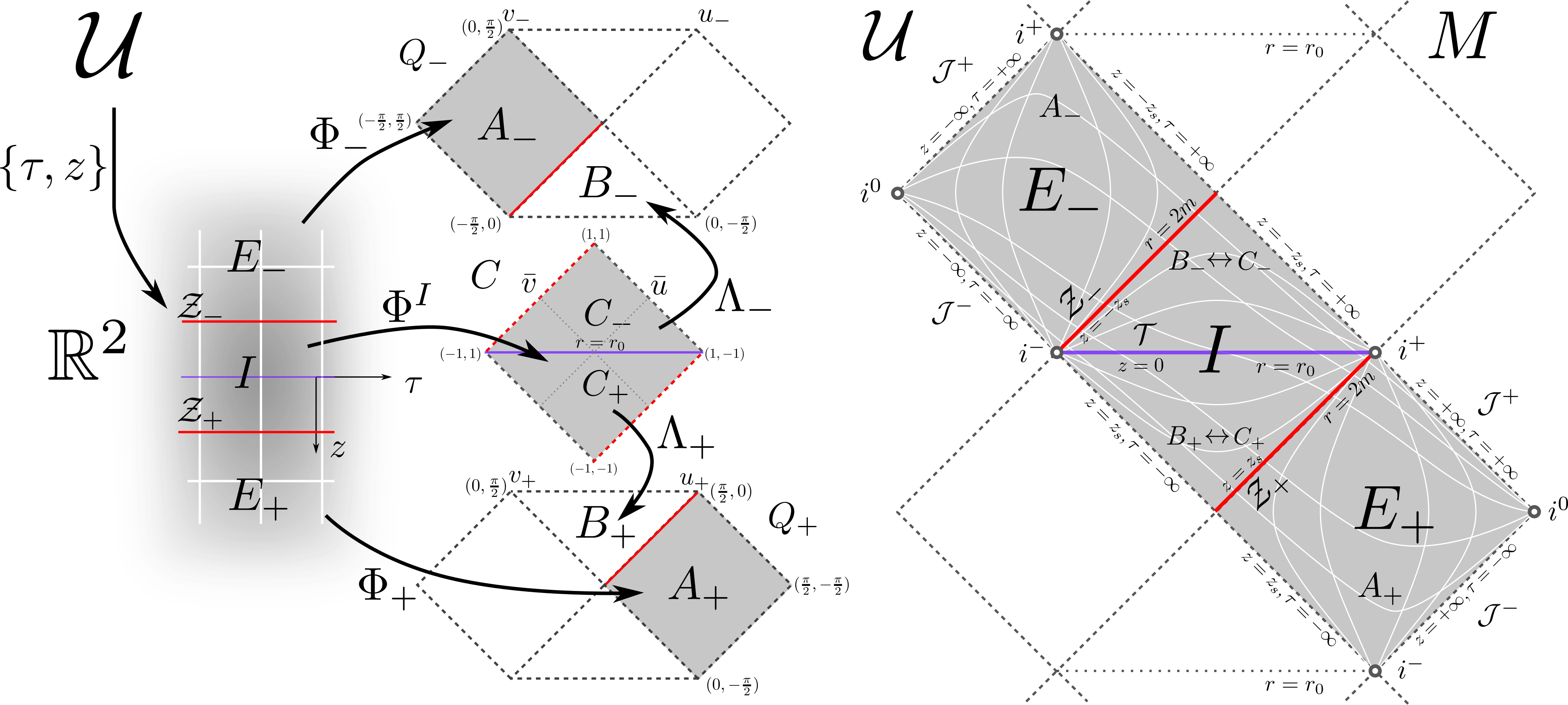
Figure 1: Penrose diagram of the domain $(\mathcal{U},g)$ (shaded) and its maximal analytical extension $(M,g)$ (outlined). We depict the diffeomorphisms that map the two exterior regions $E_{\sigma}$ and the interior region $I$, from the corresponding restrictions of the common chart $\{\tau,z\}$, to the sets $A_{\sigma}$ in the charts $\{u_{\sigma},v_{\sigma}\}$ and $C$ in the chart $\{\bar{u},\bar{v}\}$, respectively.

We first define the sets: $E:=\{r>2m\}\cap\mathcal{U}$, $I:=\{r<2m\}\cap\mathcal{U}$, $\mathcal{Z}:=\{r=2m\}\cap\mathcal{U}$, and $\mathcal{T}:=\{r=r_{0}\}\cap\mathcal{U}\subset I$. Then we use the chart $\{\tau,z\}$ to decompose these sets (except $\mathcal{T}$) by taking their restrictions under the sign function $\operatorname{sgn}(z)$, and use the notation $D_{\sigma}:=D|_{\operatorname{sgn}(z)=\sigma}$ (with $\sigma=\pm 1$) for any domain $D$. In particular, $E=E_{-}\cup E_{+}$ is disconnected and $I=I_{-}\cup\mathcal{T}\cup I_{+}$ is a connected set. To ease the notation we will use the same letter for the domain in $\mathcal{U}$ and its image on $\mathbb{R}^{2}$ under the chart $\{\tau,z\}$. For instance, $E_{+}$ also stands for the half plane $z\in(z_{s},\infty)$ in $\mathbb{R}^{2}$, where $z_{s}$ is the positive root of $r(z_{s})=2m$, and $I$ is also the stripe $z\in(-z_{s},z_{s})$.

With the auxiliary $\alpha:=4m(1-\frac{r_{0}}{2m})^{-1/2}$, $\varepsilon\!=\!\pm 1$ and

$$R_{\varepsilon}(r):=\alpha\log\left(\sqrt{r_{0}}\frac{\left|\sqrt{r-r_{0}}+\varepsilon\sqrt{2m-r_{0}}\right|}{\sqrt{2m}\sqrt{r-r_{0}}+\sqrt{r}\sqrt{2m-r_{0}}}\right)$$

$$+\left(\sqrt{r}-\varepsilon\sqrt{8m}\right)\!\sqrt{r-r_{0}}+\!(4m\!+\!r_{0})\!\log\!\left[\!\sqrt{\frac{r}{r_{0}}}\!+\!\sqrt{\frac{r}{r_{0}}-1}\right]$$

we construct $R_{U}(r):=R_{+}(r)$, $R^{E}_{V}(r):=R_{-}(r)|_{r>2m}$ and $R^{I}_{V}(r):=R_{-}(r)|_{r<2m}$. Since $R_{U}(r_{0})=0$, it is easy to check that $U(\tau,z):=\tau+\operatorname{sgn}(z)R_{U}(r(z))$ is analytic on the whole plane.

Let us first work out the causal structure of the exterior regions $E_{\sigma}$. On each $E_{\sigma}$ we define the respective function $V_{\sigma}(\tau,z)=\tau-\sigma R^{E}_{V}(r(z))$, analytic on its domain, and use $U_{\sigma}:=U|_{\operatorname{sgn}(z)=\sigma}$ to construct the diffeomorphisms $\Phi_{\sigma}:\{\tau,z\}|_{E_{\sigma}}\!\to\!\{u_{\sigma},v_{\sigma}\}$ by

$$u_{\sigma}=\sigma\arctan\exp\left[\frac{\sigma}{\alpha}U_{\sigma}(\tau,z)\right],$$

$$v_{\sigma}=-\sigma\arctan\exp\left[-\frac{\sigma}{\alpha}V_{\sigma}(\tau,z)\right],$$

that map, respectively, the domains $E_{+}$ and $E_{-}$ to the regions $A_{+}=\{u_{+}\in(0,\pi/2),v_{+}\in(-\pi/2,0)\}$ and $A_{-}=\{u_{-}\in(-\pi/2,0),v_{-}\in(0,\pi/2)\}$. In the charts $\{u_{\sigma},v_{\sigma}\}$ the metric, c.f. (9), reads

$$ds^{2}=\frac{\Gamma(r(u_{\sigma},v_{\sigma}))}{\cos^{2}u_{\sigma}\cos^{2}v_{\sigma}}du_{\sigma}dv_{\sigma}+r(u_{\sigma},v_{\sigma})^{2}d\Omega^{2},$$ (10)

with

$$\Gamma(r)\!:=\!-\frac{2m\alpha^{2}}{r}\!\left(\!\!\sqrt{1\!-\!\frac{r_{0}}{r}}\!+\!\sqrt{1\!-\!\frac{r_{0}}{2m}}\,\right)^{\!\!2}\!\!\exp\!\left[-\frac{2r}{\alpha}\sqrt{1\!-\!\frac{r_{0}}{r}}\,\right]\quad\mbox{}$$

$$\times\!\!\left(\!1\!+\!\sqrt{1\!-\!\frac{r_{0}}{r}}\right)^{\!\!-\!\sqrt{1-\frac{r_{0}}{2m}}(2+\frac{r_{0}}{2m})}\!\!\!\left(\frac{r_{0}}{r}\right)^{\!\!\sqrt{1-\frac{r_{0}}{2m}}(1+\frac{r_{0}}{4m})-1}\!\!,\!\!$$ (11)

and $r(u_{\sigma},v_{\sigma})$ satisfies

$$\tan u_{\sigma}\tan v_{\sigma}=\left(1-\frac{2m}{r}\right)\frac{\alpha^{2}}{\Gamma(r)}=:\Upsilon(r).$$ (12)

$\Gamma(r)$, as defined, is finite and negative on $r\in[r_{0},\infty)$ and satisfies $\Gamma(r)\Upsilon^{\prime}(r)=2\alpha(1-r_{0}/r)^{-1/2}$. Hence, $\Upsilon$ is a strictly decreasing function of $r$ with $\Upsilon(r_{0})=1$ and $\Upsilon(2m)=0$. For each $E_{\sigma}$ the set $A_{\sigma}$ thus provides the usual Penrose diagram for the Schwarzschild exterior. Moreover, on each $E_{\sigma}$ the change $\{\tau,z\}|_{E_{\sigma}}\!\to\!\{\tilde{t},\tilde{r}\}$, given by $\tilde{r}=r(z)$ and $\tilde{t}=\tau+\frac{\sigma}{2}\left(R_{U}(r(z))-R^{E}_{V}(r(z))\right)$, produces a chart in which the metric, c.f. (9), reads as (5). This shows $\mathcal{U}$ covers two exterior regions isometric to (a).

We proceed similarly for the interior region $I$. First, we define $V^{I}(\tau,z):=-\tau+\operatorname{sgn}(z)R^{I}_{V}(r(z))$, which is analytic in $z\in(-z_{s},z_{s})$ (note that $R^{I}_{V}(r_{0})=0$), and $U^{I}:=U|_{I}$. It can be checked that $R_{U}(r)+R^{I}_{V}(r)<0$ for $r\in(r_{0},2m)$, and therefore $\operatorname{sgn}(U^{I}+V^{I})=-\operatorname{sgn}(z)$. The diffeomorphism $\Phi^{I}:\{\tau,z\}|_{I}\to\{\bar{u},\bar{v}\}$

$$\bar{u}=\tanh\left[\frac{1}{2\alpha}U^{I}(\tau,z)\right],\quad\bar{v}=\tanh\left[\frac{1}{2\alpha}V^{I}(\tau,z)\right],$$

maps $I$ to $C=\{\bar{u}\in(-1,1),\bar{v}\in(-1,1)\}$. In this chart the metric, c.f. (9), reads

$$\!\!\!ds^{2}\!=\!{\left(\!1\!-\!\frac{2m}{r(\bar{u},\bar{v})}\!\right)\!\frac{\alpha^{2}}{(1\!-\!\bar{u}^{2})(1\!-\!\bar{v}^{2})}}d\bar{u}d\bar{v}+r(\bar{u},\bar{v})^{2}d\Omega^{2}\!,$$ (13)

where $r(\bar{u},\bar{v})$ satisfies

$$-\left|\frac{\bar{u}+\bar{v}}{1+\bar{u}\bar{v}}\right|=\tanh\left[\frac{1}{2\alpha}(R_{U}(r)+R^{I}_{V}(r))\right].$$

Since $R_{U}(r_{0})=R^{I}_{V}(r_{0})=0$ the curve $r=r_{0}$ is mapped to the horizontal line $\bar{u}+\bar{v}=0$. Further, we have $\operatorname{sgn}(U^{I}+V^{I})=\operatorname{sgn}(\bar{u}+\bar{v})$ and hence $\operatorname{sgn}(\bar{u}+\bar{v})=-\operatorname{sgn}(z)$. Therefore, each set of constant $r\in(r_{0},2m)$ corresponds to two curves of constant $(\bar{u}+\bar{v})/(1+\bar{u}\bar{v})$ that go from $(\bar{u},\bar{v})=(-1,1)$ to $(\bar{u},\bar{v})=(1,-1)$ through positive (negative) values of $\bar{u}+\bar{v}$ for $\operatorname{sgn}(z)=-1$ ($\operatorname{sgn}(z)=1$). For finite $\tau$, as $r\to 2m$, the function $R_{U}$ remains bounded whereas $R^{I}_{V}\to-\infty$. Hence points approaching $\mathcal{Z}_{\sigma}$ from $I$ attain $\bar{v}\to-\operatorname{sgn}(z)$, while $\bar{u}$ runs over its whole range. The set $C$ provides the Penrose diagram for $I$. The change $\{\tau,z\}|_{I}\to\{\overline{T},\overline{Y}\}$ defined by $\tau=\overline{Y}-\frac{\operatorname{sgn}(z)}{2}\left(R_{U}(\bar{r}(\overline{T}))-R^{I}_{V}(\bar{r}(\overline{T}))\right)$ and $\bar{r}(\overline{T})=r(z)$, that imply $\operatorname{sgn}(z)=\operatorname{sgn}(\cos\overline{T})$ and is explicitly given by

$$\tau= \overline{Y}-\alpha\,\mbox{artanh}\left[\sqrt{\frac{\bar{r}(\overline{T})}{2m}}\cos\overline{T}\right]+\frac{16m^{2}}{\alpha}\sqrt{\frac{\bar{r}(\overline{T})}{2m}}\cos\overline{T},$$

$$z= r_{0}\,\mbox{artanh}\left[\frac{4m}{\alpha}\cos\overline{T}\right]+\frac{\alpha}{8m^{2}}\bar{r}(\overline{T})\cos\overline{T}$$

with $\eqref{r_T}$, is one-to-one and takes (9) to the form (7). This shows that $I\subset\mathcal{U}$ is isometric to the region (c). Observe that $z=z_{s}$, i.e. $\mathcal{Z}_{+}$, is recovered for $\overline{T}=0$; $z=-z_{s}$, i.e. $\mathcal{Z}_{-}$, for $\overline{T}=\pi$; and $z=0$, that is $\mathcal{T}$, for $\overline{T}=\pi/2$. Further, on each $I_{\sigma}$, the change $\{\tau,z\}|_{I_{\sigma}}\to\{T,Y\}$, given by $T=r(z)$ and $Y=\tau+\frac{\sigma}{2}\left(R_{U}(r(z))-R^{I}_{V}(r(z))\right)$, renders the metric, c.f. (9), in the form (6). Therefore $I$, and thus also the region (c), cover two regions (b).

Finally, we use that $\Upsilon(r)$ strictly decreases on $[r_{0},\infty)$ with maximum $\Upsilon(r_{0})=1$, ensuring (12) has a solution for $r$ everywhere on $\tan u_{\sigma}\tan v_{\sigma}\leq 1$. Therefore each set $A_{\sigma}$ can be extended to the Kruskal-Szekeres-type regions $Q_{\sigma}$ (see Fig. 1). The purpose of these extensions is twofold. Firstly, the sets $C_{\sigma}$ can be mapped respectively to $B_{+}:=\{u_{+},v_{+}\in\!(0,\pi/2);u_{+}\!+\!v_{+}<\pi/2\}\subset Q_{+}$ and $B_{-}:=\{u_{-},v_{-}\in\!(-\pi/2,0);u_{-}\!+\!v_{-}\!>\!-\pi/2\}\subset Q_{-}$ with the diffeomorphisms $\Lambda_{\sigma}:C_{\sigma}\to B_{\sigma}$

$$u_{\sigma}=\sigma\arctan\left(\frac{1+\bar{u}_{\sigma}}{1-\bar{u}_{\sigma}}\right)^{\sigma},v_{\sigma}=\sigma\arctan\left(\frac{1+\bar{v}_{\sigma}}{1-\bar{v}_{\sigma}}\right)^{\sigma},$$

in order to define the extended charts $\{u_{\sigma},v_{\sigma}\}_{Q_{\sigma}}$ so that they map all $p\in I_{\sigma}$ by $\Lambda_{\sigma}\circ\Phi^{I}(p)$ to the respective point on $B_{\sigma}$. This ends the contruction of the full Penrose diagram for $(\mathcal{U},g)$. Secondly, we extend $(\mathcal{U},g)$ to two Kruskal-Szekeres-type analytic regions, $Q_{+}$ and $Q_{-}$, by adding their remaining halfs. These can be used to build up the maximal analytic extension of $M$ in the usual periodic fashion, and show that $M$ is geodesically complete [27].

All test particles that cross the horizon at $r=2m$, arrive to $r_{0}$, continue towards negative values of $z$ with increasing values of $r$, and cross again $r=2m$ after a finite proper time. In particular, radial infalling particles at rest at infinity take a time $\frac{8}{3}(m+r_{0})(1-\frac{r_{0}}{2m})^{1/2}$ to cross the interior region. The singularity in Schwarzschild, at $r=r_{0}=0$, is not present here and the curvature is bounded. In particular, the curvature scalars take their maximum value at $r=r_{0}$. For instance, the Ricci scalar $R=3mr_{0}/r^{4}$ is everywhere positive. Note that even if quantum-gravity effects (parametrized by $r_{0}$) are present outside the horizon, they decay as one moves to low-curvature regions.

The computation of the expansions of ingoing and outgoing radial null congruences shows, as expected, that the spheres of constant $t$ and $x$ are non-trapped in the exterior region $r>2m$, and that $r=2m$ is indeed a horizon. Moreover, in the interior region $r_{0}<r<2m$ both expansions have the same sign, given by $-\operatorname{sgn}(z)$, and vanish at $r=r_{0}$. Therefore, in $I_{+}$ ($I_{-}$) those spheres are trapped (anti-trapped) while in $\mathcal{T}$, they have zero mean curvature. In fact, the hypersurface $r=r_{0}$ itself is minimal, reflecting the mirror symmetry $z\to-z$.

Therefore, as one expects for a singularity resolution, some of the eigenvalues of the Einstein tensor ${G^{a}}_{b}$ must attain negative values on $I$. Indeed, if one interprets $G^{a}{}_{b}$ as an effective energy-momentum tensor, the eigenvalues on the angular part would define an angular pressure $(r-m)r_{0}/(2r^{4})$. On $E$ one would get a positive energy density $2mr_{0}/r^{4}$ and a negative radial pressure $-r_{0}/r^{3}$, while on $I$ the energy density would be $r_{0}/r^{3}$ and the radial pressure $-2mr_{0}/r^{4}$. With these values it is easy to check that none of the geometric energy conditions are satisfied at any point except at the horizon. However, let us recall that $(M,g)$ solves the vacuum equations, thus satisfying trivially all the physical energy conditions.

Let us finally summarize the main features of this effective quantum black-hole model: $(i)$ The brackets between deformed constraints vanish on-shell and thus form an anomaly-free algebra. $(ii)$ We provide a consistent, hence covariant, geometric setup so we can talk of a metric that solves the system. Different gauge choices on the phase space simply provide different charts (and domains) of some spacetime $(M,g)$, with corresponding expressions for the same metric tensor. $(iii)$ A convenient choice of gauge provides a single chart that covers a domain $(\mathcal{U},g)$ with global structure shown in Fig. 1, which represents a globally hyperbolic interior (black-hole/white-hole) region and two asymptotically flat exteriors of equal mass. $(iv)$ We have produced the maximal analytical extension $(M,g)$. $(v)$ Quantum-gravity effects introduce a length scale $r_{0}>0$, that defines a minimum of the area of the orbits of the spherical symmetry, and removes the classical singularity. More precisely, the surface $r=r_{0}$ is just a minimal hypersurface between a trapped and anti-trapped region, and all causal geodesics cross it in finite time. $(vi)$ All curvature scalars are bounded everywhere. $(vii)$ Quantum-gravity effects die off as we move to low-curvature regions. $(viii)$ Schwarzschild is recovered for $r_{0}=0$ and Minkowki for $m=0$.

Acknowledgments We acknowledge financial support from the Basque Government Grant No. IT956-16 and from the Grant FIS2017-85076-P, funded by MCIN/AEI/10.13039/ 501100011033 and by “ERDF A way of making Europe”. AAB is funded by the FPI fellowship PRE2018-086516 of the Spanish MCIN.