IDCAIS: Inter-Defender Collision-Aware Interception Strategy against Multiple Attackers

Abstract

In the prior literature on multi-agent area defense games, the assignments of the defenders to the attackers are done based on a cost metric associated only with the interception of the attackers. In contrast to that, this paper presents an Inter-Defender Collision-Aware Interception Strategy (IDCAIS) for defenders to intercept attackers in order to defend a protected area, such that the defender-to-attacker assignment protocol not only takes into account an interception-related cost but also takes into account any possible future collisions among the defenders on their optimal interception trajectories. In particular, in this paper, the defenders are assigned to intercept attackers using a mixed-integer quadratic program (MIQP) that: 1) minimizes the sum of times taken by defenders to capture the attackers under time-optimal control, as well as 2) helps eliminate or delay possible future collisions among the defenders on the optimal trajectories. To prevent inevitable collisions on optimal trajectories or collisions arising due to time-sub-optimal behavior by the attackers, a minimally augmented control using exponential control barrier function (ECBF) is also provided. Simulations show the efficacy of the approach.

Index Terms— cooperative robots, defense games, multi robots systems and optimal control.

I Introduction

I-1 Motivation

Various cooperative techniques are used in [1, 2, 3, 4, 5, 6, 7, 8, 9, 10, 11] for a team of defenders to effectively capture multiple attackers in order to defend a safety-critical area. However, none of these studies considers collision among the defenders on their optimal interception trajectories while making assignment of the defenders to the attackers. The possible collisions among the defenders on their optimal trajectories become particularly important when there is a possibility of such collisions, for example on non-straight optimal interception trajectories obtained in case of high order system dynamics, and when the defenders survival is to be ensured. In this paper, we develop a collaborative defense strategy for a team of defenders to intercept as many of the attackers as possible before the attackers reach the protected area, while making assignment of the defenders to the attackers that take into possible future collisions among the defenders on their optimal interception trajectories.

I-2 Related work

The area or target defense problem involving one attacking player and one defending player (i.e., 1-vs-1 area defense game) has been studied in the literature as a zero-sum differential game using various solution techniques including optimal control [1, 2, 3, 4, 5, 12, 13], reachability analysis [6], semi-definite programming [14], second-order cone programming [15], and model predictive control (MPC) [16, 17, 18].

Due to the curse of dimensionality, these approaches for 1-vs-1 area defense games are extended to multi-player scenarios using a “divide and conquer” approach. In the “divide and conquer” approach, for a given multiplayer scenario, all possible 1-vs-1 games between the defenders and the attackers are solved first. Next, the individual defenders are then assigned to capture/intercept/pursue individual attackers by solving a collaborative assignment problem based on the performance of the individual defenders against individual attackers characterized through the solutions of the solved 1-vs-1 games.

In [8], the authors solve the reach-avoid game for each pair of defenders and attackers operating in a compact domain with obstacles using a Hamilton-Jacobi-Issacs (HJI) reachability approach. The solution is then used to assign defenders against the attackers in multiplayer case using graph-theoretic maximum matching. The authors in [7] develop a distributed algorithm for the cooperative pursuit of multiple evaders by multiple pursuers, using an area-minimization strategy based on a Voronoi tessellation in a bounded convex environment. Each defender targets it nearest evader and cooperate with other neighboring pursuers who share the same evader in order to capture all the evaders in finite time.

The “divide and conquer” approach sometime may also involve solving games between sub-teams of the defending and attacking team and then making defenders to attackers assignment based on the solutions to these smaller problems. For example, in the perimeter defense problem, a variant of multi-player reach-avoid game, studied in [9], defenders are restricted to move on the perimeter of protected area. Local reach-avoid games between small teams of defenders and attackers are first solved, and then the defenders or teams of defenders are assigned to capture the oncoming attackers using a polynomial-time algorithm. In [19] the authors consider a multi-player reach-avoid game in 3D with heterogeneous players. The authors first decompose the original multi-player game into multiple smaller games involving coalitions of three or less pursuers and only one evader, using a HJI formulation. Then a sequential matching problem is solved on a conflict graph with pursuers’ coalitions and evaders as the nodes in order to find an approximate assignment that assigns the coalitions of pursuers to capture the evaders.

The aforementioned studies provide useful insights to the area or target defense problem, however, are limited in application due to the use of the single-integrator motion model, and due to the lack of consideration of inter-defender collisions. In [10], the authors consider a Target-Attacker-Defender (TAD) game with agents moving under double-integrator dynamics, and use the isochrones method to design time-optimal control strategies for the players. In [11], the authors develop a time-optimal strategy for a Dubins vehicle to intercept a target moving with constant velocity, an assumption that could be limiting in practice. However, both of these approaches lack consideration of collisions among the defenders that may happen on the defenders’ optimal interception trajectories.

I-3 Overview and summary of our contributions

In this paper, we resort to the common “divide and conquer” paradigm and provide a collaborative interception strategy for the defenders that takes into account any possible future collisions among the defenders on their optimal interception trajectories at the defender-to-attacker assignment stage. We build on the time-optimal guidance problem for isotropic rocket [20], which uses a damped double-integrator motion model, and formulate a non-zero sum game between each pair of defender and attacker to obtain a time-optimal strategy for a defender to capture a given attacker. We then use the times of interception by each defender to capture each attacker, and the times of possible collisions on the defenders’ optimal trajectories, to assign the defenders to the attackers. We call this assignment the collision-aware defender-to-attacker assignment (CADAA). Furthermore, we use exponential control barrier functions (ECBF) [21, 22] in a quadratically constrained quadratic program (QCQP) to augment defenders’ optimal control actions in order to avoid collision with other fellow defenders when such collisions are unavoidable solely by CADAA. The overall defense strategy that combines CADAA and ECBF-QCQP is called as inter-defender collision-aware interception strategy (IDCAIS).

This is the first time a defender-attacker assignment framework is presented that considers possible future collisions among the defenders on their optimal interception trajectories. In summary, the major contributions of this paper compared to the prior literature are: (1) a non-zero-sum game between a defender and an attacker to obtain a time-optimal defense strategy, and (2) a mixed-integer quadratic program (MIQP) to find collision-aware assignment CADAA in order to capture as many attackers as possible and as quickly as possible, while preventing or delaying the possible future collisions among the defenders, and 3) a heuristic to quickly find future collision times on defenders’ optimal trajectories.

I-4 Organization

Section II provides the problem statement. The interception strategy for the 1-defender-vs-1-attacker area defense game is given in Section III, and that for multiple defenders vs multiple attackers is discussed in Section IV. Simulation results and conclusions are given in Section V and Section VI, respectively.

II Modeling and Problem Statement

Notation: $\left\lVert\cdot\right\rVert$ denotes the Euclidean norm of its argument. $\left|\cdot\right|$ denotes absolute value of a scalar argument and cardinality if the argument is a set. An open ball of radius $\rho$ centered at the origin is defined as $\mathcal{B}_{\rho}=\{\mathbf{r}\in\mathbb{R}^{2}|\left\lVert\mathbf{r}\right\rVert<\rho\}$ and that centered at $\mathbf{r}_{c}$ is defined $\mathcal{B}_{\rho}(\mathbf{r}_{c})=\{\mathbf{r}\in\mathbb{R}^{2}|\left\lVert\mathbf{r}-\mathbf{r}_{c}\right\rVert\leq\rho\}$. $A\backslash B$ denotes all the elements of the set $A$ that are not in the set $B$. We define $C(\theta)=\cos(\theta)$, $S(\theta)=\sin(\theta)$.

We consider $N_{a}$ attackers denoted as $\mathcal{A}_{i}$, $i\in I_{a}=\{1,2,...,N_{a}\}$, and $N_{d}$ defenders denoted as $\mathcal{D}_{j}$, $j\in I_{d}=\{1,2,...,N_{d}\}$, operating in a 2D environment $\mathcal{W}\subseteq\mathbb{R}^{2}$ that contains a circular protected area $\mathcal{P}\subset\mathcal{W}$, defined as $\mathcal{P}=\{\textbf{r}\in\mathbb{R}^{2}\;|\;\left\lVert\textbf{r}-\textbf{r}_{p}\right\rVert\leq\rho_{p}\}$. The number of defenders is no less than that of attackers, i.e., $N_{d}\geq N_{a}$. The agents $\mathcal{A}_{i}$ and $\mathcal{D}_{j}$ are modeled as discs of radii $\rho_{a}$ and $\rho_{d}(\leq\rho_{a})$, respectively.

Figure 1: Problem Formulation

Let $\mathbf{r}_{ai}=[x_{ai}\;y_{ai}]^{T}$ and $\mathbf{r}_{dj}=[x_{dj}\;y_{dj}]^{T}$ be the position vectors of $\mathcal{A}_{i}$ and $\mathcal{D}_{j}$, respectively; $\mathbf{v}_{ai}=[v_{x_{ai}}\;v_{y_{ai}}]^{T}$, $\mathbf{v}_{dj}=[v_{x_{dj}}\;v_{y_{dj}}]^{T}$ be the velocity vectors, respectively, and $\mathbf{u}_{ai}=[u_{x_{ai}}\;u_{y_{ai}}]^{T}$, $\mathbf{u}_{dj}=[u_{x_{dj}}\;u_{y_{dj}}]^{T}$ be the accelerations, which serve also as the control inputs, respectively, all resolved in a global inertial frame $\mathcal{F}_{gi}(\hat{\mathbf{i}},\hat{\mathbf{j}})$ (see Figure1). The agents move under double integrator (DI) dynamics with linear drag (damped double integrator), similar to isotropic rocket [20]:

$$\dot{\mathbf{x}}_{\imath}=\begin{bmatrix}\dot{\mathbf{r}}_{\imath}\\ \dot{\mathbf{v}}_{\imath}\end{bmatrix}=\underbrace{\begin{bmatrix}\mathbf{0}_{2}&\mathbf{I}_{2}\\ \mathbf{0}_{2}&-C_{D}\mathbf{I}_{2}\end{bmatrix}}_{\mathbf{A}}\mathbf{x}_{\imath}+\underbrace{\begin{bmatrix}\mathbf{0}_{2}\\ \mathbf{I}_{2}\end{bmatrix}}_{\mathbf{B}}\mathbf{u}_{\imath},$$ (1)

where ${\imath}\in\{ai\;|\;i\in I_{a}\}\cup\{dj\;|\;j\in I_{d}\}$ (with $ai$ denoting the $i^{th}$ attacker $\mathcal{A}_{i}$ and $dj$ denoting the $j^{th}$ defender $\mathcal{D}_{j}$), $C_{D}>0$ is the known, constant drag coefficient. The accelerations $\mathbf{u}_{ai}$ and $\mathbf{u}_{dj}$ are bounded by $\bar{u}_{a}$, $\bar{u}_{d}$ as: $\left\lVert\mathbf{u}_{ai}\right\rVert\leq\bar{u}_{a},\quad\left\lVert\mathbf{u}_{dj}\right\rVert\leq\bar{u}_{d},$ By incorporating the drag term, the damped double integrator (1) inherently poses a speed bound on each agent under a limited acceleration control, i.e.,

$$\left\lVert\mathbf{v}_{ai}\right\rVert<\bar{v}_{a}=\frac{\bar{u}_{a}}{C_{D}}\text{ and }\left\lVert\mathbf{v}_{dj}\right\rVert<\bar{v}_{d}=\frac{\bar{u}_{d}}{C_{D}},$$ (2)

and does not require an explicit constraint on the velocity of the agents while designing bounded controllers, as in earlier literature. So we have $\mathbf{x}_{ai}\in\mathcal{X}_{a}$, for all $i\in I_{a}$, where $\mathcal{X}_{a}=\mathbb{R}^{2}\times\mathcal{B}_{\bar{v}_{a}}$ and $\mathbf{x}_{dj}\in\mathcal{X}_{d}$, for all $j\in I_{d}$, where $\mathcal{X}_{d}=\mathbb{R}^{2}\times\mathcal{B}_{\bar{v}_{d}}$. We denote by $\mathcal{X}=\mathcal{X}_{a}^{N_{a}}\times\mathcal{X}_{d}^{N_{d}}$ the configuration space of all the agents. We also make the following assumptions:

Assumption 1

The defenders are assumed to be at least as fast as the attackers, i.e., $\bar{u}_{a}\leq\bar{u}_{d}$.

Note that under Assumption 1, and by virtue of eq. (2), the maximum velocities of the attackers and defenders also satisfy $\bar{v}_{a}\leq\bar{v}_{d}$.

Assumption 2

Each player (either defender or attacker) knows the states of the all the other players.

Each defender $\mathcal{D}_{j}$ is endowed with an interception radius $\rho_{d}^{int}$, i.e., the defender $\mathcal{D}_{j}$ is able to physically damage an attacker $\mathcal{A}_{i}$ when $\left\lVert\mathbf{r}_{dj}-\mathbf{r}_{ai}\right\rVert<\rho_{d}^{int}$.

The goal of the attackers is to as many of them reach the protected area $\mathcal{P}$. The defenders aim to capture these attackers before they reach the protected area $\mathcal{P}$, while ensuring they themselves do not collide with each other. Formally, we consider the following problem.

Problem 1 (Collision-Aware Multi-player Defense)

Design a control strategy $\mathbf{u}_{dj}$ for the defenders $\mathcal{D}_{j}$, $\forall j\in I_{d}$ to: 1) intercept as many attackers and as quickly as possible before the attackers reach the protected area $\mathcal{P}$, 2) ensure that the defenders do not collide with each other, i.e., $\left\lVert\mathbf{r}_{dj}(t)-\mathbf{r}_{dj^{\prime}}(t)\right\rVert>\rho_{d}^{col}$ for all $j,j^{\prime}\neq j\in I_{d}$ for all $t\geq 0$.

Before discussing the solution to Problem 1, we discuss the one defender against one attacker game as follows.

III Interception strategy: one defender against one attacker

In this section, we first consider a scenario with one attacker attacking the protected area $\mathcal{P}$ and one defender trying to defend $\mathcal{P}$ by intercepting the attacker (1D-vs-1A game). The solution to these one-on-one games is then used later to solve Problem 1. We consider a time-optimal control strategy for the defender. Before we discuss this strategy, we first discuss time-optimal control for an agent moving under (1) in the following subsection.

III-1 Time-optimal control under damped double integrator

The time-optimal control problem for an agent starting at $\mathbf{x}_{\imath 0}=[x_{\imath 0},y_{\imath 0},v_{x_{\imath 0}},v_{y_{\imath 0}}]^{T}$ and moving under (1) to reach the origin $[0,0]^{T}$, is formally defined as:

$$\mathbf{u}_{\imath}^{*}(t)=\displaystyle\operatorname*{arg\,min}_{\mathbf{u}_{\imath}(t)}\hskip 5.69054pt J(\mathbf{u}(t))=\int_{0}^{t_{f}}dt$$ (3a)

subject to $$1)\;\dot{\mathbf{x}}_{\imath}(t)={\mathbf{A}}\mathbf{x}_{\imath}(t)+{\mathbf{B}}\mathbf{u}_{\imath}(t),$$ (3b)

$$2)\;\left\lVert\mathbf{u}_{\imath}(t)\right\rVert\leq\bar{u},$$ (3c)

$$3)\;\mathbf{x}_{\imath}(0)=\mathbf{x}_{\imath 0},$$ (3d)

$$4)\;\mathbf{r}_{\imath}(t_{f})=[0,0]^{T},$$ (3e)

where $t_{f}$ is free terminal time at which $\mathbf{r}_{\imath}(t_{f})=[0,0]^{T}$. After invoking Pontryagin’s minimum principle [23], the optimal control $\mathbf{u}_{\imath}^{*}(t)$ solving (3) is given by:

$$\begin{array}[]{ll}\mathbf{u}_{\imath}^{*}(t)=\bar{u}\big{[}\frac{-\lambda_{3}^{*}(t)}{\sqrt{(\lambda_{3}^{*}(t))^{2}+(\lambda_{4}^{*}(t))^{2}}},\frac{-\lambda_{4}^{*}(t)}{\sqrt{(\lambda_{3}^{*}(t))^{2}+(\lambda_{4}^{*}(t))^{2}}}\big{]}^{T}\end{array}$$ (4)

where $\bm{\lambda}^{*}(t)=[\lambda_{1}^{*}(t),\;\lambda_{2}^{*}(t),\;\lambda_{3}*(t),\;\lambda_{4}^{*}(t)]^{T}=\begin{bmatrix}c_{1},\hskip 7.11317ptc_{2},\hskip 7.11317ptc_{1}-c_{3}e^{-C_{D}t},\hskip 7.11317ptc_{2}-c_{4}e^{-C_{D}t}\end{bmatrix}^{T}$ is the co-state vector, where $c_{i}$ for $i\in\{1,2,3,4\}$ are some constants that depend on the boundary conditions in (3). Similar to the time-optimal control for simple double integrator dynamics [10, 24], the optimal control $\mathbf{u}_{\imath}^{*}(t)$ in (4) is a constant vector for all $t\in[0,t_{f}]$ as shown in Proposition 3.2 in [20]. One can write $\mathbf{u}_{\imath}^{*}(t)=\bar{u}[C(\theta_{\imath}^{*}),\;S(\theta_{\imath}^{*})]^{T}$, where $\theta_{\imath}^{*}$ is the angle made by the vector $\mathbf{u}_{\imath}^{*}(t)$ with the $x$-axis.

After integrating the system dynamics (1) under the constant input $\mathbf{u}_{\imath}^{*}(t)$, the position trajectories are obtained as follows:

$$\begin{array}[]{ll}x_{\imath}^{*}(t)=x_{\imath 0}+E_{1}(t)v_{x_{\imath 0}}+E_{2}(t)\bar{u}C(\theta_{\imath}^{*}),\\ y_{\imath}^{*}(t)=y_{\imath 0}+E_{1}(t)v_{y_{\imath 0}}+E_{2}(t)\bar{u}S(\theta_{\imath}^{*}).\end{array}$$ (5)

where $E_{1}(t)=\frac{1-e^{-C_{D}t}}{C_{D}}$ and $E_{2}(t)=\frac{t-E_{1}(t)}{C_{D}}$. By using the terminal constraint from (3e) in eq. (5), the optimal control $\mathbf{u}_{\imath}^{*}(t)=\bar{u}[C(\theta_{\imath}^{*}),\;S(\theta_{\imath}^{*})]^{T}$ and the terminal time $t_{f}$ can be found by solving the following equations simultaneously.

$$\begin{array}[]{ll}0=x_{\imath 0}+E_{1}(t_{f})v_{x_{\imath 0}}+E_{2}(t_{f})\bar{u}C(\theta_{\imath}^{*}),\\ 0=y_{\imath 0}+E_{1}(t_{f})v_{y_{\imath 0}}+E_{2}(t_{f})\bar{u}S(\theta_{\imath}^{*}).\end{array}$$ (6)

III-2 Defender’s interception strategy against an attacker

On one hand, the attacker aims to reach the protected area as quickly as possible in order to avoid getting intercepted (captured) by the defender before reaching the protected area. On the other hand, the defender aims to intercept the attacker as quickly as possible in order to reduce the chances of the attacker reaching the protected area. These goals of the players do not necessarily translate into a zero-sum differential game, because the gain of one player is not exactly the same as the loss of the other player. This problem is better formulated as a non-zero sum game between the defender and the attacker. Furthermore, we assume that 1) neither the defender nor the attacker is aware of the objective function of the other player, and 2) no player announces their action before the other player. Due to this assumption, neither Nash strategy nor Stackelberg strategy is available. So, we develop a best-against-worst strategy for the defender against an attacker, i.e., the best strategy for the defender against the strategy of the attacker that has the worst consequences for the defender.

If the attacker is risk-taking, i.e., it does not care about its own survival, and its main goal is to damage the protected area, then the best action the attacker can take is to aim to reach the protected area in minimum time without worrying how the defender is moving. Since the defender wants to intercept the attacker before the latter reaches the protected area, the time-optimal control by the attacker has the worst consequences for the defender. This time-optimal control action for the attacker starting at $\mathbf{x}_{a0}$ is calculated by solving:

$$\mathbf{u}_{a}^{*}(t)=\operatorname*{arg\,min}_{\mathbf{u}_{a}(t)}\hskip 5.69054pt J_{a}(\mathbf{u}_{a}(t))=\int_{0}^{t_{a}^{int}}dt$$ (7a)

subject to $$1)\;\dot{\mathbf{x}}_{a}={\mathbf{A}}\mathbf{x}_{a}+{\mathbf{B}}\mathbf{u}_{a},$$ (7b)

$$2)\;\left\lVert\mathbf{u}_{a}(t)\right\rVert\leq\bar{u}_{a},$$ (7c)

$$3)\;\mathbf{x}_{a}(0)=\mathbf{x}_{a0},$$ (7d)

$$4)\;\left\lVert\mathbf{r}_{a}(t_{a}^{int})-\mathbf{r}_{p}\right\rVert=0,$$ (7e)

where $t_{a}^{int}$ is a free time that attacker requires to reach the protected area $\mathcal{P}$. The defender also employs a time-optimal control action based on the time-optimal control that the attacker may take to reach the protected area. We call this a best-against-worst strategy and is obtained by solving the following time-optimal problem for the defenders starting at $\mathbf{x}_{d0}$.

$$\mathbf{u}_{d}^{*}(t)=\displaystyle\operatorname*{arg\,min}_{\mathbf{u}_{d}(t)}\hskip 5.69054pt J_{d}(\mathbf{u}_{d}(t))=\int_{0}^{t_{d}^{int}}dt$$ (8a)

subject to $$1)\;\dot{\mathbf{e}}(t)={\mathbf{A}}\mathbf{e}(t)+{\mathbf{B}}(\mathbf{u}_{d}(t)-\mathbf{u}_{a}^{*}(t)),$$ (8b)

$$2)\;\mathbf{u}_{a}^{*}(t)\text{ is the solution of \eqref{eq:attackMinTimeProblem}},$$ (8c)

$$3)\;\left\lVert\mathbf{u}_{d}(t)\right\rVert\leq{\bar{u}_{d}^{\prime}},$$ (8d)

$$4)\;\mathbf{e}(0)=\mathbf{e}_{0},$$ (8e)

$$5)\;{\left\lVert\mathbf{e}(t_{d}^{int})\right\rVert=0},$$ (8f)

where $\mathbf{e}(t)=[e_{x}(t),e_{y}(t),e_{v_{x}}(t),e_{v_{y}}(t)]^{T}=\mathbf{x}_{d}(t)-\mathbf{x}_{a}(t)$, $t_{d}^{int}$ is the time when the defender captures the attacker and $\bar{u}_{d}^{\prime}=\bar{u}_{d}-\epsilon_{d}$ where $\epsilon_{d}$ ($\ll$ 1) is a very small, strictly positive, user-defined constant to ensure that the constraints satisfy the strict complementary slackness condition, and in turn ensure continuity of the solution to the quadratically-constrained quadratic program (QCQP) used for collision avoidance in multi-defender case discussed later in Subsection IV-A. Note that we set $\rho_{d}^{int}$ and $\rho_{a}^{int}$ to be 0 in (7) and (8) to be able to use the results from Section III-1.

Similar to (4), one can establish that the optimal controls $\mathbf{u}_{d}^{*}(t)={\bar{u}_{d}^{\prime}}[C(\theta_{d}^{*}),S(\theta_{d}^{*})]^{T}$ and $\mathbf{u}_{a}^{*}(t)=\bar{u}_{a}[C(\theta_{a}^{*}),S(\theta_{a}^{*})]^{T}$ are constant vectors. The angles $\theta_{d}^{*},\;\theta_{a}^{*},$ and the terminal times $t_{d}^{int},\;t_{a}^{int}$ can be found by solving the following set of equations:

$$\begin{array}[]{ll}x_{p}&=x_{a}+E_{1}(t_{a}^{int})v_{x_{a}}+E_{2}(t_{a}^{int})\bar{u}_{a}C(\theta_{a}^{*}),\\ y_{p}&=y_{a}+E_{1}(t_{a}^{int})v_{y_{a}}+E_{2}(t_{a}^{int})\bar{u}_{a}S(\theta_{a}^{*}),\\ 0&=e_{x}+E_{1}(t_{d}^{int})e_{v_{x}}+E_{2}(t_{d}^{int})({\bar{u}_{d}^{\prime}}C(\theta_{d}^{*})-\bar{u}_{a}C(\theta_{a}^{*})),\\ 0&=e_{y}+E_{1}(t_{d}^{int})e_{v_{y}}+E_{2}(t_{d}^{int})({\bar{u}_{d}^{\prime}}S(\theta_{d}^{*})-\bar{u}_{a}S(\theta_{a}^{*})).\end{array}$$ (9)

The defender computes the best-against-worst time-optimal strategy at every time step in order to correct its action in reaction to any time-sub-optimal behavior by the attacker. We notice that the control action $\mathbf{u}_{d}^{*}(t)$ obtained in (8) is a function of the current states of the players $\mathbf{x}_{d}$ and $\mathbf{x}_{a}$, i.e., it is a closed-loop control law. Next, we discuss winning regions of the players.

III-3 Winning regions of the players

In this section, for a given initial condition $\mathbf{x}_{d}$ of the defender, we characterize the set of initial conditions of the attacker for which the defender is able to capture the attacker under the control strategy (8). This set, called as winning region of the defender, is denoted by $\mathcal{R}_{d}(\mathbf{x}_{d})$:

$$\mathcal{R}_{d}(\mathbf{x}_{d})=\{\mathbf{x}_{a}\in\bar{\mathcal{X}}_{a}|t_{d}^{int}(\mathbf{x}_{d},\mathbf{x}_{a})-t_{a}^{int}(\mathbf{x}_{a},\mathbf{r}_{p})\leq 0\},$$ (10)

where $\bar{\mathcal{X}}_{a}=(\mathbb{R}^{2}\backslash\mathcal{P})\times\mathcal{B}_{\bar{v}_{a}}$, $t_{a}^{int}(\mathbf{x}_{a},\mathbf{r}_{p})$ is the time that the attacker starting at $\mathbf{x}_{a}$ requires to reach the protected area at $\mathbf{r}_{p}$, and $t_{d}^{int}(\mathbf{x}_{d},\mathbf{x}_{a})$ is the time that defender starting at $\mathbf{x}_{d}$ requires to capture the attacker starting at $\mathbf{x}_{a}$ under the control strategy in (9). Similarly, the winning region of the attacker, denoted as $\mathcal{R}_{a}(\mathbf{x}_{d})$, is defined as $\mathcal{R}_{a}(\mathbf{x}_{d})=\bar{\mathcal{X}}_{a}\backslash\mathcal{R}_{d}(\mathbf{x}_{d})$.

In the following theorem, we formally prove the effectiveness of the best-against-worst time-optimal strategy.

Theorem 1

Let Assumption 1 hold such that $\mathcal{A}$, i.e., $\bar{u}_{a}\leq{\bar{u}_{d}^{\prime}<\bar{u}_{d}}$. The defender $\mathcal{D}$, starting at $\mathbf{x}_{d}$, moving under the control strategy $\mathbf{u}_{d}^{*}(t)$ (from (8)) against the attacker $\mathcal{A}$ initially located in $\mathcal{R}_{d}(\mathbf{x}_{d})$: i) captures $\mathcal{A}$ before $\mathcal{A}$ reaches the protected area $\mathcal{P}$, i.e., $\left\lVert\mathbf{r}_{d}(t_{d}^{int})-\mathbf{r}_{a}(t_{d}^{int})\right\rVert$ $\leq\varrho_{d}^{int}$ and $\left\lVert\mathbf{r}_{p}-\mathbf{r}_{a}(t_{d}^{int})\right\rVert>\varrho_{a}^{int}$, if $\mathcal{A}$ applies time-optimal control (7); or ii) keeps $\mathcal{A}$ outside $\mathcal{P}$, if $\mathcal{A}$ applies any control except (7).

Proof:

i) Time-optimal trajectories by construction ensure that the defender captures the attacker whenever the attacker starts inside $\mathcal{R}_{d}(\mathbf{x}_{d})$ before the attacker reaches the protected area.

ii) For the case when attacker does not use time-optimal control, showing that $\mathcal{R}_{d}(\mathbf{x}_{d})$ is forward invariant is sufficient to prove that $\mathcal{A}$ does not reach $\mathcal{P}$ because $\mathcal{P}$ is always outside of the set $\mathcal{R}_{d}(\mathbf{x}_{d})$.

Let $\tau=t_{d}^{int}(\mathbf{x}_{d},\mathbf{x}_{a})-t_{a}^{int}(\mathbf{x}_{a},\mathbf{r}_{p})$ and the boundary $\partial\mathcal{R}_{d}(\mathbf{x}_{d})$ of $\mathcal{R}_{d}(\mathbf{x}_{d})$ be defined as:

$$\partial\mathcal{R}_{d}(\mathbf{x}_{d})=\{\mathbf{x}_{a}\in(\mathbb{R}^{2}\backslash\mathcal{P})\times\mathcal{B}_{\bar{v}_{a}}|\tau=0\}.$$ (11)

As per Nagumo’s theorem [25], the necessary and sufficient condition for forward invariance of the set $\mathcal{R}_{d}(\mathbf{x}_{d})$ is to have $\dot{\tau}\leq 0$ on the boundary $\partial\mathcal{R}_{d}(\mathbf{x}_{d})$ of $\mathcal{R}_{d}(\mathbf{x}_{d})$.

Let attacker apply a time-sub-optimal action, $\mathbf{u}_{a}=\mathbf{u}_{a}^{*}+\Delta\mathbf{u}_{a}=\bar{u}_{a}[C(\theta_{a}^{*}),S(\theta_{a}^{*}\;]^{T}+[\Delta u_{x_{a}},\Delta u_{y_{a}}]^{T}\in\mathcal{B}_{\bar{u}_{a}}$, which requires $\Delta\mathbf{u}_{a}\in\mathcal{B}_{\bar{u}_{a}}(-\mathbf{u}_{a}^{*})$. After performing some algebra on (9), we obtain:

$$\begin{array}[]{ll}\dot{\tau}&=\frac{\partial{t_{d}^{int}}}{\partial{v_{x_{a}}}}\Delta u_{x_{a}}+\frac{\partial{t_{d}^{int}}}{\partial{v_{y_{a}}}}\Delta u_{y_{a}}-(\frac{\partial{t_{a}^{int}}}{\partial{v_{x_{a}}}}\Delta u_{x_{a}}+\frac{\partial{t_{a}^{int}}}{\partial{v_{y_{a}}}}\Delta u_{y_{a}})\\ &=(\frac{\partial{t_{d}^{int}}}{\partial{v_{x_{a}}}}-\frac{\partial{t_{a}^{int}}}{\partial{v_{x_{a}}}})\Delta u_{x_{a}}+(\frac{\partial{t_{d}^{int}}}{\partial{v_{y_{a}}}}-\frac{\partial{t_{a}^{int}}}{\partial{v_{y_{a}}}})\Delta u_{y_{a}}\end{array}$$ (12)

On the boundary $\partial\mathcal{R}_{d}(\mathbf{x}_{d})$, we have:

$$\begin{array}[]{ll}\dot{\tau}&\stackrel{{\scriptstyle\eqref{eq:defender_winning_region}}}{{=}}\Bigl{(}C(\theta_{a}^{*})\frac{E_{1}(t_{d}^{int})\Gamma_{d}}{\Gamma_{a}\Gamma_{d0}}\Bigr{)}\Delta u_{x_{a}}+\Bigl{(}S(\theta_{a}^{*})\frac{E_{1}(t_{d}^{int})\Gamma_{d}}{\Gamma_{a}\Gamma_{d0}}\Bigr{)}\Delta u_{y_{a}}\\ &=\Gamma\cdot(\mathbf{u}_{a}^{*})^{T}\Delta\mathbf{u}_{a}\end{array}$$ (13)

where $\Gamma=\frac{E_{1}(t_{d}^{int})\Gamma_{d}}{\Gamma_{a}\Gamma_{d0}}$, $\Gamma_{\jmath}=e^{-C_{D}t_{\jmath}^{int}}\bigl{(}v_{x_{\jmath}}C(\theta_{\jmath}^{*})+v_{y_{\jmath}}S(\theta_{\jmath}^{*})\bigr{)}+E_{1}(t_{\jmath}^{int})\bar{u}_{\jmath}$ for $\jmath\in\{a,d\}$ and $\Gamma_{d0}=e^{-C_{D}t_{d}^{int}}\bigl{(}e_{v_{x}}C(\theta_{d}^{*})+e_{v_{y}}S(\theta_{d}^{*})\bigr{)}+E_{1}(t_{d}^{int})(\bar{u}_{d}-\bar{u}_{a}C(\theta_{d}^{*}-\theta_{a}^{*}))$. From (13), we know that the maximum value $\dot{\tau}_{max}$ of $\dot{\tau}$ subject to $\Delta\mathbf{u}_{a}\in\mathcal{B}_{\bar{u}_{a}}(-\mathbf{u}_{a}^{*})$ occurs at the intersection point $\Delta\mathbf{u}_{a}^{*}$ of the circular boundary of $\mathcal{B}_{\bar{u}_{a}}(-\mathbf{u}_{a}^{*})$ and the ray along the unit vector $\hat{\mathbf{u}}_{a}^{*}=\frac{\mathbf{u}_{a}^{*}}{\left\lVert\mathbf{u}_{a}^{*}\right\rVert}$, that originated at the center of $\mathcal{B}_{\bar{u}_{a}}(-\mathbf{u}_{a}^{*})$, which implies $\Delta\mathbf{u}_{a}^{*}=[0,0]^{T}$ (see Figure 2).

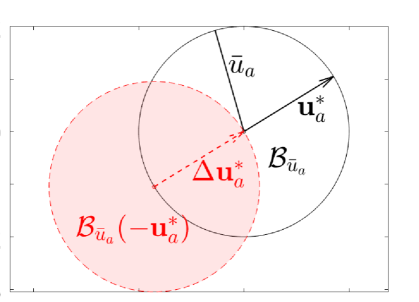
Figure 2: Control Vectors

This means $\dot{\tau}_{max}=0$ and that $\dot{\tau}\leq 0$ on the boundary $\partial\mathcal{R}_{d}(\mathbf{x}_{d})$. This implies that the set $\mathcal{R}_{d}(\mathbf{x}_{d})$ is forward invariant when attacker starts in $\mathcal{R}_{d}(\mathbf{x}_{d})$ and uses any time-sub-optimal control, and hence the attacker will not be able to reach $\mathcal{P}$ as $\mathcal{P}$ lies outside $\mathcal{R}_{d}(\mathbf{x}_{d})$. ∎

Note that since the defender is at least as fast the attacker, the attacker is unable to avoid the defender and reach protected area $\mathcal{P}$ using any time-sub-optimal behaviour. This, however, is not necessarily true when the attacker is faster than the defender; nevertheless, studying this problem is beyond the scope of this paper.

IV Collision-Aware Interception Strategy: multiple defenders against multiple attackers

To solve Problem 1, we design the defenders’ control strategy by: 1) solving each pairwise game, and 2) assigning the defenders to go against particular attackers based on a cost metric that relies on the solutions to the pairwise games, which is a common approach that many of previous works used. However, different from the earlier works, we define the assignment metric based on 1) the time-to-capture and 2) the time of possible collision between the defenders. We aim to find the assignment so that the defenders 1) intercept as many attackers as possible before they reach the protected area, and 2) ensure that defenders have minimum possible collisions among themselves. We call this collision-aware defender-to-attacker assignment (CADAA).

Let $\delta_{ji}$ be the binary decision variable that takes value 1 if the defender $\mathcal{D}_{j}$ is assigned to intercept the attacker $\mathcal{A}_{i}$ and 0 otherwise. Let $C_{d}^{int}(\mathbf{X}_{dj}^{ai})$ be the cost incurred by the defender $\mathcal{D}_{j}$ to capture the attacker $\mathcal{A}_{i}$ given by:

$$C_{d}^{int}(\mathbf{X}_{dj}^{ai})=\begin{cases}t_{d}^{int}(\mathbf{x}_{dj},\mathbf{x}_{ai}),&\text{if }\mathbf{x}_{ai}\in\mathcal{R}_{d}(\mathbf{x}_{dj});\\ {c_{l}},&\text{otherwise};\end{cases}$$ (14)

where $\mathbf{X}_{dj}^{ai}=[\mathbf{x}_{dj}^{T},\mathbf{x}_{ai}^{T}]^{T}$, $t_{d}^{int}(\mathbf{x}_{dj},\mathbf{x}_{ai})$ is the time required by the defender initially located at $\mathbf{x}_{dj}$ to capture the attacker initially located at $\mathbf{x}_{ai}$ as obtained by solving (9), $c_{l}\;(>>1)$ is a very large number, and $\mathcal{R}_{d}(\mathbf{x}_{dj})$ is the winning region of the defender initially located at $\mathbf{x}_{dj}$ defined in (10). As defined in (14), the cost $C_{d}^{int}(\mathbf{X}_{dj}^{ai})$ is set to very the large value $c_{l}$ whenever the defender is unable to capture the attacker before the attacker can reach the protected area.

Two defenders $\mathcal{D}_{j}$ and $\mathcal{D}_{j^{\prime}}$ are said to have collided with each other if $\left\lVert\mathbf{r}_{dj}(t)-\mathbf{r}_{dj^{\prime}}(t)\right\rVert<\rho_{d}^{col}$ for some $t\geq 0$, where $\rho_{d}^{col}$ is a user defined collision parameter. Consider that two defenders starting at $\mathbf{x}_{dj}$ and $\mathbf{x}_{dj^{\prime}}$ and operating under the optimal control actions obtained from (8) that corresponds to the attackers starting at $\mathbf{x}_{ai}$ and $\mathbf{x}_{ai^{\prime}}$, respectively, collide; then, let $t_{d}^{col}(\mathbf{X}_{dj}^{ai},\mathbf{X}_{dj^{\prime}}^{ai^{\prime}})$ denote the smallest time at which this collision occurs. Since the analytical expressions for optimal trajectories are known, see (9), one could easily find this time $t_{d}^{col}(\mathbf{X}_{dj}^{ai},\mathbf{X}_{dj^{\prime}}^{ai^{\prime}})$ by checking the evolution of the distance between the defenders. Let $C_{d}^{col}(\mathbf{X}_{dj}^{ai},\mathbf{X}_{dj^{\prime}}^{ai^{\prime}})$ be the cost associated with a collision that may occur between the two defenders:

$$\begin{array}[]{ll}C_{d}^{col}(\mathbf{X}_{dj}^{ai},\mathbf{X}_{dj^{\prime}}^{ai^{\prime}})=\begin{cases}\frac{1}{t_{d}^{col}(\mathbf{X}_{dj}^{ai},\mathbf{X}_{dj^{\prime}}^{ai^{\prime}})},&\text{if $\mathcal{D}_{j}$ \& $\mathcal{D}_{j^{\prime}}$ collide};\\ 0,&\text{otherwise}.\end{cases}\end{array}$$ (15)

This cost is chosen so that collisions that occur earlier are penalized more in order to delay or, if possible, avoid them. We assume that $t_{d}^{col}(\mathbf{X}_{dj}^{ai},\mathbf{X}_{dj^{\prime}}^{ai^{\prime}})>t_{\epsilon}$, for all $j,j^{\prime}\in I_{d}$ where $t_{\epsilon}$ is a small positive number.

We formulate the following MIQP to assign the defenders to the attackers such that the attackers are captured as quickly as possible while the inter-defender collisions are avoided or delayed as much as possible.

$$\operatorname*{arg\,min}_{\bm{\delta}} \textstyle\sum_{i\in I_{a}}\sum_{j\in I_{d}}\Bigl{(}({1-w})C_{d}^{int}(\mathbf{X}_{dj}^{ai})\delta_{ji}+$$

$$\quad{w}\textstyle\sum_{i^{\prime}\in I_{a}}\sum_{j^{\prime}\in I_{d}}C_{d}^{col}(\mathbf{X}_{dj}^{ai},\mathbf{X}_{dj^{\prime}}^{ai^{\prime}})\delta_{ji}\delta_{j^{\prime}i^{\prime}}\Bigr{)}$$ (16a)

Subject to $$\textstyle\sum_{i\in I_{a}}\delta_{ji}=1,\quad\forall j\in I_{d};$$ (16b)

$$\textstyle\sum_{j\in I_{d}}\delta_{ji}=1,\quad\forall i\in I_{a};$$ (16c)

$$\textstyle\delta_{ji}\in\{0,1\},\quad\forall j\in I_{d},\;i\in I_{a};$$ (16d)

where $\bm{\delta}=[\delta_{ji}|i\in I_{a},j\in I_{d}]^{T}\in\{0,1\}^{N_{d}|I_{a}|}$ is the binary decision vector. The cost in (16) is the weighted summation of the times that the defenders take to capture their assigned attackers, and the total cost associated with possible collisions between the defenders under the optimal control inputs corresponding to the assigned attackers; and $w\in(0,1)$ is user specified weight of the collision cost. Larger values of $w$ result in assignments with more importance to the collisions among the defenders. Note that, since the cost $C_{d}^{col}(\mathbf{X}_{dj}^{ai},\mathbf{X}_{dj^{\prime}}^{ai^{\prime}})$ has a finite upper bound, $c_{l}$ can be chosen sufficiently large, to ensure that for any $w\in(0,1)$ the linear term implicitly maximizes the number of attackers that can be intercepted or kept away from the protected area by virtue of the definition of $C_{d}^{int}(\mathbf{X}_{dj}^{ai})$, by which assignment to an attacker that cannot be intercepted is penalized heavily. Problem (16) is solved by using the MIP solver, Gurobi [26].

The computational complexity of Problem in (16) depends on: 1) the computational cost of obtaining the costs $C_{d}^{int}$ and $C_{d}^{col}$, and 2) the computational cost of solving the MIQP itself. Solving the MIQP when $C_{d}^{int}$ and $C_{d}^{col}$ are given is NP-hard and the worst case computational complexity is $\text{O}(2^{N_{\delta}})$, where $N_{\delta}=N_{d}N_{a}$ is the total number of decision variables. The worst-case computational complexities of finding $C_{d}^{int}$ and $C_{d}^{col}$ are $\text{O}(N_{\delta})$ and $\text{O}(N_{\delta}^{2})$, respectively, when these costs are obtained in a centralized manner. These computational costs can be reduced further by using distributed computation. Additionally, we provide a heuristic in Algorithm 1 that reduces the computation time of finding $C_{d}^{col}$.

Input: ${{\mathbf{X}}}_{d}(0)$, $\mathbf{X}_{a}(0)$

Output: $\{t_{d}^{col}(\mathbf{x}_{dj}^{ai},\mathbf{x}_{dj^{\prime}}^{ai^{\prime}})|j,j^{\prime}\in I_{d};i,i^{\prime}\in I_{a}\}$

1 for $j,j^{\prime}\in I_{d};i,i^{\prime}\in I_{a}$ do

2       $t_{d}^{col}(\mathbf{x}_{dj}^{ai},\mathbf{x}_{dj^{\prime}}^{ai^{\prime}})=Inf;$

3       if $j\neq j^{\prime}\;\&\;i\neq i^{\prime}\;\&\;$ triInt $(\mathbf{x}_{dj}^{ai},\mathbf{x}_{dj^{\prime}}^{ai^{\prime}})$ then

4             $t_{d}^{col}(\mathbf{x}_{dj}^{ai},\mathbf{x}_{dj^{\prime}}^{ai^{\prime}})$ = collisionTime $(\mathbf{x}_{dj}^{ai},\mathbf{x}_{dj^{\prime}}^{ai^{\prime}})$

5      

Algorithm 1 A heuristic to find collision times

In Algorithm 1, function triInt $(\mathbf{x}_{dj}^{ai},\mathbf{x}_{dj^{\prime}}^{ai^{\prime}})$ checks if the triangles, that bound the trajectories of $\mathcal{D}_{j}$ and $\mathcal{D}_{j^{\prime}}$ during the respective time intervals $[0,t_{d}^{int}(\mathbf{x}_{dj},\mathbf{x}_{ai})]$ and $[0,t_{d}^{int}(\mathbf{x}_{dj^{\prime}},\mathbf{x}_{ai^{\prime}})]$, intersect (see Figure 3). Note that the intersection of the bounding triangles is necessary but not sufficient to say that the corresponding trajectories intersect. The function collisionTime $(\mathbf{x}_{dj}^{ai},\mathbf{x}_{dj^{\prime}}^{ai^{\prime}})$ finds the time-of-collision between $\mathcal{D}_{j}$ and $\mathcal{D}_{j^{\prime}}$ by solving a finite number of convex optimizations over the search space $[0,\max(t_{d}^{int}(\mathbf{x}_{dj},\mathbf{x}_{ai}),t_{d}^{int}(\mathbf{x}_{dj^{\prime}},\mathbf{x}_{ai^{\prime}}))]$.

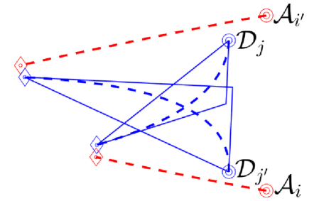
Figure 3: Collision Check via Triangle Intersection

The collisionTime function requires more time to run than triInt. Hence, using triInt as a qualitative check to decide if indeed collision occurs, and then using collisionTime to find the time of collision, reduces on average the total computation time. As shown in Table I, Algorithm 1 on average runs almost four times faster compared to just running collisionTime for all possible pairs of trajectories.

$\downarrow$ Algorithm $\|\;N_{a}\rightarrow$	15	20	25	30
Algorithm 1	61.0	208.3	502.3	1057.1
Only collisionTime	222.1	760.3	1901.4	3883.5

Table I: Computation time (s) to find collision times

The solution to (16) always yields an assignment for which defenders do not collide with each other if (i) all the players play optimally as per (7) and (8), and (ii) such an assignment exists. However, there exist some set of initial states of the players for which such a collision-free assignment does not exist. Furthermore, the attackers may play time-sub-optimally, in which case the defenders may collide with each other under the original assignment, irrespective of whether the original assignment was collision-free or not. In such cases, the time-optimal control action of the involved defenders is augmented by a control term that is based on a control barrier function (CBF). We provide a CBF-based quadratically constrained quadratic program (QCQP) to minimally augment the optimal control of the defenders in the following subsection.

IV-A Control for inter-defender collision avoidance

Let $h_{jj^{\prime}}(t):\mathcal{X}\rightarrow\mathbb{R}$ be defined as $h_{jj^{\prime}}(t)=(\rho_{d}^{col})^{2}-\left\lVert\mathbf{r}_{dj}(t)-\mathbf{r}_{dj^{\prime}}(t)\right\rVert^{2}$. We require that $h_{jj^{\prime}}(t)\leq 0,\;\forall t\geq 0$ for all $j\neq j^{\prime}\in I_{d}$ to ensure that the defenders do not collide with each other. In other words, we want the safe set $\mathcal{X}_{safe}$ to be forward invariant, where $\mathcal{X}_{safe}=\{\mathbf{X}\in\mathcal{X}\;|\;h_{jj^{\prime}}(t)\leq 0,\forall j,j^{\prime}\in I_{d},j\neq j^{\prime}\}$ where the combined state vector $\mathbf{X}=[\mathbf{x}_{d1}^{T},\mathbf{x}_{d2}^{T},...,\mathbf{x}_{dN_{d}}^{T},\mathbf{x}_{a1}^{T},\mathbf{x}_{a2}^{T},...,\mathbf{x}_{aN_{a}}^{T}]^{T}$. A sufficient condition in order to render a set forward invariant is given in terms of a Control Barrier Function (CBF), while Quadratic programs (QPs) subject to CBF constraints have been proposed in recent literature to yield real-time implementable control solutions that can be used to augment nominal controllers at each time step for collision avoidance [27, 21, 28, 22]. In our problem, since the function $h_{jj^{\prime}}(t)$ has relative degree 2 with respect to (w.r.t) the dynamics (1), we resort to the class of exponential CBF (ECBF) [21, 22] for collision avoidance. For the ease of notation, we drop the argument $t$ in the following text. Let $\Delta\mathbf{u}=[\Delta\mathbf{u}_{d1}^{T},\Delta\mathbf{u}_{d2}^{T},...,\Delta\mathbf{u}_{dN_{d}}^{T}]^{T}\in\mathbb{R}^{1\times 2N_{d}}$ be the input correction vector for inter-defender collision avoidance, where $\Delta\mathbf{u}_{dj}$ is the input correction to $\mathcal{D}_{j}$, for all $j\in I_{d}$. Following [21], we define the following relative degree 2 ECBF that is tailored to the application in this paper.

Definition 1

[Exponential Control Barrier Function] Consider a pair of defenders $\mathcal{D}_{j}$ and $\mathcal{D}_{j^{\prime}}$, their dynamics given by (1) and the set $\mathcal{X}_{0}=\{\mathbf{X}_{jj^{\prime}}\in\mathcal{X}_{d}^{2}|\;h_{jj^{\prime}}\leq 0\}$, where $\mathbf{X}_{jj^{\prime}}=[\mathbf{x}_{dj}^{T},\mathbf{x}_{dj^{\prime}}^{T}]^{T}$ and $h_{jj^{\prime}}$ has relative degree 2. $h_{jj^{\prime}}$ is an Exponential Control Barrier Function (ECBF) if there exists $k_{jj^{\prime}}\in\mathbb{R}$ such that,

$$\inf_{\Delta\mathbf{u}_{dj},\Delta\mathbf{u}_{dj^{\prime}}}\ddot{h}_{jj^{\prime}}+2k_{jj^{\prime}}\dot{h}_{jj^{\prime}}+k_{jj^{\prime}}^{2}h_{jj^{\prime}}\leq 0,\forall\mathbf{X}_{jj^{\prime}}\in\mathcal{X}_{0}$$ (17)

and $h_{jj^{\prime}}\leq C_{jj^{\prime}}e^{A_{jj^{\prime}}t}\eta_{jj^{\prime}}\leq 0$ when $\mathbf{X}_{jj^{\prime}}(0)\in\mathcal{X}_{0}$, where $A_{jj^{\prime}}\in\mathbb{R}^{2}$ depends on $k_{jj^{\prime}}$, and $C_{jj^{\prime}}=[1,0]$, $\eta_{jj^{\prime}}=[h_{jj^{\prime}},\dot{h}_{jj^{\prime}}]$.

Next, building on the ECBF-QP formulation in [21, 22], we develop the following ECBF-QCQP as we have quadratic constraint on the control inputs.

$$\displaystyle\min_{\Delta\mathbf{u}} \quad\left\lVert\Delta\mathbf{u}\right\rVert^{2}$$ (18a)

s.t. $$\;1)\;\mathbf{A}_{jj^{\prime}}\Delta\mathbf{u}-b_{jj^{\prime}}\leq 0,\;\forall j^{\prime}\in I_{d},\forall j<j^{\prime};$$ (18b)

$$\;2)\;\left\lVert\mathbf{u}_{dj}^{*}+\Delta\mathbf{u}_{dj}\right\rVert^{2}-(\bar{u}_{d})^{2}\leq 0,\quad\forall j\in I_{d};$$ (18c)

where $\mathbf{A}_{jj^{\prime}}=[0,...,-2(\mathbf{r}_{dj}-\mathbf{r}_{dj^{\prime}})^{T},...,2(\mathbf{r}_{dj}-\mathbf{r}_{dj^{\prime}})^{T},...,0]\in\mathbb{R}^{1\times 2N_{d}}$, $b_{jj^{\prime}}=-2k_{jj^{\prime}}\dot{h}_{jj^{\prime}}-k_{jj^{\prime}}^{2}h_{jj^{\prime}}+2(\left\lVert\mathbf{v}_{dj}-\mathbf{v}_{dj^{\prime}}\right\rVert^{2}+(\mathbf{r}_{dj}-\mathbf{r}_{dj^{\prime}})^{T}(\mathbf{u}_{dj}^{*}-C_{D}\mathbf{v}_{dj}-\mathbf{u}_{dj^{\prime}}^{*}+C_{D}\mathbf{v}_{dj^{\prime}}))$. The constraints in (18b) are the safety constraints as established by ECBF (Definition 1) and those in (18c) are quadratic constraints on the control input. The constant coefficients $k_{jj^{\prime}}>0,\;\forall j\neq j^{\prime}\in I_{d}$, are chosen appropriately to ensure that above QCQP is feasible. Below we explain how to choose appropriate values of $k_{jj^{\prime}}$.

Let us define $\psi_{jj^{\prime}}(t)$ as

$$\psi_{jj^{\prime}}(t)=\dot{h}_{jj^{\prime}}(t)+k_{jj^{\prime}}h_{jj^{\prime}}(t).$$ (19)

To ensure forward invariance of the safe set of the defenders using exponential CBFs [21, 22] the initial states of the defenders need to satisfy Condition 1.

Condition 1

1) $h_{jj^{\prime}}(0)\leq 0$, and 2) $\psi_{jj^{\prime}}(0)\leq 0$, for all $j\neq j^{\prime}\in I_{d}$.

To ensure that $\psi_{jj^{\prime}}(0)\leq 0$ in $S_{jj^{\prime}}(\rho_{0})=\{\mathbf{x}_{dj}(0),\;\mathbf{x}_{dj^{\prime}}(0)\in\mathbb{R}^{2}\times\mathcal{B}_{\bar{v}_{d}}|\left\lVert\mathbf{r}_{dj}(0)-\mathbf{r}_{dj^{\prime}}(0)\right\rVert>\rho_{0}\}$, the coefficient $k_{jj^{\prime}}$ has to satisfy: $\frac{4\bar{v}_{d}\rho_{0}}{\rho_{0}^{2}-(\rho_{d}^{col})^{2}}\leq k_{jj^{\prime}}$. Here $\rho_{0}=2\rho_{d}^{b}+\rho_{d}^{col}$, with $\rho_{d}^{b}=\frac{\bar{u}_{d}(1-\log(2))}{C_{D}^{2}}$ being the breaking distance travelled by a defender moving with the maximum velocity despite maximum acceleration applied opposite to its velocity and $\rho_{d}^{col}>0$ being the safety distance between the defenders. One can choose $k_{jj^{\prime}}(\geq\frac{4\bar{v}_{d}\rho_{0}}{\rho_{0}^{2}-(\rho_{d}^{col})^{2}})$ depending on the initial conditions of the defenders that lie in $S_{jj^{\prime}}(\rho_{0})$ to ensure that the QCQP is always feasible for all future times.

Next, we show that the solution to the ECBF-QCQP in (18) is continuously differentiable (hence locally Lipschitz) almost everywhere in the set $\bar{\mathcal{X}}_{safe}$ defined as

$$\bar{\mathcal{X}}_{safe}=\big{\{}\mathbf{X}\in\mathcal{X}_{safe}|\psi_{jj^{\prime}}(t)\leq 0,\forall j\neq j^{\prime}\in I_{d}\big{\}}.$$ (20)

We first present Lemma 2.

Lemma 2

Let, without loss of generality, that the attackers $\mathcal{A}_{j}$ and $\mathcal{A}_{j^{\prime}}$ are assigned to the defender $\mathcal{D}_{j}$ and $\mathcal{D}_{j^{\prime}}$, respectively, and $\mathcal{X}_{2}=\mathcal{X}_{a}^{2}\times\mathcal{X}_{d}^{2}$ be the configuration space of two defenders and two attackers. Then, the set $Q_{0}=\{[\mathbf{x}_{aj}^{T},\mathbf{x}_{aj^{\prime}}^{T},\mathbf{x}_{dj}^{T},\mathbf{x}_{dj^{\prime}}^{T}]^{T}\in\mathcal{X}_{2}|\;b_{jj^{\prime}}=0,\forall j\neq j^{\prime}\in I_{d}\}$ is a measure zero set.

Proof:

To show that $Q_{0}\subset\mathcal{X}_{2}$ is a measure zero set, we first consider a subset of $\mathcal{X}_{2}$ in which we fix the states $\mathbf{x}_{dj}$, $\mathbf{x}_{aj}$, $\mathbf{x}_{aj^{\prime}}$ and position $\mathbf{r}_{dj^{\prime}}$ of $\mathcal{D}_{j}$, $\mathcal{A}_{j}$, $\mathcal{A}_{j^{\prime}}$ and $\mathcal{D}_{j^{\prime}}$ respectively, and vary the velocity $\mathbf{v}_{dj^{\prime}}$ of $\mathcal{D}_{j^{\prime}}$ such that $\mathbf{v}_{dj^{\prime}}=v[C(\theta),S(\theta)]^{T}$ for fixed value of $v$ and different values of $\theta$ (see Figure 4), i.e., we fix the speed of $\mathcal{D}_{j^{\prime}}$ and vary the direction of its velocity vector.

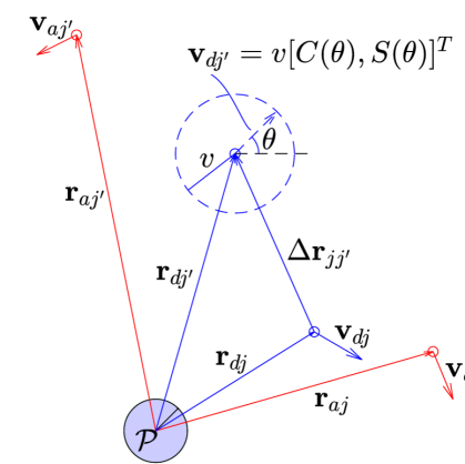
Figure 4: Visualization of the set $\bar{\mathcal{X}}_{2}(\mathbf{x}_{aj},\mathbf{x}_{aj^{\prime}},\mathbf{x}_{dj},\mathbf{r}_{dj^{\prime}},v)$. Solid vectors denote the fixed vectors and the dotted one denotes the variable vector, the dotted circle represents the set $\bar{\mathcal{X}}_{2}(\mathbf{x}_{aj},\mathbf{x}_{aj^{\prime}},\mathbf{x}_{dj},\mathbf{r}_{dj^{\prime}},v)$

We denote this subset of $\mathcal{X}_{2}$ as $\bar{\mathcal{X}}_{2}(\mathbf{x}_{aj},\mathbf{x}_{aj^{\prime}},\mathbf{x}_{dj},\mathbf{r}_{dj^{\prime}},v)=\bar{\mathcal{X}}_{2}=\{\mathbf{v}_{dj^{\prime}}\in\mathcal{B}_{\bar{v}_{d}}|\left\lVert\mathbf{v}_{dj^{\prime}}\right\rVert=v\}$. Now we want to find for what values of $\theta$, we have $b_{jj^{\prime}}=0$ on the set $\bar{\mathcal{X}}_{2}(\mathbf{x}_{aj},\mathbf{x}_{aj^{\prime}},\mathbf{x}_{dj},\mathbf{r}_{dj^{\prime}},v)$. On the set $\bar{\mathcal{X}}_{2}(\mathbf{x}_{aj},\mathbf{x}_{aj^{\prime}},\mathbf{x}_{dj},\mathbf{r}_{dj^{\prime}},v)$, we have:

$$\begin{array}[]{ll}b_{jj^{\prime}}&=-2k_{jj^{\prime}}\dot{h}_{jj^{\prime}}-k_{jj^{\prime}}^{2}h_{jj^{\prime}}+2(\left\lVert\mathbf{v}_{dj}-\mathbf{v}_{dj^{\prime}}\right\rVert^{2}+\\ &\quad(\Delta\mathbf{r}_{jj^{\prime}})^{T}(\mathbf{u}_{dj}^{*}-C_{D}\mathbf{v}_{dj}-\mathbf{u}_{dj^{\prime}}^{*}+C_{D}\mathbf{v}_{dj^{\prime}}))\\ &=\underbrace{-k_{jj^{\prime}}^{2}h_{jj^{\prime}}+2(\Delta\mathbf{r}_{jj^{\prime}}^{T}(\mathbf{u}_{dj}^{*}-C_{k_{jj^{\prime}}}\mathbf{v}_{dj})\left\lVert\mathbf{v}_{dj}\right\rVert^{2}+v^{2})}_{T_{1}}\\ &\quad\underbrace{-2\big{(}\Delta\mathbf{r}_{jj^{\prime}}^{T}(\bar{u}_{d}^{\prime}\hat{\mathbf{o}}(\theta_{dj^{\prime}}^{*})-C_{k_{jj^{\prime}}}v\hat{\mathbf{o}}(\theta))+v\mathbf{v}_{dj^{\prime}}^{T}\hat{\mathbf{o}}(\theta)\big{)}}_{T_{2}}\end{array}$$ (21)

where $\Delta\mathbf{r}_{jj^{\prime}}=\mathbf{r}_{dj}-\mathbf{r}_{dj^{\prime}}$, $\hat{\mathbf{o}}(\theta)=[C(\theta),S(\theta)]^{T}$, $C_{k_{jj^{\prime}}}=C_{D}-k_{jj^{\prime}}$ and $\theta_{dj^{\prime}}^{*}$ is dependent on $\theta$. On $\bar{\mathcal{X}}_{2}(\mathbf{x}_{aj},\mathbf{x}_{aj^{\prime}},\mathbf{x}_{dj},\mathbf{r}_{dj^{\prime}},v)$ the term $T_{2}$ in (21) depends on $\theta$ while $T_{1}$ does not. The term $T_{2}$ can be further simplified as:

$$\begin{array}[]{ll}T_{2}&=-2\big{(}\Delta\mathbf{r}_{jj^{\prime}}^{T}(\bar{u}_{d}^{\prime}\hat{\mathbf{o}}(\theta_{dj^{\prime}}^{*})-C_{k_{jj^{\prime}}}v\hat{\mathbf{o}}(\theta))+v\mathbf{v}_{dj^{\prime}}^{T}\hat{\mathbf{o}}(\theta)\big{)}\\ &=-2\big{(}\left\lVert\Delta\mathbf{r}_{jj^{\prime}}\right\rVert(\bar{u}_{d}^{\prime}\cos(\theta_{ru}+\theta_{dj^{\prime}}^{*})-C_{k_{jj^{\prime}}}v\cos(\theta_{rv}+\theta))\\ &\quad+v\left\lVert\mathbf{v}_{dj^{\prime}}\right\rVert\cos(\theta_{vv}+\theta)\big{)}\end{array}$$ (22)

where $\theta_{ru}$, $\theta_{rv}$, $\theta_{vv}$ are the angles between vectors $\Delta\mathbf{r}_{jj^{\prime}}$ and $\mathbf{u}_{dj^{\prime}}^{*}$, $\Delta\mathbf{r}_{jj^{\prime}}$ and $\mathbf{v}_{dj^{\prime}}$, and vectors $\mathbf{v}_{dj}$ and $\mathbf{v}_{dj^{\prime}}$, respectively, when $\theta=0$. From (22) we observe that $T_{2}$ is a sum of weighted cosines that depend on $\theta$. This means $T_{2}$ can be 0 only for a countably finite number of values of $\theta$ in the set $[0,2\pi]$. This implies that $b_{jj^{\prime}}$ can be 0 on $\bar{\mathcal{X}}_{2}(\mathbf{x}_{aj},\mathbf{x}_{aj^{\prime}},\mathbf{x}_{dj},\mathbf{r}_{dj^{\prime}},v)$ only for a countably finite number of values of $\theta$. Let this set of values of $\theta$ be denoted as $\bar{Q}_{0}$. Then we have that the set $\bar{Q}_{0}\subset\bar{\mathcal{X}}_{2}(\mathbf{x}_{aj},\mathbf{x}_{aj^{\prime}},\mathbf{x}_{dj},\mathbf{r}_{dj^{\prime}},v)$ is a measure zero subset of $\bar{\mathcal{X}}_{2}(\mathbf{x}_{aj},\mathbf{x}_{aj^{\prime}},\mathbf{x}_{dj},\mathbf{r}_{dj^{\prime}},v)$. Next, we have that the configuration space $\mathcal{X}_{2}$ of $\mathcal{D}_{j}$, $\mathcal{D}_{j^{\prime}}$, $\mathcal{A}_{j}$, $\mathcal{A}_{j^{\prime}}$ is a union of all possible disjoint sets $\bar{\mathcal{X}}_{2}(\mathbf{x}_{aj},\mathbf{x}_{aj^{\prime}},\mathbf{x}_{dj},\mathbf{r}_{dj^{\prime}},v)$. This implies that the set $Q_{0}$ is exactly the union of all possible subsets $\bar{Q}_{0}$, i.e., $Q_{0}=\cup\bar{Q}_{0}$. Since each $\bar{Q}_{0}$ is a measure zero subset, we have that the set $Q_{0}$ is also a measure zero set [29]. ∎

Next, we make the following assumption.

Assumption 3

The total number of active constraints in (18) at the nominal control $\mathbf{u}_{dj}^{*}$ (i.e., at $\Delta\mathbf{u}_{dj}=\mathbf{0}$) for all $j\in I_{d}$, at any time is less then $2N_{d}$.

Assumption 3 ensures that the gradients of the active constraints at the nominal control $\mathbf{u}_{dj}^{*}$, for all $j\in I_{d}$, are linearly independent. The constraints in (18c) can never be active at the nominal control because $\left\lVert\mathbf{u}_{dj}^{*}\right\rVert=\bar{u}_{d}^{\prime}=\bar{u}_{d}-\epsilon_{d}$. Hence the Assumption 3 practically implies that only any $N_{d}$ pairs of the defenders have their corresponding safety constraint in (18b) active under the nominal control (i.e., at $\Delta\mathbf{u}_{dj}=\mathbf{0}$). In other words, Assumption 3 enforces that maximum $N_{d}$ pairs of defenders could possibly be on a collision course.

Next, in Theorem 3 we prove that the solution to the ECBF-QCQP (18) is continuously differentiable almost everywhere.

Theorem 3

Under Assumption 3, i) the solution to the ECBF-QCQP in (18) is continuously differentiable (and hence locally Lipschitz) on $\bar{\mathcal{X}}_{safe}\backslash Q_{0}$.

Proof:

We observe that: 1) the objective function and the constraints defining the QCQP (18) are twice continuously differentiable functions of $\Delta\mathbf{u}$ and $\mathbf{U}=(\mathbf{x}_{d1},\mathbf{x}_{d2},...,\mathbf{x}_{dN_{d}},\mathbf{u}_{d1}^{*},\mathbf{u}_{d2}^{*},...,\mathbf{u}_{dN_{d}}^{*})$, 2) the gradients of the active constraints with respect to $\Delta\mathbf{u}$ are linearly independent under Assumption 3, 3) the Hessian of the Lagrangian, $H=\mathbf{I}_{2N_{d}}+\sum_{l=1}^{N_{c}}\mu_{l}\mathbf{I}_{2N_{d}}$, is positive definite, where $\mathbf{I}_{2N_{d}}$ is the identity matrix in $\mathbb{R}^{2N_{d}\times 2N_{d}}$ and $\mu_{l}\geq 0$ are Lagrangian multipliers. Furthermore, since we use $\bar{u}_{d}^{\prime}=\bar{u}_{d}-\epsilon_{d}$ to obtain the nominal time-optimal control $\mathbf{u}_{dj}^{*}$, the constraints in (18c) will never be active at the nominal control $\mathbf{u}_{dj}^{*}$ (i.e., at $\Delta\mathbf{u}=\bm{0}$). This implies that the strict complementary slackness condition holds for (18) almost everywhere except for a set $Q_{0}=\{[\mathbf{x}_{aj}^{T},\mathbf{x}_{aj^{\prime}}^{T},\mathbf{x}_{dj}^{T},\mathbf{x}_{dj^{\prime}}^{T}]^{T}\in\mathcal{X}_{2}|;b_{jj^{\prime}}=0,\forall j\neq j^{\prime}\in I_{d}\}$. From Lemma 2 we have that $Q_{0}$ is a measure zero set. Then, using the Theorem 2.1 in [30], the solution to (18) is shown to be a continuously differentiable function of $\mathbf{U}$ in $\bar{\mathcal{X}}_{safe}\backslash Q_{0}$ and hence the solution is also locally Lipschitz continuous in $\bar{\mathcal{X}}_{safe}\backslash Q_{0}$.

∎

Proving forward invariance of the set $\bar{\mathcal{X}}_{safe}$ using tools such as Nagumo’s Theorem [31] that is commonly used in CBF community requires existence and uniqueness of the system trajectories for all future times. However, with the Theorem 3 we are only able to establish local Lipschitz continuity of the solution to ECBF-QCQP (18) on the set $\bar{\mathcal{X}}_{safe}\backslash Q_{0}$, and hence uniqueness of the defenders’ trajectories on $\bar{\mathcal{X}}_{safe}\backslash Q_{0}$ only up-to a maximal time interval $[0,t_{max})$, where $t_{max}>0$ depends on the initial state $\mathbf{X}(0)$ of the players. Note that on the set $Q_{0}$ the strict complimentary slackness may not hold, and hence commenting on the Lipschitz continuity of the solution to the ECBF-QCQP using the existence tools [30, 32] is challenging. The set $Q_{0}$ is also the set in which there is possibility that two defenders will be in a deadlock, i.e., a set from where the defenders are no longer moving. The conditions that lead to deadlocks are dictated by the motion of the attackers and the corresponding nominal optimal interception control (9) of the defenders. However, since the attackers’ control strategy is not known a priory, commenting on whether/when these type of behaviours may occur is very challenging, and goes beyond the scope of the current paper, which is to introduce a collision-aware defender-to-attacker assignment protocol. The CBF-based collision avoidance control is provided for complementing the collision-aware interception strategy, and because it allows us to minimally augment the nominal optimal interception control only when needed. However, as mentioned earlier, the safety analysis of the multi-agent system using CBF-based collision avoidance control is very challenging, and hence it will be investigated in our future work as an independent study.

V Simulation Results

In this section, we provide MATLAB simulations for various scenarios to demonstrate the effectiveness of inter-defender collision-aware interception strategy (IDCAIS), the overall defense strategy that combines CADAA and ECBF-QCQP. Some key parameters used in the simulations are: $\rho_{a}=\rho_{d}=0.5\hskip 1.42262ptm$, $C_{D}=0.5$, $\bar{v}_{a}=6\hskip 1.42262ptms^{-1}\;(\bar{u}_{a}=3\hskip 1.42262ptms^{-2})$, $\bar{v}_{d}=6.8\hskip 1.42262ptms^{-1}\;(\bar{u}_{d}=3.4\hskip 1.42262ptms^{-2})$, $\rho_{d}^{int}=1\hskip 1.42262ptm$, $\rho_{d}^{col}=2\hskip 1.42262ptm$, $\mathbf{r}_{p}=[0,0]^{T}$, $\rho_{p}=2\hskip 1.42262ptm$ and $w=0.5$ .

V-1 Attackers use time-optimal control

Consider Scenario 1 with two defenders (in blue) and two attackers (in red) as shown in Figure 5(a) both operating under their time-optimal control actions with no active collision-avoidance control on the defenders. The optimal paths of the players are shown in solid when CADAA is used to assign defenders to the attackers, while for the same initial conditions the dotted paths correspond to the collision-unaware defender-to-attacker assignment (CUDAA). Here CUDAA is obtained based only on the linear term in the objective in (16), which attempts to minimize the sum of the times of interception expected to be taken by the defenders. CUDAA results into $\mathcal{D}_{1}\rightarrow\mathcal{A}_{1}$ and $\mathcal{D}_{2}\rightarrow\mathcal{A}_{2}$ assignment, while CADAA results into $\mathcal{D}_{1}\rightarrow\mathcal{A}_{2}$ and $\mathcal{D}_{2}\rightarrow\mathcal{A}_{1}$ assignment. In Figure 6(a), the distance between the defenders is shown for CADAA (solid) and CUDAA (dashed). The dotted pink line in Figure 6(a) and subsequent figures denote the minimum safety distance $\rho_{d}^{col}$ between the defenders. Note that the defenders collide with each other under CUDAA, which does not account for the possible future collisions among the defenders. On the other hand, CADAA helps avoid the impending collision between the defenders at the cost of delayed interception of the attackers.

In Figure 5(b), Scenario 2 is shown where the CADAA is unable to prevent the collision between the defenders. This is evident from the plot of the distance between the defenders in both cases (Figure 6(b)). The CADAA only helps in delaying the collision between the defenders.

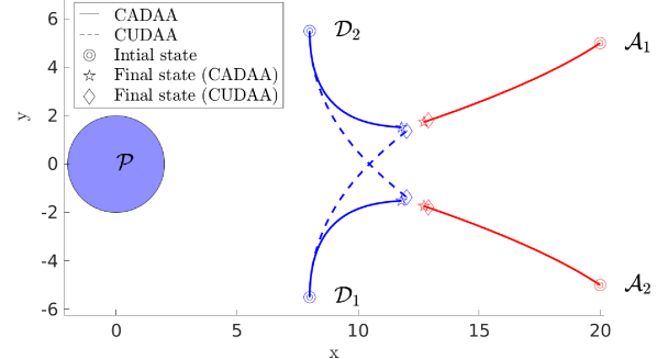
(a) Scenario 1: CADAA helps avoid inter-defender collision

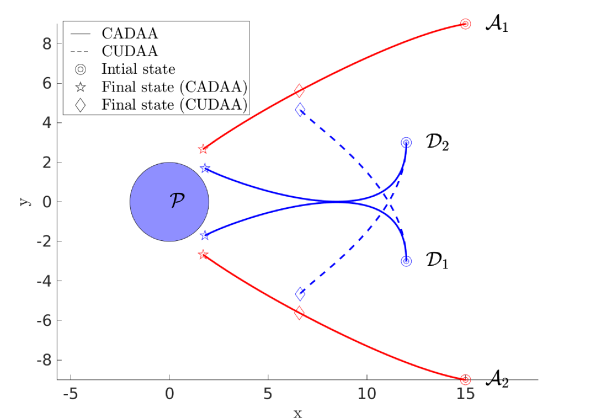
(b) Scenario 2: CADAA only delays inter-defender collision

Figure 5: Trajectories of the players under CADAA and CUDAA (blue: defenders, red: attackers)

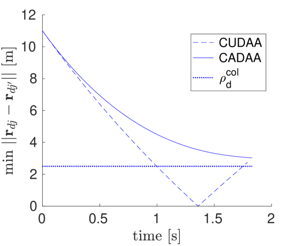
(a) Minimum distance between the defenders for the trajectories in Scenario 1

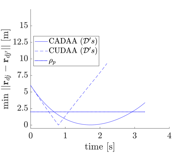
(b) Minimum distance between the defenders for the trajectories in Scenario 2

Figure 6: Minimum distance between defenders under CADAA and CUDAA (blue: defenders, red: attackers)

Since it is impossible to avoid collisions in some cases even after accounting for future collisions during the assignment stage, in Figure 7, we show how the ECBF-QCQP based correction helps defenders avoid collisions with each other. In Figure 7(a) Scenario 3 is shown where despite CADAA the defenders would collide (dashed paths), but after the ECBF-QCQP corrections the defenders avoid collisions (solid paths in Figure7(a), see also distances in Figure 8(a)) and are also able to intercept the attackers before the attackers reach the protected area. Due to active collision avoidance among the defenders, the interception of the attackers is delayed compared to the case when there is no active collision avoidance used by the defenders. This may result into scenarios where the defenders engage in collision avoidance but fail to intercept the attackers. An example of such scenarios is shown in 7(b), Scenario 4, where the defenders avoid collision with each other (see Figure 8(b) for distances) but they are unable to intercept both the attackers in time, attacker $\mathcal{A}_{1}$ is able to reach the protected area before the defender $\mathcal{D}_{2}$ could intercept it (see Figure 8(b)).

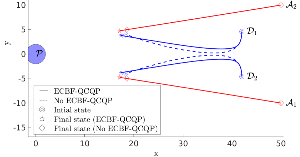
(a) Scenario 3: Defenders avoid collision with each other and also capture the attackers

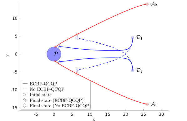
(b) Scenario 4: Defenders avoid collision with each other but fail to capture the attackers

Figure 7: Trajectories of the players under CADAA with collision avoidance control (ECBF-QCQP), i.e., IDCAIS, and without collision avoidance control (no ECBF-QCQP) (blue: defenders, red: attackers)

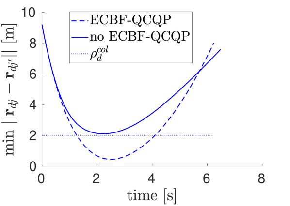
(a) Minimum distance between the defenders for the trajectories in Scenario 3)

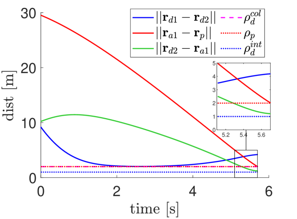
(b) Minimum distance between the defenders for the trajectories in Scenario 4

Figure 8: Minimum distance between the defenders under IDCAIS (CADAA & ECBF-QCQP) (blue: defenders, red: attackers)

V-2 Attackers use time-sub-optimal control

Sometimes the attackers may not use time-optimal control, for instance in an attempt to escape from the defenders. In Figure 9(a), Scenario 5 is shown where a time-sub-optimal behavior hampers their chances of hitting the protected area. The dotted curves correspond to the time-optimal behavior by the attackers. As observed, the attacker $\mathcal{A}_{3}$ could have succeeded in reaching the protected area had it played optimally. However, $\mathcal{A}_{3}$’s attempt to escape from $\mathcal{D}_{3}$ gives more time to $\mathcal{D}_{3}$ to capture $\mathcal{A}_{3}$, and $\mathcal{D}_{3}$ indeed captures $\mathcal{A}_{3}$ (see the solid curves in Figure 9(a)) while all defenders stay safe with respect to each other (Figure 10(a)).

In an another scenario shown in Figure 9(b), Scenario 6, again due to the active inter-defender collision avoidance (Figure 10(b)) the defender $\mathcal{D}_{3}$ fails to intercept $\mathcal{A}_{3}$ despite the fact that: 1) $\mathcal{A}_{3}$ uses time-sub-optimal control in an attempt to escape from the defenders, and 2) had $\mathcal{A}_{3}$ played time-optimally, it would have been captured by $\mathcal{D}_{3}$. This shows that while having active inter-defender collision is beneficial for the safety of the defenders, it also compromises the interception performance.

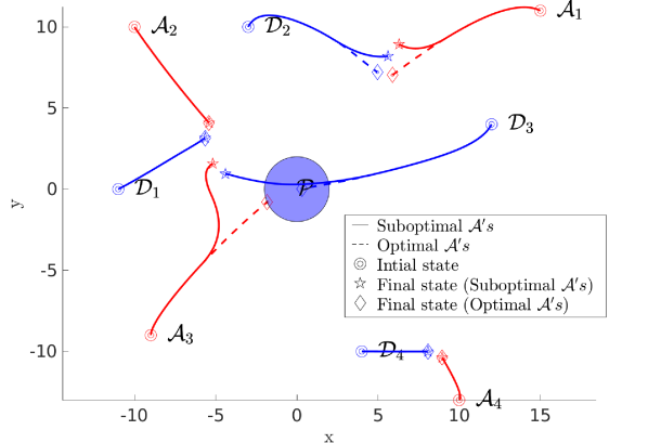
(a) Scenario 5: Defenders capture time-sub-optimal attackers

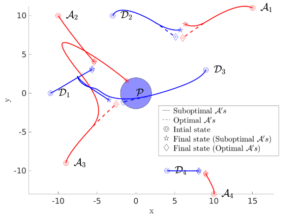
(b) Scenario 6: Defenders fail to capture the time-sub-optimal attackers due to active inter-defender collision avoidance

Figure 9: Trajectories of the players under IDCAIS against time-sub-optimal behavior by the attackers (blue: defenders, red: attackers)

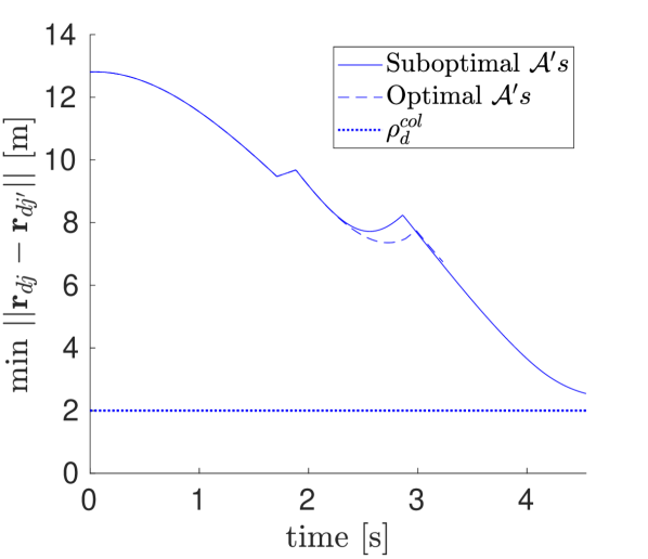
(a) Minimum distance between the defenders for the trajectories in Scenario 5

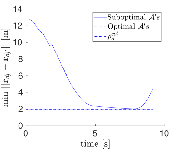
(b) Minimum distance between the defenders for the trajectories in Scenario 6

Figure 10: Minimum distance between the defenders under IDCAIS against time-sub-optimal behavior by the attackers (blue: defenders, red: attackers)

A video of the above discussed simulations can be found at https://tinyurl.com/4mhdpye9.

V-3 Effectiveness of CADAA

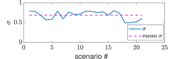
Figure 11: Success rate of CADAA

We provide a numerical evaluation of the effectiveness of the proposed collision-aware interception strategy. It is numerically intractable to evaluate all possible scenarios even for 2 defenders vs 2 attackers. So, we discretize the state space, fix the initial states of the 2 attackers and 1 defender, and vary the state of the other defender. We then evaluate CADAA success rate, $\sigma=\frac{\text{ \# cases for which CADAA is able to avoid the collisions}}{\text{\# cases for which CUDAA results into defenders' collision}}$. We do this for 20 scenarios of fixed states of the attackers and the defender and plot the values of $\sigma$ in Figure 11. As observed in Figure 11, on average in 68% cases CADAA helps avoid the collision between the defenders.

VI Conclusions and Future Work

In this paper, we proposed inter-defender collision-aware interception strategy for a team of defenders moving under damped double integrator models to intercept multiple attackers. We used time-optimal, collision-aware, defender-to-attacker assignment (CADAA) to optimally assign defenders to attackers, and exponential-CBF-based QCQP for active inter-defender collision avoidance. The effectiveness and limitations of the proposed strategy are demonstrated formally as well as through simulations for attackers’ time-optimal and as time-sub-optimal behaviors.

The proposed collision-aware assignment (CADAA) requires solving a Mixed-Integer Quadratic Program (MIQP), which is computationally challenging as the number of the involved players increases. As a future work, we plan to investigate computationally-efficient heuristics in order to solve the MIQP presented in this paper, and therefore reduce the computation time of CADAA.

Another interesting future direction for this work could be an extension to scenarios with multiple protected areas under attack from the attackers. In such scenario, the defenders can (i) infer which protected area a given attacker is going to, (ii) design the best-against-worst time optimal control described in Section III corresponding to the identified protected area, and (iii) make collision-aware assignments of the defenders using CADAA that uses the costs obtained for the defender-attacker pair corresponding the identified protected area/areas.

References

- [1] R. Isaacs, Differential games: a mathematical theory with applications to warfare and pursuit, control and optimization. Courier Corporation, 1999.
- [2] R. H. Venkatesan and N. K. Sinha, “The target guarding problem revisited: Some interesting revelations,” IFAC Proceedings Volumes, vol. 47, no. 3, pp. 1556–1561, 2014.
- [3] M. Pachter, E. Garcia, and D. W. Casbeer, “Differential game of guarding a target,” Journal of Guidance, Control, and Dynamics, vol. 40, no. 11, pp. 2991–2998, 2017.
- [4] M. W. Harris, “Abnormal and singular solutions in the target guarding problem with dynamics,” Journal of Optimization Theory and Applications, vol. 184, no. 2, pp. 627–643, 2020.
- [5] J. Mohanan, N. Kothuri, and B. Bhikkaji, “The target guarding problem: A real time solution for noise corrupted measurements,” European Journal of Control, vol. 54, pp. 111–118, 2020.
- [6] H. Huang, J. Ding, W. Zhang, and C. J. Tomlin, “A differential game approach to planning in adversarial scenarios: A case study on capture-the-flag,” in 2011 IEEE International Conference on Robotics and Automation. IEEE, 2011, pp. 1451–1456.
- [7] A. Pierson, Z. Wang, and M. Schwager, “Intercepting rogue robots: An algorithm for capturing multiple evaders with multiple pursuers,” IEEE Robotics and Automation Letters, vol. 2, no. 2, pp. 530–537, 2016.
- [8] M. Chen, Z. Zhou, and C. J. Tomlin, “Multiplayer reach-avoid games via pairwise outcomes,” IEEE Transactions on Automatic Control, vol. 62, no. 3, pp. 1451–1457, 2017.
- [9] D. Shishika, J. Paulos, and V. Kumar, “Cooperative team strategies for multi-player perimeter-defense games,” IEEE Robotics and Automation Letters, vol. 5, no. 2, pp. 2738–2745, 2020.
- [10] M. Coon and D. Panagou, “Control strategies for multiplayer target-attacker-defender differential games with double integrator dynamics,” in Decision and Control (CDC), 2017 IEEE 56th Annual Conference on. IEEE, 2017, pp. 1496–1502.
- [11] Y. Zheng, X. Shao, Z. Chen, and W. Zhao, “Time-optimal guidance to intercept moving targets by dubins vehicles,” arXiv preprint arXiv:2012.11855, 2020.
- [12] E. Garcia, D. W. Casbeer, and M. Pachter, “Optimal target capture strategies in the target-attacker-defender differential game,” in 2018 Annual American Control Conference (ACC). IEEE, 2018, pp. 68–73.
- [13] M. Pachter, D. W. Casbeer, and E. Garcia, “Capture-the-flag: A differential game,” in 2020 IEEE Conference on Control Technology and Applications (CCTA). IEEE, 2020, pp. 606–610.
- [14] B. Landry, M. Chen, S. Hemley, and M. Pavone, “Reach-avoid problems via sum-or-squares optimization and dynamic programming,” in 2018 IEEE/RSJ International Conference on Intelligent Robots and Systems (IROS). IEEE, 2018, pp. 4325–4332.
- [15] J. Lorenzetti, M. Chen, B. Landry, and M. Pavone, “Reach-avoid games via mixed-integer second-order cone programming,” in 2018 IEEE conference on decision and control (CDC). IEEE, 2018, pp. 4409–4416.
- [16] S. Lee, G. E. Dullerud, and E. Polak, “On the real-time receding horizon control in harbor defense,” in 2015 American Control Conference (ACC). IEEE, 2015, pp. 3601–3606.
- [17] S. Lee, E. Polak, and J. Walrand, “A receding horizon control law for harbor defense,” in 2013 51st Annual Allerton Conference on Communication, Control, and Computing (Allerton). IEEE, 2013, pp. 70–77.
- [18] S. H. Lee, “A model predictive control approach to a class of multiplayer minmax differential games,” Ph.D. dissertation, University of Illinois at Urbana-Champaign, 2016.
- [19] R. Yan, X. Duan, Z. Shi, Y. Zhong, and F. Bullo, “Matching-based capture strategies for 3d heterogeneous multiplayer reach-avoid differential games,” Automatica, vol. 140, p. 110207, 2022.
- [20] E. Bakolas, “Optimal guidance of the isotropic rocket in the presence of wind,” Journal of Optimization Theory and Applications, vol. 162, no. 3, pp. 954–974, 2014.
- [21] Q. Nguyen and K. Sreenath, “Exponential control barrier functions for enforcing high relative-degree safety-critical constraints,” in 2016 American Control Conference (ACC). IEEE, 2016, pp. 322–328.
- [22] L. Wang, A. D. Ames, and M. Egerstedt, “Safe certificate-based maneuvers for teams of quadrotors using differential flatness,” in 2017 IEEE International Conference on Robotics and Automation (ICRA). IEEE, 2017, pp. 3293–3298.
- [23] D. E. Kirk, Optimal control theory: an introduction. Courier Corporation, 2004.
- [24] D. Feng and B. Krogh, “Acceleration-constrained time-optimal control in n dimensions,” IEEE transactions on automatic control, vol. 31, no. 10, pp. 955–958, 1986.
- [25] F. Blanchini, “Set invariance in control,” Automatica, vol. 35, no. 11, pp. 1747–1767, 1999.
- [26] L. Gurobi Optimization, “Gurobi optimizer reference manual,” 2018. [Online]. Available: http://www.gurobi.com
- [27] A. D. Ames, X. Xu, J. W. Grizzle, and P. Tabuada, “Control barrier function based quadratic programs for safety critical systems,” IEEE Transactions on Automatic Control, vol. 62, no. 8, pp. 3861–3876, 2016.
- [28] W. Xiao and C. Belta, “Control barrier functions for systems with high relative degree,” in 2019 IEEE 58th Conference on Decision and Control (CDC). IEEE, 2019, pp. 474–479.
- [29] V. I. Bogachev and M. A. S. Ruas, Measure theory. Springer, 2007, vol. 1.
- [30] A. V. Fiacco, “Sensitivity analysis for nonlinear programming using penalty methods,” Mathematical programming, vol. 10, no. 1, pp. 287–311, 1976.
- [31] F. Blanchini and S. Miani, Set-theoretic methods in control. Springer, 2008, vol. 78.
- [32] N. N. Tam, “On continuity properties of the solution map in quadratic programming,” Acta Mathematica Vietnamica, vol. 24, pp. 47–61, 1999.