Observation of quantum phase-synchronization in a nuclear spin-system

Abstract

We report an experimental study of phase-synchronization in a pair of interacting nuclear spins subjected to an external drive in nuclear magnetic resonance architecture. A weak transition-selective radio-frequency field applied on one of the spins is observed to cause phase-localization, which is experimentally established by measuring the Husimi distribution function under various drive conditions. To this end, we have developed a general interferometric technique to directly extract values of the Husimi function via the transverse magnetization of the undriven nuclear spin. We further verify the robustness of synchronization to detuning in the system by studying the Arnold tongue behaviour.

I Introduction

Motivated by the stability and ubiquity of classical synchronization [1], quantum synchronization has been a field of intense study. Platforms that exhibit quantized dynamics have inspired theoretical studies in systems such as trapped ions [2, 3], superconducting circuits [4], atomic ensembles [5], optomechanical systems [6, 7, 8, 9] and nanomechanical systems [10, 11]. Theoretical studies have shown fundamental implications of synchronization to other fields such as entanglement generation [12, 13], thermodynamics [14, 15], quantum networks [16] and continuous time crystals[17].

Quantum synchronization proceeds by first considering the quantum analogue of phase space, which is one of many quasiprobability distrubitions such as Husimi function and Wigner function [18]. A valid limit cycle requires robustness against external perturbations and a neutral free phase [1]. Thermal states were shown to be examples of such limit cycle states, showing equiprobable distribution of phases in phase space [14]. Such phase space distribution functions have been used to construct measures of synchronization [7, 19, 20, 21, 22]. Following several studies of synchronization in specific systems, unified measures of quantum synchronization based on relative entropies have also been formulated [23]. They used information theoretic measures based on quantum correlations, which have been shown to measure synchronization [24, 25, 13]. These measures reduce to the phase space based measures under the system specific conditions [23].

Following this theoretical interest [7, 8, 26, 13, 27, 23, 14, 15, 28], quantum synchronization has been experimentally demonstrated recently in the IBM quantum computer [29] and spin-1 cold atoms [30]. The experimental demonstration of quantum synchronization is in general a challenging task owing to the difficulty in extracting required parameters. Quantum synchronization measurements typically require the system to settle into a steady state, which necessitates the need for long waiting times. Such long wait times allow for other experimental noise sources to interfere with the signal. Besides this, tomographic reconstruction of the state scales with the system size, requiring $O(n^{2})$ measurements for a system of dimension $n$ [31]. Thus, the steady state characteristics of the system are inferred by extrapolating transient dynamics or by devising complicated measurement schemes.

Here, we resolve the aforementioned issues and report the observation of synchronization in nuclear spins. Nuclear magnetic resonance (NMR) architecture allows convenient control and manipulation of multi-spin systems using radio frequency (RF) pulses. These, in addition to inherent relaxation mechanisms, which cause the system to thermalize offer an ideal platform to observe synchronization. Our experiment involves a pair of interacting spin-1/2 nuclei and a weak transition-selective RF field applied on one of the spins. The resulting phase-localization is characterized using Husimi distribution, which typically needs quantum state tomography (QST) [32]. However, QST after a long external drive proved to be highly inefficient because, as the steady state is approached, the irradiated levels saturate and relevant transitions become too faint. We overcome this by introducing a new interferometric technique that can experimentally capture the Husimi Q-function directly. In addition, this method can be adapted beyond synchronization to other studies that rely on coherence measurements, even weak ones. By measuring the NMR system in the process of reaching the steady state, we investigate transient as well as steady state behaviour of the system under the influence of the external drive. We also explore the robustness of synchronization against detuning frequency and drive strength via the Arnold tongue.

This article is organized as follows: in Sec. II, we introduce the spin-system and outline the theory as well as measures of quantum synchronization. In Sec. III, we explain the NMR architecture, the experimental setup, and the numerical model. The interferometric measurement of Husimi distribution (IMHD) is described in Sec. IV. Following this, we discuss the corresponding experimental results in Sec. V. Finally, we conclude in Sec. VI.

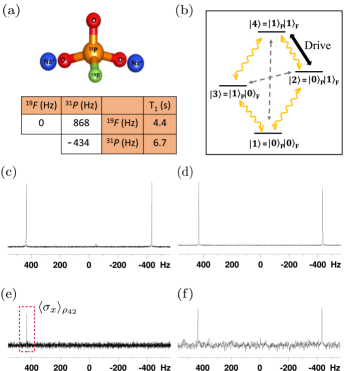
Figure 1: (a) Sodium fluorophosphate molecular structure with its Hamiltonian parameters and the spin-lattice relaxation time constants (T₁) shown in the table. The diagonal elements represent the offset, while off-diagonal element represents the scalar $J$ coupling constant. Figure (b) represents the energy levels of the two-qubit system with four non-degenerate energy eigenstates. The numerical model presented here considers only the single-quantum relaxation pathways (yellow curved arrows) and ignores the zero- and double-quantum pathways (dashed grey arrows). Figures (c,d) show reference NMR spectra of ³¹P and ¹⁹F spins respectively, each obtained with a $90^{\circ}$ pulse on thermal equilibrium state, while (e) shows the ³¹P NMR signal after 100 s drive on the $|{2}\rangle\leftrightarrow|{4}\rangle$ transition. Intensity of the $\rho_{42}$ element is indicated in the dashed box, which is used for the Arnold tongue analysis. Figure (f) shows the ¹⁹F NMR spectrum at the end of interferometric circuit from which we can directly extract the Husimi distribution at a particular $\theta$ and $\phi$ values.

II Synchronization of a four-level system

We consider a non-degenerate four-level system composed of ¹⁹F and ³¹P nuclei in sodium fluorophospate molecule, as shown in Fig. 1(a,b) and study the phase synchronization of the system with an external drive. The extent of phase localization of the system in a state $\rho$ can be quantified using the Husimi-Kano Q representation function [33, 34]. For the given four-level system it can be defined as

$$Q(\theta_{1},\theta_{2},\theta_{3},\phi_{1},\phi_{2},\phi_{3})=\frac{24}{\pi^{3}}\langle{\hat{n}_{4}}|{\rho}|{\hat{n}_{4}}\rangle,$$ (1)

where

$$|{\hat{n}_{4}}\rangle=(C_{\theta_{1}},e^{i\phi_{1}}S_{\theta_{1}}C_{\theta_{2}},e^{i\phi_{2}}S_{\theta_{1}}S_{\theta_{2}}C_{\theta_{3}},e^{i\phi_{3}}S_{\theta_{1}}S_{\theta_{2}}S_{\theta_{3}})^{T},$$

is $SU(4)$ coherent state [35, 36, 37] with $C_{\theta_{i}}=\cos(\theta_{i}/2)$ and $S_{\theta_{i}}=\sin(\theta_{i}/2)$. A brief review of spin coherent states is presented in Appendix A. The normalization of the Q-function arises from the completeness relation of coherent state $|{\hat{n}_{4}}\rangle$ defined as

$$\int|{\hat{n}_{4}}\rangle\langle{\hat{n}_{4}}|d\mu=\frac{\pi^{3}}{24}\mathbbm{1},$$ (2)

where the integration is taken over the Haar measure and volume element given by [36]

$$d\mu=d\theta_{1}d\theta_{2}d\theta_{3}d\phi_{1}d\phi_{2}d\phi_{3}C_{2\theta_{1}}S^{5}_{2\theta_{1}}C_{2\theta_{2}}S_{2\theta_{2}}^{3}C_{2\theta_{3}}S_{2\theta_{3}}.$$

For a system with internal Hamiltonian $H_{0}=\sum_{i=1}^{4}\omega_{i}|{i}\rangle\langle{i}|$ having characteristic frequencies $\omega_{i}$, the spin coherent state evolves as

$$e^{-iH_{0}t}|{\hat{n}_{4}}\rangle\rightarrow\left(\begin{array}[]{c}C_{\theta_{1}}\\ e^{i(\phi_{1}-\omega_{21}t)}S_{\theta_{1}}C_{\theta_{2}}\\ e^{i(\phi_{2}-\omega_{31}t)}S_{\theta_{1}}S_{\theta_{2}}C_{\theta_{3}}\\ e^{i(\phi_{3}-\omega_{41}t)}S_{\theta_{1}}S_{\theta_{2}}S_{\theta_{3}}\end{array}\right),$$ (7)

where $\omega_{i1}=\omega_{i}-\omega_{1}$. Under the free evolution of internal Hamiltonian, $\phi_{i}$s represent the free phases oscillating with the respective frequencies $\omega_{i1}$ while $\theta_{i}$s govern the populations of the system which remains fixed. In the absence of any external perturbation, the steady state reached by the thermalization has uniform phase distribution, and the Husimi Q-function remains independent of $(\phi_{1},\phi_{2},\phi_{3})$. This points to the fact that the given system has free phases available. Along with the existence of free phases, a system needs to be nonlinear in nature to exhibit limit cycle behaviour. Since the dynamics of a multilevel quantum system is generally nonlinear, the availability of free phases makes it a perfect candidate to study synchronization. On application of a weak external drive the system may develop a definite phase relationship with the drive, thus resulting in a localized phase distribution. This phenomenon, known as phase synchronization, is captured and quantified by

$$S(\phi_{1},\phi_{2},\phi_{3}) =\int d\Theta~{}Q(\theta_{1},\theta_{2},\theta_{3},\phi_{1},\phi_{2},\phi_{3})-\frac{1}{(2\pi)^{3}},$$ (8)

where $d\Theta=d\theta_{1}d\theta_{2}d\theta_{3}C_{2\theta_{1}}S^{5}_{2\theta_{1}}C_{2\theta_{2}}S_{2\theta_{2}}^{3}C_{2\theta_{3}}S_{2\theta_{3}}$. For the four-level system considered here, the above expression leads to

$$S(\phi_{1},\phi_{2},\phi_{3}) =\frac{1}{16\pi^{2}}\mathrm{Re}\left[\rho_{43}e^{i\phi_{1}}+\rho_{42}e^{i\phi_{2}}+\rho_{41}e^{i\phi_{3}}\right.$$

$$\left.+\rho_{32}e^{i(\phi_{2}-\phi_{1})}+\rho_{31}e^{i(\phi_{3}-\phi_{1})}+\rho_{21}e^{i(\phi_{3}-\phi_{2})}\right],$$ (9)

where $\rho_{ij}=\langle{i|\rho|j}\rangle$. Under the effect of thermal baths and in the absence of external perturbations/drive, the system reaches its thermal equilibrium state, that is diagonal in the energy eigenbasis of the internal Hamiltonian. The Husimi Q-function for a diagonal state reduces to a uniform distribution showing no phase localization. Therefore the thermal state constitutes a valid limit cycle state which is stable to external perturbation and has free phases [14, 23]. Furthermore, the synchronization measure $S(\phi_{1},\phi_{2},\phi_{3})$ registers zero for such limit cycle state.

System with drive - Let us now study the entrainment of the given limit cycle oscillator with an external drive. A drive having strength $\Omega$ and frequency $\omega_{d}$ is applied on the $|{2}\rangle\leftrightarrow|{4}\rangle$ transition (see Fig. 1 b). The Hamiltonian describing the system with the drive is given by

$$H=\sum_{i=1}^{4}\omega_{i}|{i}\rangle\langle{i}|+\Omega\left(|{2}\rangle\langle{4}|e^{i\omega_{d}t}+|{4}\rangle\langle{2}|e^{-i\omega_{d}t}\right).$$ (10)

In the rotating frame of the drive described by the unitary transformation

$$\exp({i\{(\omega_{d}+\omega_{2})|{4}\rangle\langle{4}|+\omega_{3}|{3}\rangle\langle{3}|+\omega_{2}|{2}\rangle\langle{2}|+\omega_{1}|{1}\rangle\langle{1}|\}t}),$$

the total Hamiltonian becomes $H_{R}=\Delta|{4}\rangle\langle{4}|+\Omega(|{2}\rangle\langle{4}|+|{4}\rangle\langle{2}|)$, where $\Delta=(\omega_{4}-\omega_{2})-\omega_{d}$. For the $|{2}\rangle\leftrightarrow|{4}\rangle$ drive considered here, the only surviving coherence under steady state is $\rho_{42}$ (and its adjoint $\rho_{24}$). Therefore dropping all other coherence terms, and relabelling $\phi_{2}$ as $\phi$, the Q-function defined in Eq. (1) can be expressed as

$$Q(\theta_{1},\theta_{2},\theta_{3},\phi) =\mathrm{Re}\left(\rho_{42}e^{i\phi}\right)S_{\theta_{1}}S_{\theta_{2}}C_{\theta_{3}}+\rho_{11}S^{2}_{\theta_{1}}S^{2}_{\theta_{2}}S^{2}_{\theta_{3}}$$

$$+\rho_{22}S^{2}_{\theta_{1}}S^{2}_{\theta_{2}}C^{2}_{\theta_{3}}+\rho_{33}S^{2}_{\theta_{1}}C^{2}_{\theta_{2}}+\rho_{44}C^{2}_{\theta_{1}}.$$ (11)

Since the drive is not sensitively affecting the levels $|{1}\rangle$ and $|{3}\rangle$, without any loss of generality we can effectively set $\theta_{2}=\pi$, $\theta_{3}=0$ and replace $\theta_{1}\rightarrow\theta$ in the above equation, which further simplifies the Husimi function to

$$Q(\theta,\phi)=\rho_{44}C^{2}_{\theta}+\mathrm{Re}\left(\rho_{42}e^{i\phi}\right)S_{2\theta}+\rho_{22}S^{2}_{\theta}.$$ (12)

From the above equation it is clear that non-zero $\rho_{42}$ leads to the localization of the corresponding phase variable $\phi$ in Husimi Q-function. Such a state corresponds to the synchronized state. The synchronization measure $S(\phi_{1},\phi_{2},\phi_{3})$ corresponding to Eq. (9) also reduces to

$$S(\phi)=\frac{\mathrm{Re}\left(\rho_{42}e^{i\phi}\right)}{16\pi^{2}}~{}\mbox{and}~{}\max\left[S(\phi)\right]=\frac{\left|\rho_{42}\right|}{16\pi^{2}},$$ (13)

which is non-zero only for $\rho_{42}\neq 0$, similar to [14].

III NMR Methodology

III.1 The spin system and the drive

In this work, we consider a two-qubit system formed by the spin-1/2 nuclei ¹⁹F and ³¹P of sodium fluorophosphate molecule dissolved in D₂O solvent (5.3 mg of solute in 600 $\mu$l of solvent) and maintained at an ambient temperature of 298 K. All experiments were performed on a high resolution Bruker 500 MHz NMR spectrometer operating at a magnetic field strength of $B_{0}=11.4$ T. Fig. 1(a) displays the spin system and its Hamiltonian parameters including scalar spin-spin coupling constant ($J$-coupling), as well as the RF offsets $\nu_{P}$, $\nu_{F}$ with respect to the Larmor frequencies $\omega_{P}=-\gamma_{P}B_{0}$, $\omega_{F}=-\gamma_{F}B_{0}$, where $\gamma_{i}$ are the gyromagnetic ratios. Note that $\nu_{P}$ is set to $-J/2$, while $\nu_{F}$ is set to zero. Fig. 1(b) shows the Zeeman energy level diagram of this two-qubit system. The lab-frame Hamiltonian is of the form

$$H_{\mathrm{NMR}}=\omega_{P}I_{z}^{P}+\omega_{F}I_{z}^{F}+2\pi JI_{z}^{P}I_{z}^{F}.$$ (14)

In NMR systems, at ambient temperatures, the thermal energy is much greater than the Zeeman energy splitting. Hence, an n-qubit system at thermal equilibrium is in a highly mixed state given by

$$\rho^{\mathrm{eq}}=\exp\left(\frac{-H_{0}}{k_{B}T}\right)=\mathbbm{1}/2^{n}+\sum_{i}\epsilon_{i}I_{z}^{i},$$ (15)

where $\epsilon=\hbar\gamma_{i}B_{0}/(2^{n}k_{B}T)\sim 10^{-5}$ is the purity factor. The population distribution in the high-temperature limit follows the Boltzmann distribution. The inherent relaxation (T₁) mechanism facilitates dissipation, and helps establish equilibrium population distribution, which forms a stable limit cycle with free phases as discussed in the previous section. The thermal equilibrium spectra of ³¹P and ¹⁹F spins are shown in Fig. 1 (c,d) respectively.

To realize synchronization, we apply a weak drive of amplitude $\Omega\approx 0.1$ Hz (explained in further detail in Sec. III.3) selectively on the $|{2}\rangle\leftrightarrow|{4}\rangle$ transition as indicated in Fig. 1 (b). The total Hamiltonian in the doubly rotating frame is given by

$$H_{\mathrm{tot}} =H_{0}+V~{}\mbox{where,}$$

$$H_{0} =-2\pi\nu_{P}I_{z}^{P}+2\pi JI_{z}^{P}I_{z}^{F}~{}\mbox{and}~{}V=2\pi\Omega I_{y}^{P}.$$ (16)

The first term with $\nu_{P}=-J/2$ makes the drive on-resonant with the $|{2}\rangle\leftrightarrow|{4}\rangle$ transition of the ³¹P qubit that prepares $\rho_{42}$ coherence (see Fig. 1(e)), while the dissipation mechanism redistributes the populations of the system.

III.2 Steady state dynamics

We now describe a simple model to estimate the instantaneous state of the two-qubit system under different drive conditions. The time evolution of a quantum system is given by the master equation [38]

$$\frac{d\rho}{dt}=-i[H_{0}+V,\rho]+\mathcal{D}[\hat{O}_{+}]\rho+\mathcal{D}[\hat{O}_{-}]\rho$$ (17)

where $H_{0}$ is the internal Hamiltonian of the system and $V$ represents the external drive. The thermal bath at a temperature $T$ is modeled by the Lindblad superoperators $\mathcal{D}[\hat{O}_{+}]\rho+\mathcal{D}[\hat{O}_{-}]\rho$. The single quantum upward transitions (indicated by yellow curves in Fig. 1(b)) are described by the jump operator $\mathcal{D}[\hat{O}+]\rho$ accompanied by their corresponding transition probabilities and rates. The equivalent downward transitions are described by the Hermitian conjugate $\mathcal{D}[\hat{O}_{-}]\rho$. The transition probabilities $p_{ij}^{kl}$ can be identified with upward or downward transitions of a particular spin. We estimate these probabilities via the Fermionic bath model [39]. Relabelling the upward & downward transitions of $n$th spin as $p_{n\pm}$, we may write

$$p_{n+}=\frac{1}{e^{4\epsilon_{n}}+1}~{}~{}\mbox{and}~{}~{}p_{n-}=1-p_{n+},$$ (18)

which help maintain detailed balance. The transition rate of each spin is related to the bath temperature $T$ via its spin-lattice relaxation time $T_{1}^{i}$ as $g_{i}=2\pi/T_{1}^{i}$ (see Fig. 1(a) for $T_{1}$ values). The explicit forms of the Lindblad superoperators are given in Appendix B.

The master equation in Eq. (17) is linear in $\rho$ and can be written as follows

$$|\dot{\rho}\rangle\rangle=\mathcal{L}|\rho\rangle\rangle=(\mathcal{L}_{0}+\mathcal{L}_{V})|\rho\rangle\rangle$$ (19)

where $\mathcal{L}$ represents the Liouvillian superoperator describing the open system dynamics and $|\rho\rangle\rangle$ is the vectorised form of density matrix in Liouville space. The mathematical form of $\mathcal{L}$ can be obtained by applying the transformation $B\rho C\rightarrow C^{*}\otimes B|\rho\rangle\rangle$ to the master equation where $|\rho\rangle\rangle$ is obtained by vertically stacking the columns of density matrix [40, 41, 42, 15].

The Liouvillian superoperator $\mathcal{L}$ can be decomposed into two parts as shown in Eq. (19). The first part $\mathcal{L}_{0}$ defines the dynamics of system in absence of external drive (V=0) and is given by

$$\mathcal{L}_{0} = -i(I\otimes H_{0}-H_{0}^{*}\otimes I)+\sum_{j=+,-}O_{j}^{T}\otimes O_{j}$$ (20)

$$- \frac{1}{2}(I\otimes O_{j}^{\dagger}O_{j}+O_{j}^{T}O_{j}^{*}\otimes I).$$

The second term $\mathcal{L}_{V}$ represents the superoperator corresponding to an external perturbation $V$ which is given by

$$\mathcal{L}_{V}=-i(I\otimes V-V^{*}\otimes I).$$ (21)

The instantaneous state $\rho(t)$ after solving Eq. (19) is given by

$$\rho(t)=e^{\mathcal{L}t}\rho_{0},$$ (22)

where $\rho_{0}$ represents the initial state of the system. The steady state is given by converging solution of Eq. (19), defined as $\rho_{ss}=\lim_{t\rightarrow\infty}e^{\mathcal{L}t}\rho_{0}$. Therefore the steady state corresponds to the eigenstate of Liouvillian superoperator having zero eigenvalue [43]. In the absence of external drive, one obtains a diagonal steady state, $\rho^{eq}=\mathrm{diag}\{\rho_{44}^{eq},\rho_{33}^{eq},\rho_{22}^{eq},\rho_{11}^{eq}\}$, with elements following the thermal distribution. In the presence of an external drive $V$, the steady state corresponds to the eigenstate of $\mathcal{L}$ having zero eigenvalue and is of the form

$$\rho^{\mathrm{ss}}=\left[\begin{array}[]{cccc}\rho^{\mathrm{ss}}_{44}&0&\rho^{\mathrm{ss}}_{42}&0\\ 0&\rho^{\mathrm{ss}}_{33}&0&0\\ \rho^{\mathrm{ss}}_{24}&0&\rho^{\mathrm{ss}}_{22}&0\\ 0&0&0&\rho^{\mathrm{ss}}_{11}\end{array}\right].$$ (27)

Here, the basis states are ordered according to decreasing energy eigenvalues. Also note that since the external drive is very weak, the steady state attained is close to the limit cycle, i.e., $\rho^{\mathrm{ss}}_{ii}\approx\rho^{\mathrm{eq}}_{ii}$.

We would like to emphasise that it is a highly non-trivial task to measure all the Lindblad dissipation operators for the NMR system [44]. The dynamics in the system is vastly more complex than the model considered here can capture. The set of operators comprising this model is very minimal and intended only to capture the effective dissipation effects. We note that a full description of the NMR system involves many more terms not considered in our minimal model.

III.3 Optimum drive amplitude

The strength of the drive is crucial to realising synchronization in any system. A very weak drive will barely perturb the system, while a very strong drive will induce forced behaviour and alter the limit cycle. It is hence vital to limit the drive strength within an appropriate regime to achieve synchronization. For our system, we estimate the optimum drive strength using the numerical model described in Sec. III.2. We vary the drive strength and numerically obtain the corresponding steady-state, for which we estimate the visibility of the Husimi distribution

$$\mathrm{v}(\phi)=\frac{\mathrm{max}(Q_{\phi})-\mathrm{min}(Q_{\phi})}{\mathrm{max}(Q_{\phi})+\mathrm{min}(Q_{\phi})},$$ (28)

where $Q_{\phi}=\sum_{\theta}Q(\theta,\phi)$ Note that visibility quantifies the extent of phase-localization. The result is shown in Fig. 2. The drive amplitude was varied from $10^{-3}$ Hz to $10^{3}$ Hz. We can see that the visibility function is negligible for very low powers and then peaks at around $10^{-1}$ Hz before dropping to zero at higher drive amplitudes. We thus chose a drive strength of 0.1 Hz for our subsequent Husimi distribution experiments. The experimental method to calibrate the low amplitude drive pulse is explained in the Appendix C.

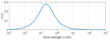
Figure 2: The dependence of visibility of phase-localization versus drive amplitude $\Omega$, showing an optimum strength at around 0.1 Hz.

IV Interferometric measurement of Husimi distribution (IMHD)

Theoretically, the instantaneous state can be directly predicted by solving the master equation, following which the Husimi function can be evaluated using Eq. (1). Experimentally, the standard way to extract Husimi distribution is by using Eq. (1) after carrying out QST to estimate the steady state density matrix $\rho$ [32]. However, there are two unrelated issues that plague tomographic measurements in quantum systems. One relates to the fact that the experimental complexity of QST scales exponentially with the system size [45, 46], each component of which has to be measured repeatedly. This introduces deleterious noise sources when multiple experiments are needed to perform QST. Having said that, for small quantum systems such as a four-level system, full tomography is routine. This leads us to the second issue, which is that even in small system sizes considered here, QST of steady states turned out to be highly inefficient. The reason being QST relies on determining each element of the density matrix via a linear combination of expectation values of a set of observables. If the expectation values vary over large magnitudes, the dynamic range problem prevents the estimation of faintest elements. The IMHD method described here avoids the dynamic range problem and directly extracts the Husimi function at each $(\theta,\phi)$ value in a single experiment without requiring the elaborate QST protocols. This allowed us to efficiently observe and quantify synchronization even after a very long drive as explained below.

The circuit diagram representing the experiment to read the Husimi Q-function values is shown in Fig. LABEL:circuit(a). Here, ¹⁹F qubit acts as the ancillary system, which along with ³¹P qubit begin from a thermal equilibrium state $\rho^{\mathrm{eq}}$. The long weak-drive responsible for synchronization is applied on the $|{2}\rangle\leftrightarrow|{4}\rangle$ transition of the ³¹P qubit. As part of the interferometer, we now apply a Hadamard operator on ¹⁹F qubit and prepare its superposition. Meanwhile, we apply the gate $U^{\dagger}_{\theta,\phi}$ on ³¹P qubit. Subsequently, we apply a controlled phase-gate $\mathbbm{1}_{P}\otimes|{0}\rangle\langle{0}|_{F}+\sigma_{z}^{P}\otimes|{1}\rangle\langle{1}|_{F}$.

Starting from the extremal state $|{0,0}\rangle=|{\theta=0,\phi=0}\rangle$, we can generate the spin coherent state

$$|{\theta,\phi}\rangle=U_{\theta,\phi}|{0,0}\rangle=\left[e^{-i\phi S_{z}}e^{-i\theta S_{y}}\otimes\mathbbm{1}^{F}\right]|{0,0}\rangle.$$ (29)

The corresponding IMHD reading is

$$Q_{\mathrm{IF}}(\theta,\phi) =\langle{\theta,\phi}|{\rho^{\mathrm{ss}}}|{\theta,\phi}\rangle=\mathrm{Tr}\left(\rho^{\mathrm{ss}}|{\theta,\phi}\rangle\langle{\theta,\phi}|\right)$$

$$=\mathrm{Tr}\left(\rho^{\mathrm{ss}}U_{\theta,\phi}|{0,0}\rangle\langle{0,0}|U_{\theta,\phi}^{\dagger}\right)$$

$$=\mathrm{Tr}\left(U_{\theta,\phi}^{\dagger}\rho^{\mathrm{ss}}U_{\theta,\phi}|{0,0}\rangle\langle{0,0}|\right)$$

$$=\langle{|{0,0}\rangle\langle{0,0}|}\rangle_{\rho_{\theta,\phi}},$$ (30)

where $\rho_{\theta,\phi}=U_{\theta,\phi}^{\dagger}\rho^{\mathrm{ss}}U_{\theta,\phi}$.

The NMR pulse sequence for IMHD is shown in Fig. LABEL:circuit(b). After the $|{2}\rangle\leftrightarrow|{4}\rangle$ drive, we implement a pseudo-Hadamard operator using a $90^{\circ}_{y}$ pulse on the ¹⁹F spin. While $U_{\theta}^{\dagger}=e^{i\theta I_{y}}$ can be realized by a single $\theta_{\bar{y}}$ pulse, $U_{\phi}^{\dagger}=e^{i\phi I_{z}}=e^{-i\frac{\pi}{2}I_{y}}e^{-i\phi I_{x}}e^{i\frac{\pi}{2}I_{y}}$ is realized by a sequence of three pulses. The measurement of $|{0,0}\rangle\langle{0,0}|$ projector can be realized via a controlled phase-gate, which can be implemented, up to a phase-factor, by a simple free evolution under the system Hamiltonian $2\pi JI_{z}^{P}I_{z}^{F}$ for a time duration of $1/2J$. A subsequent measurement of transverse magnetization of the ¹⁹F spin yields the NMR signal

$$s=\mathrm{Re}\langle{\sigma_{x}^{F}}\rangle= \frac{1}{2}\left\{C_{2\theta}\left[\rho_{11}^{\mathrm{ss}}-\rho_{22}^{\mathrm{ss}}-\rho_{33}^{\mathrm{ss}}+\rho_{44}^{\mathrm{ss}}\right]\right.$$

$$+\left.S_{2\theta}~{}\mathrm{Re}(e^{-i\phi}\rho_{24}^{\mathrm{ss}}+e^{i\phi}\rho_{42}^{\mathrm{ss}})\right\}.$$ (31)

One can verify from Eq. (II) and Eq. (31) that

$$Q_{\mathrm{IF}}(\theta,\phi) =\frac{24}{\pi^{3}}\left[\frac{1+2s}{2}-\left(\rho_{11}^{\mathrm{ss}}C^{2}_{\theta}+\rho_{33}^{\mathrm{ss}}S^{2}_{\theta}\right)\right]$$

$$=Q(\theta,\phi).$$ (32)

Here $\rho_{11}^{\mathrm{ss}}\simeq\rho_{11}^{\mathrm{eq}}$ and $\rho_{33}^{\mathrm{ss}}\simeq\rho_{33}^{\mathrm{eq}}$ are the populations of undriven levels and can be estimated from the thermal equilibrium population distribution. For the highly mixed NMR systems, $\rho_{11}\simeq\rho_{33}\simeq 1/4$, so that,

$$Q_{\mathrm{IF}}(\theta,\phi) =\frac{24}{\pi^{3}}\left[\frac{1+2s}{2}-\frac{1}{4}\right]=\frac{24}{\pi^{3}}\left[s+\frac{1}{4}\right].$$ (33)

Thus, the ¹⁹F signal after the IMHD circuit of Fig. LABEL:circuit can directly measure the Husimi distribution values. One such spectrum for a particular drive duration and $(\theta,\phi)$ values is shown in Fig. 1(f). Note that one may use a third spin as an ancilla qubit for the interferometer circuit, but it will open up additional dissipation pathways. To minimise such decoherence channels, we have used one of the system spins itself as an ancilla qubit.

V Results

The experimental IMHD results at thermal equilibrium as well as at various drive durations are shown in Fig. LABEL:results. The signal measured at the end of the IMHD circuit (Fig. LABEL:circuit) is directly used to estimate the Husimi distributions using Eq. (33). The title of each sub-figure indicates the value of the corresponding visibility factor of the Husimi distribution.

Limit cycle:

In the absence of drive, the system is in thermal equilibrium with the environment. Husimi distribution of the thermal equilibrium state $\rho^{\mathrm{eq}}$ is shown in Fig. LABEL:results (a), which is uniform throughout the phase space with no phase localization, and accordingly vanishingly small visibility factor. Therefore $\rho^{\mathrm{eq}}$ is a valid limit cycle with free phase, as is expected.

Onset of synchronization:

To study synchronization in the system, we apply a weak transition-selective drive of strength $\Omega=0.1$ Hz on-resonant with the $|{2}\rangle\leftrightarrow|{4}\rangle$ transition as shown in Fig. 1(b). The equilibration time of the quantum system is approximately 10 s, which means that dynamics captured under 10 s can be considered transient whereas for timescales much larger than 10 s we observe steady states of the system. The drive is applied for different durations which enabled us to investigate the transient and steady state dynamics in the subspace of interest. The experimentally measured Husimi distributions for various drive durations are shown in Fig. LABEL:results (a). The corresponding distributions for the instantaneous states predicted by the numerical model (described in section III.2) are shown in Fig. LABEL:results (b). We can see that the system gradually develops phase localization with the drive before reaching a steady state. For short drive durations, i.e., for 50 ms, 100 ms we observe a weak phase localization, which captures the transient dynamics. In this transient regime, the experimental phase distribution reached a peak localization strength at 1 s drive duration. The system then reaches a steady state with the phase localization stabilizing for drive durations roughly above 10 s. It remains synchronized even up till 100 s, which is more than ten times the drive period as well as ten times the $T_{1}$ relaxation time constants of the system spins.

The experimental phase localization pattern and visibility factors match fairly well with those predicted by the numerical model. While an elaborate relaxation model, accounting for all the Lindblad dissipation operators and other experimental imperfections such as RF inhomogeneity might explain the observed deviations, the current minimal model nonetheless captures the essential signatures of synchronization.

Arnold tongue:

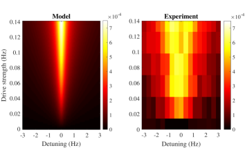
Figure 5: Arnold tongue behaviour of the system. The system shows strongest synchronization for on-resonant drive and strong drive strengths, while off-resonant drives are unable to synchronize with the transition of interest even for large driving strengths.

Arnold tongue is a quintessential test of synchronization that probes robustness of phase-localization against small changes in drive strengths and drive detuning [1]. As the drive strength is increased, the region of synchronization can be shown to be wider, leading to the familiar “tongue” shape. Here, we vary the drive strength of the 100 s weak drive, and its resonance-offset by 3 Hz about the resonance value. The Arnold tongue is quantified using the maximum of the synchronization measure, $\max\left[S(\phi)\right]$, and in the present case it is only dependent on the $\rho_{42}$ element of the density matrix, as evident from Eq. (13). Experimentally, this can be directly measured from the intensity of ³¹P NMR spectrum (see Fig. 1(e)). Fig. 5 compares the result of the Arnold tongue experiments with that of the numerical prediction (from the model described in section III.2). For strong drive strength and near resonance conditions, the degree of synchronization is higher since the drive has more efficient perturbative effect on the system. On the other hand, for larger detuning and weaker drives, the extent of synchronization is weaker. Despite an overall correspondence between the experimental and the predicted profiles, we see a higher spread along the detuning axis in the experimental data, which can be attributed to the limitations of the minimal numerical model and experimental imperfections.

VI Summary and Outlook

Recently there has been an increasing interest in studying the synchronization of quantum systems with external drives under suitable conditions. In this work, we experimentally demonstrated synchronization in a two-qubit system using NMR architecture. We use the Husimi distribution function as a witness for synchronization. We applied a weak transition selective drive on one of the spins and observed the gradual onset of phase-localization via Husimi distribution. In the absence of any external drive, the system evolves under its internal Hamiltonian as well as inherent relaxation mechanisms, thereby settling to its thermal equilibrium state. The corresponding Husimi distribution pattern has no phase-preference, and hence the thermal equilibrium state forms the valid limit cycle of the system.

An interesting issue that arises with the study of steady state dynamics of open quantum systems relates to the fact that NMR signals are proportional to the population differences. Since the populations are in a pseudo-spin state, their effective difference dips below the noise threshold, rendering steady state population tomography difficult in such systems until now. Here we reported an interferometric technique to directly extract the Husimi distribution values by reading the signal of the undriven spin. The interferometric method is significantly more efficient compared to the standard method based on quantum state tomography.

To establish the robustness of synchronization, we investigated the response of the system to changes in drive strengths and drive detuning. The resulting phase-localization measure of the system exhibited the expected Arnold tongue behaviour. We compared the experimental results with a minimalistic $T_{1}$ relaxation model of the two-qubit nuclear spin system, which could capture the general features of the experimental data.

This work demonstrates the suitability of NMR architecture for quantum synchronization studies and also opens up avenues for further exploration of the phenomenon in larger spin systems as well as under a variety of interactions and drive conditions. One can envisage NMR systems being useful for studying the implications of synchronization in areas such as spectroscopy, quantum computing and quantum thermodynamics.

Appendix A Spin coherent states

Spin coherent states are routinely used to study synchronization since their evolutions are closest to classical trajectories [47]. Furthermore, coherent states exhibit stable oscillations as explained below. For a spin-1/2 particle, the $z$ projection of the spin angular momentum $S_{z}$ is quantized into 2s+1 levels $|{S,m_{s}}\rangle$ with eigenvalues $m_{s}=-1/2,1/2$. The spin coherent state for this spin in SU(2) group can be described as a rotation of the extremal state $|{S,S}\rangle$ such that [48, 49, 36]

$$|{\hat{n}_{2}}\rangle=|{\theta,\phi}\rangle=\mathrm{e}^{-i\phi S_{z}}\mathrm{e}^{-i\theta S_{y}}|{S,S}\rangle=\left(\begin{array}[]{c}C_{\theta_{1}}\\ e^{i\phi}S_{\theta_{1}}\end{array}\right),$$ (36)

where $\theta\in[0,\pi]$, $\phi\in[0,2\pi]$, $C_{\theta}=\cos(\theta/2)$, and $S_{\theta}=\sin(\theta/2)$. It is obvious that spin-1/2 coherent states can be mapped to points on the surface of the Bloch sphere. The recursive construction of spin coherent state vectors for an $n$-level non-degenerate system is [36, 35]

$$|{\hat{n}_{n}}\rangle=\left(\begin{array}[]{c}C_{\theta}\\ 0\\ \vdots\\ 0\end{array}\right)+e^{i\phi}S_{\theta}\left(\begin{array}[]{c}0\\ \\ |{\hat{n}_{n-1}}\rangle\\ \\ \end{array}\right).$$ (45)

Note that each lower-level vector $|{\hat{n}_{n-1}}\rangle$ is made up of a new pair of angular variables. From the above, we obtain the $SU(4)$ coherent states in the form

$$|{\hat{n}_{4}}\rangle=\left(\begin{array}[]{c}C_{\theta_{1}}\\ e^{i\phi_{1}}S_{\theta_{1}}C_{\theta_{2}}\\ e^{i\phi_{2}}S_{\theta_{1}}S_{\theta_{2}}C_{\theta_{3}}\\ e^{i\phi_{3}}S_{\theta_{1}}S_{\theta_{2}}S_{\theta_{3}}\end{array}\right).$$ (50)

From the above definition, we can see that populations are governed by the parameters $(\theta_{1},\theta_{2},\theta_{3})$, and phases by the parameters $(\phi_{1},\phi_{2},\phi_{3})$.

Appendix B Lindblad relaxation operators

The explicit form of the single-quantum jump operators considered for the four-level system shown in Fig. 1(b) are explained here. The single-quantum transition of the first qubit implies that the system in a state $|{i}\rangle|{j}\rangle$ goes to the state $|{k}\rangle|{l}\rangle$, where $k=i\pm 1$, and $l=j$. The same can be extended to the single-quantum transition of the second qubit. The Lindblad superoperator for upward transitions of the combined two-qubit system is hence given by $\mathcal{D}[\hat{O}_{+}]\rho=\sum_{(k-i=1,l=j)}D[\mathcal{O}_{ij}^{kl}]\rho+\sum_{(k=i,l-j=1)}D[\mathcal{O}_{ij}^{kl}]\rho$ where $D[\hat{\mathcal{O}}]\rho=\hat{\mathcal{O}}\rho\hat{\mathcal{O}}^{\dagger}-\{\hat{\mathcal{O}}^{\dagger}\hat{\mathcal{O}},\rho\}/2$ and jump operator $\mathcal{O}_{ij}^{kl}$ is defined as $\mathcal{O}_{ij}^{kl}=\sqrt{g_{ij}^{kl}p_{ij}^{kl}}~{}|{k}\rangle|{l}\rangle\langle{i}|\langle{j}|$. Similarly, we can write $\mathcal{D}[\hat{O}_{-}]\rho=\sum_{(k-i=1,l=j)}D[\mathcal{O}^{ij}_{kl}]\rho+\sum_{(k=i,l-j=1)}D[\mathcal{O}^{ij}_{kl}]\rho$, where $\mathcal{O}^{ij}_{kl}=(\mathcal{O}_{ij}^{kl})^{\dagger}$. The coefficients of the jump operators corresponding to each qubit determine the transition rate given by $g_{ij}^{kl}$, and the transition probability given by $p_{ij}^{kl}$. The transition rate is dependent on the bath temperature via spin-lattice relaxation time constant $T_{1}$, and the transition probabilities are derived from a fermionic bath model, as explained in the main text.

Appendix C Very low power RF calibration

As discussed in section III.3, observation of phase-synchronization requires a drive of amplitude $10^{-1}$ Hz. The calibration of such very weak RF is nontrivial, since the signal to noise ratio is negligibly small. For this purpose, we used another spin-system trimethylphosphite dissolved in dimethylsulphoxide solvent. We specifically chose this sample because of its star-topology with ³¹P at the centre coupled to nine identical ¹H nuclei with a scalar J coupling constant of 11 Hz, as shown in Fig. LABEL:tmp. Such geometry is highly preferable since the magnetization of the nine high $\gamma$ proton nuclei can be easily transferred to the central ³¹P nucleus via INEPT and further algorithmic cooling, thus boosting its signal [50]. This gives better signal to noise ratio and hence more accurate calibration values. For very low amplitudes, the signal $\propto\sin(\Omega t)\approxeq\Omega t$, and therefore we expect a linear dependence. The calibration results are shown in Fig. LABEL:lowpowercalib. As we can see, the intensity of the ³¹P spectrum after decoupling protons varies linearly with time for the low amplitude pulses. Thus by fitting a linear function to the resulting curve, we can back-calculate the exact amplitude of the pulse. The estimated and exact values from back calculation of the linear fit are shown in the legend. These low power pulses were used in the Husimi distribution estimation and Arnold tongue experiments.

References

- Pikovsky et al. [2003] A. Pikovsky, J. Kurths, M. Rosenblum, and J. Kurths, Synchronization: a universal concept in nonlinear sciences, 12 (Cambridge university press, 2003).
- Lee and Sadeghpour [2013] T. E. Lee and H. R. Sadeghpour, Quantum synchronization of quantum van der pol oscillators with trapped ions, Physical review letters 111, 234101 (2013).
- Hush et al. [2015] M. R. Hush, W. Li, S. Genway, I. Lesanovsky, and A. D. Armour, Spin correlations as a probe of quantum synchronization in trapped-ion phonon lasers, Physical Review A 91, 061401 (2015).
- Nigg [2018] S. E. Nigg, Observing quantum synchronization blockade in circuit quantum electrodynamics, Physical Review A 97, 013811 (2018).
- Xu et al. [2014] M. Xu, D. A. Tieri, E. C. Fine, J. K. Thompson, and M. J. Holland, Synchronization of two ensembles of atoms, Physical review letters 113, 154101 (2014).
- Ludwig and Marquardt [2013] M. Ludwig and F. Marquardt, Quantum many-body dynamics in optomechanical arrays, Phys. Rev. Lett. 111, 073603 (2013).
- Walter et al. [2014] S. Walter, A. Nunnenkamp, and C. Bruder, Quantum synchronization of a driven self-sustained oscillator, Physical review letters 112, 094102 (2014).
- Walter et al. [2015] S. Walter, A. Nunnenkamp, and C. Bruder, Quantum synchronization of two van der pol oscillators, Annalen der Physik 527, 131 (2015).
- Li et al. [2016] W. Li, C. Li, and H. Song, Quantum synchronization in an optomechanical system based on lyapunov control, Physical Review E 93, 062221 (2016).
- Zhang et al. [2012] M. Zhang, G. S. Wiederhecker, S. Manipatruni, A. Barnard, P. McEuen, and M. Lipson, Synchronization of micromechanical oscillators using light, Physical review letters 109, 233906 (2012).
- Holmes et al. [2012] C. A. Holmes, C. P. Meaney, and G. J. Milburn, Synchronization of many nanomechanical resonators coupled via a common cavity field, Physical Review E 85, 066203 (2012).
- Witthaut et al. [2017] D. Witthaut, S. Wimberger, R. Burioni, and M. Timme, Classical synchronization indicates persistent entanglement in isolated quantum systems, Nature communications 8, 1 (2017).
- Roulet and Bruder [2018a] A. Roulet and C. Bruder, Quantum synchronization and entanglement generation, Physical review letters 121, 063601 (2018a).
- Jaseem et al. [2020a] N. Jaseem, M. Hajdušek, V. Vedral, R. Fazio, L.-C. Kwek, and S. Vinjanampathy, Quantum synchronization in nanoscale heat engines, Physical Review E 101, 020201 (2020a).
- Solanki et al. [2021] P. Solanki, N. Jaseem, M. Hajdušek, and S. Vinjanampathy, Role of coherence and degeneracies in quantum synchronisation, arXiv preprint arXiv:2104.04383 (2021).
- Li et al. [2017a] W. Li, C. Li, and H. Song, Quantum synchronization and quantum state sharing in an irregular complex network, Physical Review E 95, 022204 (2017a).
- Hajdušek et al. [2021] M. Hajdušek, P. Solanki, R. Fazio, and S. Vinjanampathy, Seeding crystallization in time, arXiv preprint arXiv:2111.04395 (2021).
- Schleich [2011] W. P. Schleich, Quantum optics in phase space (John Wiley & Sons, 2011).
- Galve et al. [2017] F. Galve, G. Luca Giorgi, and R. Zambrini, Quantum correlations and synchronization measures, in Lectures on General Quantum Correlations and their Applications (Springer International Publishing, Cham, 2017) pp. 393–420.
- Li et al. [2017b] W. Li, W. Zhang, C. Li, and H. Song, Properties and relative measure for quantifying quantum synchronization, Physical Review E 96, 012211 (2017b).
- Koppenhöfer and Roulet [2019] M. Koppenhöfer and A. Roulet, Optimal synchronization deep in the quantum regime: Resource and fundamental limit, Physical Review A 99, 043804 (2019).
- Mari et al. [2013] A. Mari, A. Farace, N. Didier, V. Giovannetti, and R. Fazio, Measures of quantum synchronization in continuous variable systems, Phys. Rev. Lett. 111, 103605 (2013).
- Jaseem et al. [2020b] N. Jaseem, M. Hajdušek, P. Solanki, L.-C. Kwek, R. Fazio, and S. Vinjanampathy, Generalized measure of quantum synchronization, Physical Review Research 2, 043287 (2020b).
- Manzano et al. [2013] G. Manzano, F. Galve, G. L. Giorgi, E. Hernández-García, and R. Zambrini, Synchronization, quantum correlations and entanglement in oscillator networks, Scientific Reports 3, 1 (2013).
- Ameri et al. [2015] V. Ameri, M. Eghbali-Arani, A. Mari, A. Farace, F. Kheirandish, V. Giovannetti, and R. Fazio, Mutual information as an order parameter for quantum synchronization, Physical Review A 91, 012301 (2015).
- Roulet and Bruder [2018b] A. Roulet and C. Bruder, Synchronizing the smallest possible system, Phys. Rev. Lett. 121, 053601 (2018b).
- Sonar et al. [2018] S. Sonar, M. Hajdušek, M. Mukherjee, R. Fazio, V. Vedral, S. Vinjanampathy, and L.-C. Kwek, Squeezing enhances quantum synchronization, Phys. Rev. Lett. 120, 163601 (2018).
- Buca et al. [2021] B. Buca, C. Booker, and D. Jaksch, Algebraic theory of quantum synchronization and limit cycles under dissipation, arXiv preprint arXiv:2103.01808 (2021).
- Koppenhöfer et al. [2020] M. Koppenhöfer, C. Bruder, and A. Roulet, Quantum synchronization on the ibm q system, Physical Review Research 2, 023026 (2020).
- Laskar et al. [2020] A. W. Laskar, P. Adhikary, S. Mondal, P. Katiyar, S. Vinjanampathy, and S. Ghosh, Observation of quantum phase synchronization in spin-1 atoms, Physical Review Letters 125, 013601 (2020).
- Bengtsson and Zyczkowski [2006] I. Bengtsson and K. Zyczkowski, Geometry of Qauntum States: An Introduction to Quantum Entanglement (Cambridge University Press, 2006).
- Krithika et al. [2019] V. R. Krithika, V. S. Anjusha, U. T. Bhosale, and T. S. Mahesh, Nmr studies of quantum chaos in a two-qubit kicked top, Physical Review E 99, 032219 (2019).
- Husimi [1940] K. Husimi, Some formal properties of the density matrix, Proceedings of the Physico-Mathematical Society of Japan. 3rd Series 22, 264 (1940).
- Kano [1965] Y. Kano, A new phase-space distribution function in the statistical theory of the electromagnetic field, Journal of Mathematical Physics 6, 1913 (1965).
- Perelomov [1986] A. Perelomov, Generalized Coherent States and Their Applications (Springer, Berlin, Heidelberg, 1986).
- Nemoto [2000] K. Nemoto, Generalized coherent states for su (n) systems, Journal of Physics A: Mathematical and General 33, 3493 (2000).
- Mathur and Mani [2002] M. Mathur and H. Mani, Su (n) coherent states, Journal of Mathematical Physics 43, 5351 (2002).
- Breuer et al. [2002] H.-P. Breuer, F. Petruccione, et al., The theory of open quantum systems (Oxford University Press on Demand, 2002).
- Ghosh et al. [2012] A. Ghosh, S. S. Sinha, and D. S. Ray, Fermionic oscillator in a fermionic bath, Physical Review E 86, 011138 (2012).
- Suri et al. [2018] N. Suri, F. C. Binder, B. Muralidharan, and S. Vinjanampathy, Speeding up thermalisation via open quantum system variational optimisation, The European Physical Journal Special Topics 227, 203 (2018).
- Manzano [2020] D. Manzano, A short introduction to the lindblad master equation, AIP Advances 10, 025106 (2020).
- Gyamfi [2020] J. A. Gyamfi, Fundamentals of quantum mechanics in liouville space, European Journal of Physics 41, 063002 (2020).
- Navarrete-Benlloch [2015] C. Navarrete-Benlloch, Open systems dynamics: Simulating master equations in the computer, arXiv preprint arXiv:1504.05266 (2015).
- Boulant et al. [2003] N. Boulant, T. F. Havel, M. A. Pravia, and D. G. Cory, Robust method for estimating the lindblad operators of a dissipative quantum process from measurements of the density operator at multiple time points, Physical Review A 67, 042322 (2003).
- Chuang et al. [1998] I. L. Chuang, N. Gershenfeld, M. G. Kubinec, and D. W. Leung, Bulk quantum computation with nuclear magnetic resonance: theory and experiment, Proceedings of the Royal Society of London. Series A: Mathematical, Physical and Engineering Sciences 454, 447 (1998).
- Shukla et al. [2013] A. Shukla, K. R. K. Rao, and T. S. Mahesh, Ancilla-assisted quantum state tomography in multiqubit registers, Physical Review A 87, 062317 (2013).
- Lee Loh and Kim [2015] Y. Lee Loh and M. Kim, Visualizing spin states using the spin coherent state representation, American Journal of Physics 83, 30 (2015).
- Radcliffe [1971] J. Radcliffe, Some properties of spin coherent states, Phys. A: Math. Gen 4, 313 (1971).
- Klauder and Skagerstam [1985] J. R. Klauder and B. Skagerstam, Coherent Sattes:Applications in Physics and Mathematical Physics (World Scientific, 1985).
- Pande et al. [2017] V. R. Pande, G. Bhole, D. Khurana, and T. S. Mahesh, Strong algorithmic cooling in large star-topology quantum registers, Phys. Rev. A 96, 012330 (2017).