Barely-Supervised Learning:
Semi-Supervised Learning with very few labeled images

Abstract

This paper tackles the problem of semi-supervised learning when the set of labeled samples is limited to a small number of images per class, typically less than 10, problem that we refer to as barely-supervised learning. We analyze in depth the behavior of a state-of-the-art semi-supervised method, FixMatch, which relies on a weakly-augmented version of an image to obtain supervision signal for a more strongly-augmented version. We show that it frequently fails in barely-supervised scenarios, due to a lack of training signal when no pseudo-label can be predicted with high confidence. We propose a method to leverage self-supervised methods that provides training signal in the absence of confident pseudo-labels. We then propose two methods to refine the pseudo-label selection process which lead to further improvements. The first one relies on a per-sample history of the model predictions, akin to a voting scheme. The second iteratively updates class-dependent confidence thresholds to better explore classes that are under-represented in the pseudo-labels. Our experiments show that our approach performs significantly better on STL-10 in the barely-supervised regime, e.g. with 4 or 8 labeled images per class.

1 Introduction

While early deep learning methods have reached outstanding performance in fully-supervised settings (Krizhevsky, Sutskever, and Hinton 2012; Simonyan and Zisserman 2015; He et al. 2016), a recent trend is to focus on reducing this need for labeled data. Self-supervised models take it to the extreme by learning models without any labels; in particular recent works based on the paradigm of contrastive learning (He et al. 2020; Chen et al. 2020a; Grill et al. 2020; Caron et al. 2020), learn features that are invariant to class-preserving augmentations and have shown transfer performances that sometimes surpass that of models pretrained on ImageNet with label supervision. In practice, however, labels are still required for the transfer to the final task. Semi-supervised learning aims at reducing the need for labeled data in the final task, by leveraging both a small set of labeled samples and a larger set of unlabeled samples from the target classes. In this paper, we study the case of semi-supervised learning when the set of labeled samples is reduced to a very small number, typically 4 or 8 per class, which we refer to as barely-supervised learning.

The recently proposed FixMatch approach (Sohn et al. 2020) unifies two trends in semi-supervised learning: pseudo-labeling (Lee 2013) and consistency regularization (Bachman, Alsharif, and Precup 2014; Rasmus et al. 2015). Pseudo-labeling, also referred to as self-training, consists in accepting confident model predictions as targets for previously unlabeled images, as if they were true labels. Consistency regularization methods obtain training signal using a modified version of an input, e.g. using another augmentation, or a modified version of the model being trained. In FixMatch, a weakly-augmented version of an unlabeled image is used to obtain a pseudo-label as distillation target for a strongly-augmented version of this same image. In practice, the pseudo-label is only set if the prediction is confident enough, as measured by the peakiness of the softmax predictions. If no confident prediction can be made, no loss is applied to the image sample. FixMatch obtains state-of-the-art semi-supervised results, and was the first to demonstrate performance in barely-supervised learning close to fully-supervised methods on CIFAR-10. However, it does not perform as well with more realistic images, e.g. on the STL-10 dataset when the set of labeled images is small.

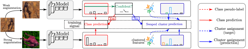
Figure 1: Overview of our approach. Given one weak and one strong augmentation of one unlabeled image, we look at the prediction of the weak augmentation. If it is confident, we use it to obtain a pseudo-label which is used for supervision of the strong augmentation. Otherwise, we use feature cluster assignments as target while FixMatch discards the data point.

In this paper, we first analyze the causes that hurt performance in this regime. In practice, we find the choice of confidence threshold, beyond which a prediction is accepted as pseudo-label, to have a high impact on performance. A high threshold leads to pseudo-labels that are more likely to be correct, but also to fewer unlabeled images being considered. Thus in practice a smaller subset of the unlabeled data receives training signal, and the model may not be able to make high quality predictions outside of it. If the threshold is set too low, many images will receive pseudo-labels but with the risk of using wrong labels, that may then propagate to other images, a problem known as confirmation bias (Arazo et al. 2020). In other words, FixMatch faces a distillation dilemma between allowing more exploration but with possibly noisy labels, or exploring fewer images with more chances to have correct pseudo-labels.

For barely-supervised learning, a possibility is to leverage a self-then-semi paradigm, i.e., to first train a model with self-supervision then with semi-supervised learning, as proposed in SelfMatch (Kim et al. 2020). We find that this might not be optimal as the self-supervision step ignores the availability of labels for some images. Empirically, we observe that such models tend to output overconfident pseudo-labels in early training, including for incorrect predictions.

In this paper, we propose a simple solution to unify self- and semi-supervised strategies, mainly by using a self-supervision signal in cases where no pseudo-label can be assigned with high confidence, see Figure 1 for an overview. Specifically, we perform online deep-clustering  (Caron et al. 2020) and enforce consistency between predicted cluster assignments for two augmented versions of an image when pseudo-labels are not confident. This simple algorithmic change leads to clear empirical benefits for barely-supervised learning, owing to the fact that training signal is available even when no pseudo-label is assigned. We further propose two strategies to refine pseudo-label selection: (a) by leveraging the history of the model prediction per sample and (b) by imposing constraints on the ratio of pseudo-labeled samples per class. We refer to our method as LESS, for label-efficient semi-supervision. Our experiments demonstrate substantial benefits from using our approach on STL-10 in barely-supervised settings. For instance, test accuracy increases from 35.8% to 64.2% when considering 4 labeled images per class, compared to FixMatch. We also improve over other baselines that employ self-supervised learning as pretraining, followed by FixMatch.
Summary of our main contributions:

• An analysis of the distillation dilemma in FixMatch. We show that it leads to failures with very few labels.

• A semi-supervised learning method which provides training signal in the absence of pseudo-labels and two methods to refine the quality of pseudo-labels.

• Experiments showing that our approach allows barely-supervised learning on the more realistic STL-10 dataset.

This paper starts with a review of the related work (Section 2), then we analyze the distillation dilemma of FixMatch in Section 3. We propose our method for bare supervision in Section 4 and our experimental results in Section 5.

2 Related work

In this section, we first briefly review related work on semi-supervised learning (Section 2.1) and self-supervised learning (Section 2.2). Section 2.3 finally discusses recent works that leverage both self- and semi-supervision.

2.1 Semi-Supervised Learning

Self-training is a popular method for semi-supervised learning where model predictions are used to provide training signal for unlabeled data, see (Xie et al. 2020; Lee 2013; Zhang and Sabuncu 2020). In particular, Pseudo-labeling (Lee 2013) generates artificial labels in the form of hard assignments, typically when a given measure of model confidence, such as the peakiness of the predicted probability distribution, is above a certain threshold (Rosenberg, Hebert, and Schneiderman 2005). Note that this results in the absence of training signal when no confident prediction can be made. In (Pham et al. 2021), a teacher network is trained with reinforcement learning to provide a student network with pseudo-labels that improve its performance. Consistency regularization (Bachman, Alsharif, and Precup 2014; Rasmus et al. 2015; Sajjadi, Javanmardi, and Tasdizen 2016) is based on the assumption that model predictions should not be sensitive to perturbations applied on the input samples. Several predictions are considered for a given data sample, for instance using multiple augmentations or different versions of the trained model. Artificial targets are then provided by enforcing consistency across these different outputs. This objective can be used as a regularizer, computed on the unlabeled data along with a supervised objective.

ReMixMatch (Berthelot et al. 2019a) and Unsupervised Data Augmentation (Xie et al. 2019) (UDA) have shown impressive results by using model predictions on weakly-augmented version of an image to generate artificial target probability distributions. These distributions are then sharpened and used as supervision for a strongly-augmented version of the same image. FixMatch (Sohn et al. 2020) provides a simplified version where pseudo-labeling is used instead of distribution sharpening, without the need for additional tricks such as distribution alignment or augmentation anchoring (i.e., using more than one weak and one strong augmented version) from ReMixMatch or training signal annealing from UDA. Additionally, similar unlabeled images can be encouraged to have consistent pseudo-labels (Hu, Yang, and Nevatia 2021), or pseudo-labels can be propagated via a similarity graph (Li et al. 2020) or centroids (Han et al. 2021). Our method extends FixMatch by leveraging a self-supervised loss in cases where the pseudo-label is unconfident, allowing to perform barely-supervised learning in realistic settings.

2.2 Self-Supervised Learning

Early works such as (Doersch, Gupta, and Efros 2015; Dosovitskiy et al. 2014; Gidaris, Singh, and Komodakis 2018; Noroozi and Favaro 2016) on self-supervised learning were based on the idea that a network could learn important image features and semantic representation of the scenes when trained to predict basic transformations applied to the input data, such as a simple rotation in RotNet (Gidaris, Singh, and Komodakis 2018) or solving a jigsaw puzzle of an image  (Noroozi and Favaro 2016), i.e., recovering the original position of the different pieces. More recently, impressive results have been obtained using contrastive learning (Wu et al. 2018a, b; Chen et al. 2020a, c), to the point of outperforming supervised pretraining for tasks such as object detection, at least when performing the self-supervision on object-centric datasets (Purushwalkam and Gupta 2020) such as ImageNet. The main idea consists in learning feature invariance to class-preserving augmentations. More precisely, each batch contains multiple augmentations of a set of images and the network should output features that are close for variants of a same image and far from those from the other images. In other words, it corresponds to learning instance discrimination, and is closely related to consistency regularization. Reviewing the literature on this topic is beyond the scope of this paper. Major directions consist in studying the type of augmentation being performed (Asano, Rupprecht, and Vedaldi 2020; Gontijo-Lopes et al. 2020; Tian et al. 2020), adapting batch normalisation statistics (Cai et al. 2021), the way to provide hard negatives with for instance a queue (He et al. 2020; Chen et al. 2020c) or large batch size (Chen et al. 2020a), or even questioning the need for these negatives (Chen and He 2021; Grill et al. 2020). With online deep-clustering (Caron et al. 2020), the feature invariance principle is slightly relaxed by learning to predict cluster assignments, i.e., encouraging features of different augmentations of an image to be assigned to the same cluster, but not necessarily to be exactly similar.

2.3 Combination of self-supervised and semi-supervised learning

In SelfMatch (Kim et al. 2020), the authors propose to apply a state-of-the-art semi-supervised method (FixMatch) starting from a model pretrained with self-supervision using SimCLR (Chen et al. 2020a). Similarly, CoMatch (Li, Xiong, and Hoi 2021) shows that using such a model for initialization performs slightly better than using a randomly initialized network, and (Lerner, Shiran, and Weinshall 2020) alternate between self- and semi-supervised training. In this paper, we depart from the sequential approach of doing self-supervision followed by semi-supervision, with a tighter connection between the two concepts, and empirically demonstrate that it leads to improved performance. Chen et al. (2020b) have proposed another strategy where the self-supervision is first applied, then a classifier is learned on the labeled samples only, which is used to assign a pseudo-label to each unlabeled sample. These pseudo-labels are finally used for training a classifier on all samples. While impressive results are shown on ImageNet with 1% of the training data, it still represents about 13,000 labeled samples, and may generalize less when considering a lower number of labeled examples. S4L (Zhai et al. 2019) used a multi-task loss where a self-supervised loss is applied to all samples while a supervised loss is additionally applied to labeled samples only. Similarly to (Chen et al. 2020b), the classifier is only learned on the labeled samples, a scenario which would fail in the regime of bare supervision where very few labeled samples are considered.

3 The distillation dilemma in FixMatch

In this section, we first introduce FixMatch in more details (Section 3.1) and then formalize the dilemma between exploration vs. pseudo-label accuracy (Section 3.2).

3.1 The FixMatch method

Let $\mathcal{S}=\{(\bm{x}_{i},y_{i})\}_{i=1,\ldots M_{s}}$ be a set of labeled data, sampled from $P_{\bm{x},y}$. In fully-supervised training, the end goal is to learn the optimal parameter $\theta^{*}$ for a model $p_{\theta}$, trained to maximize the log-likelihood of predicting the correct ground-truth target, $p_{\theta}(y|\bm{x})$, given the input $\bm{x}$:

$$\theta^{*}=\operatorname*{arg\,max}_{\theta}\underset{(\bm{x},y)\sim P_{\bm{x},y}}{\mathbb{E}}\Big{[}\log p_{\theta}(y|\bm{x})\Big{]}.$$ (1)

In semi-supervised learning, an additional unlabeled set $\mathcal{U}=\{(\bm{x}_{j})\}_{j=1,\ldots M_{u}}$, where $y$ is not observed, can be leveraged.

Self-training (Yarowsky 1995) exploits unlabeled data points using model outputs as targets. Specifically, class predictions with enough probability mass (over a threshold $\tau$) are considered confident and converted to one-hot targets, called pseudo-labels. Denote the stop-gradient operator $\bar{f}$, $\hat{y}_{x}=\operatorname*{arg\,max}(\bm{\bar{p}_{\theta}}(\bm{x}))$ and $\llbracket\cdot\rrbracket$ the Iverson bracket gives:

$$\underset{\theta}{\text{maximize}}\>\>\underset{\bm{x}\sim P_{x}}{\mathbb{E}}\big{[}\>\llbracket\max\bm{\bar{p}_{\theta}}(\bm{x})\geq\tau\rrbracket\cdot\log p_{\theta}(\hat{y}_{x}|\bm{x})\>\big{]}.$$ (2)

Ideally, labels should progressively propagate to all $\bm{x}\in\mathcal{U}$.

Consistency regularization is another paradigm which assumes a family of data augmentations $\mathcal{A}$ that leaves the model target unchanged. Denote by $f_{\theta}(\bm{x})$ a feature vector, possibly different from $p_{\theta}$, e.g. produced by an intermediate layer of the network. The features produced for two augmentations of the same image are optimized to be similar, as measured by some function $\mathcal{D}$. Let $(v,w)\in\mathcal{A}^{2}$ and denote $\bm{x_{v}}=v(\bm{x})$, the objective can be written:

$$\mathcal{L}_{\text{coreg}}^{\theta}(\bm{x}_{w},\bm{x}_{v})=\>\mathcal{D}\big{[}f_{\theta}(\bm{x}_{v}),f_{\theta}(\bm{x}_{w})\big{]}.$$ (3)

This problem admits constant functions as trivial solutions; numerous methods exist to ensure that relevant information is retained (Wu et al. 2018a; Chen et al. 2020a; Caron et al. 2020; Grill et al. 2020; He et al. 2020; Wu et al. 2018b).

FixMatch. In the FixMatch algorithm, self-training and consistency-regularization coalesce in a single training loss. Weak augmentations $w\sim\mathcal{A}_{\text{weak}}$ are applied to unlabeled images, confident predictions are kept as pseudo-labels and compared with model predictions on a strongly augmented variant of the image, using $s\sim\mathcal{A}_{\text{strong}}$:

$$\mathcal{L}_{\text{distill}}^{\theta}(\bm{x}_{w},\bm{x}_{s})=\llbracket\max\bm{\bar{p}_{\theta}}(\bm{x_{w}})\geq\tau\rrbracket\cdot\log p_{\theta}(\hat{y}_{x_{w}}|\bm{x_{s}}).\vspace*{0cm}$$ (4)

3.2 Formalizing the distillation dilemma

The FixMatch algorithm (Sohn et al. 2020) has proven successful in learning an image classifier with bare supervision on CIFAR-10. As we show experimentally, it is not straightforward to replicate such performance on more challenging datasets such as STL-10. We now formalize the failure regimes of the FixMatch method.

Error drift. Assume model $p_{\theta}$ is trained with the loss in Eq. 4, and consider the event $E_{\theta}(\bm{x},\tau)$ defined as: ‘the model $p_{\theta}$ confidently make an erroneous prediction on $\bm{x}$ with confidence threshold $\tau$’, then $P(E_{\theta}(\bm{x},\tau))$ is equal to :

$$\underset{w\sim\mathcal{A}_{\text{weak}}}{\mathbb{E}}\big{[}\llbracket\max\bm{\bar{p}_{\theta}}(\bm{x}_{w})\geq\tau\rrbracket\cdot\llbracket\operatorname*{arg\,max}\bm{\bar{p}_{\theta}}(\bm{x}_{w})\neq y\rrbracket\big{]}.$$ (5)

For fixed model parameters $\theta$, $P(E_{\theta}(\bm{x},\tau))$ is monotonously decreasing in $\tau$. Denote $\theta(t)$ the model parameters at iteration $t$; If the event $E_{\theta(t)}(\bm{x},\tau)$ occurs at time $t$, by definition optimizing Equation 4 leads in expectation to $P(E_{\theta(t+1)}(\bm{x},\tau))\geq P(E_{\theta(t)}(\bm{x},\tau)).$ Thus the model becomes more likely to make the same mistake. Once the erroneous label is accepted, it can propagate to data points similar to $\bm{x}$, as happens with ground-truth targets. We refer to this phenomenon as error drift, also referred to as confirmation bias (Arazo et al. 2020). It is highlighted on the left plot of Figure 2 where the ratio of correct and confident pseudo-label drops at some point when too many incorrect pseudo-labels were used in previous iterations.

Signal scarcity. Let $r_{\theta}(\tau)$ be the expected proportion of points that do not receive a pseudo-label when using Eq. 4:

$$r_{\theta}(\tau)=\underset{\bm{x}\sim P_{x}}{\mathbb{E}}\llbracket\max\bm{\bar{p}_{\theta}}(\bm{x})<\tau\rrbracket.$$ (6)

For fixed model parameters $\theta$, $r_{\theta}(\tau)$ is monotonously increasing in $\tau$. With few ground-truth labels, most unlabelled images will be too dissimilar to any labeled one to obtain confident pseudo-labels early in training. Thus for high values of $\tau$, $r_{\theta}(\tau)$ will be close to $1$ and most data points masked by $\llbracket.\geq\tau\rrbracket$ in Equation 4, thus providing no gradient. The network receives scarce training signal; in the worst cases training will never start, or plateau early. We refer to this problem as signal scarcity. This is illustrated in Figure 2 on the right plot where the ratio of images with confident pseudo-label remains low, meaning that many unlabeled images are actually not used during training.

The distillation dilemma. We now argue that the success of the FixMatch algorithm hinges on its ability to navigate the pitfalls of error drift and signal scarcity. Erroneous predictions, as measured by $P(E_{\theta}(\bm{x},\tau))$, are avoided by increasing the hyper-parameter $\tau$. Thus the set of values that avoid error drift can be assumed of the form $\nabla=[\tau_{d},1]$ for some $\tau_{d}\in[0,1]$. Conversely avoiding signal scarcity, as measured by $r_{\theta}(\tau)$, requires reducing $\tau$, and the set of admissible values can be assumed of the form $\Delta=[0,\tau_{s}]$ for some $\tau_{s}\in[0,1]$. Successful training with Equation 4 requires the existence of a suitable value of $\tau$, i.e., $\Delta\cap\nabla\neq\varnothing$, and that this $\tau$ can be found in practice. On CIFAR-10 strikingly low amounts of labels are needed to achieve that (Sohn et al. 2020). However we show that it is not the case on more challenging datasets such as STL-10, see Figure 2.

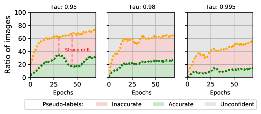
Figure 2: Illustration of the distillation dilemma of FixMatch when training on STL-10 with $40$ labels during the first $70$ epochs. For three different values of the confidence threshold $\tau$ (0.95, 0.98 and 0.995 from left to right), we show the ratio of images with a correct and confident pseudo-label (green area in bottom), with an incorrect but confident pseudo-label (red area in middle) and with unconfident pseudo-label (gray area on top) for which no training signal is used. A large value of $\tau$ leads to too few images having a pseudo-label. A lower value allows to leverage more images, but many pseudo-labels are wrong, which is emphasized in later iterations (highlighted between vertical dashed red lines for $\tau=0.95$).

4 Proposed method

In this section, we introduce our method to overcome the distillation dilemma (Section 4.1) and introduce two improvements for selecting pseudo-labels (Section 4.2).

4.1 Alleviating the distillation dilemma

In FixMatch, the absence of confident pseudo-labels leads to the absence of training signal, which is at odds with the purpose of consistency regularization - to allow training in the absence of supervision signal - and leads to the distillation dilemma. We propose instead to decouple self-training and consistency-regularization, by using self-supervision in case no confident pseudo-label has been assigned. While still relying on consistency regularization, the self-supervision does not depend at all on the labels or the classes, thus it is significantly different from previous works which use consistency regularization depending on the predicted class distribution of the weak augmentation to train the strong augmentation (Berthelot et al. 2019a; Xie et al. 2019).

When $\mathcal{L}_{\text{distill}}$ in Equation 4 does not provide training signal, we optimize consistency regularization (Eq. 3) between strongly and weakly augmented images. Let $c_{\theta}(\bm{x}_{u})=\llbracket\max\bm{p_{\theta}}(\bm{x}_{u})\geq\tau\rrbracket$ (equal to $1$ if the model makes a confident prediction, $0$ otherwise) we minimize:

$$\mathcal{L}_{\text{ours}}^{\theta}(\bm{x}_{u},\bm{x}_{s})=\Big{[}c_{\theta}(\bm{x}_{u})\cdot\mathcal{L}_{\text{distill}}^{\theta}+(1-c_{\theta}(\bm{x}_{u}))\cdot\mathcal{L}_{\text{coreg}}^{\theta}\Big{]}(\bm{x}_{u},\bm{x}_{s})\\$$ (7)

By design, the gradients of this loss are never masked. Thus, in settings with hard data and scarce labels, it is possible to use a very high value for $\tau$, to avoid error-drift, without wasting most of the computations. In practice at each batch, images are sampled from $\mathcal{S}$ and $\mathcal{U}$, transformations from $\mathcal{A}_{\text{weak}}$, $\mathcal{A}_{\text{strong}}$ and we minimize:

$$\sum_{\bm{x}_{i}\in\mathcal{S}}-\log p_{\theta}(y|w_{i}(\bm{x}_{i}))+\sum_{\bm{x}_{j}\in\mathcal{U}}\mathcal{L}_{\text{ours}}^{\theta}(w_{j}(\bm{x}_{j}),s_{j}(\bm{x}_{j})).$$ (8)

Consistency regularization is prone to collapse to trivial solutions. To avoid these solutions, we perform online deep-clustering, following (Caron et al. 2020). This solution is advantageous in terms of computational efficiency, as it does not require extremely large batch sizes (Chen et al. 2020a), storing a queue (He et al. 2020), or an exponential moving average model for training (Grill et al. 2020). Online deep-clustering works by projecting the images in a deep feature space and clustering them using the Sinkhorn-Knopp algorithm. Let $q_{a}$ a soft cluster assignment operator over $k$ classes, these are used as target for model predictions $q_{\theta}$ by predicting the assignment $q_{a}(\bm{x}_{u})$ of an augmentation $\bm{x}_{u}$ from another augmentation $\bm{x}_{v}$ and vice-versa, which yields the following consistency-regularization objective:

$$\mathcal{L}_{\text{coreg}}^{\theta}(\bm{x}_{u},\bm{x}_{v})=\sum_{i=1}^{k}q_{a}^{i}(\bm{x}_{u})\log q_{\theta}^{i}(\bm{x}_{v})+q_{a}^{i}(\bm{x}_{v})\log q_{\theta}^{i}(\bm{x}_{u}).$$ (9)

Because $q_{a}$ ensures that all clusters are well represented, the problem cannot be solved by trivial constant solutions. Figure 1 gives an overview of our approach, where a pseudo-label is used on the strong augmentation if confident, and a feature cluster assignment is used otherwise.

Self-supervised pre-training. An alternative to leverage self-supervision is to use a self-then-semi paradigm, i.e., to first pretrain the network using unlabeled consistency regularization, then continue training using FixMatch, as in (Kim et al. 2020). We hypothesize, and verify experimentally, that it is beneficial to optimize both simultaneously rather than sequentially. Indeed, self-supervision yields representations that are not tuned to a specific task. Leveraging the information contained in ground-truth and pseudo-labels is expected to produce representations more aligned with the final task, which in turn can lead to better pseudo-labels. Empirically, we also find that self-supervised models transfer quickly but yield over-confident predictions after a few epochs, and thus suffer from strong error drift, see Section 5.

4.2 Improving pseudo-label quality

Here we propose two methods to refine pseudo-labels beyond thresholding softmax outputs with a constant $\tau$.

Method 1: Avoiding errors by estimating consistency. As $\bm{p_{\theta}}(\bm{x})$ is used as confidence measure, the mass allocated to the class $c$ would ideally be equal to the probability of it being correct. Such a model is called calibrated, formally defined as:

$$P(\operatorname*{arg\,max}\bm{p_{\theta}(\bm{x})}=y)=p_{\theta}^{y}(\bm{x}).$$ (10)

Unfortunately, deep models are notoriously hard to calibrate and strongly lean towards over-confidence (Guo et al. 2017; Nixon et al. 2019; Neumann, Zisserman, and Vedaldi 2018), which degrades pseudo-labels confidence estimates. At train time, augmentations come into play; Let $\mathcal{A}_{x,\theta}^{c}$ the set of transformations for which $\bm{x}$ is classified as $c$:

$$\mathcal{A}_{\bm{x},\theta}^{c}=\{u\in\mathcal{A}|\operatorname*{arg\,max}\bm{p_{\theta}}(\bm{x}_{u})=c\}.$$ (11)

The probability of $\bm{x}$ being well classified by $\bm{p_{\theta}}$ is the measure: $\mu(\mathcal{A}_{\bm{x},\theta}^{y})$ with $y$ the true label. For unlabeled images, this cannot be estimated empirically as $y$ is unknown. Instead we use prediction consistency as proxy: assume the most predicted class $\hat{y}$ is correct and estimate $\mu(\mathcal{A}_{\bm{x},\theta}^{\hat{y}}).$ Empirically, we are interested in testing the hypothesis:

$$h:`(\mu(\mathcal{A}_{\bm{x},\theta}^{\hat{y}})\geq\lambda)^{\prime}\text{ with confidence threshold }\alpha.$$

Note that for any class $c$, $(\mu(\mathcal{A}_{\bm{x},\theta}^{c})\geq 0.5)$ implies $\hat{y}=c$. Hypothesis $h$ can be tested with a Bernoulli parametric test: let $\hat{\mu}_{\bm{x},\theta}^{c}$ be the empirical estimate of $\mu(\mathcal{A}_{\bm{x},\theta}^{c})$; We are interested in $\hat{\mu}_{\bm{x},\theta}^{c}$ close to $1$, so assuming $N\geq 30$, $[\hat{\mu}_{\bm{x},\theta}^{c}-3/N;1]$ is approximately a $95\%$-confidence interval (Javanovic and Levy 1997). In practice, we amortize the cost of the test by accumulating a history of predictions for $\bm{x}$, of length $N$, at different iterations; there is a trade-off between how stale the predictions are and the number of trials. At the end of each epoch, data points that pass our approximate test for $h$ are added to the labeled set, for the next epoch.

Method 2: Class-aware confidence threshold. The optimal value for the confidence threshold $\tau$ in Equation 7 depends on the model prediction accuracy. In particular, different values for $\tau$ can be optimal for different classes and at different times. Classes that rarely receive pseudo-labels may benefit from more ‘curiosity’ with a lower $\tau$, while classes receiving a lot of high quality labels may benefit from being conservative, with a higher $\tau$. To go beyond a constant value of $\tau$ shared across classes we assume that an estimate $r_{c}$ of the proportion of images in class $c$, is available and estimate $p_{c}$ the proportion of images confidently labeled into class $c$. At each iteration we perform the following updates:

$$p_{c}^{t+1} = \alpha p_{c}^{t}+(1-\alpha)p_{c}^{\text{batch}}$$ (12)

$$\tau_{c}^{t+1} = \tau_{c}^{t}+\epsilon\cdot\text{sign}(p_{c}-r_{c})$$ (13)

Equation 13 decreases $\tau_{c}$ for classes that receive less labels than expected, to explore uncertain classes more. Conversely, the model can focus on the most certain images for well represented classes. This procedure introduces two hyper-parameters ($\alpha$ and $\epsilon$), but these only impact how fast $\tau$ and $p_{c}$ are updated. In practice we did not need to tune them and used default values of $\alpha=0.9$ and $\epsilon=0.001$.

5 Experimental results

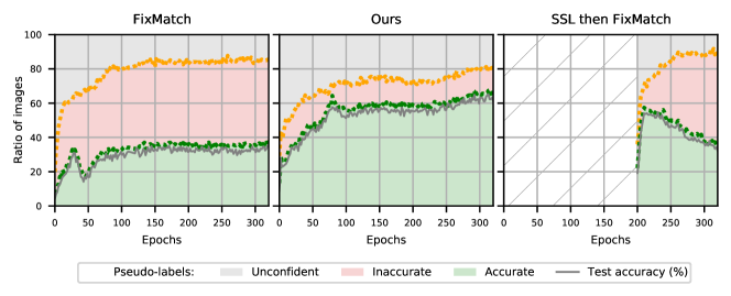
Figure 3: Evolution of the pseudo-labels during training. For each method (FixMatch, our composite loss, and SSL-then-FixMatch from left to right), we show the ratio of images with correct and confident pseudo-labels (bottom green area), incorrect but confident pseudo-labels (red area) and unconfident pseudo-labels (grey area). We also plot the test accuracy with a black line. For SSL-then-FixMatch, early training corresponds to self-supervised learning, thus these information are not available.

We present the datasets and experimental setup in Section 5.1 and validate our general idea on STL-10 in Section 5.2. We then ablate the improvements for the pseudo-label accuracy in Section 5.3, add evaluations on CIFAR in Section 5.4 and compare to the state of the art in Section 5.5.

5.1 Experimental setup

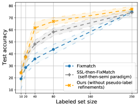
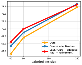
	STL-10
	$40$ labels	$80$ labels	$250$ labels
Fixmatch	$35.8$ $\pm 4.5$	$43.7$ $\pm 4.1$	$74.9$ 1.2
SSL-then-FixMatch	$48.1$ $\pm 3.2$	$58.2$ $\pm 2.1$	$74.3$ $\pm 2.8$
Ours (no adaptive $\tau$ & no refinement)	$61.6$ $\pm 5.0$	$67.0$ $\pm 3.1$	$77.2$ $\pm 2.2$
Ours (no refinement)	$64.2$ $\pm 5.1$	$68.7$ $\pm 3.0$	$\bf{78.3}$ $\pm 2.3$
LESS  (Ours + adaptive $\tau$ + refinement)	$\bf{65.6}$ $\pm 5.0$	$\bf{69.9}$ $\pm 3.1$	$78.1$ $\pm 2.2$

(a)                                             (b)                                                 (c)

Figure 4: (a) Classification accuracy on STL-10 for various sizes of labeled sets; standard deviations represented with light colors. Substantial gains are observed compared to FixMatch and the self-then-semi paradigm. (b) Results on STL-10 for various sizes of labeled set, with our two improvements to refine pseudo-labels. (c) summary of our main results on STL-10.

We perform most ablations on STL-10 and also compare approaches on CIFAR-10 and CIFAR-100. We rely on a wide-ResNet WR-28-2 (Zagoruyko and Komodakis 2016) for CIFAR-10, WR-28-8 for CIFAR-100 and WR-37-2 for STL-10 and follow FixMatch for data augmentations.

The STL-10 dataset consists of $5$k labeled images of resolution $96\times 96$ split into $10$ classes, and $100$k unlabeled images. It contains images with significantly more variety and detail than images in the CIFAR datasets; it is extracted from ImageNet and unlabeled images can be very different from those in the labeled set. It remains manageable in terms of size, with twice as many images as in CIFAR-10, offering an interesting trade-off between challenge and computational resources required. We use various amounts of labeled data: $10$ ($1$ image per class), $20$, $40$, $80$, $250$, $1000$.

Metric. We report top-1 accuracy for all datasets. In barely-supervised learning, the choice of the few labeled images can have a large impact on the final accuracy, so we report means and standard deviations over multiple runs. Standard deviations increase as the number of labels decreases, so we average across $4$ random seeds for $4$ images per class or less, $3$ otherwise, and across the last $10$ checkpoints of all runs.

5.2 Validating our composite approach on STL-10

To validate our approach, we train the baselines and our models with progressively smaller sets of labeled images; the goal is to reach a performance that degrades gracefully when progressively going to the barely-supervised regime.

To demonstrate the benefit of our composite loss from Equation 7 (without the proposed pseudo-label quality improvements of Section 4.2), we first compare this to the original FixMatch loss in Figure 4 (c) on the STL-10 dataset when training with different sizes of labeled sets, namely $\{10,20,40,80,250\}$ labeled images. We use $\tau=0.95$ for FixMatch and $\tau=0.98$ for our model, see Section 5.3 for discussions about setting $\tau$. Our approach (yellow curve) significantly outperforms FixMatch (blue curve), especially in the regime with $40$ or $80$ labeled images where the test accuracy improves by more than $20\%$. When more labeled images are considered (e.g. $250$), the gain is smaller. When only $1$ image per class is labeled, the difference is also small but our approach remains the most label efficient.

We also compare to a method using a self-then-semi paradigm, where online deep-clustering is first used alone before FixMatch is run on top of this pretrained model (grey curve labeled Self-then-FixMatch). While it performs better than FixMatch applied from scratch, we also outperform this approach, in particular in barely-supervised scenario, i.e., with less than 10 images per class.

To better analyze these results, we show in Figure 3 the evolution of pseudo-label quality for our approach, FixMatch and SSL-then-FixMatch. Our method has less examples with confident pseudo-labels in the early training; we can set a higher value of $\tau$, as we do not suffer from signal scarcity in case of unconfident pseudo-labels. In contrast, FixMatch assigns more confident pseudo-labels in early training, at the expense of a higher number of erroneous pseudo-labels, leading eventually to more errors due to error drift, also named confirmation bias. Note that the test accuracy is highly correlated to the ratio of training images with correct pseudo-labels, and thus error drift harms final performance. When comparing SSL-then-FixMatch to FixMatch, we observe that the network is quickly able to learn confident predictions, with a lesser ratio of incorrect pseudo-labels. However this ratio is still higher than with our approach. When evaluating pre-trained models, we use model checkpoints obtained between $10$ and $20$ epochs, because more training harms the performance due to confirmation bias. This was cross-validated on a single run using $80$ labeled images, and used for all other seeds and labeled sets.

5.3 Improving pseudo-label accuracy

We now evaluate the modifications proposed in Section 4.2, as well as the impact of $\tau$ to further improve performance.

Impact of the confidence threshold. The simplest way to trade-off quality and the amount of pseudo-labels, both for FixMatch and our method, is to change the confidence threshold. In Table 1, we train both methods for values of $\tau$ in $\{0.95,0.98,0.995\}$, with labeled-split sizes in $\{40,80\}$. The first finding is that the average performance of FixMatch degrades when increasing $\tau$; in particular, with $40$ labeled images, it drops by $1.9\%$ (resp. $7.4\%$) when increasing $\tau$ from $0.95$ to $0.98$ (resp. $0.995.$) Thus the default value of $\tau=0.95$ used in (Sohn et al. 2020), is the best choice; the improved pseudo-label quality obtained from increasing $\tau$ is counterbalanced by signal scarcity, see Section 3.2.

On the other hand, the performance of our method improves when increasing $\tau$; in particular, with $40$ labeled images, it increases by $2.4\%$. As expected, our method benefits from using self-supervised training signal in the absence of confident pseudo-labels, which allows us to raise $\tau$ without signal scarcity, and without degrading the final accuracy. The performance of our method remains stable when raising $\tau$ to $0.995$; this demonstrates that it is robust to high threshold values, even though this does not bring further accuracy improvements. For the rest of the experiments we keep $\tau=0.98$ for our method and $\tau=0.95$ for FixMatch.

$\tau$	FixMatch		Ours (w/o refinements)
	40 labels	80 labels	40 labels	80 labels
0.95	$\bf{35.8}$ $\pm 4.5$	$\bf{48.1}$ $\pm 3.2$	$61.8$ $\pm 4.9$	$67.2$ $\pm 2.9$
0.98	$33.9$ $\pm 4.7$	$47.4$ $\pm 3.5$	$\bf{64.2}$ $\pm 5.1$	$\bf{68.7}$ $\pm 3.0$
0.995	$28.4$ $\pm 6.2$	$46.3$ $\pm 3.7$	$64.1$ $\pm 4.3$	$68.6$ $\pm 2.8$

Table 1: Ablation on the threshold parameter $\tau$ on the STL-10 dataset for $40$ and $80$ labeled images. The default value of $0.95$ works best for FixMatch. Our method benefits from increasing $\tau$ to $0.98$, and is more robust to a higher threshold value of $0.995$.

Adaptive threshold and confidence refinement. We now validate the usefulness of the class-aware confident threshold presented in Section 4.2. We plot in Figure 4 (b) the performance of our model, with (blue line) and without it (yellow line). Adaptive thresholds demonstrate consistent gains across labeled-set sizes, e.g. with an average gain of $2.6\%$ when using $40$ labels. This validates the approach of bolstering the exploration of classes that are under represented in the model predictions, while focusing on the most confident labels for classes that are well represented. The gains observed are more substantial for low numbers of labeled images, like $40$ compared to $250$, which suggests that when using a fixed threshold, exploration may naturally be more balanced with more labeled images.

Impact of using pseudo-label refinement on our method. We now evaluate the refinement of pseudo-labels using a set of predictions for different augmentations $u\in\mathcal{A}$, see Section 4.2. Figure 4(b) reports performance for models trained with Equation 7, with (red curve) and without refined labels (blue curve). Using the refined labels offers a $1.4\%$ (resp. $1.1\%$) accuracy improvement on average when using $40$ (resp. $80$) labels, on top of the gains already obtained from using our composite loss, and adaptive thresholds. No improvement is observed, however, with 250 labels.

5.4 Comparison on CIFAR

	CIFAR-10			CIFAR-100
	$10$ labels	$40$ labels	$250$ labels	$100$ labels	$200$ labels	$400$ labels
FixMatch	$56.1$ $\pm 11.3$	$92.1$ $\pm 3.4$	$94.0$ $\pm 0.9$	$23.1$ $\pm 4.7$	$38.6$ $\pm 3.5$	$50.2$ $\pm 2.1$
LESS	$\bf{64.4}$ $\pm 10.9$	$\bf{93.2}$ $\pm 2.1$	$\bf{95.0}$ $\pm 0.8$	$\bf{28.2}$ $\pm 3.0$	$\bf{42.5}$ $\pm 3.2$	$\bf{51.3}$ $\pm 2.4$

Table 2: Comparison of our approach and FixMatch for barely-supervised learning on CIFAR-100 and CIFAR-10. All results obtained using the same code base. As labels becomes more scarce, greater performance gains are observed with our method.

So far, we drew the comparison on STL-10 dataset only. We now compare our method with pseudo-labels quality improvements, denoted as LESS for Label-Efficient Semi-Supervised learning, to FixMatch on CIFAR-10 and CIFAR-100 with labeled set sizes of $1$, $2$ or $4$ samples per class in Table 2. For CIFAR-10 we report results for our model with $\tau=0.995$, as we found it to be the best among $\{0.95,0.98,0.995\}$. We observe that our approach outperforms FixMatch for all cases, with a gain ranging from $5\%$ with 1 label per class to $1\%$ with 4 labels per class on CIFAR-100, and from $8\%$ with 1 label per class to $1\%$ with 25 labels per class on CIFAR-10. The gain here is smaller than the one reported on STL-10. We hypothesize that the very low resolution ($32\times 32$) of CIFAR images leads to less powerful self-supervised training signals.

5.5 Comparison to the state of the art

We finally compare our approach to numbers reported in others papers in Table 3. Note that all previous papers reported numbers on STL-10 are with 1000 labels (i.e., 100 labels per class), which cannot be considered as barely-supervised.We thus only provide a comparison on the CIFAR-10 dataset where other methods reported results for smaller numbers of images per class. We observe that our approach performs the best on the CIFAR-10 dataset, in particular with 4 labels per class. Tthe gap with the self-then-semi paradigm is lower on this dataset as it is significantly less challenging than STL-10. Note that the previous results of FixMatch in Table 2 were obtained with our code-base, which explains the slightly different performance compared to the numbers in Table 3.

	CIFAR-10
	40 labels	250 labels
Semi-supervised from scratch
Pseudo-Label (Lee 2013)	-	$50.2$ $\pm 0.4$
$\Pi$-Model (Rasmus et al. 2015)	-	$45.7$$\pm 3.9$
Mean Teacher (Tarvainen and Valpola 2017)	-	$67.7$$\pm 2.3$
MixMatch (Berthelot et al. 2019b)	$52.5$ $\pm 11.5$	$89.0$ $\pm 0.9$
UDA (Xie et al. 2019)	$71.0$ $\pm 5.9$	$91.2$ $\pm 1.1$
ReMixMatch (Berthelot et al. 2019a)	$80.9$ $\pm 9.6$	$94.6$ $\pm 0.1$
FixMatch (Sohn et al. 2020) (with RA (Cubuk et al. 2020))	$86.1$ $\pm 3.4$	$94.9$ $\pm 0.7$
Self-then-semi paradigm
SelfMatch (Kim et al. 2020)	$\bf{93.2}$ $\pm 1.1$	$\bf{95.1}$ $\pm 0.3$
CoMatch (Li, Xiong, and Hoi 2021)	$93.1$$\pm 1.4$	$\bf{95.1}$ $\pm 0.3$
Composite self- and semi-supervised
LESS	$\bf{93.2}$ $\pm 2.1$	$\bf{95.1}$ $\pm 0.8$
Fully-Supervised	95.9

Table 3: Comparison to state-of-the-art methods on CIFAR.

6 Conclusion

After analyzing the behavior of FixMatch in the barely-supervised learning scenario, we found that one critical limitation was due to the distillation dilemma. We proposed to leverage self-supervised training signals when no confident pseudo-label were predicted and showed that this composite approach allows to significantly increase performance. We additionally proposed two refinement strategies to improve pseudo-label quality during training and further increase test accuracy. Further research directions include extension to datasets with more classes such as ImageNet. Other related topics such as model calibration and learning with noisy labels are also directions that we expect to be critical to progress in barely-supervised learning.

References

- Arazo et al. (2020) Arazo, E.; Ortego, D.; Albert, P.; O’Connor, N. E.; and McGuinness, K. 2020. Pseudo-labeling and confirmation bias in deep semi-supervised learning. In IJCNN.
- Asano, Rupprecht, and Vedaldi (2020) Asano, Y. M.; Rupprecht, C.; and Vedaldi, A. 2020. A critical analysis of self-supervision, or what we can learn from a single image. In ICLR.
- Bachman, Alsharif, and Precup (2014) Bachman, P.; Alsharif, O.; and Precup, D. 2014. Learning with pseudo-ensembles. In NIPS.
- Berthelot et al. (2019a) Berthelot, D.; Carlini, N.; Cubuk, E. D.; Kurakin, A.; Sohn, K.; Zhang, H.; and Raffel, C. 2019a. ReMixMatch: Semi-supervised learning with distribution alignment and augmentation anchoring. In ICLR.
- Berthelot et al. (2019b) Berthelot, D.; Carlini, N.; Goodfellow, I. J.; Papernot, N.; Oliver, A.; and Raffel, C. 2019b. MixMatch: A Holistic Approach to Semi-Supervised Learning. In NeurIPS.
- Cai et al. (2021) Cai, Z.; Ravichandran, A.; Maji, S.; Fowlkes, C.; Tu, Z.; and Soatto, S. 2021. Exponential Moving Average Normalization for Self-supervised and Semi-supervised Learning. CVPR.
- Caron et al. (2020) Caron, M.; Misra, I.; Mairal, J.; Goyal, P.; Bojanowski, P.; and Joulin, A. 2020. Unsupervised Learning of Visual Features by Contrasting Cluster Assignments. In NeurIPS.
- Chen et al. (2020a) Chen, T.; Kornblith, S.; Norouzi, M.; and Hinton, G. 2020a. A simple framework for contrastive learning of visual representations. In ICML.
- Chen et al. (2020b) Chen, T.; Kornblith, S.; Swersky, K.; Norouzi, M.; and Hinton, G. 2020b. Big self-supervised models are strong semi-supervised learners. In NeurIPS.
- Chen et al. (2020c) Chen, X.; Fan, H.; Girshick, R.; and He, K. 2020c. Improved baselines with momentum contrastive learning. arXiv preprint arXiv:2003.04297.
- Chen and He (2021) Chen, X.; and He, K. 2021. Exploring Simple Siamese Representation Learning.
- Cubuk et al. (2020) Cubuk, E. D.; Zoph, B.; Shlens, J.; and Le, Q. V. 2020. RandAugment: Practical data augmentation with no separate search.
- Doersch, Gupta, and Efros (2015) Doersch, C.; Gupta, A.; and Efros, A. A. 2015. Unsupervised visual representation learning by context prediction. In ICCV.
- Dosovitskiy et al. (2014) Dosovitskiy, A.; Springenberg, J. T.; Riedmiller, M.; and Brox, T. 2014. Discriminative unsupervised feature learning with convolutional neural networks. In NIPS.
- Gidaris, Singh, and Komodakis (2018) Gidaris, S.; Singh, P.; and Komodakis, N. 2018. Unsupervised representation learning by predicting image rotations. In ICLR.
- Gontijo-Lopes et al. (2020) Gontijo-Lopes, R.; Smullin, S. J.; Cubuk, E. D.; and Dyer, E. 2020. Affinity and diversity: Quantifying mechanisms of data augmentation. arXiv preprint arXiv:2002.08973.
- Grill et al. (2020) Grill, J.-B.; Strub, F.; Altché, F.; Tallec, C.; Richemond, P. H.; Buchatskaya, E.; Doersch, C.; Pires, B. A.; Guo, Z. D.; Azar, M. G.; et al. 2020. Bootstrap your own latent: A new approach to self-supervised learning. In NeurIPS.
- Guo et al. (2017) Guo, C.; Pleiss, G.; Sun, Y.; and Weinberger, K. Q. 2017. On Calibration of Modern Neural Networks. PMLR.
- Han et al. (2021) Han, T.; Gao, J.; Yuan, Y.; and Wang, Q. 2021. Unsupervised Semantic Aggregation and Deformable Template Matching for Semi-Supervised Learning. NeurIPS.
- He et al. (2020) He, K.; Fan, H.; Wu, Y.; Xie, S.; and Girshick, R. 2020. Momentum contrast for unsupervised visual representation learning. In CVPR.
- He et al. (2016) He, K.; Zhang, X.; Ren, S.; and Sun, J. 2016. Deep residual learning for image recognition. In CVPR.
- Hu, Yang, and Nevatia (2021) Hu, Z.; Yang, Z.; and Nevatia, X. H. R. 2021. SimPLE: Similar Pseudo Label Exploitation for Semi-Supervised Classification. CVPR.
- Javanovic and Levy (1997) Javanovic; and Levy. 1997. A look at the rule of Three. Journal of the American Statistician.
- Kim et al. (2020) Kim, B.; Choo, J.; Kwon, Y.-D.; Joe, S.; Min, S.; and Gwon, Y. 2020. SelfMatch: Combining Contrastive Self-Supervision and Consistency for Semi-Supervised Learning. In NeurIPS workshop.
- Krizhevsky, Sutskever, and Hinton (2012) Krizhevsky, A.; Sutskever, I.; and Hinton, G. E. 2012. Imagenet classification with deep convolutional neural networks. In NIPS.
- Lee (2013) Lee, D.-H. 2013. Pseudo-label: The simple and efficient semi-supervised learning method for deep neural networks. In ICML workshop.
- Lerner, Shiran, and Weinshall (2020) Lerner, B.; Shiran, G.; and Weinshall, D. 2020. Boosting the Performance of Semi-Supervised Learning with Unsupervised Clustering. arXiv.
- Li, Xiong, and Hoi (2021) Li, J.; Xiong, C.; and Hoi, S. 2021. CoMatch: Semi-supervised Learning with Contrastive Graph Regularization.
- Li et al. (2020) Li, S.; Liu, B.; Chen, D.; Chu, Q.; Yuan, L.; and Yu, N. 2020. Density-Aware Graph for Deep Semi-Supervised Visual Recognition. CVPR.
- Neumann, Zisserman, and Vedaldi (2018) Neumann, L.; Zisserman, A.; and Vedaldi, A. 2018. Relaxed Softmax: Efficient Confidence Auto-Calibration for Safe Pedestrian Detection. In NeurIPS Workshop.
- Nixon et al. (2019) Nixon, J.; Dusenberry, M.; Zhang, L.; Jerfel, G.; and Tran, D. 2019. Measuring Calibration in Deep Learning. In CVPR.
- Noroozi and Favaro (2016) Noroozi, M.; and Favaro, P. 2016. Unsupervised learning of visual representations by solving jigsaw puzzles. In ECCV.
- Pham et al. (2021) Pham, H.; Dai, Z.; Xie, Q.; Luong, M.-T.; and Le, Q. V. 2021. Meta Pseudo Labels.
- Purushwalkam and Gupta (2020) Purushwalkam, S.; and Gupta, A. 2020. Demystifying contrastive self-supervised learning: Invariances, augmentations and dataset biases. In NeurIPS.
- Rasmus et al. (2015) Rasmus, A.; Valpola, H.; Honkala, M.; Berglund, M.; and Raiko, T. 2015. Semi-supervised learning with ladder networks. In NIPS.
- Rosenberg, Hebert, and Schneiderman (2005) Rosenberg, C.; Hebert, M.; and Schneiderman, H. 2005. Semi-supervised self-training of object detection models. In WACV.
- Sajjadi, Javanmardi, and Tasdizen (2016) Sajjadi, M.; Javanmardi, M.; and Tasdizen, T. 2016. Regularization with stochastic transformations and perturbations for deep semi-supervised learning. In NIPS.
- Simonyan and Zisserman (2015) Simonyan, K.; and Zisserman, A. 2015. Very deep convolutional networks for large-scale image recognition. In ICLR.
- Sohn et al. (2020) Sohn, K.; Berthelot, D.; Li, C.-L.; Zhang, Z.; Carlini, N.; Cubuk, E. D.; Kurakin, A.; Zhang, H.; and Raffel, C. 2020. FixMatch: Simplifying Semi-Supervised Learning with Consistency and Confidence. In NeurIPS.
- Tarvainen and Valpola (2017) Tarvainen, A.; and Valpola, H. 2017. Mean teachers are better role models: Weight-averaged consistency targets improve semi-supervised deep learning results. In NeurIPS.
- Tian et al. (2020) Tian, Y.; Sun, C.; Poole, B.; Krishnan, D.; Schmid, C.; and Isola, P. 2020. What makes for good views for contrastive learning. In NeurIPS.
- Wu et al. (2018a) Wu, Z.; Xiong, Y.; Yu, S. X.; and Lin, D. 2018a. Unsupervised feature learning via non-parametric instance discrimination. In CVPR.
- Wu et al. (2018b) Wu, Z.; Xiong, Y.; Yu, S. X.; and Lin, D. 2018b. Unsupervised feature learning via non-parametric instance discrimination. In CVPR.
- Xie et al. (2019) Xie, Q.; Dai, Z.; Hovy, E.; Luong, M.-T.; and Le, Q. V. 2019. Unsupervised data augmentation for consistency training. In NeurIPS.
- Xie et al. (2020) Xie, Q.; Luong, M.-T.; Hovy, E.; and Le, Q. V. 2020. Self-training with noisy student improves imagenet classification. In CVPR.
- Yarowsky (1995) Yarowsky, D. 1995. Unsupervised word sense disambiguation rivaling supervised methods. In 33rd annual meeting of the association for computational linguistics.
- Zagoruyko and Komodakis (2016) Zagoruyko, S.; and Komodakis, N. 2016. Wide Residual Networks. In BMVC.
- Zhai et al. (2019) Zhai, X.; Oliver, A.; Kolesnikov, A.; and Beyer, L. 2019. S4L: Self-supervised semi-supervised learning. In ICCV.
- Zhang and Sabuncu (2020) Zhang, Z.; and Sabuncu, M. R. 2020. Self-Distillation as Instance-Specific Label Smoothing. In NeurIPS.