Nonlinear transverse current on $\mathcal{C}_{3v}$-symmetric honeycomb lattice

Abstract

At nonlinear orders in the electric field, the vanishing of the Hall conductivity does not prevent the nonlinear component of the current from being transverse for selected field directions. We study electrons on $\mathcal{C}_{3v}$-symmetric honeycomb lattice for which the Hall conductivity vanishes at first and second order. Nevertheless, the second-order current component is transverse for fields perpendicular to the three mirror lines. The $\mathcal{C}_{3v}$ symmetry constrains the first-order and second-order conductivity tensors to have only one independent component each, which we calculate using the quantum kinetic equation. In linearly-polarized oscillating field, the current has a zero-frequency component switching sign upon $\pi/2$-rotation of the polarization angle.

The description of the quantum Hall effect in terms of the electronic Berry phase is a milestone of modern solid state physics [1]. At linear order in the applied field, the Hall conductivity is related to the Berry curvature and vanishes by time-reversal symmetry [2]. At second order, it is induced by the Berry-curvature dipole and can be finite also in time-reversal-invariant systems, provided a low crystal symmetry [3]. Specifically, it requires broken inversion symmetry and at most one mirror symmetry and has been indeed detected in layered transition-metal dichalcogenides with one mirror plane [4, 5].

In this work we consider electrons on the honeycomb lattice with a site-potential imbalance, whose symmetry point group $\mathcal{C}_{3v}$ features a $2\pi/3$-rotation axis and three mirror lines. Since the system has also time-reversal symmetry, the Hall conductivity vanishes at first and second order. Nevertheless, the second-order current component is reminiscent of a Hall current, since it is transverse for fields perpendicular to the mirror lines. Within the quantum-kinetic framework, we numerically calculate the conductivity tensor up to second order and discuss its dependence on site-potential imbalance and relaxation time. Finally, we calculate the response to linearly-polarized oscillating field and its zero-frequency component, which originates from the second-order response and switches sign upon $\pi/2$-rotation of the polarization angle.

I Nonlinear transverse current in systems with vanishing Hall conductivity

Let us start by illustrating in simple terms the unique property of nonlinear current responses, namely they can be transverse, meaning perpendicular to the applied field, even with vanishing Hall conductivity. Let us consider a two-dimensional system and assume the electric-current density $j_{\alpha}$ ($\alpha=x,y$) admits a power-series expansion in the electric field $E_{\alpha}$, which up to second order reads

$$j_{\alpha}=\sigma_{\alpha\beta}E_{\beta}+\chi_{\alpha\beta\gamma}E_{\beta}E_{\gamma}.$$ (1)

The Hall conductivity at each order is the antisymmetric part of the conductivity, $\epsilon_{\alpha\beta}\epsilon_{\zeta\eta}\sigma_{\zeta\eta}$ and $\epsilon_{\alpha\beta}\epsilon_{\zeta\eta}\chi_{\zeta\eta\gamma}$, hence the symmetry constraints on the Hall effect [6, 7, 8]. The Hall current is therefore by definition transverse and dissipationless, namely it does not contribute to the power

$$j_{\alpha}E_{\alpha}=\sigma_{\alpha\beta}E_{\alpha}E_{\beta}+\chi_{\alpha\beta\gamma}E_{\alpha}E_{\beta}E_{\gamma}.$$ (2)

The two terms on the right-hand-side of Eq. (2) have a remarkable difference: the first is a quadratic form and vanishes if and only if $\sigma_{\alpha\beta}$ is antisymmetric; the second is a cubic form and the antisymmetry of $\chi_{\alpha\beta\gamma}$ in $\alpha$ and $\beta$ is sufficient but not necessary for it to vanish. Indeed, there is in general at least one field direction which makes the second term on the right-hand-side of Eq. (2) to vanish, meaning that the second-order component in Eq. (1) is transverse [9]. In other words, at (and only at) nonlinear orders in the applied electric field, the nonlinear component of the current is transverse for selected field directions, no matter the vanishing of the Hall effect.

II Second-order current in $\mathcal{C}_{3v}$-symmetric systems

We now turn to the case of $\mathcal{C}_{3v}$ symmetry, which applies to the honeycomb lattice with site-potential imbalance, see Fig. 1. To derive the symmetry constraints, we fix a choice of coordinate axes – $\hat{x}$ parallel to one of the mirror lines – and impose the symmetries $\sigma_{v}^{\prime}$ and $C_{3}$, namely the reflection with respect to the $x$ axis and the $2\pi/3$-rotation. The resulting constraints read [10]

$$\begin{aligned} \sigma_{xy}=\sigma_{yx}&=0,\\ \sigma_{xx}=\sigma_{yy}&\equiv\sigma,\end{aligned}$$

$$\begin{aligned} \chi_{xxy}=\chi_{xyx}=\chi_{yxx}=\chi_{yyy}&=0,\\ -\chi_{xxx}=\chi_{xyy}=\chi_{yxy}=\chi_{yyx}&\equiv-\chi.\end{aligned}$$

Thus the entire response up to second order depends only on two coefficients $\sigma$ and $\chi$ (not to be confused with the tensors $\sigma_{\alpha\beta}$, $\chi_{\alpha\beta\gamma}$). In particular, Eq. (3) states that the second-order non-diagonal components with odd number of “$x$-indices” are equal to each other but need not be vanishing. The latter fact relates to the broken $x$-axis-reversal symmetry (reflection with respect to the $y$ axis) by the site-potential imbalance, see Fig. 1. The meaning of $\chi_{xyy}$ is particularly clear as it gives a response along $\hat{x}$ to a field along $\hat{y}$. Note that the Hall conductivity vanishes at first ($\epsilon_{\alpha\beta}\sigma_{\alpha\beta}=0$) and second order ($\epsilon_{\alpha\beta}\chi_{\alpha\beta\gamma}=0$) consistently with well known symmetry constraints [6].

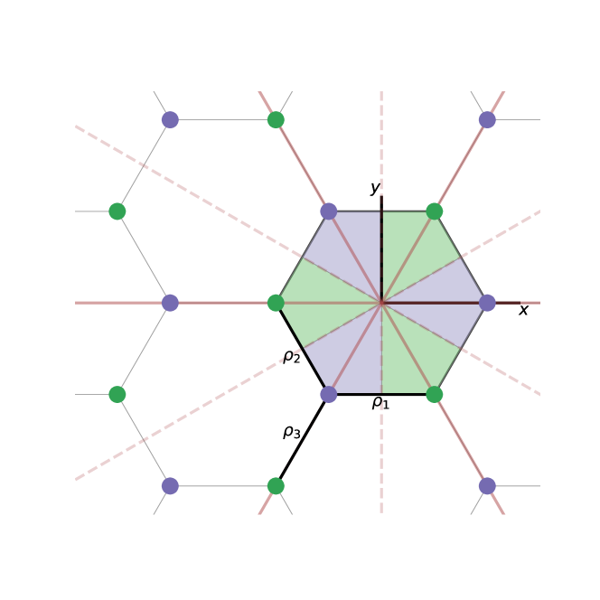
Figure 1: $\mathcal{C}_{3v}$-symmetric honeycomb lattice. Sites on sublattice $A$ (blue) and $B$ (green) have potential imbalance $\pm m$. The symmetry point group (with respect to, e.g., the center of each hexagon) include rotations of $2\pi/3$ and $4\pi/3$ and three reflections (with respect to the solid orange lines). For $m=0$ appear three additional mirror lines (dashed orange lines).

Plugging Eqs. (3) into Eq. (1) yields the current up to second order in the field $\bm{E}=(E_{x},E_{y})=E(\cos\theta,\sin\theta)$ of a system with $\mathcal{C}_{3v}$ symmetry:

$$j_{x} =\sigma E_{x}+\chi(E_{x}^{2}-E_{y}^{2}),$$ (4a)

$$j_{y} =\sigma E_{y}-2\chi E_{x}E_{y}.$$ (4b)

The second-order component forms an angle $-2\theta$ with $\hat{x}$, hence it is transverse for $\theta=\pi/6+n\pi/3$ and longitudinal for $\theta=n\pi/3$ ($n$ integer). In other words, it is transverse or longitudinal for fields perpendicular or parallel to the three mirror lines, which on honeycomb lattice coincide with the three bond directions $\hat{\bm{\rho}}_{n}=(\cos\phi_{n},\sin\phi_{n})$ with $\phi_{n}=2\pi n/3$ ($n=1,2,3)$, see Fig. 1.

Equations (4) can be written in the invariant fashion which does not depend on the choice of coordinate axes and makes the $\mathcal{C}_{3v}$ symmetry manifest together with the direction of the second-order current:

$$\bm{j}=\sigma\bm{E}+(4/3)\chi\sum_{(i,j,k)\in P_{3}}(\bm{E}\cdot\hat{\bm{\rho}}_{i})(\bm{E}\cdot\hat{\bm{\rho}}_{j})\hat{\bm{\rho}}_{k},$$ (5)

where $P_{3}=\{(1,2,3),(2,3,1),(3,1,2)\}$. Furthermore, we can express the conductivity tensors as $\sigma_{\alpha\beta}=\sigma\delta_{\alpha\beta}$ and $\chi_{\alpha\beta\gamma}=(4/3)\chi\ \sum_{(i,j,k)\in P_{3}}\hat{\rho}_{i\alpha}\hat{\rho}_{j\beta}\hat{\rho}_{k\gamma}$ which make evident the symmetry of these tensors, hence the vanishing of the Hall effect. The dissipated power reads

$$\bm{j}\cdot\bm{E}=\sigma|\bm{E}|^{2}+4\chi(\bm{E}\cdot\hat{\bm{\rho}}_{1})(\bm{E}\cdot\hat{\bm{\rho}}_{2})(\bm{E}\cdot\hat{\bm{\rho}}_{3}),$$ (6)

and it is clear that the second-order current component is dissipationless for fields perpendicular to the three bonds.

III Model and methods

To proceed with the calculation of conductivity tensors and nonlinear transverse current, we consider the tight-binding Hamiltonian on honeycomb lattice [11]

$$H=\sum\nolimits_{\bm{k}}\Psi_{\bm{k}}^{\dagger}H_{\bm{k}}\Psi_{\bm{k}},$$ (7)

$$H_{\bm{k}}=(\text{Re}f_{\bm{k}})t_{h}\sigma_{1}+(\text{Im}f_{\bm{k}})t_{h}\sigma_{2}+m\sigma_{3},$$ (8)

$$f_{k}=\exp(i{\bm{k}}\cdot{\bm{\rho}}_{1})+\exp(i{\bm{k}}\cdot{\bm{\rho}}_{2})+\exp(i{\bm{k}}\cdot{\bm{\rho}}_{3}).$$ (9)

Here $\Psi_{\bm{k}}=(c_{{\bm{k}}A},c_{{\bm{k}}B})^{T}$ where $c_{{\bm{k}}A(B)}$ is the lattice Fourier transform of the electronic annihilation operator on the sublattice $A(B)$, $\sigma_{i}$ ($i=1,2,3$) are Pauli matrices, $t_{h}$ is the nearest-neighbor hopping, $m$ is the site-potential imbalance and $\bm{\rho}_{n}=a\hat{\bm{\rho}}_{n}$ with $a$ nearest-neighbor distance.

The density matrix $\rho_{\bm{k}}^{ab}=\braket{\Psi_{\bm{k}}^{b\dagger}\Psi_{\bm{k}}^{a}}$ ($a,b=1,2$) evolves in time according to the quantum kinetic equation

$$\dot{\rho}_{\bm{k}}=i\hbar^{-1}[\rho_{\bm{k}},H_{{\bm{k}}+e\bm{A}(t)/\hbar}]-\tau^{-1}(\rho_{\bm{k}}-\rho_{{\bm{k}}+e\bm{A}(t)/\hbar}^{0}).$$ (10)

The first term on the right-hand side of Eq. (10) gives the unitary evolution with Hamiltonian with shifted crystal momentum, where $\bm{A}(t)=-\bm{E}t$ is the gauge field and $\bm{E}$ the electric field. The second term provides dissipation with relaxation time $\tau$, $\rho_{\bm{k}}^{0}=[1+\exp(H_{\bm{k}}/k_{B}T)]^{-1}$ is the equilibrium density matrix at a temperature $T=0$. The current density is $\bm{j}=(2\pi^{2})^{-1}\int\text{d}^{2}{\bm{k}}\text{Tr}(\rho_{\bm{k}}e\bm{v}_{{\bm{k}}+e\bm{A}(t)/\hbar})$ where $\bm{v}_{\bm{k}}=\hbar^{-1}\nabla_{\bm{k}}H_{\bm{k}}$, the integral is over the Brillouin zone and both spin directions are taken into account.

The system is a band insulator with gap $\Delta_{g}=2m$ for $m\neq 0$ and a semimetal for $m=0$. Equation (1) is typically used only for metallic systems, see e. g. Ref. [6]. To use it also for $m\neq 0$ is acceptable for a certain range of $\tau$ and $E$, as we discuss again below and as ultimately confirmed by the numerical integration of Eq. (10) in Sec. IV.

The quantum kinetic equation with relaxation-time approximation, Eq. (10), has been recently used in similar setups, for instance to study the light-induced anomalous Hall effect in graphene [12], see also Refs. [13, 14], and the electron-hole pair creation in rotating electric fields [15].

IV First-order and second-order conductivity coefficients

We present here the numerical calculation of the time evolution in static electric field and, from the steady-state current, we extract the first-order $\sigma$ and second-order $\chi$ conductivity coefficients, discussing the dependence on site-potential imbalance $m$ and relaxation time $\tau$.

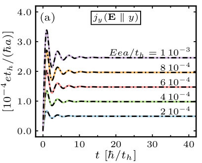
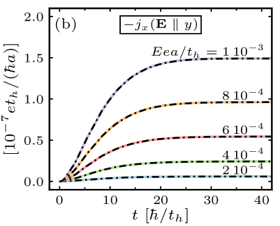
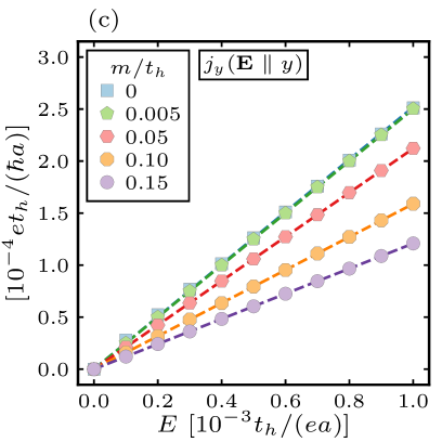
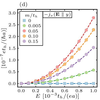
Figure 2: Top panels: Time evolution of (solid) (a) longitudinal current $j_{y}(\bm{E}\parallel\hat{y})$ and (b) transverse current $j_{x}(\bm{E}\parallel\hat{y})$; with (dash-dotted) symmetrized longitudinal current $j_{x}(\bm{E}\parallel\hat{x})$ according to Eqs. (11); $m/t_{h}=0.015$, $\tau t_{h}/\hbar=5$. Bottom panels: Steady-state (markers) (c) longitudinal current $j_{y}(\bm{E}\parallel\hat{y})$ and (d) transverse current $j_{x}(\bm{E}\parallel\hat{y})$; with (dashed) respectively linear and quadratic fits; $\tau t_{h}/\hbar=5$.

In Fig. 2(a),(b) we plot the time evolution of $j_{y}(\bm{E}\parallel\hat{y})$ and $j_{x}(\bm{E}\parallel\hat{y})$, longitudinal and transverse components of the current. In agreement with our expectations based on Eqs. (4), for $m\neq 0$ and field along $\hat{y}$ (perpendicular to a mirror line) the system sustains a transverse current invariant upon field reversal ($\bm{E}\rightarrow-\bm{E}$), as we have also checked (not shown). To further substantiate Eqs. (4), we derive opportune combinations of longitudinal currents $j_{x}(\bm{E}\parallel\pm\hat{x})$ in fields of the same amplitude along $\pm\hat{x}$, which relate to the current in field along $\hat{y}$ as

$$\frac{j_{x}(E,0)-j_{x}(-E,0)}{2} =j_{y}(0,E),$$ (11a)

$$\frac{j_{x}(E,0)+j_{x}(-E,0)}{2} =-j_{x}(0,E).$$ (11b)

The left-hand-side of Eqs. (11), derived from Eqs. (4), is also plotted in Fig. 2(a),(b) (dash-dotted), supporting the validity of the power-series expansion Eq. (1) and of the consequent Eqs. (4) in this range of parameters.

The steady-state current versus the field amplitude is plotted in Fig. 2(c),(d). Longitudinal and transverse currents are linear and quadratic, respectively. At fixed $E$, the former decreases with $m$, while the latter vanishes for $m=0$, then increases with $m$ and finally also decreases.

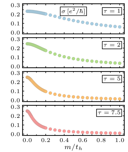
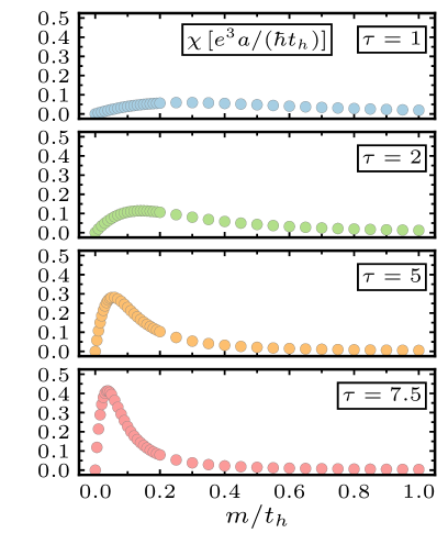
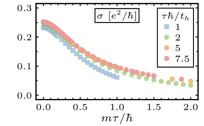
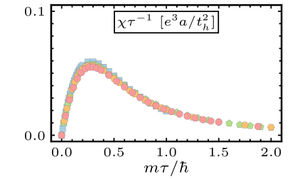
Figure 3: Top panels: First-order (left) and second-order (right) conductivity coefficients $\sigma$, $\chi$ versus site-potential imbalance $m/t_{h}$ and for varying relaxation time $\tau$. $\sigma$ is monotonous decreasing to zero at large $m$, $\chi$ vanishes at $m=0$, is maximum at $m^{*}$, and finally goes to zero at large $m$. Bottom panels: curve collapse with $\sigma\rightarrow\sigma$, $\chi\rightarrow\chi\tau^{-1}$, $m\rightarrow m\tau$ showing the scaling relations $\sigma(m=0)\sim\tau^{0}$, $\chi(m=m^{*})\sim\tau^{1}$, $m^{*}\sim\tau^{-1}$.

To extract the coefficients $\sigma$ and $\chi$, we fit longitudinal and transverse steady-state currents as $j_{y}(\bm{E}\parallel\hat{y})=\sigma E$ and $j_{x}(\bm{E}\parallel\hat{y})=-\chi E^{2}$ cf. Eqs. (4). The fitting lines are plotted in Fig. 2(c),(d) (dashed) and the coefficients in Fig. 3 (top panels) versus $m$ and for varying $\tau$.

The numerical result shows that, for each $m$, $\tau$, Eqs. (4) are valid at small enough $E$ [10]. Decreasing $m$ or $\tau$ requires smaller $E$ in order to extract $\sigma$ and $\chi$. Note that, indeed, for small $E$ and $\tau$ the density matrix expands in a double power-series [6] leading in turn to a power-series for the current. Specifically, here we use $Eea/t_{h}<0.01$ for $m/t_{h}\geq 0.25$ and/or $\tau t_{h}/\hbar=1,2$; $Eea/t_{h}<0.001$ for $m/t_{h}<0.25$ and $\tau t_{h}/\hbar=5,7.5$.

For $m=0$, $\sigma$ is maximum and $\chi$ vanishes. Indeed in this limiting case the band gap closes and three mirror lines appear, which further constrain the components of the conductivity $\chi_{\alpha\beta\gamma}$. Increasing $m$, the band gap opens and widens. Accordingly, $\sigma$ decreases while $\chi$ is instead non-monotonous: first it becomes finite as a consequence of the broken $x$-axis reversal symmetry, then reaches a maximum for $m=m^{*}$and finally also decreases. In the limit of large $m$ the band structure consists of two isolated bands – one full the other empty – and at all orders the conductivity trivially vanishes.

Increasing $\tau$ the conductivity coefficients decrease for all $m$ except for their maxima $\sigma(m=0)$ and $\chi(m=m^{*})$ which are, respectively, constant and increasing with $\tau$. Moreover, $m^{*}$ which makes $\chi$ maximum decreases with $\tau$. Guided by these observations, in Fig. 3 (bottom panels) we plot rescaled conductivity coefficients $\sigma\tau^{0}$ and $\chi\tau^{-1}$ versus rescaled site-potential $m\tau^{1}$. The curve collapse shows the validity of the approximate scaling relations $\sigma(m=0)\sim\tau^{0}$, $\chi(m=m^{*})\sim\tau^{1}$ and $m^{*}\sim\tau^{-1}$.

For $m=0$ we get $\sigma\approx 0.25\,e^{2}/\hbar$ not far from the theoretical value for two-dimensional massless Dirac electrons $4e^{2}/(\pi h)\approx 0.2\,e^{2}/\hbar$ [11]. Moreover $\chi\sim\tau^{1}$ has the same scaling as the nonlinear Hall conductivity in Refs. [3, 6].

V Zero-frequency current component in oscillating field

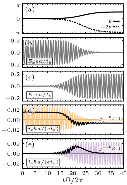
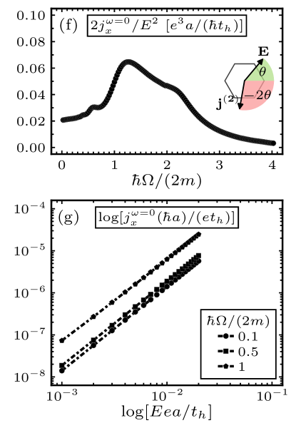
Figure 4: (a) Modulation of polarization angle of applied field $\bm{E}=E\cos(\Omega t)(\cos\theta,\sin\theta)$ and of second-order response $-2\theta$ [cf. inset panel (f)]. (b),(c) Corresponding field components. (d),(e) Time evolution of current (color) and of zero-frequency component (black); $m/t_{h}=0.5$, $\tau t_{h}/\hbar=5$, $\hbar\Omega/t_{h}=0.1$. (f) Zero-frequency component $2j_{x}^{\omega=0}/E^{2}$ with $\bm{E}ea/t_{h}=0.1\,\hat{x}$ versus field frequency $\hbar\Omega/(2m)$. (g) $j_{x}^{\omega=0}(\bm{E}\parallel\hat{x})$ versus field amplitude for varying field frequency.

Let us now consider an oscillating applied field. Since the second-order current response is invariant under field reversal [$\bm{E}\rightarrow-\bm{E}$, cf. Eqs. (4)], we expect it to have a finite time average, namely a zero-frequency component. Before presenting the numerical result, we gain insight into the response to a linearly-polarized oscillating field $\bm{E}=E\cos(\Omega t)(\cos\theta,\sin\theta)$ by substitution in Eqs. (4):

$$j_{x} =\sigma E\cos(\Omega t)\cos\theta+\chi E^{2}[\cos(\Omega t)]^{2}\cos 2\theta,$$ (12a)

$$j_{y} =\sigma E\cos(\Omega t)\sin\theta-\chi E^{2}[\cos(\Omega t)]^{2}\sin 2\theta,$$ (12b)

Since Eqs. (4) are formulated for static electric field, we expect Eqs. (12) to be approximately valid only for small frequency $\Omega$. The time average, that is the zero-frequency ($\omega=0$) current component, reads

$$j_{x}^{\omega=0} =(\chi E^{2}/2)\cos 2\theta,$$ (13a)

$$j_{y}^{\omega=0} =-(\chi E^{2}/2)\sin 2\theta.$$ (13b)

Thus indeed a zero-frequency component originates from the second-order response and forms the same angle $-2\theta$ with $\hat{x}$. Besides being transverse for $\theta=\pi/6+n\pi/3$ and longitudinal for $\theta=n\pi/3$ ($n$ integer), as discussed above, this also implies that it reverses upon $\pi/2$-rotation of the applied field, since $\theta\rightarrow\theta+\pi/2$ implies $2\theta\rightarrow 2\theta+\pi$.

To substantiate these insights, we consider a field with polarization angle modulated in time between $0$ and $\pi/2$ as $\theta(t)=\frac{\pi}{4}[1+\tanh[0.2(t\Omega/2\pi-20)]]$, see Fig. 4(a)-(c). The numerical result is plotted in Fig. 4(d),(e). The time evolution (color line) is dominated by the linear terms in Eqs. (12) which yield a current component in the same direction of the applied field and with same frequency. On top of this, the nonlinear terms are only appreciable in $j_{x}$ when $\theta=\pi/2$, see Fig. 4(d). Also plotted in Fig. 4(d),(e) is the zero-frequency component (black line) calculated as the running time average over the period of the field $\bm{j}^{\omega=0}(t)=\Omega/2\pi\int\text{d}{t^{\prime}}\,\bm{j}(t^{\prime})$. The result is in qualitative agreement with Eqs. (13) and in particular $\bm{j}^{\omega=0}$ switches sign upon a $\pi/2$-rotation of the polarization angle.

In Fig. 4(f) we plot $2j_{x}^{\omega=0}/E^{2}$ with $\bm{E}\parallel\hat{x}$ ($\theta=0$). From Eqs. (13) we expect this combination to approach $\chi$ at small field frequency, which is indeed the case since in Sec. IV for $m/t_{h}=0.5$, $\tau t_{h}/\hbar=5$ we have $\chi\approx 0.028$. Increasing the field frequency, $j_{x}^{\omega=0}$ increases and reaches a maximum for $\hbar\Omega\approx 2m=\Delta_{g}$ decreasing then to zero. In Fig. 4(g) we plot $j_{x}^{\omega=0}$ with $\theta=0$ in log-log scale versus field amplitude and for varying field frequency.

Conclusions

At each order in the field, the Hall effect contributes a transverse current no matter the field direction. At nonlinear orders, however, also the remaining current (non-Hall) can be transverse for selected field directions. On $\mathcal{C}_{3v}$-symmetric honeycomb lattice, the second-order current is transverse for fields perpendicular to each mirror line, in spite of the vanishing Hall conductivity.

Integration of the quantum kinetic equation yields the second-order conductivity, which scales as $\chi\sim\tau^{1}$ and is maximum for site-potential imbalance $m=m^{*}\sim\tau^{-1}$.

In linearly-polarized oscillating field the current has a zero-frequency component originating from the second-order response, which switches sign upon $\pi/2$-rotation of the polarization angle.

Supplemental Materials

Point group $\mathcal{C}_{3v}$ and symmetry constraints on conductivity tensors

The honeycomb lattice with different site potential $\pm m$ on the two sublattices has symmetry point group $\mathcal{C}_{3v}$ with respect to either the center of each hexagon or each of its vertices, see Fig. 1. The group has order $g=6$ (number of elements) and is composed of the symmetry operations $\{E,C_{3},C_{3}^{2},\sigma_{v}^{\prime},\sigma_{v}^{\prime\prime},\sigma_{v}^{\prime\prime\prime}\}$ where $E$ is the identity, $C_{3}$ is the $2\pi/3$-rotation and $\sigma_{v}$’s are reflections with respect to the lines parallel to the sides of the hexagon, see Table 1 for the multiplication rules. This is a subgroup of $\mathcal{C}_{6v}$, obtained for $m=0$, which has the additional symmetries $\{C_{2},C_{6},C_{6}^{5},\sigma_{d}^{\prime},\sigma_{d}^{\prime\prime},\sigma_{d}^{\prime\prime\prime}\}$ with $\sigma_{d}$’s reflections with respect to the lines perpendicular to the sides of the hexagon.

The symmetry operations of the group are divided in three classes $\{E\}$, $\{C_{3},C_{3}^{2}\}$, $\{\sigma_{v}^{\prime},\sigma_{v}^{\prime\prime},\sigma_{v}^{\prime\prime\prime}\}$ ($A$, $B$ are in the same class if $B=CAC^{-1}$ for some $C$). Since constraints imposed by symmetry operations of the same class are not independent, it suffices to take only one operation per class, for instance $\sigma_{v}^{\prime}$ and $C_{3}$ with representations

$$\sigma_{v}^{\prime}=\begin{pmatrix}1&0\\ 0&-1\end{pmatrix},\qquad C_{3}=\frac{1}{2}\begin{pmatrix}-1&-\sqrt{3}\\ \sqrt{3}&-1\end{pmatrix}.$$ (14)

In two dimensions, a rotation or reflection symmetry operation $O$ with representation $O_{\alpha\beta}$ acts on the conductivity tensors $\sigma_{\alpha\beta}$ and $\chi_{\alpha\beta\gamma}$ as ($O^{-1}=O^{T}$)

$$\sigma_{\alpha\beta}\rightarrow\tilde{\sigma}_{\alpha\beta}=O_{\alpha m}O_{\beta n}\sigma_{mn},$$ (15a)

$$\chi_{\alpha\beta\gamma}\rightarrow\tilde{\chi}_{\alpha\beta\gamma}=O_{\alpha m}O_{\beta n}O_{\gamma p}\chi_{mnp}.$$ (15b)

If $O$ is a symmetry operation of the system, the response should be invariant, $\tilde{\sigma}=\sigma$ and $\tilde{\chi}=\chi$, which leads to the symmetry constraints

$$\sigma_{\alpha\beta}=O_{\alpha m}O_{\beta n}\sigma_{mn},$$ (16a)

$$\chi_{\alpha\beta\gamma}=O_{\alpha m}O_{\beta n}O_{\gamma p}\chi_{mnp}.$$ (16b)

Plugging Eq. (14) into Eqs. (16) yields the $\mathcal{C}_{3v}$-symmetry constraints on $\sigma_{\alpha\beta}$, $\chi_{\alpha\beta\gamma}$, Eqs. (3) of the main text.

Table 1: The point group $\mathcal{C}_{3v}$.

	$E$	$C_{3}$	$C_{3}^{2}$	$\sigma_{v}^{\prime}$	$\sigma_{v}^{\prime\prime}$	$\sigma_{v}^{\prime\prime\prime}$
$E$	$E$	$C_{3}$	$C_{3}^{2}$	$\sigma_{v}^{\prime}$	$\sigma_{v}^{\prime\prime}$	$\sigma_{v}^{\prime\prime\prime}$
$C_{3}$	$C_{3}$	$C_{3}^{2}$	$E$	$\sigma_{v}^{\prime\prime}$	$\sigma_{v}^{\prime\prime\prime}$	$\sigma_{v}^{\prime}$
$C_{3}^{2}$	$C_{3}^{2}$	$E$	$C_{3}$	$\sigma_{v}^{\prime\prime\prime}$	$\sigma_{v}^{\prime}$	$\sigma_{v}^{\prime\prime}$
$\sigma_{v}^{\prime}$	$\sigma_{v}^{\prime}$	$\sigma_{v}^{\prime\prime\prime}$	$\sigma_{v}^{\prime\prime}$	$E$	$C_{3}^{2}$	$C_{3}$
$\sigma_{v}^{\prime\prime}$	$\sigma_{v}^{\prime\prime}$	$\sigma_{v}^{\prime}$	$\sigma_{v}^{\prime\prime\prime}$	$C_{3}$	$E$	$C_{3}^{2}$
$\sigma_{v}^{\prime\prime\prime}$	$\sigma_{v}^{\prime\prime\prime}$	$\sigma_{v}^{\prime\prime}$	$\sigma_{v}^{\prime}$	$C_{3}^{2}$	$C_{3}$	$E$

Failure of power-series expansion

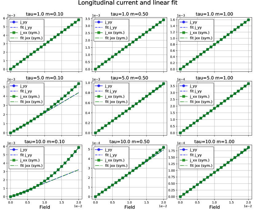
Figure 5: Steady-state longitudinal current $j_{y}(\bm{E}\parallel\hat{y})$ (blue circles) and symmetrized longitudinal current $j_{x}(\bm{E}\parallel\pm\hat{x})$ [see Eqs. (11a)] (green squares) with linear fits (dashed and dash-dotted) versus field amplitude for varying $\tau$ and $m$. Current in units $et_{h}/(\hbar a)$, field in units $t_{h}/(ea)$.

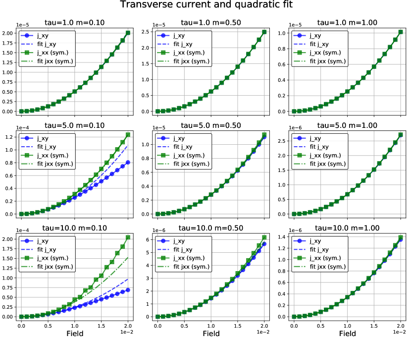
Figure 6: Steady-state transverse current $j_{x}(\bm{E}\parallel\hat{y})$ (blue circles) and symmetrized longitudinal current $j_{x}(\bm{E}\parallel\pm\hat{x})$ [see Eqs. (11b)] (green squares) with quadratic fits (dashed and dash-dotted) versus field amplitude for varying $\tau$ and $m$. Current in units $et_{h}/(\hbar a)$, field in units $t_{h}/(ea)$.

In Fig. 5 we plot the steady-state currents $j_{y}(\bm{E}\parallel\hat{y})$ and symmetrized $j_{x}(\bm{E}\parallel\pm\hat{x})$ cf. Eq. (11a) together with linear fits, similar to Fig. 2(c). Similarly, in Fig. 6 we plot the steady-state currents $j_{x}(\bm{E}\parallel\hat{y})$ and symmetrized $j_{x}(\bm{E}\parallel\pm\hat{x})$ cf. Eq. (11b) together with quadratic fits, similar to Fig. 2(d). Fixing a field-amplitude range, the power-series expansion Eq. (1) and the consequent Eq. (4) fail for small $m$ and large $\tau$. It is however possible, for any choice of finite $m$ and $\tau$, to take small enough $E$.