Efficient Multifidelity Likelihood-Free Bayesian Inference with Adaptive Computational Resource Allocation

Abstract

Likelihood-free Bayesian inference algorithms are popular methods for calibrating the parameters of complex, stochastic models, required when the likelihood of the observed data is intractable. These algorithms characteristically rely heavily on repeated model simulations. However, whenever the computational cost of simulation is even moderately expensive, the significant burden incurred by likelihood-free algorithms leaves them unviable in many practical applications. The multifidelity approach has been introduced (originally in the context of approximate Bayesian computation) to reduce the simulation burden of likelihood-free inference without loss of accuracy, by using the information provided by simulating computationally cheap, approximate models in place of the model of interest. The first contribution of this work is to demonstrate that multifidelity techniques can be applied in the general likelihood-free Bayesian inference setting. Analytical results on the optimal allocation of computational resources to simulations at different levels of fidelity are derived, and subsequently implemented practically. We provide an adaptive multifidelity likelihood-free inference algorithm that learns the relationships between models at different fidelities and adapts resource allocation accordingly, and demonstrate that this algorithm produces posterior estimates with near-optimal efficiency.

1 Introduction

Across domains in engineering and science, parametrised mathematical models are often too complex to analyse directly. Instead, many outer-loop applications [Peherstorfer et al., 2018], such as model calibration, optimization, and uncertainty quantification, rely on repeated simulation to understand the relationship between model parameters and behaviour. In time-sensitive and cost-aware applications, the typical computational burden of such simulation-based methods makes them impractical. Multifidelity methods, reviewed by Peherstorfer et al. [2016, 2018], are a family of approaches that exploit information gathered from simulations, not only of a single model of interest, but also of additional approximate or surrogate models. In this article, the term model refers to the underlying mathematical abstraction of a system in combination with the computer code used to implement simulations. Thus, ‘model approximation’ may refer to mathematical simplifications and/or approximations in numerical methods. The fundamental challenge when implementing multifidelity techniques is the allocation of computational resources between different models, for the purposes of balancing a characteristic trade-off between maintaining accuracy and saving computational burden.

In this work, we consider a specific outer-loop application that arises in Bayesian statistics, the goal of which is to calibrate a parametrised model against observed data. Bayesian inference uses the likelihood of the observed data to update a prior distribution on the model parameters into a posterior distribution, according to Bayes’s rule. In the situation where the likelihood of the data cannot be calculated, we rely on so-called likelihood-free methods that provide estimates of the likelihood by comparing model simulations to data. For example, approximate Bayesian computation (ABC) is a widely-known likelihood-free inference technique [Sisson et al., 2020, Sunnåker et al., 2013], where the likelihood is typically estimated as a binary value, recording whether or not the distance between a simulation and the observed data falls within a given threshold. Other likelihood-free methods are also available, such as pseudo-marginal methods and Bayesian synthetic likelihoods (BSL). In this work, we develop a generalised likelihood-free framework for which ABC, pseudo-marginal and BSL can be expressed as specific cases, as described in Section 2.1.

The significant cost of likelihood-free inference has motivated several successful proposals for improving the efficiency of likelihood-free samplers, such as (in the specific context of ABC) ABC-MCMC [Marjoram et al., 2003] and ABC-SMC [Sisson et al., 2007, Toni et al., 2009, Del Moral et al., 2011]. These approaches aim to efficiently explore parameter space by avoiding the proposal of low-likelihood parameters, reducing the required number of expensive simulations required and reducing the ABC rejection rate. However, an ‘orthogonal’ technique for improving the efficiency of likelihood-free inference is to instead ensure that each simulation-based likelihood estimate is, on average, less computationally expensive to generate.

In previous work, Prescott and Baker [2020, 2021] investigated multifidelity approaches to likelihood-free Bayesian inference [Cranmer et al., 2020], with a specific focus on ABC [Sisson et al., 2020, Sunnåker et al., 2013]. Suppose that there exists a low-fidelity approximation to the parametrised model of interest, and that the approximation is relatively cheap to simulate. Monte Carlo estimates of the posterior distribution, with respect to the likelihood of the original high-fidelity model, can be constructed using the simulation outputs of the low-fidelity approximation. Prescott and Baker [2020] showed that using the low-fidelity approximation introduces no further bias, so long as, for any parameter proposal, there is a positive probability of simulating the high-fidelity model to check and potentially correct a low-fidelity likelihood estimate. The key to the success of the multifidelity ABC (MF-ABC) approach is to choose this positive probability to be suitably small, thereby simulating the original model as little as possible, while ensuring it is large enough that the variance of the resulting Monte Carlo estimate is suitably small. The result of the multifidelity approach is to reduce the expected cost of estimating the likelihood for each parameter proposal in any Monte Carlo sampling algorithm. In subsequent work, Prescott and Baker [2021] showed that this approach integrates with sequential Monte Carlo (SMC) sampling for efficient parameter space exploration [Toni et al., 2009, Del Moral et al., 2011, Drovandi and Pettitt, 2011]. Thus, the synergistic effect of combining multifidelity and with SMC to improve the efficiency of ABC has been demonstrated.

Multifidelity ABC can be compared with previous techniques for exploiting model approximation in ABC, such as Preconditioning ABC [Warne et al., 2021a], Lazy ABC (LZ-ABC) [Prangle, 2016], and Delayed Acceptance ABC (DA-ABC) [Christen and Fox, 2005, Everitt and Rowińska, 2021]. Similarly to sampling techniques such as SMC, the preconditioning approach seeks to explore parameter space more efficiently, by proposing parameters for high-fidelity simulation with greater low-fidelity posterior mass. In contrast, each of MF-ABC, LZ-ABC, and DA-ABC seeks to make each parameter proposal quicker to evaluate, on average, by using the output of the low-fidelity simulation to directly decide whether to simulate the high-fidelity model. In both LZ-ABC and DA-ABC, a parameter proposal is either (a) rejected early, based on the simulated output of the low-fidelity model, or (b) sent to a high-fidelity simulation, to make a final decision on ABC acceptance or rejection. The distinctive aspect of MF-ABC is that step (a) is different; it is not necessary to reject early to avoid high-fidelity simulation. Instead the low-fidelity simulation can be used to make the accept/reject decision directly. In both DA-ABC and MF-ABC, the decision between (a) or (b) is based solely on whether the low-fidelity simulation would be accepted or rejected. In contrast, LZ-ABC allows for a much more generic decision of whether to simulate the high-fidelity model, requiring an extensive exploration of practical tuning methods.

In this paper, we will show that the multifidelity approach can be applied to any simulation-based likelihood-free inference methodology, including but not limited to ABC. We achieve this by developing a generalised framework for likelihood-free inference, and deriving a multifidelity method to operate in this framework. A successful multifidelity likelihood-free inference algorithm requires us to determine how many simulations of the high-fidelity model to perform, based on the parameter value and the simulated output of the low-fidelity model. We provide theoretical results and practical, automated tuning methods to allocate computational resources between two models, designed to optimise the performance of multifidelity likelihood-free importance sampling.

1.1 Outline

In Section 2 we review likelihood-free Bayesian inference through constructing a generalised likelihood-free framework. Section 3 shows how the theory underpinning MF-ABC, as introduced by Prescott and Baker [2020], can be applied in this general likelihood-free Bayesian context. We analyse the performance of the resulting multifidelity likelihood-free importance sampling algorithm. The main results of this paper are set out in Section 3.3, in which we determine the optimal allocation of computational resources between the two models to achieve the best possible performance of multifidelity inference. Section 4 explores how to practically allocate computation between model fidelities, by adaptively evolving the allocation in response to learned relationships between simulations at each fidelity across parameter space. We illustrate adaptive multifidelity inference by applying the algorithm to a simple biochemical network motif in Section 5. We show that, using a low-fidelity Michaelis–Menten approximation together with the exact model (both simulated using the exact algorithm of Gillespie [1977]) our adaptive implementation of multifidelity likelihood-free inference can achieve a quantifiable speed-up in constructing posterior estimates to a specified variance and with no additional bias. Code for this example, developed in Julia 1.6.2 [Bezanson et al., 2017], is available at github.com/tpprescott/mf-lf. Finally, in Section 6 we discuss how greater improvements may be achieved for more challenging inference tasks.

2 Likelihood-free inference

We consider a stochastic model of the data generating process, defined by a distribution with parametrised probability density function, $f(\cdot\mid\theta)$, where the parameter vector $\theta$ takes values in a parameter space $\Theta$. For any $\theta$, the model induces a probability density, denoted $f(y\mid\theta)$, on observable outputs, with $y$ taking values in an output space $\mathcal{Y}$. We note that the model is usually implemented in computer code to allow simulation, through which outputs $y\in\mathcal{Y}$ can be generated. We write $y\sim f(\cdot\mid\theta)$ to denote simulation of the model $f$ given parameter values $\theta$. Taking the experimentally observed data $y_{0}\in\mathcal{Y}$, we define the likelihood function to be a function of $\theta$ using the density, $\mathcal{L}(\theta)=f(y_{0}\mid\theta)$, of the observed data under this model.

Bayesian inference updates prior knowledge of the parameter values, $\theta\in\Theta$, which we encode in a prior distribution with density $\pi(\theta)$. The information provided by the experimental data, encoded in the likelihood function, $\mathcal{L}(\theta)$, is combined with the prior using Bayes’ rule to form a posterior distribution, with density

$$\pi(\theta\mid y_{0})=\frac{\mathcal{L}(\theta)\pi(\theta)}{Z},$$ (1)

where $Z=\int\mathcal{L}(\theta)\pi(\theta)\leavevmode\nobreak\ \mathrm{d}\theta$ normalises $\pi(\cdot\mid y_{0})$ to be a probability distribution on $\Theta$. For a given, arbitrary, integrable function $G:\Theta\rightarrow\mathbb{R}$, we take the goal of the inference task as the production of a Monte Carlo estimate of the posterior expectation,

$$\bar{G}=\mathbf{E}(G\mid y_{0})=\int_{\Theta}G(\theta)\pi(\theta\mid y_{0})\leavevmode\nobreak\ \mathrm{d}\theta,$$ (2)

conditioned on the observed data.

2.1 Approximating the likelihood with simulation

In most practical settings, models tend to be sufficiently complicated that calculating $\mathcal{L}(\theta)=f(y_{0}\mid\theta)$ for $\theta\in\Theta$ is intractable. In this case, we exploit the ability to produce independent simulations from the model,

$$\mathbf{y} =(y_{1},\dots,y_{K}),$$ (3a)

$$y_{k} \sim f(\cdot\mid\theta).$$ (3b)

In the following, we will slightly abuse notation by using the shorthand $$\mathbf{y}\sim f(\cdot\mid\theta) K f(\cdot\mid\theta)$$ to represent independent, identically distributed draws from the parametrised distribution .

Given the observed data, $y_{0}$, we can define a real-valued function, referred to as a likelihood-free weighting,

$$\omega:(\theta,\mathbf{y})\mapsto\mathbb{R},$$ (3c)

which varies over the joint space of parameter values and simulation outputs. Here, $\omega$ is a function of a parameter value, $\theta$, and a vector, $\mathbf{y}$, of stochastic simulations. For a fixed $\theta$, we can take conditional expectations of $\omega(\theta,\mathbf{y})$ over the probability density of simulations, $f(\mathbf{y}\mid\theta)$, to define an approximate likelihood function,

$$L_{\omega}(\theta)=\mathbf{E}(\omega\mid\theta)=\int\omega(\theta,\mathbf{y})f(\mathbf{y}\mid\theta)\leavevmode\nobreak\ \mathrm{d}\mathbf{y},$$ (4a)

where $$L_{\omega}(\theta) \mathcal{L}(\theta) \theta \omega(\theta,\mathbf{y}) K \mathbf{y}\sim f(\cdot\mid\theta) L_{\omega}(\theta)$$ is assumed to be approximately equal to the modelled likelihood function, , up to a constant of proportionality. Note that, given , the random value of the likelihood-free weighting, , determined by stochastic simulations, , is a Monte Carlo estimate of the approximate likelihood function, .

The approximate likelihood function is used to define the likelihood-free approximation to the posterior,

$$\pi_{\omega}(\theta\mid y_{0})=\frac{L_{\omega}(\theta)\pi(\theta)}{Z_{\omega}},$$ (4b)

where the normalisation constant $Z_{\omega}=\int L_{\omega}(\theta)\pi(\theta)\leavevmode\nobreak\ \mathrm{d}\theta$ ensures that $\pi_{\omega}$ is a probability distribution. The likelihood-free approximation to the posterior, $\pi_{\omega}(\theta\mid y_{0})$, subsequently induces a biased estimate of $\bar{G}$, given by

$$\bar{G}_{\omega}=\mathbf{E}_{\pi_{\omega}}(G\mid y_{0})=\int G(\theta)\pi_{\omega}(\theta\mid y_{0})\leavevmode\nobreak\ \mathrm{d}\theta.$$ (4c)

In this situation, the success of likelihood-free inference depends on ensuring that the likelihood-free weighting, $\omega(\theta,\mathbf{y})$ is chosen such that the squared difference $(\bar{G}-\bar{G}_{\omega})^{2}$ between the posterior expectation, $\bar{G}$, and its likelihood-free approximation, $\bar{G}_{\omega}$, is as small as possible.

2.1.1 Example: ABC

Approximate Bayesian computation (ABC) is a widely-used example of likelihood-free inference, where

$$\omega_{\mathrm{ABC}}(\theta,\mathbf{y})=\frac{1}{K}\sum_{k=1}^{K}\mathbf{I}(d(y_{k},y_{0})\leq\epsilon),$$

is the random fraction of $K$ simulations, $y_{k}$, which are within a distance of $\epsilon$ of the observed data, as measured by the metric $d$. Sisson et al. [2007, 2020] note that it is standard practice to choose $K=1$. Taking the conditional expectation of $\omega_{\mathrm{ABC}}$, given $\theta$, this likelihood-free weighting induces the ABC approximation to the likelihood,

$$L_{\mathrm{ABC}}(\theta)=\mathbf{E}(\omega_{\mathrm{ABC}}\mid\theta)=\mathbf{P}(d(y,y_{0})\leq\epsilon\mid\theta),$$

for any $K$. Under appropriate choices of $d$ and $\epsilon$, the approximate likelihood function, $L_{\mathrm{ABC}}(\theta)$, may be considered approximately proportional to the likelihood, $\mathcal{L}(\theta)$.

2.1.2 Example: Bayesian synthetic likelihood

The simplest implementation of the Bayesian synthetic likelihood approach replaces the true likelihood with a Monte Carlo likelihood-free weighting based on a Gaussian density,

$$\omega_{\mathrm{SL}}(\theta,\mathbf{y})=\mathcal{N}(y_{0};\mu(\mathbf{y}),\Sigma^{2}(\mathbf{y})),$$

with random mean, $\mu=\sum_{k}y_{k}/K$, and covariance, $\Sigma^{2}=\sum_{k}(y_{k}-\mu)(y_{k}-\mu)^{T}/K$, given by the empirical mean and covariance of $K$ simulations. Taking conditional expectations of $\omega_{\mathrm{SL}}$, given $\theta$, induces the Bayesian synthetic likelihood, $L_{\mathrm{SL}}(\theta)=\mathbf{E}(\omega_{\mathrm{SL}}(\theta,\mathbf{y})\mid\theta)$, as an approximation of the likelihood, $\mathcal{L}(\theta)$.

2.1.3 Example: Pseudo-marginal method

For the pseudo-marginal approach, introduced by Andrieu and Roberts [2009], we suppose that there exists a simulation-based estimator, $\omega(\theta,\mathbf{y})$, such that the conditional expectation $L_{\omega}(\theta)=\mathbf{E}(\omega\mid\theta)$ is an unbiased estimate of $\mathcal{L}(\theta)=f(y_{0}\mid\theta)$. For example, following Warne et al. [2020], suppose that an intractable density $f(y\mid\theta)$ arising from a stochastic model can be decomposed into an underlying latent model, $x\sim g(\cdot\mid\theta)$, and an observation model, $y\sim h(\cdot\mid\theta,x)$, such that $f(y\mid\theta)=\int h(y\mid\theta,x)g(x\mid\theta)\mathrm{d}x$. Assume that the probability densities $h(y\mid\theta,x)$ of the observation model can be calculated. Then, for simulations $x_{k}\sim g(\cdot\mid\theta)$ of the latent model, where $k=1,\dots,K$, we can write

$$\omega(\theta,\mathbf{x})=\frac{1}{K}\sum_{k}h(y_{0}\mid\theta,x_{k}),$$

as a likelihood-free weighting. Taking expectations over $\mathbf{x}\sim g(\cdot\mid\theta)$, we have $L_{\omega}(\theta)=\mathbf{E}(\omega\mid\theta)=f(y_{0}\mid\theta)=\mathcal{L}(\theta)$. Thus, $L_{\omega}(\theta)$ is an exact approximation [Drovandi et al., 2019].

2.2 Likelihood-free importance sampling

A simple approach to estimating the likelihood-free approximate posterior mean, $\bar{G}_{\omega}$, is to use importance sampling. We assume that parameter proposals $\theta_{i}\sim q(\cdot)$, for $i=1,\dots,N$, can be sampled from a given importance distribution, the support of which must include the prior support. In practice, we need only know importance density values, $q(\theta)$, up to a multiplicative constant, but for simplicity we assume that $q(\theta)$ is known. We also assume that we have access to the prior probability density, $\pi(\theta)$.

The likelihood-free importance sampling algorithm is described in Algorithm 1. This algorithm requires the specification of an importance distribution, $q$, and a likelihood-free weighting, $\omega(\theta,\mathbf{y})$, with conditional expectation, $L_{\omega}(\theta)=\mathbf{E}(\omega\mid\theta)$. The output of Algorithm 1, $\hat{G}$, is an estimate of the likelihood-free approximate posterior expectation, $\bar{G}_{\omega}=\mathbf{E}_{\pi_{\omega}}(G\mid y_{0})$. In 1, we prove the standard result that $\hat{G}$ is a consistent estimate of $\bar{G}_{\omega}$, and quantify the dominant behaviour of the mean squared error in the limit of large sample sizes, $N\rightarrow\infty$. For notational simplicity, we define the function $\Delta(\theta)=G(\theta)-\bar{G}_{\omega}$ to recentre $G$ at the approximate posterior mean, and denote the Monte Carlo error between $\hat{G}$ and $\bar{G}_{\omega}$ as the estimated mean value of $\Delta$, denoted by $\hat{\Delta}=\hat{G}-\bar{G}_{\omega}$.

Algorithm 1 Likelihood-free importance sampling.

Prior, $\pi$; importance distribution, $q$; likelihood-free weighting, $\omega$; model $f(\cdot\mid\theta)$; stop condition, stop; target function, $G$.

Set counter $i=0$.

repeat

     Increment counter $i\leftarrow i+1$;

     Sample $\theta_{i}\sim q(\cdot)$;

     Simulate $\mathbf{y}_{i}\sim f(\cdot\mid\theta_{i})$;

     Calculate weight,

$$w_{i}=w(\theta_{i},\mathbf{y}_{i})=\frac{\pi(\theta_{i})}{q(\theta_{i})}\omega(\theta_{i},\mathbf{y}_{i});$$ (5)

until stop = true

return Weighted sum,

$$\hat{G}=\sum_{i=1}^{N}w_{i}G(\theta_{i})\bigg{/}\sum_{j=1}^{N}w_{j}.$$

Theorem 1.

For the weighted sample values $(\theta_{i},w_{i})$ produced in each iteration of Algorithm 1, let $w$ denote the random value of the weight $w_{i}$, and let $\Delta$ denote the random value of $\Delta(\theta_{i})$. The mean squared error (MSE) of the output, $\hat{G}$, of Algorithm 1, as an estimator for the approximate posterior expectation, $\bar{G}_{\omega}$, is given to leading order by

$$\mathbf{E}\left(\hat{\Delta}^{2}\right)=\left[\frac{\mathbf{E}\left(w^{2}\Delta^{2}\right)}{\mathbf{E}(w)^{2}}\right]\frac{1}{N}+O\left(\frac{1}{N^{2}}\right).$$ (6)

Thus, $\hat{G}$ is a consistent estimator of $\bar{G}_{\omega}$.

Proof.

The Monte Carlo estimate produced by Algorithm 1, $\hat{G}=R/S$, is the ratio of two random variables: the weighted sum, $R=\sum_{i=1}^{N}w(\theta_{i},\mathbf{y}_{i})G(\theta_{i})$, and the normalising sum, $S=\sum_{i=1}^{N}w(\theta_{i},\mathbf{y}_{i})$. We write the function $\Phi(r,s)=(r/s-\bar{G}_{\omega})^{2}$, and note that the MSE is the expected value of the function $\hat{\Delta}^{2}=\Phi(R,S)$. Using the delta method, we take expectations of the second-order Taylor expansion of $\Phi(R,S)$ about $(\mu_{R},\mu_{S})=(\mathbf{E}(R),\mathbf{E}(S))$, to give

$$\mathbf{E}\left(\hat{\Delta}^{2}\right)=\mathbf{E}\left(\Phi(R,S)\right) =\Phi(\mu_{R},\mu_{S})$$

$$\quad+\frac{1}{\mu_{S}^{2}}\left[\mathrm{Var}(R)+\left(2\bar{G}_{\omega}-\frac{4\mu_{R}}{\mu_{S}}\right)\mathrm{Cov}(R,S)+\left(\frac{3\mu_{R}-2\bar{G}_{\omega}\mu_{S}}{\mu_{S}^{2}}\right)\mu_{R}\mathrm{Var}(S)\right]$$

$$\quad+O\left(\frac{\mathbf{E}\left(\left(\left(R-\mu_{R}\right)+\left(S-\mu_{S}\right)\right)^{3}\right)}{\mu_{s}^{3}}\right).$$

Taking expectations with respect to $N$ independent draws of $(\theta,\mathbf{y})$ with density $f(\mathbf{y}\mid\theta)q(\theta)$, it is straightforward to write

$$\mu_{R}=\mathbf{E}(R) =N\mathbf{E}(wG)=NZ_{\omega}\bar{G}_{\omega},$$

$$\mu_{S}=\mathbf{E}(S) =N\mathbf{E}(w)=NZ_{\omega},$$

where we recall that $\mathbf{E}(w)=Z_{\omega}=\int L_{\omega}(\theta)\pi(\theta)\leavevmode\nobreak\ \mathrm{d}\theta$ is the normalising constant in Equation 4b. We substitute these expectations into the Taylor expansion of $\mathbf{E}(\hat{\Delta}^{2})$, noting that the leading-order term, $\Phi(\mu_{R},\mu_{S})$, is zero. Thus, we can write the dominant behaviour of the MSE as

$$\mathbf{E}\left(\hat{\Delta}^{2}\right) =\frac{1}{N^{2}Z_{\omega}^{2}}\left[\mathrm{Var}(R)-2\bar{G}_{\omega}\mathrm{Cov}(R,S)+\bar{G}_{\omega}^{2}\mathrm{Var}(S)\right]+O\left(\frac{\mathbf{E}\left(\left(\left(R-\mu_{R}\right)+\left(S-\mu_{S}\right)\right)^{3}\right)}{N^{3}}\right)$$

$$=\frac{1}{N^{2}Z_{\omega}^{2}}\mathrm{Var}(R-\bar{G}_{\omega}S)+O\left(\frac{\mathbf{E}\left(\left(\left(R-\mu_{R}\right)+\left(S-\mu_{S}\right)\right)^{3}\right)}{N^{3}}\right),$$

as $N\rightarrow\infty$. Substituting into this expression the definitions of $R$ and $S$ as summations of $N$ independent identically distributed random variables, we have

$$\mathbf{E}(\hat{\Delta}^{2})=\frac{1}{N^{2}Z_{\omega}^{2}}N\mathrm{Var}(w\Delta)+O\left(\frac{N}{N^{3}}\right),$$

and Equation 6 follows, on noting that $\mathbf{E}(w\Delta)=0$ and that $\mathbf{E}(w)=Z_{\omega}$. ∎

1 determines the leading-order behaviour of the MSE of the output of Algorithm 1 in terms of sample size. We can also quantify the performance of this algorithm in terms of how the MSE decreases with increasing the overall computational budget.

Corollary 2.

Let the computational cost of each iteration of Algorithm 1 be denoted by the random variable $C$. The leading order behaviour of the MSE of $\hat{G}$ as an estimate of $\bar{G}_{\omega}$ is

$$\mathbf{E}\left(\hat{\Delta}^{2}\right)=\left[\frac{\mathbf{E}(C)\mathbf{E}\left(w^{2}\Delta^{2}\right)}{\mathbf{E}(w)^{2}}\right]\frac{1}{C_{\mathrm{tot}}}+O\left(\frac{1}{C_{\mathrm{tot}}^{2}}\right),$$ (7)

as the total simulation budget $C_{\mathrm{tot}}\rightarrow\infty$.

Proof.

As the given computational budget increases, $C_{\mathrm{tot}}\rightarrow\infty$, the Monte Carlo sample size that can be produced in that budget increases on the order of $N\sim C_{\mathrm{tot}}/\mathbf{E}(C)$. On substituting this expression into Equation 6, the result follows. ∎

We can use the leading-order coefficient of $1/C_{\mathrm{tot}}$ in Equation 7 to quantify the performance of likelihood-free importance sampling. Importantly, this expression explicitly depends on the expected computational cost, $C$, of each iteration of Algorithm 1. In the importance sampling context, the optimal importance distribution $q$ should seek to minimise this coefficient, by trading off a preference for parameter values with lower computational burden against ensuring small variability in the weighted errors, $w\Delta$. However, for simplicity, we will assume in this paper that $q$ is fixed. Instead, we seek ways to use model approximations to directly reduce the leading-order coefficient in Equation 7, based on the identified trade-off between decreasing computational burden, $C$, and controlling the variance of the weighted error, $w\Delta$.

3 Multifidelity inference

In 2, the performance of Algorithm 1 is quantified explicitly in terms of how the Monte Carlo error between the estimate, $\hat{G}$, and the approximated posterior mean, $\bar{G}_{\omega}$, decays with increasing computational budget, $C_{\mathrm{tot}}$. It initially appears reasonable to conclude that the linear dependence of the performance on the expected iteration time, $\mathbf{E}(C)$, implies that if we can speed up the simulation step of Algorithm 1, then we can significantly reduce the MSE for a given computational budget.

Suppose that there exists an alternative model that we can use in Algorithm 1 in place of the original model, $f(\cdot\mid\theta)$, such that the expected computation time for each iteration, $\mathbf{E}(C)$, is significantly reduced. There are two important issues that prevent this being a viable option for improving the efficiency of likelihood-free inference. The first problem is that we need to be able to quantify the effect of the alternative model on the ratio $\mathbf{E}(w^{2}\Delta^{2})/\mathbf{E}(w)^{2}$ to ensure that the overall performance of the algorithm is improved. It is not sufficient to show that the computational burden of each iteration is reduced, if too many more iterations are subsequently required to achieve a specified MSE.

The second problem arises from the observation that the limiting value of $\hat{G}$, as output from Algorithm 1, is $\bar{G}_{\omega}$, with residual bias,

$$\lim_{C_{\mathrm{tot}}\rightarrow\infty}\mathbf{E}\left(\left(\hat{G}-\bar{G}\right)^{2}\right)=(\bar{G}_{\omega}-\bar{G})^{2}\neq 0,$$

recalling that $\bar{G}_{\omega}$ is the approximate posterior expectation induced by $L_{\omega}(\theta)=\mathbf{E}(\omega\mid\theta)$, and where the approximand, $\bar{G}$, is the posterior expectation induced by the likelihood, $\mathcal{L}(\theta)=f(y_{0}\mid\theta)$. We will identify this limiting residual squared bias, $(\bar{G}_{\omega}-\bar{G})^{2}$, as the fidelity of the model/likelihood-free weighting pair. We emphasise here that the fidelity depends both on the model and the likelihood-free weighting used in Algorithm 1, and is contextual to the target function, $G$. For a given posterior mean, $\bar{G}$, a model and likelihood-free weighting pair for which the value of $(\bar{G}_{\omega}-\bar{G})^{2}$ is small is termed high-fidelity, while larger values of $(\bar{G}_{\omega}-\bar{G})^{2}$ are termed low-fidelity. Thus, if we use an alternative model in place of $f$ in Algorithm 1, the model (and likelihood-free weighting) may be too low-fidelity, in the sense of having too large a residual squared bias versus the posterior expectation of interest, $\bar{G}$.

The multifidelity framework overcomes both these problems, by removing the need for a binary choice between the expensive model of interest and its cheaper alternative. Instead, we carry out likelihood-free inference using information from both models. We introduce the multifidelity likelihood-free importance sampling algorithm in Section 3.1. In Section 3.2, we show that multifidelity likelihood-free importance sampling loses no fidelity versus high-fidelity importance sampling. Section 3.3 contains the main analytical results of this paper, in which we explore the conditions under which multifidelity inference can improve the performance of likelihood-free importance sampling with finite computational budgets, as quantified by the leading-order characterisation of the MSE given in Equation 7.

3.1 Multifidelity likelihood-free importance sampling

We denote the high-fidelity model and likelihood-free weighting as $f_{\mathrm{hi}}$ and $\omega_{\mathrm{hi}}$, respectively. The likelihood under the high-fidelity model is denoted $\mathcal{L}_{\mathrm{hi}}(\theta)=f_{\mathrm{hi}}(y_{0}\mid\theta)$, and is assumed to be intractable. Following the notation introduced in Equation 4, the high-fidelity pair $f_{\mathrm{hi}}$ and $\omega_{\mathrm{hi}}$ induce the approximate likelihood, $L_{\mathrm{hi}}(\theta)=\mathbf{E}(\omega_{\mathrm{hi}}\mid\theta)$ and the corresponding likelihood-free approximation to the posterior expectation, $\bar{G}_{\mathrm{hi}}$. We further assume that simulating each $\mathbf{y}_{\mathrm{hi}}\sim f_{\mathrm{hi}}(\cdot\mid\theta)$ is computationally expensive. This computational expense motivates the use of an approximate, low-fidelity model and likelihood-free weighting, denoted $f_{\mathrm{lo}}$ and $\omega_{\mathrm{lo}}$, respectively, inducing the approximate likelihood, $L_{\mathrm{lo}}(\theta)=\mathbf{E}(\omega_{\mathrm{lo}}\mid\theta)$, and corresponding likelihood-free approximation to the posterior expectation, $\bar{G}_{\mathrm{lo}}$. We note that the low-fidelity model, $f_{\mathrm{lo}}$, induces its own likelihood, $L_{\mathrm{lo}}=f_{\mathrm{lo}}(y_{0}\mid\theta)$, but assume that this remains intractable, requiring instead the simulation-based Bayesian approach. However, we assume that simulations of the low-fidelity model, $\mathbf{y}_{\mathrm{lo}}\sim f_{\mathrm{lo}}(\cdot\mid\theta)$, are significantly cheaper to produce compared to simulations of the high-fidelity model.

Given the models $f_{\mathrm{lo}}$ and $f_{\mathrm{hi}}$, we will term the joint distribution $f_{\mathrm{mf}}(\mathbf{y}_{\mathrm{lo}},\mathbf{y}_{\mathrm{hi}}\mid\theta)$ a multifidelity model when $f_{\mathrm{mf}}$ has marginals equal to the low- and high-fidelity densities, $f_{\mathrm{lo}}(\mathbf{y}_{\mathrm{lo}}\mid\theta)$ and $f_{\mathrm{hi}}(\mathbf{y}_{\mathrm{hi}}\mid\theta)$. The models may be conditionally independent, such that $f_{\mathrm{mf}}(\mathbf{y}_{\mathrm{lo}},\mathbf{y}_{\mathrm{hi}}\mid\theta)=f_{\mathrm{lo}}(\mathbf{y}_{\mathrm{lo}}\mid\theta)f_{\mathrm{hi}}(\mathbf{y}_{\mathrm{hi}}\mid\theta)$, in which case simulations at each model fidelity can be carried out independently given $\theta$. Furthermore, if the simulations are conditionally independent, this means that the resulting likelihood-free weights, $\omega_{\mathrm{lo}}(\theta,\mathbf{y}_{\mathrm{lo}})$ and $\omega_{\mathrm{hi}}(\theta,\mathbf{y}_{\mathrm{hi}})$, are also conditionally independent.

However, in the more general definition of the multifidelity model as a joint distribution, we allow for coupling between the two fidelities. Conditioned on the low-fidelity simulations, $\mathbf{y}_{\mathrm{lo}}$, and on parameter values, $\theta$, we can produce a coupled simulation, $\mathbf{y}_{\mathrm{hi}}$, from the density $f_{\mathrm{hi}}(\mathbf{y}_{\mathrm{hi}}\mid\theta,\mathbf{y}_{\mathrm{lo}})$ implied by

$$f_{\mathrm{mf}}(\mathbf{y}_{\mathrm{lo}},\mathbf{y}_{\mathrm{hi}}\mid\theta)=f_{\mathrm{hi}}(\mathbf{y}_{\mathrm{hi}}\mid\theta,\mathbf{y}_{\mathrm{lo}})f_{\mathrm{lo}}(\mathbf{y}_{\mathrm{lo}}\mid\theta).$$

Coupling imposes correlations between the resulting likelihood-free weights, $\omega_{\mathrm{lo}}(\theta,\mathbf{y}_{\mathrm{lo}})$ and $\omega_{\mathrm{hi}}(\theta,\mathbf{y}_{\mathrm{hi}})$, which thus allows evaluated values of $\omega_{\mathrm{lo}}$ to provide more information about unknown values of $\omega_{\mathrm{hi}}$, thereby acting as a variance reduction technique [Owen, 2013]. Given the (coupled) multifidelity model, we can calculate a multifidelity likelihood-free weighting as follows.

Definition 3.

Let $M$ be any non-negative integer-valued random variable, with conditional probability mass function $p(\cdot\mid\theta,\mathbf{y}_{\mathrm{lo}})$, and with a positive conditional mean,

$$\mu(\theta,\mathbf{y}_{\mathrm{lo}})=\mathbf{E}(M\mid\theta,\mathbf{y}_{\mathrm{lo}})>0.$$

Given a parameter value, $\theta$, we define

$$\mathbf{z} =(\mathbf{y}_{\mathrm{lo}},\mathbf{y}_{\mathrm{hi},1},\mathbf{y}_{\mathrm{hi},2},\dots,\mathbf{y}_{\mathrm{hi},m}),$$ (8a)

$$\mathbf{y}_{\mathrm{lo}} \sim f_{\mathrm{lo}}(\cdot\mid\theta),$$ (8b)

$$m \sim p(\cdot\mid\theta,\mathbf{y}_{\mathrm{lo}}),$$ (8c)

$$\mathbf{y}_{\mathrm{hi},i} \sim f_{\mathrm{hi}}(\cdot\mid\theta,\mathbf{y}_{\mathrm{lo}}),$$ (8d)

noting that each $$\mathbf{y}_{\mathrm{hi},i} \mathbf{y}_{\mathrm{lo}}\sim f_{\mathrm{lo}}(\cdot\mid\theta) \mathbf{z} \phi(\mathbf{z}\mid\theta)$$ may be coupled to the low-fidelity simulation . We combine Equations 8a, 8b, 8c and 8d to write the density of as . We further define the multifidelity likelihood-free weighting function,

$$\omega_{\mathrm{mf}}(\theta,\mathbf{z}) =\omega_{\mathrm{lo}}(\theta,\mathbf{y}_{\mathrm{lo}})$$

$$\quad+\frac{1}{\mu(\theta,\mathbf{y}_{\mathrm{lo}})}\sum_{i=1}^{m}\left[\omega_{\mathrm{hi}}(\theta,\mathbf{y}_{\mathrm{hi},i})-\omega_{\mathrm{lo}}(\theta,\mathbf{y}_{\mathrm{lo}})\right],$$ (8e)

as the low-fidelity likelihood-free weighting, corrected by a randomly drawn number, $$M=m \mathbf{z}$$, of conditionally independent high-fidelity likelihood-free weightings. Taking expectations over , we write

$$L_{\mathrm{mf}}(\theta)=\mathbf{E}(\omega_{\mathrm{mf}}\mid\theta)=\int\omega_{\mathrm{mf}}(\theta,\mathbf{z})\phi(\mathbf{z}\mid\theta)\leavevmode\nobreak\ \mathrm{d}\mathbf{z},$$ (8f)

as the multifidelity approximation to the likelihood.

Given $M=m$, only $m$ replicates of $\mathbf{y}_{\mathrm{hi},i}\sim f_{\mathrm{hi}}(\cdot\mid\theta,\mathbf{y}_{\mathrm{lo}})$ need to be simulated for $\omega_{\mathrm{mf}}(\theta,\mathbf{z})$ to be evaluated. Thus, whenever $m=0$, this means that no high-fidelity simulations need to be completed for $\omega_{\mathrm{mf}}(\theta,\mathbf{z})$ to be calculated, removing the high-fidelity simulation cost from that iteration. Algorithm 2 presents the adaptation of the basic importance sampling method of Algorithm 1 to incorporate the multifidelity weighting function. The simulation step, $\mathbf{y}\sim f(\cdot\mid\theta)$, in Algorithm 1 is replaced by the MF-Simulate function in Algorithm 2.

Algorithm 2 Multifidelity likelihood-free importance sampling.

Prior, $\pi$; importance distribution, $q$; likelihood-free weightings, $\omega_{\mathrm{hi}}$ and $\omega_{\mathrm{lo}}$; models $f_{\mathrm{hi}}(\cdot\mid\theta)$ and $f_{\mathrm{lo}}(\cdot\mid\theta)$; conditional probability mass function $p(\cdot\mid\theta,\mathbf{y}_{\mathrm{lo}})$ on non-negative integers with mean function $\mu(\theta,\mathbf{y}_{\mathrm{lo}})$; stop condition, stop; target estimated function, $G$.

Set counter $i=0$.

repeat

     Increment counter $i\leftarrow i+1$;

     Sample $\theta_{i}\sim q(\cdot)$;

     Generate $\mathbf{z}_{i}\sim\phi(\cdot\mid\theta_{i})$ from MF-Simulate($\theta_{i}$);

     For $\omega_{\mathrm{mf}}$ in Equation 8e, calculate the weight

$$w_{i}=w_{\mathrm{mf}}(\theta,\mathbf{z}_{i})=\frac{\pi(\theta_{i})}{q(\theta_{i})}\omega_{\mathrm{mf}}(\theta_{i},\mathbf{z}_{i}).$$ (9)

until stop = true

return Weighted sum,

$$\hat{G}_{\mathrm{mf}}=\sum_{i=1}^{N}w_{i}G(\theta_{i})\bigg{/}\sum_{j=1}^{N}w_{j}.$$

function MF-Simulate($\theta$)

     Simulate $\mathbf{y}_{\mathrm{lo}}\sim f_{\mathrm{lo}}(\cdot\mid\theta)$;

     Generate $m\sim p(\cdot\mid\theta,\mathbf{y}_{\mathrm{lo}})$ with mean $\mu(\theta,\mathbf{y}_{\mathrm{lo}})$;

     if $m=0$ then

         return $\mathbf{z}=(\mathbf{y}_{\mathrm{lo}})$;

     else

         for $i=1,\dots,m$ do

              Simulate $\mathbf{y}_{\mathrm{hi},i}\sim f_{\mathrm{hi}}(\cdot\mid\theta,\mathbf{y}_{\mathrm{lo}})$;          

         return $\mathbf{z}=(\mathbf{y}_{\mathrm{lo}},\mathbf{y}_{\mathrm{hi},1},\dots,\mathbf{y}_{\mathrm{hi},m})$      

3.2 Accuracy of multifidelity inference

We observe that using $f_{\mathrm{hi}}$ and $\omega_{\mathrm{hi}}$ in Algorithm 1 produces an estimate of the high-fidelity approximate posterior expectation, $\bar{G}_{\mathrm{hi}}$. In 4, we show that the multifidelity approximate likelihood, $L_{\mathrm{mf}}(\theta)=\mathbf{E}(\omega_{\mathrm{mf}}(\theta,\mathbf{z})\mid\theta)$, is equal to the high-fidelity approximate likelihood, $L_{\mathrm{hi}}(\theta)=\mathbf{E}(\omega_{\mathrm{hi}}(\theta,\mathbf{y}_{\mathrm{hi}})\mid\theta)$. As a result, Algorithm 2 also produces a consistent estimate of the high-fidelity approximate posterior expectation, $\bar{G}_{\mathrm{hi}}$.

Proposition 4.

The multifidelity approximation to the likelihood, $L_{\mathrm{mf}}(\theta)=\mathbf{E}(\omega_{\mathrm{mf}}\mid\theta)$, is equal to the high-fidelity approximation to the likelihood, $L_{\mathrm{hi}}(\theta)=\mathbf{E}(\omega_{\mathrm{hi}}\mid\theta)$. Therefore, the estimate $\hat{G}_{\mathrm{mf}}$ produced by Algorithm 2 is a consistent estimate of the high-fidelity approximate posterior expectation, $\bar{G}_{\mathrm{hi}}$.

Proof.

We take the expectation of $\omega_{\mathrm{mf}}$ conditional on $(\theta,\mathbf{y}_{\mathrm{lo}},m)$, to find

$$\mathbf{E}(\omega_{\mathrm{mf}}\mid\theta,\mathbf{y}_{\mathrm{lo}},M=m)=\left(1-\frac{m}{\mu}\right)\omega_{\mathrm{lo}}(\theta,\mathbf{y}_{\mathrm{lo}})+\frac{m}{\mu}\mathbf{E}(\omega_{\mathrm{hi}}\mid\theta,\mathbf{y}_{\mathrm{lo}}).$$

Further taking expectations over the random integer $M$, which has conditional expected value $\mu(\theta,\mathbf{y}_{\mathrm{lo}})$, gives

$$\mathbf{E}(\omega_{\mathrm{mf}}\mid\theta,\mathbf{y}_{\mathrm{lo}})=\mathbf{E}(\omega_{\mathrm{hi}}\mid\theta,\mathbf{y}_{\mathrm{lo}}).$$

Further taking expectations with respect to $\mathbf{y}_{\mathrm{lo}}$, it follows that $L_{\omega_{\mathrm{mf}}}(\theta)=L_{\omega_{\mathrm{hi}}}(\theta)$. Therefore, the likelihood-free approximate posteriors, $\pi_{\omega_{\mathrm{mf}}}=\pi_{\omega_{\mathrm{hi}}}$, are equal and thus $\hat{G}_{\mathrm{mf}}$ is a consistent estimate of $\bar{G}_{\omega_{\mathrm{mf}}}=\bar{G}_{\omega_{\mathrm{hi}}}$, as required. ∎

In the limit of infinite computational budgets, the estimate produced by multifidelity importance sampling, in Algorithm 2, is as accurate as the estimate produced by high-fidelity importance sampling, in Algorithm 1 using $f_{\mathrm{hi}}$ and $\omega_{\mathrm{hi}}$. However, we still need to show that the performance of Algorithm 2 exceeds that of Algorithm 1 in the practical context of limited computational budgets. In Section 3.3, we introduce a method to quantify the performance of Algorithms 1 and 2 and show that the performance of multifidelity inference is strongly determined by the distribution of $M$, the random number of high-fidelity simulations required at each iteration.

3.3 Comparing performance

2 determines the leading-order behaviour of the MSE of the output of Algorithm 1 as the computational budget increases. A similar result applies to the output of Algorithm 2. We compare two settings: first, using Algorithm 1 with the high-fidelity model, $f_{\mathrm{hi}}$, and likelihood-free weighting, $\omega_{\mathrm{hi}}$. Each iteration has computational cost denoted $C_{\mathrm{hi}}$, and produces a weighted Monte Carlo sample with weights $w_{i}$ as independent draws of the random variable $w_{\mathrm{hi}}$. The output of Algorithm 1 is denoted $\hat{G}_{\mathrm{hi}}$, with Monte Carlo error $\hat{\Delta}_{\mathrm{hi}}=\hat{G}_{\mathrm{hi}}-\bar{G}_{\mathrm{hi}}$. The MSE for Algorithm 1 has leading-order behaviour

$$\mathbf{E}\left(\hat{\Delta}_{\mathrm{hi}}^{2}\right)=\left[\frac{\mathbf{E}(C_{\mathrm{hi}})\mathbf{E}\left(w_{\mathrm{hi}}^{2}\Delta^{2}\right)}{\mathbf{E}(w_{\mathrm{hi}})^{2}}\right]\frac{1}{C_{\mathrm{tot}}}+O\left(\frac{1}{C_{\mathrm{tot}}^{2}}\right),$$ (10)

as the total simulation budget $C_{\mathrm{tot}}\rightarrow\infty$, where $\Delta(\theta)=G(\theta)-\bar{G}_{\mathrm{hi}}$.

Second, we use Algorithm 2 with the multifidelity model $f_{\mathrm{mf}}$ and likelihood-free weighting, $\omega_{\mathrm{mf}}$. Each iteration has computational cost denoted $C_{\mathrm{mf}}$, and produces a weighted Monte Carlo sample with weights $w_{i}$ as independent draws of the random variable $w_{\mathrm{mf}}$. The output of Algorithm 2 is $\hat{G}_{\mathrm{mf}}$, with Monte Carlo error $\hat{\Delta}_{\mathrm{mf}}=\hat{G}_{\mathrm{mf}}-\bar{G}_{\mathrm{hi}}$. The MSE for Algorithm 2 has leading-order behaviour

$$\mathbf{E}\left(\hat{\Delta}_{\mathrm{mf}}^{2}\right)=\left[\frac{\mathbf{E}(C_{\mathrm{mf}})\mathbf{E}\left(w_{\mathrm{mf}}^{2}\Delta^{2}\right)}{\mathbf{E}(w_{\mathrm{mf}})^{2}}\right]\frac{1}{C_{\mathrm{tot}}}+O\left(\frac{1}{C_{\mathrm{tot}}^{2}}\right),$$ (11)

as the total simulation budget $C_{\mathrm{tot}}\rightarrow\infty$, where again $\Delta(\theta)=G(\theta)-\bar{G}_{\mathrm{hi}}$.

The main result of the paper is given in 5. For concreteness, we assume that the random variable, $M$, determining the required number of high-fidelity simulations in each iteration of Algorithm 2, is Poisson distributed, conditional on the parameter value and low-fidelity simulation output. We show that, for a given multifidelity model and likelihood-free weightings, the mean function, $\mu$, for $M$ determines the performance of Algorithm 2 relative to Algorithm 1.

Theorem 5.

Assume that the random number of high-fidelity simulations, $M$, required in each iteration of Algorithm 2 is Poisson distributed with conditional mean $\mu(\theta,\mathbf{y}_{\mathrm{lo}})$. Let $c_{\mathrm{hi}}(\theta)$ [respectively, $c_{\mathrm{lo}}(\theta)$ and $c_{\mathrm{hi}}(\theta,\mathbf{y}_{\mathrm{lo}})$] be the expected time taken to simulate $\mathbf{y}_{\mathrm{hi}}\sim f_{\mathrm{hi}}(\cdot\mid\theta)$ [respectively, to simulate $\mathbf{y}_{\mathrm{lo}}\sim f_{\mathrm{lo}}(\cdot\mid\theta)$ and to produce the coupled high-fidelity simulation $\mathbf{y}_{\mathrm{hi}}\sim f_{\mathrm{hi}}(\cdot\mid\theta,\mathbf{y}_{\mathrm{lo}})$]. Further, assume that the computational cost of each iteration of Algorithm 1 and Algorithm 2 can be approximated by the dominant cost of simulation alone, neglecting the costs of the other calculations.

The performance of Algorithm 2, quantified in Equation 11, exceeds the performance of Algorithm 1, quantified in Equation 10, if and only if $\mathcal{J}_{\mathrm{mf}}[\mu]<\mathcal{J}_{\mathrm{hi}}$, where

$$\mathcal{J}_{\mathrm{hi}} =\bar{c}_{\mathrm{hi}}V_{\mathrm{hi}},$$ (12a)

$$\mathcal{J}_{\mathrm{mf}}[\mu] =\left(\bar{c}_{\mathrm{lo}}+\iint\mu(\theta,\mathbf{y}_{\mathrm{lo}})c_{\mathrm{hi}}(\theta,\mathbf{y}_{\mathrm{lo}})\leavevmode\nobreak\ \rho(\theta,\mathbf{y}_{\mathrm{lo}})\mathrm{d}\theta\mathrm{d}\mathbf{y}_{\mathrm{lo}}\right)$$

$$\quad{}\times\left(V_{\mathrm{mf}}+\iint\Delta_{q}(\theta)^{2}\frac{\eta(\theta,\mathbf{y}_{\mathrm{lo}})}{\mu(\theta,\mathbf{y}_{\mathrm{lo}})}\leavevmode\nobreak\ \rho(\theta,\mathbf{y}_{\mathrm{lo}})\mathrm{d}\theta\mathrm{d}\mathbf{y}_{\mathrm{lo}}\right),$$ (12b)

for the constants

$$\bar{c}_{\mathrm{hi}} =\int c_{\mathrm{hi}}(\theta)\leavevmode\nobreak\ q(\theta)\mathrm{d}\theta,$$ (12c)

$$V_{\mathrm{hi}} =\int\Delta_{q}(\theta)^{2}\mathbf{E}(\omega_{\mathrm{hi}}^{2}\mid\theta)\leavevmode\nobreak\ q(\theta)\mathrm{d}\theta,$$ (12d)

$$\bar{c}_{\mathrm{lo}} =\int c_{\mathrm{lo}}(\theta)\leavevmode\nobreak\ q(\theta)\mathrm{d}\theta,$$ (12e)

$$V_{\mathrm{mf}} =\int\Delta_{q}(\theta)^{2}\mathbf{E}(\lambda_{\mathrm{hi}}^{2}\mid\theta)\leavevmode\nobreak\ q(\theta)\mathrm{d}\theta,$$ (12f)

for the functions

$$\Delta_{q}(\theta) =\frac{\pi(\theta)}{q(\theta)}\left(G(\theta)-\bar{G}_{\mathrm{hi}}\right),$$ (12g)

$$\eta(\theta,\mathbf{y}_{\mathrm{lo}}) =\mathbf{E}\left(\left(\omega_{\mathrm{hi}}-\omega_{\mathrm{lo}}\right)^{2}\mid\theta,\mathbf{y}_{\mathrm{lo}}\right),$$ (12h)

$$\lambda_{\mathrm{hi}}(\theta,\mathbf{y}_{\mathrm{lo}}) =\mathbf{E}(\omega_{\mathrm{hi}}\mid\theta,\mathbf{y}_{\mathrm{lo}}),$$ (12i)

and the joint density

$$\rho(\theta,\mathbf{y}_{\mathrm{lo}})=f_{\mathrm{lo}}(\mathbf{y}_{\mathrm{lo}}\mid\theta)q(\theta).$$ (12j)

The performance metrics of Algorithm 1, $\mathcal{J}_{\mathrm{hi}}$, and of Algorithm 2, $\mathcal{J}_{\mathrm{mf}}[\mu]$, are each the product of the expected simulation time and the variability of the corresponding likelihood-free weighting. In the case of Algorithm 2, the performance depends explicitly on the free choice of the function $\mu(\theta,\mathbf{y}_{\mathrm{lo}})$ that determines the conditional mean of the Poisson-distributed number of high-fidelity simulations required at each iteration. We observe from the first factor in Equation 12b that, when $\mu$ is smaller, the total simulation cost is less. However, the second factor of Equation 12b implies that as $\mu$ decreases, the variability of the likelihood-free weighting can increase without bound, which can severely damage the performance. Thus, Equation 12b illustrates the characteristic multifidelity trade-off between reducing simulation burden while also controlling the increase in sample variance. Using classical results from calculus of variations, it is possible to determine the mean function, $\mu^{\star}$, that achieves optimal performance of Algorithm 2, in the sense of minimising the functional, $\mathcal{J}_{\mathrm{mf}}[\mu]$.

Lemma 6.

The functional $\mathcal{J}_{\mathrm{mf}}[\mu]$ quantifying the performance of Algorithm 2 is optimised by the function $\mu^{\star}$, where

$$\mu^{\star}(\theta,\mathbf{y}_{\mathrm{lo}})^{2}=\Delta_{q}(\theta)^{2}\left[\frac{\eta(\theta,\mathbf{y}_{\mathrm{lo}})/V_{\mathrm{mf}}}{c_{\mathrm{hi}}(\theta,\mathbf{y}_{\mathrm{lo}})/\bar{c}_{\mathrm{lo}}}\right].$$ (13)

The function $\mu^{\star}$ given by 6 defines the optimal number of high-fidelity simulations required in any iteration of Algorithm 2, on average, given the parameter value and low-fidelity simulation output. We note that larger values of $\eta(\theta,\mathbf{y}_{\mathrm{lo}})=\mathbf{E}\left(\left(\omega_{\mathrm{hi}}-\omega_{\mathrm{lo}}\right)^{2}\mid\theta,\mathbf{y}_{\mathrm{lo}}\right)$, quantifying the expected squared error between $\omega_{\mathrm{hi}}$ and $\omega_{\mathrm{lo}}$, lead to larger values for $\mu^{\star}$. Intuitively, if the expected error between the likelihood-free weightings at each fidelity is larger, then the requirement to simulate the high-fidelity model should be greater, to reduce the sample variance. Conversely, where $c_{\mathrm{hi}}(\theta,\mathbf{y}_{\mathrm{lo}})$ is larger, the greater simulation time of the high-fidelity model means that $\mu^{\star}$ should be smaller, and the requirement for the most expensive simulations is reduced. Intuitively, $\mu^{\star}$ acts to balance the trade-off between controlling simulation cost and variance identified in Equation 12b above.

It follows from 5 and 6 that Algorithm 2 can only ever be an improvement over Algorithm 1 if the optimal performance, $\mathcal{J}_{\mathrm{mf}}^{\star}=\mathcal{J}_{\mathrm{mf}}[\mu^{\star}]$, satisfies $\mathcal{J}_{\mathrm{mf}}^{\star}<\mathcal{J}_{\mathrm{hi}}$.

Corollary 7.

There exists a mean function, $\mu$, such that the performance of Algorithm 2 exceeds the performance of Algorithm 1, if and only if

$$\sqrt{\frac{\bar{c}_{\mathrm{lo}}}{\bar{c}_{\mathrm{hi}}}\frac{V_{\mathrm{mf}}}{V_{\mathrm{hi}}}}+\iint\sqrt{\frac{\Delta_{q}(\theta)^{2}\eta(\theta,\mathbf{y}_{\mathrm{lo}})}{V_{\mathrm{hi}}}}\sqrt{\frac{c_{\mathrm{hi}}(\theta,\mathbf{y}_{\mathrm{lo}})}{\bar{c}_{\mathrm{hi}}}}\leavevmode\nobreak\ \rho(\theta,\mathbf{y}_{\mathrm{lo}})\mathrm{d}\theta\mathrm{d}\mathbf{y}_{\mathrm{lo}}<1.$$ (14)

The first term in Equation 14 justifies the key assumption that the average computational cost of the low-fidelity model is as small as possible compared to that of the high-fidelity model, $\bar{c}_{\mathrm{lo}}<\bar{c}_{\mathrm{hi}}$. The second term is a measure of the total detriment to the performance of Algorithm 2 incurred by the inaccuracy of $\omega_{\mathrm{lo}}$ versus $\omega_{\mathrm{hi}}$ as a Monte Carlo estimate of $L_{\mathrm{hi}}$, as quantified by the function $\eta(\theta,\mathbf{y}_{\mathrm{lo}})=\mathbf{E}((\omega_{\mathrm{hi}}-\omega_{\mathrm{lo}})^{2}\mid\theta,\mathbf{y}_{\mathrm{lo}})$. This condition justifies two key criteria for the success of the multifidelity method: that low-fidelity simulations are significantly cheaper than high-fidelity simulations, and that the likelihood-free weightings, $\omega_{\mathrm{hi}}$ and $\omega_{\mathrm{lo}}$, agree sufficiently well, on average. A more detailed analysis of Equation 14 is given in Section A.3.

The proofs of 5, 6 and 7 are given in Appendix A. However, we note that these analytical results are useful only insofar as the various functions and constants given in Equation 12 are known. In particular, evaluating the optimal mean function, $\mu^{\star}(\theta,\mathbf{y}_{\mathrm{lo}})$, in Algorithm 2 requires knowledge of the functions $\Delta_{q}(\theta)$, $\eta(\theta,\mathbf{y}_{\mathrm{lo}})$, and $c_{\mathrm{hi}}(\theta,\mathbf{y}_{\mathrm{lo}})$, and of the constants $V_{\mathrm{mf}}$ and $\bar{c}_{\mathrm{lo}}$. Similarly, certifying whether the multifidelity approach can outperform the high-fidelity importance sampling method relies on knowing and integrating these functions. However, it is typically the case that these functions and constants are unknown a priori, and need to be estimated based on simulations. In the following section, we describe how the analytical results of Section 3.3 can be used to construct a heuristic adaptive multifidelity algorithm that learns a near-optimal mean function, $\mu(\theta,\mathbf{y}_{\mathrm{lo}})$, as simulations at each fidelity are completed.

4 Multifidelity implementation

In Section 3.3, we derived the optimal mean function for the Poisson distribution of the number, $M$, of high-fidelity simulations required in an iteration of Algorithm 2, conditioned on the parameter value, $\theta$, and low-fidelity simulation, $\mathbf{y}_{\mathrm{lo}}$. The optimality condition was based on minimising the functional $\mathcal{J}_{\mathrm{mf}}[\mu]$ defined in Equation 12b, with minimiser $\mu^{\star}$ given in Equation 13. While we can derive the analytical form of $\mu^{\star}$, this cannot generally be determined a priori, but must be learned in parallel with carrying out likelihood-free inference.

In this section, we describe a practical approach to determining a near-optimal mean function for use in multifidelity likelihood-free inference. We rely on two approximations, relative to the analytically optimal mean function $\mu^{\star}$ given in Equation 13. First, we constrain the optimisation of $\mathcal{J}_{\mathrm{mf}}$ to the space of functions, $\mu_{\mathcal{D}}$, that are piecewise constant in an arbitrary, given, finite partition, $\mathcal{D}$, of the global space of $(\theta,\mathbf{y}_{\mathrm{lo}})$ values. The resulting optimisation problem is therefore finite-dimensional. However, although this optimisation can be solved analytically, we can observe that its estimation, being based on the ratios of simulation-based Monte Carlo estimates, is numerically unstable. This motivates a second approximation, which is to follow a gradient-descent approach to allow the mean function to adaptively converge towards the optimum.

4.1 Piecewise constant assumption

We constrain the space of mean functions, $\mu$, to be piecewise constant. Consider an arbitrary, given collection $\mathcal{D}=\{D_{k}\mid k=1,\dots,K\}$ of $\rho$-integrable sets that partition the global space of $(\theta,\mathbf{y}_{\mathrm{lo}})$ values. We denote a $\mathcal{D}$-piecewise constant function, parametrised by the vector $\nu=(\nu_{1},\dots,\nu_{k})$, as

$$\mu_{\mathcal{D}}(\theta,\mathbf{y}_{\mathrm{lo}};\leavevmode\nobreak\ \nu)=\sum_{k=1}^{K}\nu_{k}\mathbf{I}((\theta,\mathbf{y}_{\mathrm{lo}})\in D_{k}).$$

Substituting this function into Equation 12b, we can quantify the performance of Algorithm 2, using the mean defined by $\mu_{\mathcal{D}}(\theta,\mathbf{y}_{\mathrm{lo}};\leavevmode\nobreak\ \nu)$, as the parametrised product,

$$\mathcal{J}_{\mathcal{D}}(\nu)=\left(\bar{c}_{\mathrm{lo}}+\sum_{k=1}^{K}c_{k}\nu_{k}\right)\left(V_{\mathrm{mf}}+\sum_{k=1}^{K}\frac{V_{k}}{\nu_{k}}\right),$$ (15a)

with coefficients given by the integrals

$$c_{k} =\iint_{D_{k}}c_{\mathrm{hi}}(\theta,\mathbf{y}_{\mathrm{lo}})\rho(\theta,\mathbf{y}_{\mathrm{lo}})\leavevmode\nobreak\ \mathrm{d}\theta\mathrm{d}\mathbf{y}_{\mathrm{lo}},$$ (15b)

$$V_{k} =\iint_{D_{k}}\Delta_{q}(\theta)^{2}\eta(\theta,\mathbf{y}_{\mathrm{lo}})\rho(\theta,\mathbf{y}_{\mathrm{lo}})\leavevmode\nobreak\ \mathrm{d}\theta\mathrm{d}\mathbf{y}_{\mathrm{lo}}.$$ (15c)

Similarly to the functional $\mathcal{J}_{\mathrm{mf}}[\mu]$ optimised in 6 across positive functions, $\mu$, we can optimise the function $\mathcal{J}_{\mathcal{D}}(\nu)$ across positive vectors, $\nu$.

Lemma 8.

The optimal function values $\nu_{k}$ for $\mu_{\mathcal{D}}(\theta,\mathbf{y}_{\mathrm{lo}};\leavevmode\nobreak\ \nu)$ that minimise $\mathcal{J}_{\mathcal{D}}(\nu)$ are

$$\nu_{k}^{\star}=\sqrt{\frac{V_{k}/V_{\mathrm{mf}}}{c_{k}/\bar{c}_{\mathrm{lo}}}},$$ (16)

for $c_{k}$ and $V_{k}$ as defined in Equation 15 and for $V_{\mathrm{mf}}$ and $\bar{c}_{\mathrm{lo}}$ as given in Equations 12f and 12e. The resulting performance of Algorithm 2 with this mean function is

$$\mathcal{J}_{\mathcal{D}}^{\star}=\mathcal{J}_{\mathcal{D}}(\nu^{\star})=\left(\sqrt{\bar{c}_{\mathrm{lo}}V_{\mathrm{mf}}}+\sum_{k=1}^{K}\sqrt{c_{k}V_{k}}\right)^{2}.$$

Similarly to the analytical results of Section 3.3, to evaluate $\nu^{\star}$ we need to estimate the values of $\bar{c}_{\mathrm{lo}}$, $c_{k}$, $V_{\mathrm{mf}}$ and $V_{k}$, which are unknown a priori. Although these values can be estimated based on Monte Carlo simulation, the rational form of $\nu_{k}^{\star}$ means that these estimates can be unstable, particularly for sets $D_{k}\in\mathcal{D}$ with small volume (measured by the density, $\rho$). We now consider a conservative approach to determining values for $\nu$ that will provide stable estimates of $\nu^{\star}$.

4.2 Adaptive multifidelity likelihood-free inference

Rather than directly targeting $\nu^{\star}$, based on ratios of highly variable Monte Carlo estimates, we can introduce a gradient-descent approach to updating the vector $\nu$. Taking derivatives of $\mathcal{J}_{\mathcal{D}}$ with respect to $\log\nu_{k}$ for $k=1,\dots,K$ gives the gradient,

$$\frac{\partial\mathcal{J}_{\mathcal{D}}}{\partial\log\nu_{k}}=\nu_{k}c_{k}\left(V_{\mathrm{mf}}+\sum_{j=1}^{K}\frac{V_{j}}{\nu_{j}}\right)-\frac{V_{k}}{\nu_{k}}\left(\bar{c}_{\mathrm{lo}}+\sum_{j=1}^{K}c_{j}\nu_{j}\right).$$

Thus, if we write $\nu^{(r)}$ for the value of $\nu$ used in iteration $r$ of Algorithm 2, we intend to update to $\nu^{(r+1)}$ in the next iteration using gradient descent, such that

$$\log\nu^{(r+1)}_{k}=\log\nu^{(r)}_{k}-\delta\left[\nu^{(r)}_{k}c_{k}\left(V_{\mathrm{mf}}+\sum_{j=1}^{K}\frac{V_{j}}{\nu^{(r)}_{j}}\right)-\frac{V_{k}}{\nu^{(r)}_{k}}\left(\bar{c}_{\mathrm{lo}}+\sum_{j=1}^{K}c_{j}\nu^{(r)}_{j}\right)\right].$$ (17)

Note that we express this updating rule in terms of $\log\nu_{k}^{(r)}$ to ensure that each $\nu_{k}^{(r)}$ is positive, since the updates to $\nu^{(r)}$ are multiplicative. As is typical of gradient-descent approaches, Equation 17 requires the specification of the step size hyperparameter, $\delta$. It is straightforward to show that $\nu^{\star}$ is the unique positive stationary point of Equation 17. Furthermore, since each derivative $\partial\mathcal{J}_{\mathcal{D}}/\partial\log\nu_{k}$ is quadratic in the variables $c_{j}$, $V_{j}$, $\bar{c}_{\mathrm{lo}}$ and $V_{\mathrm{mf}}$, the numerical instability in estimating Equation 16 as a ratio does not occur when estimating these derivatives. In relatively undersampled regions $D_{k}\in\mathcal{D}$ with small $\rho$-volume, the small values of $c_{k}$ and $V_{k}$ ensure that the convergence to the corresponding estimated optimal value, $\nu_{k}^{\star}$, is more conservative.

We now explicitly set out the Monte Carlo estimates of $c_{j}$, $V_{j}$, $\bar{c}_{\mathrm{lo}}$ and $V_{\mathrm{mf}}$. These estimates can then be substituted into Equation 17 to produce an updating rule for $\nu_{k}^{(r)}$. This adaptive approach is then implemented into multifidelity likelihood-free importance sampling, as described in Algorithm 3.

Lemma 9.

Suppose that $r$ iterations of Algorithm 2 have been completed. We denote:

• $c_{\mathrm{lo},i}$ for the observed simulation cost of each $\mathbf{y}_{\mathrm{lo},i}$;

• $\omega_{\mathrm{lo},i}=\omega_{\mathrm{lo}}(\theta_{i},\mathbf{y}_{\mathrm{lo},i})$ for the low-fidelity weighting calculated at each iteration;

• $\mu_{i}=\mu^{(i)}(\theta_{i},\mathbf{y}_{\mathrm{lo},i})$ for the value of the mean function used to specify the random variable $M$ in iteration $i$;

• $m_{i}$ for the randomly drawn value of $M$ in iteration $i$, with mean $\mu_{i}$;

• $c_{\mathrm{hi},i,j}$ for the observed simulation cost of each $\mathbf{y}_{\mathrm{hi},i,j}$ for $j=1,\dots,m_{i}$ as the values of the $m_{i}$ high-fidelity weightings calculated in iteration $i$, noting that $m_{i}$ may be zero;

• $\omega_{\mathrm{hi},i,j}=\omega_{\mathrm{hi}}(\theta_{i},\mathbf{y}_{\mathrm{hi},i,j})$ for $j=1,\dots,m_{i}$ as the values of the $m_{i}$ high-fidelity weightings calculated in iteration $i$;

• $\bar{G}_{\mathrm{hi}}^{(r)}$ as the current Monte Carlo estimate of $\bar{G}_{\mathrm{hi}}$;

• $\Delta^{(r)}_{i}=\left[G(\theta_{i})-\bar{G}_{\mathrm{hi}}^{(r)}\right]\pi(\theta_{i})/q(\theta_{i})$ as the importance weighting, centred on the current estimate of $\bar{G}_{\mathrm{hi}}$.

The simulation-based Monte Carlo quantities

$$\bar{c}_{\mathrm{lo}}^{(r)} =\frac{1}{r}\sum_{i=1}^{r}c_{\mathrm{lo},i},$$ (18a)

$$V_{\mathrm{mf}}^{(r)} =\frac{1}{r}\sum_{i=1}^{r}\left(\frac{\Delta_{i}^{(r)}}{\mu_{i}}\right)^{2}\left[\left(\sum_{j=1}^{m_{i}}\omega_{\mathrm{hi},i,j}\right)^{2}-\sum_{j=1}^{m_{i}}\omega_{\mathrm{hi},i,j}^{2}\right],$$ (18b)

$$c_{k}^{(r)} =\frac{1}{r}\sum_{i=1}^{r}\mathbf{I}_{D_{k}}(\theta_{i},\mathbf{y}_{\mathrm{lo},i})\frac{1}{\mu_{i}}\sum_{j=1}^{m_{i}}c_{\mathrm{hi},i,j},$$ (18c)

$$V_{k}^{(r)} =\frac{1}{r}\sum_{i=1}^{r}\mathbf{I}_{D_{k}}(\theta_{i},\mathbf{y}_{\mathrm{lo},i})\frac{1}{\mu_{i}}\sum_{j=1}^{m_{i}}\left(\Delta_{i}^{(r)}\left(\omega_{\mathrm{hi},i,j}-\omega_{\mathrm{lo},i}\right)\right)^{2},$$ (18d)

are consistent estimates of $\bar{c}_{\mathrm{lo}}$, $V_{\mathrm{mf}}$, $c_{k}$, and $V_{k}$, respectively.

Substituting the estimates in Equation 18 into the updating rule, Equation 17, we use

$$\log\nu_{k}^{(r+1)}=\log\nu_{k}^{(r)}-\delta\left[\nu^{(r)}_{k}c_{k}^{(r)}\left(V_{\mathrm{mf}}^{(r)}+\sum_{j=1}^{K}\frac{V_{j}^{(r)}}{\nu^{(r)}_{j}}\right)-\frac{V_{k}^{(r)}}{\nu^{(r)}_{k}}\left(\bar{c}_{\mathrm{lo}}^{(r)}+\sum_{j=1}^{K}c_{j}^{(r)}\nu^{(r)}_{j}\right),\right]$$ (19)

to update $\nu^{(r)}$ to $\nu^{(r+1)}$ in adaptive multifidelity likelihood-free importance sampling, as outlined in Algorithm 3. In addition to the specification of the step size hyperparameter, $\delta$, Algorithm 3 also requires a burn-in phase, $N_{0}$, to initialise the Monte Carlo estimates in Equation 18. The partition, $\mathcal{D}=\left\{D_{1},\dots,D_{K}\right\}$, is also an input into Algorithm 3. We defer an investigation of how to choose this partition to future work. For the purposes of this paper, however, we can heuristically construct a partition, $\mathcal{D}$, by fitting a decision tree. We use the burn-in phase of Algorithm 3, over iterations $i\leq N_{0}$, and regress the values of

$$\mu^{\star}_{i}=\left|\Delta_{i}^{(N_{0})}\right|\sqrt{\frac{\sum_{j}(\omega_{\mathrm{hi},i,j}-\omega_{\mathrm{lo},i})^{2}}{\sum_{j}c_{\mathrm{hi},i,j}}},$$

against features $(\theta_{i},\mathbf{y}_{\mathrm{lo},i})$, using the CART algorithm [Hastie et al., 2009] as implemented in DecisionTrees.jl. Note that this regression is motivated by the form of the true optimal mean function, $\mu^{\star}$, given in Equation 13. The resulting decision tree defines a partition, $\mathcal{D}=\{D_{1},\dots,D_{K}\}$, used to define the piecewise-constant mean function $\mu_{\mathcal{D}}(\theta,y_{\mathrm{lo}};\leavevmode\nobreak\ \nu)$ over $i>N_{0}$.

Algorithm 3 Adaptive multifidelity likelihood-free importance sampling.

Prior, $\pi$; importance distribution, $q$; likelihood-free weightings, $\omega_{\mathrm{hi}}$ and $\omega_{\mathrm{lo}}$; models $f_{\mathrm{hi}}(\cdot\mid\theta)$ and $f_{\mathrm{lo}}(\cdot\mid\theta)$; partition $\mathcal{D}=\{D_{1},\dots,D_{K}\}$ of $(\theta,\mathbf{y}_{\mathrm{lo}})$ space; adaptation rate, $\delta$; burn-in period, $N_{0}$; stop condition, stop; target estimated function, $G$.

Set counter $i=0$.

Initialise $\log\nu_{k}^{(1)}=0$ for $k=1,\dots,K$.

repeat

     Increment counter $i\leftarrow i+1$;

     Sample $\theta_{i}\sim q(\cdot)$;

     Generate $\mathbf{z}_{i}\sim\phi(\cdot\mid\theta_{i})$ from MF-Simulate($\theta_{i},\nu^{(i)}$);

     For $\omega_{\mathrm{mf}}$ in Equation 8e, calculate the weight

$$w_{i}=w_{\mathrm{mf}}(\theta,\mathbf{z}_{i})=\frac{\pi(\theta_{i})}{q(\theta_{i})}\omega_{\mathrm{mf}}(\theta_{i},\mathbf{z}_{i}).$$ (20)

     if $i>N_{0}$ then

         Generate $\nu^{(i+1)}$ from Update-Nu($\nu^{(i)}$)

     else

         Set $\nu^{(i+1)}=\nu^{(i)}$.      

until stop = true

return Weighted sum,

$$\hat{G}_{\mathrm{mf}}=\sum_{i=1}^{N}w_{i}G(\theta_{i})\bigg{/}\sum_{j=1}^{N}w_{j}.$$

function MF-Simulate($\theta,\nu$)

     Simulate $\mathbf{y}_{\mathrm{lo}}\sim f_{\mathrm{lo}}(\cdot\mid\theta)$;

     Find $k$ such that $(\theta,\mathbf{y}_{\mathrm{lo}})\in D_{k}$;

     Generate $m\sim\mathrm{Poi}(\nu_{k})$;

     for $i=1,\dots,m$ do

         Simulate $\mathbf{y}_{\mathrm{hi},i}\sim f_{\mathrm{hi}}(\cdot\mid\theta,\mathbf{y}_{\mathrm{lo}})$;      

     return $\mathbf{z}=(\mathbf{y}_{\mathrm{lo}},m,\mathbf{y}_{\mathrm{hi},1},\dots,\mathbf{y}_{\mathrm{hi},m})$

function Update-Nu($\nu_{1},\dots,\nu_{K}$)

     Update Monte Carlo estimates defined in Equation 18;

     for $k=1,\dots,K$ do

         Increment $\log\nu_{k}$ according to Equation 19;      

     return $\nu=(\nu_{1},\dots,\nu_{k})$

5 Example: Biochemical reaction network

The following example considers the stochastic simulation of a biochemical reaction motif. Readers unfamiliar with these techniques are referred to detailed expositions by Warne et al. [2019] and Erban and Chapman [2019]. We model the conversion (over time $t\geq 0$) of substrate molecules, labelled $\mathrm{S}$, into molecules of a product, $\mathrm{P}$. The conversion of $\mathrm{S}$ into $\mathrm{P}$ is catalysed by the presence of enzyme molecules, $\mathrm{E}$, which bind with $\mathrm{S}$ to form molecules of complex, labelled $\mathrm{C}$. After non-dimensionalising units of time and volume, this network motif is represented by three reactions,

$$\ce{S+E<=>[k_{1}][k_{2}]C->[k_{3}]P+E},$$ (21a)

parametrised by the vector $$\theta=(k_{1},k_{-1},k_{2}) k_{1} k_{-1} k_{2}$$ of positive parameters, , , and , which define three propensity functions,

$$v_{1}(t) =k_{1}S(t)E(t),$$ (21b)

$$v_{2}(t) =k_{-1}C(t),$$ (21c)

$$v_{3}(t) =k_{2}C(t),$$ (21d)

where the integer-valued variables $S(t)$, $E(t)$, $C(t)$ and $P(t)$ represent the molecule numbers at time $t>0$. At $t=0$, we assume there are no complex or product molecules, but set positive integer numbers $S_{0}=100$ and $E_{0}=5$ of substrate and enzyme molecules, respectively. Given the fixed initial conditions, the parameters in $\theta$ are sufficient to specify the dynamics of the model in Equation 21a. The model is stochastic, and induces a distribution, which we denote $f(\cdot\mid\theta)$, on the space of trajectories $x:t\mapsto(S(t),E(t),C(t),P(t))$ of molecule numbers in $\mathbb{N}^{4}$ over time.

For the purposes of this example, the observed data

$$y_{0}=(y_{1},\dots,y_{10})=(1.73,3.80,5.95,8.10,11.17,12.92,15.50,17.75,20.17,23.67),$$

depicted in Figure 1, are the times at which the number of product molecules reaches $P(y_{n})=10n$. We set a prior $\pi(\theta)$ on the vector $\theta$, equal to a product of independent uniform distributions such that $k_{1},k_{-1}\sim\mathrm{U}(10,100)$ and $k_{2}\sim\mathrm{U}(0.1,10)$. We seek the posterior distribution $\pi(\theta\mid y_{0})$ using the likelihood, denoted $\mathcal{L}(\theta)=f(y_{0}\mid\theta)$, focusing on the posterior expectation of the function $G(\theta)=k_{2}$, denoting the rate of conversion of substrate–enzyme complex to product.

All code for this example is available at github.com/tpprescott/mf-lf, using stochastic simulations implemented by github.com/tpprescott/ReactionNetworks.jl.

5.1 Multifidelity approximate Bayesian computation

5.1.1 ABC importance sampling

We assume that we cannot calculate the likelihood function, $\mathcal{L}(\theta)=f(y_{0}\mid\theta)$. Instead, we need to use simulations to perform ABC. Given $\theta$, the model in Equation 21 can be exactly simulated using the Gillespie stochastic simulation algorithm, to produce draws $y\sim f(\cdot\mid\theta)$ from the exact model [Gillespie, 1977, Erban and Chapman, 2019, Warne et al., 2020]. We will use the ABC likelihood-free weighting with threshold value $\epsilon=5$ on the Euclidean distance of the simulation from $y_{0}$, such that

$$\omega(\theta,y)=\mathbf{1}(\|y-y_{0}\|_{2}<5),$$

to define the likelihood-free approximation to the posterior, $L_{\mathrm{ABC}}(\theta)=\mathbf{E}(\omega\mid\theta)$. We combine this likelihood-free weighting in Algorithm 1 with a rejection sampling approach, setting the importance distribution $q=\pi$ equal to the prior.

5.1.2 Multifidelity ABC

The exact Gillespie stochastic simulation algorithm can incur significant computational burden. In the specific case of the network in Equation 21, if the reaction rates $k_{\pm 1}$ are large relative to $k_{2}$, there are large numbers of binding/unbinding reactions $\ce{S+E<->C}$ that occur in any simulation. In comparison, the reaction $\ce{C->P+E}$ can only fire exactly $100$ times. Michaelis–Menten dynamics exploit this scale separation to approximate the enzyme kinetics network motif. We approximate the conversion of substrate into product as a single reaction step,

$$\ce{S->[k_{\mathrm{MM}}(t)]P},$$ (22a)

where the time-varying rate of conversion, $$k_{\mathrm{MM}}(t)$$, given by

$$k_{\mathrm{MM}}(t) =\frac{k_{2}\min(S(t),E_{0})}{K_{\mathrm{MM}}+S(t)},$$ (22b)

$$K_{\mathrm{MM}} =\left(k_{-1}+k_{2}\right)/k_{1},$$ (22c)

induces the propensity function $v_{\mathrm{MM}}(t)=k_{\mathrm{MM}}(t)S(t)$. We assume initial conditions of $S(0)=S_{0}=100$ and $P(0)=0$, and fix the parameter $E_{0}=5$. Thus, the parameter vector, $\theta=(k_{1},k_{-1},k_{2})$, again fully determines the dynamics of the low-fidelity model in Equation 22. We write $f_{\mathrm{lo}}(y_{\mathrm{lo}}\mid\theta)$ as the conditional probability density for the Gillespie simulation of the approximated model in Equation 22, where $y_{\mathrm{lo}}$ is the vector of ten simulated time points $y_{\mathrm{lo},n}$ at which $10n$ product molecules have been produced.

For a biochemical reaction network consisting of $R$ reactions, the Gillespie simulation algorithm is a deterministic transformation of $R$ independent unit-rate Poisson processes, one for each reaction channel. We can couple the models in Equations 21 and 22 by using the same Poisson process for the single reaction in Equation 22 and for the product formation C -¿ P + E reaction of Equation 21 [Prescott and Baker, 2020, Lester, 2019]. Using this coupling approach, we first simulate $y_{\mathrm{lo}}\sim f_{\mathrm{lo}}(\cdot\mid\theta)$ from Equation 22. We then produce the coupled simulation $y_{\mathrm{hi}}\sim f_{\mathrm{hi}}(\cdot\mid\theta,y_{\mathrm{lo}})$ from the model in Equation 21, using the shared Poisson process. We set the corresponding likelihood-free weightings to

$$\omega_{\mathrm{hi}}(\theta,y_{\mathrm{hi}})=\mathbf{I}(|y_{\mathrm{hi}}-y_{0}|<5),$$

$$\omega_{\mathrm{lo}}(\theta,y_{\mathrm{lo}})=\mathbf{I}(|y_{\mathrm{lo}}-y_{0}|<5),$$

noting that $\mathbf{E}(\omega_{\mathrm{hi}}\mid\theta)=L_{\mathrm{ABC}}(\theta)$ is the high-fidelity ABC approximation to the likelihood. Figure 1 illustrates the effect of coupling between low-fidelity and high-fidelity models. The five coupled high-fidelity simulations are significantly less variable than the independent high-fidelity simulations, appearing almost coincident in Figure 1. This ensures a large degree of correlation between the coupled likelihood-free weightings, $\omega_{\mathrm{hi}}$ and $\omega_{\mathrm{lo}}$. Thus, coupling ensures that $\omega_{\mathrm{lo}}$ is a reliable proxy for $\omega_{\mathrm{hi}}$ for use in multifidelity likelihood-free inference.

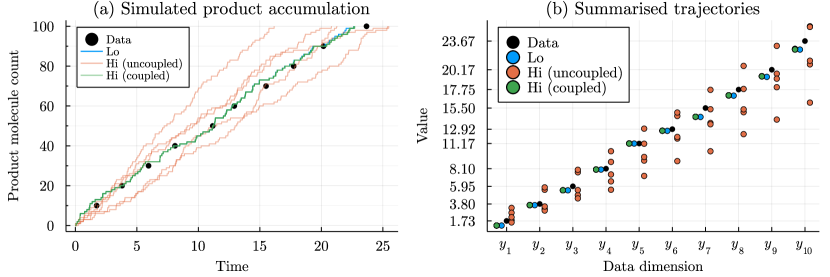
Figure 1: Effect of multifidelity coupling. (a) Example stochastic trajectories from the high and low-fidelity enzyme kinetics models in Equations 21 and 22 for parameters $\theta=(k_{1},k_{-1},k_{2})=(50,50,1)$, compared with data used for inference. For one low-fidelity simulation, we generate five uncoupled simulations and five coupled simulations. (b) Ten-dimensional data summarising simulated trajectories in (a). Black represents observed data, $y_{0}$; the single low-fidelity simulation $y_{\mathrm{lo}}\sim f_{\mathrm{lo}}(\cdot\mid\theta)$ is in blue; five uncoupled simulations $y_{\mathrm{hi}}\sim f_{\mathrm{hi}}(\cdot\mid\theta)$ are in orange; five coupled simulations $y_{\mathrm{hi}}\sim f_{\mathrm{hi}}(\cdot\mid\theta,y_{\mathrm{lo}})$ are in green (almost coincident).

We implement Algorithm 3 by setting a burn-in period of $N_{0}=10,000$, for which we generate $m_{i}\sim M=\mathrm{Poi}(1)$ high-fidelity simulations at each iteration, $i\leq N_{0}$. Once the burn-in period is complete, we define the partition $\mathcal{D}$ by learning a decision tree through a simple regression, as described in Section 4. For iterations $i>N_{0}$ beyond the burn-in period, we set a step size of $\delta=10^{3}$ for the gradient descent update in Equation 17.

5.1.3 Results

Algorithm 1 was run four times, setting the stop condition to $i=10,000$, $i=20,000$, $i=40,000$ and $i=80,000$. Similarly, Algorithm 3 was run five times, setting the stop condition to $i=40,000$, $i=80,000$, $i=160,000$, $i=320,000$ and $i=640,000$. Figure 2a shows how the variance in the estimate, $\hat{G}$, varies with the total simulation cost, $C_{\mathrm{tot}}$, shown for each of the two algorithms. The slope of each curve (on a log-log scale) is approximately $-1$, corresponding to the dominant behaviour of the MSE being reciprocal with total simulation time, as observed in Equation 11. The offset in the two curves corresponds to the inequality $\mathcal{J}_{\mathrm{mf}}<\mathcal{J}_{\mathrm{hi}}$ in the leading order coefficient, thereby demonstrating the improved performance of Algorithm 3 over Algorithm 1.

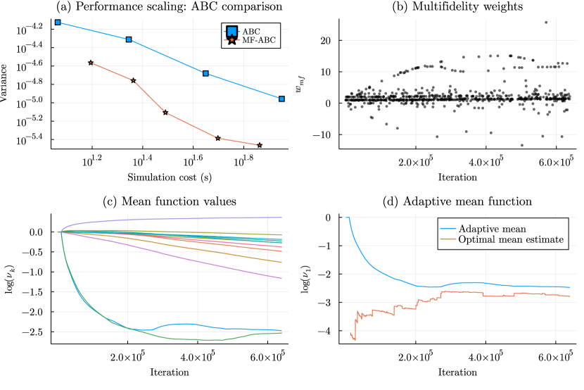
Figure 2: Multifidelity ABC. (a) Total simulation cost versus estimated variance of output estimate, $\hat{G}$, for four runs of Algorithm 1 (ABC) and five runs of Algorithm 3 (MF-ABC). (b) Values of the multifidelity weight, $w_{\mathrm{mf}}$, during the longest run of Algorithm 3, for iterations where $\omega_{\mathrm{mf}}\neq\omega_{\mathrm{lo}}$, such that the low-fidelity likelihood-free weighting is corrected based on at least one high-fidelity simulation. (c) The evolution of the values of $\nu_{k}^{(i)}$ during the longest run of Algorithm 3. (d) A comparison of the adaptive $\nu_{1}^{(i)}$ to the evolving best estimate of the optimal $\nu_{1}^{\star}$, given by Equation 16, based on the Monte Carlo estimates in Equation 18.

The values in Figure 2b show the multifidelity weights, $w_{i}$. We show only those weights not equal to zero or one, corresponding to those iterations where $\omega_{\mathrm{lo}}(\theta_{i},y_{\mathrm{lo},i})$ has been corrected by at least one $\omega_{\mathrm{hi}}(\theta_{i},y_{\mathrm{hi},i,j})\neq\omega_{\mathrm{lo}}(\theta_{i},y_{\mathrm{lo},i})$. Clearly there is a significant amount of correction applied to the low-fidelity weights. However, as demonstrated by the improved performance statistics, Algorithm 3 has learned the required allocation of computational budget to the high-fidelity simulations that balances the trade-off between achieving reduced overall simulation times and correcting inaccuracies in the low-fidelity simulation.

Each run of Algorithm 3 includes a burn-in period of $10,000$ iterations, at the conclusion of which a partition $\mathcal{D}$ is created, based on decision tree regression. In Appendix B, we show how this decision tree is used to define a piecewise-constant mean function, specifically for the partition $\mathcal{D}$ used for the final run of Algorithm 3 (i.e. for stopping condition $i=640,000$). In Figure 2c, we show the evolution of the values of $\nu_{k}^{(i)}$ used in this mean function, over iterations $i$. Following the updating rule in Equation 19, the trajectory of $\nu_{k}^{(i)}$ converges exponentially towards a Monte Carlo estimate of the optimal value $\nu_{k}^{\star}$ given in Equation 16. However, we can see from Figure 2c that, as more simulations are completed and the Monte Carlo estimates in Equation 18 evolve, the values of each parameter, $\nu_{k}$, track updated estimates. This is illustrated in Figure 2d for $\nu_{1}$, where the estimated optimum $\nu_{1}^{\star}$ evolves as more simulations are completed. We note that the gradient descent update in Equation 19 at iteration $i$ depends on all $\nu_{k}^{(i)}$ values. Thus, the observed convergence of $\nu_{1}^{(i)}$ to the evolving estimate of $\nu_{1}^{\star}$ is not necessarily monotonic.

Figure 2d illustrates the motivation for the use of gradient descent rather than simply using the analytically obtained optimum. When very few simulations have been completed, then the estimates in Equation 18 are small and their ratios are numerically unstable, and often far from the true optimum. If $\nu_{k}^{(i)}$ values are too small in early iterations, then estimates become more numerically unstable, since fewer high-fidelity simulations are completed for small $\mu$. Instead, using gradient descent ensures that enough high-fidelity simulations are completed for each $\mathcal{D}_{k}$, including those with low volume under the measure $\rho$, to stabilise the estimates in Equation 18 and thus stabilise the multifidelity algorithm.

5.2 Multifidelity Bayesian synthetic likelihood

Consider the same model of enzyme kinetics as in Section 5.1. As depicted in Figure 1, this model has low-fidelity (Michaelis–Menten) stochastic dynamics with distribution $f_{\mathrm{lo}}(\cdot\mid\theta)$, and coupled high-fidelity stochastic dynamics with distribution $f_{\mathrm{hi}}(\cdot\mid\theta,y_{\mathrm{lo}})$. We now redefine $\omega_{\mathrm{lo}}$ and $\omega_{\mathrm{hi}}$ to be Bayesian synthetic likelihoods, based on $K$ pairs of coupled simulations,

$$y_{\mathrm{lo},k} \sim f_{\mathrm{lo}}(\cdot\mid\theta),$$

$$y_{\mathrm{hi},k} \sim f_{\mathrm{hi}}(\cdot\mid\theta,y_{\mathrm{lo},k}),$$

for $k=1,\dots,K$. That is,

$$\omega_{\mathrm{lo}}(\theta,\mathbf{y}_{\mathrm{lo}}) =\mathcal{N}\left(y_{0}:\mu(\mathbf{y}_{\mathrm{lo}}),\Sigma(\mathbf{y}_{\mathrm{lo}})\right),$$

$$\omega_{\mathrm{hi}}(\theta,\mathbf{y}_{\mathrm{hi}}) =\mathcal{N}\left(y_{0}:\mu(\mathbf{y}_{\mathrm{hi}}),\Sigma(\mathbf{y}_{\mathrm{hi}})\right),$$

are the Gaussian likelihoods of the observed data, under the empirical mean and covariance of $K$ low-fidelity and (coupled) high-fidelity simulations, respectively.

Algorithm 1 was run three times, using $\omega_{\mathrm{hi}}(\theta,\mathbf{y}_{\mathrm{hi}})$ dependent on high-fidelity simulations $\mathbf{y}_{\mathrm{hi}}\sim f(\cdot\mid\theta)$, alone, and setting the stop condition to $i=2,500$, $i=5,000$ and $i=10,000$. Similarly, Algorithm 3 was run four times using the coupled multifidelity model, setting the stop condition to $i=4,000$, $i=8,000$, $i=16,000$ and $i=32,000$, and initialising with a burn-in of size $N_{0}=2,000$. The adaptive step size is set to $\delta=10^{8}$. In both algorithms, we set the number of simulations required for each evaluation of $\omega_{\mathrm{hi}}(\theta,(y_{\mathrm{hi},1},\dots,y_{\mathrm{hi},K}))$ or $\omega_{\mathrm{lo}}(\theta,(y_{\mathrm{lo},1},\dots,y_{\mathrm{lo},K}))$ as $K=100$.

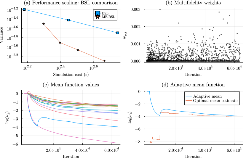
Figure 3: Multifidelity BSL. (a) Total simulation cost versus estimated variance of output estimate, $\hat{G}$, for three runs of Algorithm 1 (BSL) and four runs of Algorithm 3 (MF-BSL). (b) Values of the multifidelity weight, $w_{\mathrm{mf}}$, during the longest run of Algorithm 3, for iterations where $\omega_{\mathrm{mf}}\neq\omega_{\mathrm{lo}}$, such that the low-fidelity likelihood-free weighting is corrected based on at least one high-fidelity simulation. (c) The evolution of the values of $\nu_{k}^{(i)}$ during the longest run of Algorithm 3. (d) A comparison of the adaptive $\nu_{1}^{(i)}$ to the evolving best estimate of the optimal $\nu_{1}^{\star}$, given by Equation 16, based on the Monte Carlo estimates in Equation 18.

Figure 3 depicts the performance of multifidelity Bayesian synthetic likelihood (BSL) inference, where Algorithm 3 is applied with BSL likelihood-free weightings, $\omega_{\mathrm{lo}}$ and $\omega_{\mathrm{hi}}$. As with MF-ABC, Figure 3a shows that the MF-BSL generates improved performance over high-fidelity BSL inference, achieving lower variance estimates for a given computational budget. We also note in Figure 3a that the curve corresponding to MF-BSL has slope less than $-1$. This is due to (a) the overhead cost of the initial burn-in period of Algorithm 3, and also (b) the conservative convergence of $\nu^{(i)}$ to the optimum, as shown in Figure 3c–d. Both observations imply that earlier iterations are less efficiently produced than later iterations, meaning that larger samples show greater improvements than expected from the reciprocal relationship in Equation 11.

Comparing Figure 3b to Figure 2b, we note that there are very few negative multifidelity weightings in MF-BSL, in comparison to MF-ABC. We can conclude that the Bayesian synthetic likelihood, constructed using low-fidelity simulations, tends to underestimate the likelihood of the observed data compared to using high-fidelity simulations. We note also in this comparison that the multifidelity likelihood-free weightings are on significantly different scales.

6 Discussion

The characteristic computational burden of simulation-based, likelihood-free Bayesian inference methods is often a barrier to their successful implementation. Multifidelity simulation techniques have previously been shown to improve the efficiency of likelihood-free inference in the context of ABC. In this work, we have demonstrated that these techniques can be readily applied to general likelihood-free approaches. Furthermore, we have introduced a computational methodology for automating the multifidelity approach, adaptively allocating simulation resources across different fidelities in order to ensure near-optimal efficiency gains from this technique. As parameter space is explored, our methodology, given in Algorithm 3, learns the relationships between simulation accuracy and simulation costs at the different fidelities, and adapts the requirement for high-fidelity simulation accordingly.

The multifidelity approach to likelihood-free inference is one of a number of strategies for speeding up inference, which include MCMC and SMC sampling techniques [Marjoram et al., 2003, Sisson et al., 2007, Toni et al., 2009] and methods for variance reduction such as multilevel estimation [Giles, 2015, Guha and Tan, 2017, Warne et al., 2018, Jasra et al., 2019]. A key observation in the previous work of Prescott and Baker [2021] and Warne et al. [2021b] is that applying multifidelity techniques provides ‘orthogonal’ improvements that combine synergistically with these other established approaches to improving efficiency. Similarly, we envision that Algorithm 3 can be adapted into an SMC or multilevel algorithm with minimal difficulty, following the templates set by Prescott and Baker [2021] and Warne et al. [2021b].

The multifidelity approach discussed in this work is a highly flexible generalisation of existing multifidelity techniques, which can be viewed as special cases of Algorithm 2. In each of MF-ABC [Prescott and Baker, 2020, 2021], LZ-ABC [Prangle, 2016], and DA-ABC [Everitt and Rowińska, 2021], it is assumed that $\omega_{\mathrm{hi}}$ is an ABC likelihood-free weighting, which we relax in this work. Furthermore, LZ-ABC and DA-ABC both use $\omega_{\mathrm{lo}}\equiv 0$, so that parameters are always rejected if no high-fidelity simulation is completed. Clearly, we relax this assumption to allow for any low-fidelity likelihood-free weighting. In all of MF-ABC, LZ-ABC and DA-ABC, the conditional distribution of $M$, given a parameter value $\theta$ and low-fidelity simulation output $\mathbf{y}_{\mathrm{lo}}$ is Bernoulli distributed, with mean $\mu(\theta,\mathbf{y}_{\mathrm{lo}})\in(0,1]$. In this work we change this distribution to Poisson, to ease analytical results, but any conditional distribution for $M$ can be used. These adaptations are explored further in Appendix A.

In the case of MF-ABC (as originally formulated by Prescott and Baker [2020]) and DA-ABC [Christen and Fox, 2005, Everitt and Rowińska, 2021], the mean function, $\mu(\theta,y_{\mathrm{lo}})$, depends on a single low-fidelity simulation and is assumed to be piecewise constant in the value of the indicator function $\mathbf{1}(d(y_{\mathrm{lo}},y_{0})<\epsilon)$. LZ-ABC is more generic in its definition of $\mu=\mu(\phi(\theta,\mathbf{y}_{\mathrm{lo}}))$ to depend on the value of any decision statistic, $\phi$. In this work, we consider more general piecewise constant mean functions, $\mu_{\mathcal{D}}$, for heuristically derived partitions $\mathcal{D}$ of $(\theta,\mathbf{y}_{\mathrm{lo}})$-space. We observe that $(\theta,\mathbf{y}_{\mathrm{lo}})$ may be of very high dimension; in the BSL example in Section 5.2, having $K=100$ low-fidelity simulations $y_{\mathrm{lo}}\in\mathbb{R}^{10}$ means that the input to $\mu$ is of dimension $1003$. In this situation, it may be tempting to seek a mean function that only depends on $\theta$. However, we recall that the optimal mean function, $\mu^{\star}(\theta,\mathbf{y}_{\mathrm{lo}})$, derived in 6, depends on the conditional expectation $\mathbf{E}((\omega_{\mathrm{hi}}-\omega_{\mathrm{lo}})^{2}\mid\theta,\mathbf{y}_{\mathrm{lo}})$. Thus, by ignoring $\mathbf{y}_{\mathrm{lo}}$, we would ignore the information about $\omega_{\mathrm{hi}}$ given by the evaluation of $\omega_{\mathrm{lo}}(\theta,\mathbf{y}_{\mathrm{lo}})$. Furthermore, the high dimension of the inputs to $\mu^{\star}$ suggest that this function is not necessarily well-approximated by a decision tree. Future work may focus on methods to learn the optimal mean function directly without resorting to piecewise constant approximations [Levine and Stuart, 2021]. The key problem is ensuring the conservatism of any alternative estimate of $\mu^{\star}$, recalling that the variance of $w_{\mathrm{mf}}$ is inversely proportional to $\mu$.

In the example explored in Section 5, we considered the use of Algorithm 3 where $\omega_{\mathrm{hi}}$ and $\omega_{\mathrm{lo}}$ were first both ABC likelihood-free weightings, and then both BSL likelihood-free weightings. In principle, this method should also allow for $\omega_{\mathrm{lo}}$ to be, for example, an ABC likelihood-free weighting based on a single low-fidelity simulation, and $\omega_{\mathrm{hi}}$ to be a BSL likelihood-free weighting based on $K>1$ high-fidelity simulations. However, the success of the multifidelity method depends explicitly on the function $\eta(\theta,\mathbf{y}_{\mathrm{lo}})=\mathbf{E}((\omega_{\mathrm{hi}}-\omega_{\mathrm{lo}})^{2}\mid\theta,\mathbf{y}_{\mathrm{lo}})$ being sufficiently small, as quantified in 7. If $\omega_{\mathrm{lo}}$ and $\omega_{\mathrm{hi}}$ are on different scales, as is likely when one is an ABC weighting and one a BSL weighting, then this function is not sufficiently small in general, and so the multifidelity approach fails. We note, however, that we could instead consider the scaled low-fidelity weighting, $\tilde{\omega}_{\mathrm{lo}}=\gamma\mathbf{\omega}_{\mathrm{lo}}$, in place of $\omega_{\mathrm{lo}}$ in Algorithms 2 and 3 with no change to the target distribution. Here, $\gamma$ is an additional parameter that can be tuned with $\mu$ when minimising the performance metric, $\mathcal{J}_{\mathrm{mf}}$; the optimal value of this parameter would need to be learned in parallel with the optimal mean function, $\mu$. We defer this adaptation to future work.

Finally, this work follows Prescott and Baker [2020, 2021] in considering only a single low-fidelity model. There is significant scope for further improvements by applying these approaches to suites of low-fidelity approximations [Gorodetsky et al., 2021]. For example, exact stochastic simulations of biochemical networks, such as that simulated in Section 5, may also be approximated by tau-leaping [Gillespie, 2001, Warne et al., 2019], where the time discretisation parameter $\tau$ tends to be chosen to trade off computational savings against accuracy: exactly the trade-off explored in this work. Clearly, this parameter therefore has important consequences for the success of a multifidelity inference approach using such an approximation strategy. More generally, a full exploration of the use of multiple low-fidelity model approximations will be vital for the full potential of multifidelity likelihood-free inference to be realised.

Acknowledgements

REB and TPP acknowledge funding for this work through the BBSRC/UKRI grant BB/R00816/1. TPP is supported by the Alan Turing Institute and by Wave 1 of the UKRI Strategic Priorities Fund, under the “Shocks and Resilience” theme of the EPSRC/UKRI grant EP/W006022/1. DJW thanks the Australian Mathematical Society for the Lift-off Fellowship, and acknowledges continued support from the Centre for Data Science at QUT and the ARC Centre of Excellence in Mathematical and Statistical Frontiers (ACEMS; CE140100049). REB is supported by a Royal Society Wolfson Research Merit Award.

Appendix A Analytical results: Comparing performance

A.1 5

Proof.

The leading order performance of each of Algorithm 1 and Algorithm 2 is given in terms of increasing computational budget, $C_{\mathrm{tot}}$, in Equation 10 and Equation 11, respectively. For the performance of Algorithm 2 to exceed that of Algorithm 1, we compare the leading order coefficients from Equations 10 and 11, requiring

$$\frac{\mathbf{E}(C_{\mathrm{mf}})\mathbf{E}(w_{\mathrm{mf}}^{2}\Delta^{2})}{\mathbf{E}(w_{\mathrm{mf}})^{2}}<\frac{\mathbf{E}(C_{\mathrm{hi}})\mathbf{E}(w_{\mathrm{hi}}^{2}\Delta^{2})}{\mathbf{E}(w_{\mathrm{hi}})^{2}}.$$ (23)

We note that $\mathbf{E}(w_{\mathrm{mf}}\mid\theta)=\pi(\theta)L_{\mathrm{mf}}(\theta)/q(\theta)$ and $\mathbf{E}(w_{\mathrm{hi}}\mid\theta)=\pi(\theta)L_{\mathrm{hi}}(\theta)/q(\theta)$. Since $L_{\mathrm{mf}}=L_{\mathrm{hi}}$, as shown in 4, the denominators in Equation 23 are therefore equal. Thus,

$$\mathcal{J}_{\mathrm{mf}}=\mathbf{E}(C_{\mathrm{mf}})\mathbf{E}(w_{\mathrm{mf}}^{2}\Delta^{2})<\mathbf{E}(C_{\mathrm{hi}})\mathbf{E}(w_{\mathrm{hi}}^{2}\Delta^{2})=\mathcal{J}_{\mathrm{hi}},$$

is the condition for Algorithm 2 to outperform Algorithm 1.

Taking the right-hand side of this inequality first, clearly the expected simulation time is $\mathbf{E}(C_{\mathrm{hi}})=\bar{c}_{\mathrm{hi}}$, for the constant $\bar{c}_{\mathrm{hi}}$ defined in Equation 12c. Similarly, we can write

$$\mathbf{E}(w_{\mathrm{hi}}^{2}\Delta^{2})=\int\left(\frac{\pi(\theta)}{q(\theta)}\Delta(\theta)\right)^{2}\left[\int\omega_{\mathrm{hi}}(\theta,\mathbf{y}_{\mathrm{hi}})^{2}f_{\mathrm{hi}}(\mathbf{y}_{\mathrm{hi}}\mid\theta)\mathrm{d}\mathbf{y}_{\mathrm{hi}}\right]q(\theta)\mathrm{d}\theta=V_{\mathrm{hi}},$$

as given in Equation 12d. Thus, $\mathcal{J}_{\mathrm{hi}}=\bar{c}_{\mathrm{hi}}V_{\mathrm{hi}}$.

For the left-hand side of the performance inequality, we take each expectation in $\mathcal{J}_{\mathrm{mf}}$ in turn. We first note that the expected iteration cost of Algorithm 2, $\mathbf{E}(C_{\mathrm{mf}})$, is the sum of the expected cost of a single low-fidelity simulation, and the expected cost of $M$ high-fidelity simulations. By definition, the expected cost of a single low-fidelity simulation $\mathbf{y}_{\mathrm{lo}}\sim f_{\mathrm{lo}}(\cdot\mid\theta)$ across $\theta\sim q(\cdot)$ is given by $\bar{c}_{\mathrm{lo}}$. Thus the remaining cost, $\mathbf{E}(\delta C_{\mathrm{mf}})=\mathbf{E}(C_{\mathrm{mf}})-\bar{c}_{\mathrm{lo}}$, is the expected cost of $M$ high-fidelity simulations. Conditioning on $\theta$, $\mathbf{y}_{\mathrm{lo}}$ and $M=m$, the expected remaining cost is, by definition,

$$\mathbf{E}(\delta C_{\mathrm{mf}}\mid\theta,\mathbf{y}_{\mathrm{lo}},M=m)=mc_{\mathrm{hi}}(\theta,\mathbf{y}_{\mathrm{lo}}).$$

Taking expectations over the conditional distribution $M\sim\mathrm{Poi}(\mu(\theta,\mathbf{y}_{\mathrm{lo}}))$, we have

$$\mathbf{E}(\delta C_{\mathrm{mf}}\mid\theta,\mathbf{y}_{\mathrm{lo}})=\mu(\theta,\mathbf{y}_{\mathrm{lo}})c_{\mathrm{hi}}(\theta,\mathbf{y}_{\mathrm{lo}}).$$

Finally, integrating this expression over the density $\rho$ in Equation 12j gives the first factor of Equation 12b.

It remains to show that

$$\mathbf{E}(w_{\mathrm{mf}}^{2}\Delta^{2})=V_{\mathrm{mf}}+\iint\Delta_{q}(\theta)^{2}\frac{\eta(\theta,\mathbf{y}_{\mathrm{lo}})}{\mu(\theta,\mathbf{y}_{\mathrm{lo}})}\leavevmode\nobreak\ \rho(\theta,\mathbf{y}_{\mathrm{lo}})\mathrm{d}\theta\mathrm{d}\mathbf{y}_{\mathrm{lo}}.$$

We first condition on $\theta$, $\mathbf{y}_{\mathrm{lo}}$ and $M=m$, to write

$$\mathbf{E}(w_{\mathrm{mf}}^{2}\Delta^{2}\mid\theta,\mathbf{y}_{\mathrm{lo}},m) =\Delta_{q}^{2}\mathbf{E}(\omega_{\mathrm{mf}}^{2}\mid\theta,\mathbf{y}_{\mathrm{lo}},m)$$

$$=\Delta_{q}^{2}\left[\omega_{\mathrm{lo}}^{2}+\frac{2}{\mu}\omega_{\mathrm{lo}}\mathbf{E}\left(D_{m}\mid\theta,\mathbf{y}_{\mathrm{lo}}\right)+\frac{1}{\mu^{2}}\mathbf{E}\left(D_{m}^{2}\mid\theta,\mathbf{y}_{\mathrm{lo}}\right)\right],$$

for the random variable $D_{m}=\sum_{i=1}^{m}\left(\omega_{\mathrm{hi},i}-\omega_{\mathrm{lo}}\right)$. It is straightforward to show that

$$\mathbf{E}(D_{m}\mid\theta,\mathbf{y}_{\mathrm{lo}}) =m\mathbf{E}(\omega_{\mathrm{hi}}\mid\theta,\mathbf{y}_{\mathrm{lo}})-m\omega_{\mathrm{lo}},$$

$$\mathbf{E}(D_{m}^{2}\mid\theta,\mathbf{y}_{\mathrm{lo}}) =m\mathbf{E}\left((\omega_{\mathrm{hi}}-\omega_{\mathrm{lo}})^{2}\mid\theta,\mathbf{y}_{\mathrm{lo}}\right)+(m^{2}-m)\mathbf{E}(\omega_{\mathrm{hi}}-\omega_{\mathrm{lo}}\mid\theta,\mathbf{y}_{\mathrm{lo}})^{2},$$

where we exploit the conditional independence of the high-fidelity simulations $\mathbf{y}_{\mathrm{hi},i}$ and $\mathbf{y}_{\mathrm{hi},j}$, for $i\neq j$. On substitution of these conditional expectations, we then rearrange to write

$$\mathbf{E}(w_{\mathrm{mf}}^{2}\Delta^{2}\mid\theta,\mathbf{y}_{\mathrm{lo}},m)=\Delta_{q}^{2}\left[\left(1-\frac{2m}{\mu}\right)\omega_{\mathrm{lo}}^{2}+\frac{2m}{\mu}\omega_{\mathrm{lo}}\lambda_{\mathrm{hi}}+\frac{m}{\mu^{2}}\mathrm{Var}(\omega_{\mathrm{hi}}-\omega_{\mathrm{lo}}\mid\theta,\mathbf{y}_{\mathrm{lo}})+\left(\frac{m(\lambda_{\mathrm{hi}}-\omega_{\mathrm{lo}})}{\mu}\right)^{2}\right],$$

where we write the conditional expectation $\lambda_{\mathrm{hi}}(\theta,\mathbf{y}_{\mathrm{lo}})=\mathbf{E}(\omega_{\mathrm{hi}}\mid\theta,\mathbf{y}_{\mathrm{lo}})$. At this point we can take expectations over $M$ and rearrange to give

$$\mathbf{E}(w_{\mathrm{mf}}^{2}\Delta^{2}\mid\theta,\mathbf{y}_{\mathrm{lo}}) =\Delta_{q}^{2}\left[2\omega_{\mathrm{lo}}\lambda_{\mathrm{hi}}-\omega_{\mathrm{lo}}^{2}+\frac{1}{\mu}\mathrm{Var}(\omega_{\mathrm{hi}}-\omega_{\mathrm{lo}}\mid\theta,\mathbf{y}_{\mathrm{lo}})+\frac{(\mathrm{Var}(M\mid\theta,\mathbf{y}_{\mathrm{lo}})+\mu^{2})(\lambda_{\mathrm{hi}}-\omega_{\mathrm{lo}})^{2}}{\mu^{2}}\right]$$

$$=\Delta_{q}^{2}\left[\lambda_{\mathrm{hi}}^{2}+\frac{1}{\mu}\left(\mathrm{Var}(\omega_{\mathrm{hi}}-\omega_{\mathrm{lo}}\mid\theta,\mathbf{y}_{\mathrm{lo}})+\frac{\mathrm{Var}(M\mid\theta,\mathbf{y}_{\mathrm{lo}})}{\mu}\left(\mathbf{E}(\omega_{\mathrm{hi}}-\omega_{\mathrm{lo}}\mid\theta,\mathbf{y}_{\mathrm{lo}})\right)^{2}\right)\right].$$ (24)

Here, we can use the assumption that $M$ conditioned on $\theta$ and $\mathbf{y}_{\mathrm{lo}}$ is Poisson distributed, noting that the statement of 5 can be adapted for other conditional distributions of $M$ with different conditional variance functions. Under the Poisson assumption, we can substitute $\mathrm{Var}(M\mid\theta,\mathbf{y}_{\mathrm{lo}})=\mu(\theta,\mathbf{y}_{\mathrm{lo}})$ to give

$$\mathbf{E}(w_{\mathrm{mf}}^{2}\Delta^{2}\mid\theta,\mathbf{y}_{\mathrm{lo}})=\Delta_{q}^{2}\left[\lambda_{\mathrm{hi}}^{2}+\frac{\mathbf{E}\left(\left(\omega_{\mathrm{hi}}-\omega_{\mathrm{lo}}\right)^{2}\mid\theta,\mathbf{y}_{\mathrm{lo}}\right)}{\mu(\theta,\mathbf{y}_{\mathrm{lo}})}\right].$$

Finally, we take expectations with respect to the probability density $\rho$ in Equation 12j, and the product in Equation 12b follows. ∎

A.1.1 Alternative conditional distributions for $M$

The proof above derives the performance measure $\mathcal{J}_{\mathrm{mf}}$ given in Equation 12b, under the assumption that the conditional distribution of $M$, given $\theta$ and $\mathbf{y}_{\mathrm{lo}}$, is Poisson with mean $\mu(\theta,\mathbf{y}_{\mathrm{lo}})$. The following corollaries adapt the expression for $\mathcal{J}_{\mathrm{mf}}$ in the case of alternative conditional distributions for $M$. We first define the MSE,

$$E_{\mathrm{mf}}=\iint\left[\lambda_{\mathrm{hi}}(\theta,\mathbf{y}_{\mathrm{lo}})-\omega_{\mathrm{lo}}(\theta,\mathbf{y}_{\mathrm{lo}})\right]^{2}\leavevmode\nobreak\ \rho(\theta,\mathbf{y}_{\mathrm{lo}})\mathrm{d}\theta\mathrm{d}\mathbf{y}_{\mathrm{lo}},$$

between $\omega_{\mathrm{lo}}(\theta,\mathbf{y}_{\mathrm{lo}})$ and $\lambda_{\mathrm{hi}}(\theta,\mathbf{y}_{\mathrm{lo}})=\mathbf{E}(\omega_{\mathrm{hi}}\mid\theta,\mathbf{y}_{\mathrm{lo}})$.

Corollary 10.

If $M\sim\mathrm{Bin}(M_{\max},p(\theta,\mathbf{y}_{\mathrm{lo}}))$ is binomially distributed with maximum value $M_{\max}$ and mean $\mu(\theta,\mathbf{y}_{\mathrm{lo}})$, where $p=\mu/M_{\max}$, then

$$\mathcal{J}_{\mathrm{mf}}[\mu] =\left(\bar{c}_{\mathrm{lo}}+\iint\mu(\theta,\mathbf{y}_{\mathrm{lo}})c_{\mathrm{hi}}(\theta,\mathbf{y}_{\mathrm{lo}})\leavevmode\nobreak\ \rho(\theta,\mathbf{y}_{\mathrm{lo}})\mathrm{d}\theta\mathrm{d}\mathbf{y}_{\mathrm{lo}}\right)$$

$$\quad{}\times\left(V_{\mathrm{mf}}-\frac{E_{\mathrm{mf}}}{M_{\max}}+\iint\Delta_{q}(\theta)^{2}\frac{\eta(\theta,\mathbf{y}_{\mathrm{lo}})}{\mu(\theta,\mathbf{y}_{\mathrm{lo}})}\leavevmode\nobreak\ \rho(\theta,\mathbf{y}_{\mathrm{lo}})\mathrm{d}\theta\mathrm{d}\mathbf{y}_{\mathrm{lo}}\right).$$ (25)

Proof.

We substitute $\mathrm{Var}(M\mid\theta,\mathbf{y}_{\mathrm{lo}})=\mu\left(1-\mu/M_{\max}\right)$ into Equation 24, and the result follows. ∎

We note in the result above that for $\mu$ to be the conditional mean of $M\sim\mathrm{Bin}(M_{\max},p(\theta,\mathbf{y}_{\mathrm{lo}}))$, we must constrain the values of $\mu$ such that $\mu(\theta,\mathbf{y}_{\mathrm{lo}})\in(0,M_{\max}]$. This constraint alters the derivation of the optimal $\mu^{\star}$, in the case of a binomial conditional distribution with fixed $M_{\max}$.

Corollary 11.

If $M\sim\mathrm{Geo}(p(\theta,\mathbf{y}_{\mathrm{lo}}))$ is geometrically distributed on the non-negative integers, with mean $\mu(\theta,\mathbf{y}_{\mathrm{lo}})$, where $p=1/(1+\mu)$, then

$$\mathcal{J}_{\mathrm{mf}}[\mu] =\left(\bar{c}_{\mathrm{lo}}+\iint\mu(\theta,\mathbf{y}_{\mathrm{lo}})c_{\mathrm{hi}}(\theta,\mathbf{y}_{\mathrm{lo}})\leavevmode\nobreak\ \rho(\theta,\mathbf{y}_{\mathrm{lo}})\mathrm{d}\theta\mathrm{d}\mathbf{y}_{\mathrm{lo}}\right)$$

$$\quad{}\times\left(V_{\mathrm{mf}}+E_{\mathrm{mf}}+\iint\Delta_{q}(\theta)^{2}\frac{\eta(\theta,\mathbf{y}_{\mathrm{lo}})}{\mu(\theta,\mathbf{y}_{\mathrm{lo}})}\leavevmode\nobreak\ \rho(\theta,\mathbf{y}_{\mathrm{lo}})\mathrm{d}\theta\mathrm{d}\mathbf{y}_{\mathrm{lo}}\right).$$ (26a)

Proof.

We substitute $\mathrm{Var}(M\mid\theta,\mathbf{y}_{\mathrm{lo}})=\mu\left(1+\mu\right)$ into Equation 24, and the result follows. ∎

A.2 6

We return to the assumption that $M$ is conditionally Poisson distributed, given $\theta$ and $\mathbf{y}_{\mathrm{lo}}$.

Proof.

We write the functional $\mathcal{J}_{\mathrm{mf}}[\mu]=\mathcal{C}[\mu]\mathcal{V}[\mu]$ in Equation 12b as the product of functionals,

$$\mathcal{C}[\mu] =\bar{c}_{\mathrm{lo}}+\iint\mu c_{\mathrm{hi}}\leavevmode\nobreak\ \rho\mathrm{d}\theta\mathrm{d}\mathbf{y}_{\mathrm{lo}},$$ (27a)

$$\mathcal{V}[\mu] =V_{\mathrm{mf}}+\iint\Delta_{q}^{2}\frac{\eta}{\mu}\leavevmode\nobreak\ \rho\mathrm{d}\theta\mathrm{d}\mathbf{y}_{\mathrm{lo}}.$$ (27b)

Standard ‘product rule’ results from calculus of variations allows us to write the functional derivative of $\mathcal{J}_{\mathrm{mf}}$ with respect to $\mu$ as

$$\frac{\delta\mathcal{J}_{\mathrm{mf}}}{\delta\mu} =\mathcal{V}[\mu]\frac{\delta\mathcal{C}}{\delta\mu}+\mathcal{C}[\mu]\frac{\delta\mathcal{V}}{\delta\mu}$$

$$=\mathcal{V}[\mu]c_{\mathrm{hi}}\rho-\mathcal{C}[\mu]\frac{\Delta_{q}^{2}\eta\rho}{\mu^{2}}.$$

Setting this functional derivative to zero, the optimal function, $\mu^{\star}$, satisfies

$$\mu^{\star}(\theta,\mathbf{y}_{\mathrm{lo}})^{2}=\frac{\mathcal{C}[\mu^{\star}]}{\mathcal{V}[\mu^{\star}]}\frac{\Delta_{q}(\theta)^{2}\eta(\theta,\mathbf{y}_{\mathrm{lo}})}{c_{\mathrm{hi}}(\theta,\mathbf{y}_{\mathrm{lo}})}.$$ (28)

The result in Equation 13 follows on showing that $C[\mu^{\star}]/V[\mu^{\star}]=\bar{c}_{\mathrm{lo}}/V_{\mathrm{mf}}$.

On substituting Equation 28 into Equation 27 we find

$$\mathcal{C}[\mu^{\star}] =\bar{c}_{\mathrm{lo}}+\sqrt{\frac{\mathcal{C}[\mu^{\star}]}{\mathcal{V}[\mu^{\star}]}}\iint\sqrt{\Delta_{q}^{2}\eta c_{\mathrm{hi}}}\leavevmode\nobreak\ \rho\mathrm{d}\theta\mathrm{d}\mathbf{y}_{\mathrm{lo}},$$

$$\mathcal{V}[\mu^{\star}] =V_{\mathrm{mf}}+\sqrt{\frac{\mathcal{V}[\mu^{\star}]}{\mathcal{C}[\mu^{\star}]}}\iint\sqrt{\Delta_{q}^{2}\eta c_{\mathrm{hi}}}\leavevmode\nobreak\ \rho\mathrm{d}\theta\mathrm{d}\mathbf{y}_{\mathrm{lo}},$$

from which it follows that

$$\sqrt{\frac{\mathcal{V}[\mu^{\star}]}{\mathcal{C}[\mu^{\star}]}}\bar{c}_{\mathrm{lo}}=\sqrt{\frac{\mathcal{C}[\mu^{\star}]}{\mathcal{V}[\mu^{\star}]}}V_{\mathrm{mf}}=\sqrt{\mathcal{C}[\mu^{\star}]\mathcal{V}[\mu^{\star}]}-\iint\sqrt{\Delta_{q}^{2}\eta c_{\mathrm{hi}}}\leavevmode\nobreak\ \rho\mathrm{d}\theta\mathrm{d}\mathbf{y}_{\mathrm{lo}}.$$

Multiplying this equation by $\sqrt{\mathcal{C}[\mu^{\star}]\mathcal{V}[\mu^{\star}]}$, we have $\mathcal{V}[\mu^{\star}]\bar{c}_{\mathrm{lo}}=\mathcal{C}[\mu^{\star}]V_{\mathrm{mf}}$, and thus Equation 13 follows from Equation 28. ∎

A.3 7

Proof.

On substituting Equation 13 into Equation 27, we find that the condition $\mathcal{J}_{\mathrm{mf}}^{\star}=\mathcal{J}_{\mathrm{mf}}[\mu^{\star}]<\mathcal{J}_{\mathrm{hi}}=\bar{c}_{\mathrm{hi}}V_{\mathrm{hi}}$ is equivalent to

$$\left(\sqrt{\bar{c}_{\mathrm{lo}}V_{\mathrm{mf}}}+\iint\sqrt{\Delta_{q}(\theta)^{2}\eta(\theta,\mathbf{y}_{\mathrm{lo}})c_{\mathrm{hi}}(\theta,\mathbf{y}_{\mathrm{lo}})}\leavevmode\nobreak\ \rho(\theta,\mathbf{y}_{\mathrm{lo}})\mathrm{d}\theta\mathrm{d}\mathbf{y}_{\mathrm{lo}}\right)^{2}<\bar{c}_{\mathrm{hi}}V_{\mathrm{hi}}.$$

A simple rearrangement of this inequality gives the inequality in Equation 14. ∎

To interpret the condition

$$\sqrt{\frac{\bar{c}_{\mathrm{lo}}}{\bar{c}_{\mathrm{hi}}}\frac{V_{\mathrm{mf}}}{V_{\mathrm{hi}}}}+\iint\sqrt{\frac{\Delta_{q}(\theta)^{2}\eta(\theta,\mathbf{y}_{\mathrm{lo}})}{V_{\mathrm{hi}}}}\sqrt{\frac{c_{\mathrm{hi}}(\theta,\mathbf{y}_{\mathrm{lo}})}{\bar{c}_{\mathrm{hi}}}}\leavevmode\nobreak\ \rho(\theta,\mathbf{y}_{\mathrm{lo}})\mathrm{d}\theta\mathrm{d}\mathbf{y}_{\mathrm{lo}}<1$$

in Equation 14, we note that the first term is determined by (a) our assumption of a significant reduction in simulation burden of the low-fidelity model over the high-fidelity model, $\bar{c}_{\mathrm{lo}}<\bar{c}_{\mathrm{hi}}$, and (b) the ratio of the two integrals,

$$\frac{V_{\mathrm{mf}}}{V_{\mathrm{hi}}}=\frac{\int\Delta_{q}(\theta)^{2}\mathbf{E}(\mathbf{E}(\omega_{\mathrm{hi}}\mid\theta,\mathbf{y}_{\mathrm{lo}})^{2}\mid\theta)q(\theta)\leavevmode\nobreak\ \mathrm{d}\theta}{\int\Delta_{q}(\theta)^{2}\mathbf{E}(\omega_{\mathrm{hi}}^{2}\mid\theta)q(\theta)\leavevmode\nobreak\ \mathrm{d}\theta}.$$

Exploiting the law of total variance, we note that

$$\mathbf{E}(\omega_{\mathrm{hi}}^{2}\mid\theta) =\mathrm{Var}(\omega_{\mathrm{hi}}\mid\theta)+L_{\mathrm{hi}}(\theta)^{2},$$

$$\mathbf{E}(\mathbf{E}(\omega_{\mathrm{hi}}\mid\theta,\mathbf{y}_{\mathrm{lo}})^{2}\mid\theta) =\mathrm{Var}(\mathbf{E}(\omega_{\mathrm{hi}}\mid\theta,\mathbf{y}_{\mathrm{lo}})\mid\theta)+L_{\mathrm{hi}}(\theta)^{2}$$

$$=\mathbf{E}(\omega_{\mathrm{hi}}^{2}\mid\theta)-\mathbf{E}(\mathrm{Var}(\omega_{\mathrm{hi}}\mid\theta,\mathbf{y}_{\mathrm{lo}})\mid\theta).$$

These equalities imply that

$$\mathbf{E}(\omega_{\mathrm{hi}}\mid\theta)^{2}\leq\mathbf{E}(\mathbf{E}(\omega_{\mathrm{hi}}\mid\theta,\mathbf{y}_{\mathrm{lo}})^{2}\mid\theta)\leq\mathbf{E}(\omega_{\mathrm{hi}}^{2}\mid\theta),$$

where the lower bound is achieved for $\mathbf{y}_{\mathrm{hi}}$ independent of $\mathbf{y}_{\mathrm{lo}}$, while the upper bound would be achieved if $\mathbf{y}_{\mathrm{hi}}$ were a deterministic function of $\mathbf{y}_{\mathrm{lo}}$. In particular, $V_{\mathrm{mf}}/V_{\mathrm{hi}}\leq 1$, and so the first term of Equation 14 is small whenever the low-fidelity model provides significant computational savings versus the high-fidelity model.

The second term in Equation 14 quantifies the detriment to the performance of Algorithm 2 that arises from the inaccuracy of $\omega_{\mathrm{lo}}$ as an estimate of $\omega_{\mathrm{hi}}$. The function $\eta(\theta,\mathbf{y}_{\mathrm{lo}})=\mathbf{E}((\omega_{\mathrm{hi}}-\omega_{\mathrm{lo}})^{2}\mid\theta,\mathbf{y}_{\mathrm{lo}})$ is integrated across the density $\rho$, weighted by the relative computational cost of the high-fidelity simulation, $c_{\mathrm{hi}}(\theta,\mathbf{y}_{\mathrm{lo}})/\bar{c}_{\mathrm{hi}}$, and by the contribution of $G(\theta)$ to the variance of the estimated posterior expectation of $G$. We can conclude that the multifidelity approach requires that the low-fidelity model is accurate in the regions of parameter space where high-fidelity simulations are particularly expensive.

To summarise: if (a) the ratio between average low-fidelity simulation costs and high-fidelity simulation costs is suitably small, and (b) the average disagreement between likelihood-free weightings, as measured by $\eta$, is suitably small, then Equation 14 will be satisfied and thus a mean function, $\mu^{\star}$, exists such that Algorithm 2 is more efficient than Algorithm 1.

Appendix B Mean functions

Algorithm 4 Piecewise constant mean function $\mu_{\mathcal{D}}(\theta,y_{\mathrm{lo}};\nu)$ used in MF-ABC Algorithm 3, depicted in Figure 2c, at final iteration.

$\theta=(k_{1},k_{-1},k_{2})$; $y_{\mathrm{lo}}=(y_{1},y_{2},\dots,y_{10})$.

if $y_{7}\leq 13.867$ then

     return $\nu_{1}=0.084$.

else

     if $k_{2}\leq 1.14$  then

         if $y_{8}\leq 16.219$ then

              return $\nu_{2}=0.616$.

         else

              if $k_{2}\leq 0.88$  then

                  return $\nu_{3}=0.08$.

              else

                  if $y_{10}\leq 26.208$ then

                       if $k_{1}\leq 91.265$  then

                           return $\nu_{4}=0.313$.

                       else

                           return $\nu_{5}=0.76$.                        

                  else

                       if $y_{7}\leq 15.151$ then

                           return $\nu_{6}=0.761$.

                       else

                           if $y_{1}\leq 3.371$ then

                                if $y_{5}\leq 11.264$ then

                                    return $\nu_{7}=0.688$.

                                else

                                    return $\nu_{8}=0.467$.                                 

                           else

                                return $\nu_{9}=0.797$.                                                                                            

     else

         if $y_{10}\leq 26.136$ then

              if $y_{7}\leq 14.17$ then

                  return $\nu_{10}=0.929$.

              else

                  return $\nu_{11}=0.828$.               

         else

              return $\nu_{12}=1.439$.

References

- Andrieu and Roberts [2009] C. Andrieu and G. O. Roberts. The pseudo-marginal approach for efficient Monte Carlo computations. The Annals of Statistics, 37(2), apr 2009. doi: 10.1214/07-aos574.
- Bezanson et al. [2017] J. Bezanson, A. Edelman, S. Karpinski, and V. B. Shah. Julia: A fresh approach to numerical computing. SIAM Review, 59(1):65–98, 2017. doi: 10.1137/141000671. URL https://epubs.siam.org/doi/10.1137/141000671.
- Christen and Fox [2005] J. A. Christen and C. Fox. Markov chain Monte Carlo using an approximation. Journal of Computational and Graphical Statistics, 14(4):795–810, dec 2005. doi: 10.1198/106186005x76983.
- Cranmer et al. [2020] K. Cranmer, J. Brehmer, and G. Louppe. The frontier of simulation-based inference. Proceedings of the National Academy of Sciences, 117(48):30055–30062, 2020. doi: 10.1073/pnas.1912789117.
- Del Moral et al. [2011] P. Del Moral, A. Doucet, and A. Jasra. An adaptive sequential Monte Carlo method for approximate Bayesian computation. Statistical Computing, 22(5):1009–1020, 2011. doi: 10.1007/s11222-011-9271-y.
- Drovandi et al. [2019] C. Drovandi, R. G. Everitt, A. Golightly, and D. Prangle. Ensemble MCMC: Accelerating pseudo-marginal MCMC for state space models using the ensemble Kalman filter. arXiv:1906.02014, 2019.
- Drovandi and Pettitt [2011] C. C. Drovandi and A. N. Pettitt. Estimation of parameters for macroparasite population evolution using approximate Bayesian computation. Biometrics, 67(1):225–233, 2011. doi: 10.1111/j.1541-0420.2010.01410.x.
- Erban and Chapman [2019] R. Erban and S. J. Chapman. Stochastic Modelling of Reaction–Diffusion Processes. Cambridge University Press, nov 2019. doi: 10.1017/9781108628389.
- Everitt and Rowińska [2021] R. G. Everitt and P. A. Rowińska. Delayed acceptance ABC-SMC. Journal of Computational and Graphical Statistics, 30(1):55–66, 2021. doi: 10.1080/10618600.2020.1775617.
- Giles [2015] M. B. Giles. Multilevel Monte Carlo methods. Acta Numerica, 24:259–328, 2015. doi: 10.1017/s096249291500001x.
- Gillespie [1977] D. T. Gillespie. Exact stochastic simulation of coupled chemical reactions. The Journal of Physical Chemistry, 81(25):2340–2361, 1977. doi: 10.1021/j100540a008.
- Gillespie [2001] D. T. Gillespie. Approximate accelerated stochastic simulation of chemically reacting systems. The Journal of Chemical Physics, 115(4):1716–1733, 2001. doi: 10.1063/1.1378322.
- Gorodetsky et al. [2021] A. A. Gorodetsky, J. D. Jakeman, and G. Geraci. MFNets: data efficient all-at-once learning of multifidelity surrogates as directed networks of information sources. Computational Mechanics, 68(4):741–758, aug 2021. doi: 10.1007/s00466-021-02042-0.
- Guha and Tan [2017] N. Guha and X. Tan. Multilevel approximate Bayesian approaches for flows in highly heterogeneous porous media and their applications. Journal of Computational and Applied Mathematics, 317:700–717, 2017. doi: 10.1016/j.cam.2016.10.008.
- Hastie et al. [2009] T. Hastie, R. Tibshirani, and J. Friedman. The Elements of Statistical Learning. Springer New York, 2009. doi: 10.1007/978-0-387-84858-7.
- Jasra et al. [2019] A. Jasra, S. Jo, D. Nott, C. Shoemaker, and R. Tempone. Multilevel Monte Carlo in approximate Bayesian computation. Stochastic Analysis and Applications, 37(3):346–360, 2019. doi: 10.1080/07362994.2019.1566006.
- Lester [2019] C. Lester. Multi-level approximate Bayesian computation. arXiv:1811.08866, 2019.
- Levine and Stuart [2021] M. E. Levine and A. M. Stuart. A framework for machine learning of model error in dynamical systems. arXiv:2107.06658, 2021.
- Marjoram et al. [2003] P. Marjoram, J. Molitor, V. Plagnol, and S. Tavare. Markov chain Monte Carlo without likelihoods. Proceedings of the National Academy of Sciences, 100(26):15324–15328, 2003. doi: 10.1073/pnas.0306899100.
- Owen [2013] A. B. Owen. Monte Carlo Theory, Methods and Examples. 2013. URL https://artowen.su.domains/mc/.
- Peherstorfer et al. [2016] B. Peherstorfer, K. Willcox, and M. Gunzburger. Optimal model management for multifidelity monte carlo estimation. SIAM Journal on Scientific Computing, 38(5):A3163–A3194, 2016. doi: 10.1137/15m1046472.
- Peherstorfer et al. [2018] B. Peherstorfer, K. Willcox, and M. Gunzburger. Survey of multifidelity methods in uncertainty propagation, inference, and optimization. SIAM Review, 60(3):550–591, 2018. doi: 10.1137/16m1082469.
- Prangle [2016] D. Prangle. Lazy ABC. Statistics and Computing, 26(1-2):171–185, 2016. doi: 10.1007/s11222-014-9544-3.
- Prescott and Baker [2020] T. P. Prescott and R. E. Baker. Multifidelity approximate Bayesian computation. SIAM/ASA Journal on Uncertainty Quantification, 8(1):114–138, 2020. doi: 10.1137/18m1229742.
- Prescott and Baker [2021] T. P. Prescott and R. E. Baker. Multifidelity approximate Bayesian computation with sequential Monte Carlo parameter sampling. SIAM/ASA Journal on Uncertainty Quantification, 9(2):788–817, 2021. doi: 10.1137/20m1316160.
- Sisson et al. [2007] S. A. Sisson, Y. Fan, and M. M. Tanaka. Sequential Monte Carlo without likelihoods. Proceedings of the National Academy of Sciences, 104(6):1760–1765, 2007. doi: 10.1073/pnas.0607208104.
- Sisson et al. [2020] S. A. Sisson, Y. Fan, and M. Beaumont, editors. Handbook of Approximate Bayesian Computation. CRC Press, 2020. ISBN 9780367733728.
- Sunnåker et al. [2013] M. Sunnåker, A. G. Busetto, E. Numminen, J. Corander, M. Foll, and C. Dessimoz. Approximate Bayesian computation. PLoS Computational Biology, 9(1):e1002803, 2013. doi: 10.1371/journal.pcbi.1002803.
- Toni et al. [2009] T. Toni, D. Welch, N. Strelkowa, A. Ipsen, and M. P. Stumpf. Approximate Bayesian computation scheme for parameter inference and model selection in dynamical systems. Journal of the Royal Society Interface, 6(31):187–202, 2009. doi: 10.1098/rsif.2008.0172.
- Warne et al. [2018] D. J. Warne, R. E. Baker, and M. J. Simpson. Multilevel rejection sampling for approximate Bayesian computation. Computational Statistics & Data Analysis, 124:71–86, 2018. doi: 10.1016/j.csda.2018.02.009.
- Warne et al. [2019] D. J. Warne, R. E. Baker, and M. J. Simpson. Simulation and inference algorithms for stochastic biochemical reaction networks: From basic concepts to state-of-the-art. Journal of The Royal Society Interface, 16(151):20180943, 2019. doi: 10.1098/rsif.2018.0943.
- Warne et al. [2020] D. J. Warne, R. E. Baker, and M. J. Simpson. A practical guide to pseudo-marginal methods for computational inference in systems biology. Journal of Theoretical Biology, 496:110255, 2020. doi: 10.1016/j.jtbi.2020.110255.
- Warne et al. [2021a] D. J. Warne, R. E. Baker, and M. J. Simpson. Rapid Bayesian inference for expensive stochastic models. Journal of Computational and Graphical Statistics, pages 1–45, 2021a. doi: 10.1080/10618600.2021.2000419.
- Warne et al. [2021b] D. J. Warne, T. P. Prescott, R. E. Baker, and M. J. Simpson. Multifidelity multilevel Monte Carlo to accelerate approximate Bayesian parameter inference for partially observed stochastic processes. arXiv:2110.14082, 2021b.