On a linear Gromov–Wasserstein distance

Abstract

Gromov–Wasserstein distances are generalization of Wasserstein distances, which are invariant under distance preserving transformations. Although a simplified version of optimal transport in Wasserstein spaces, called linear optimal transport (LOT), was successfully used in practice, there does not exist a notion of linear Gromov–Wasserstein distances so far. In this paper, we propose a definition of linear Gromov–Wasserstein distances. We motivate our approach by a generalized LOT model, which is based on barycentric projection maps of transport plans. Numerical examples illustrate that the linear Gromov–Wasserstein distances, similarly as LOT, can replace the expensive computation of pairwise Gromov–Wasserstein distances in applications like shape classification.

I Introduction

Recently, a simplified version of optimal transport in Wasserstein spaces, called linear optimal transport (LOT), was introduced by Wang et al. [1]. The theoretical justifications of LOT can be found in the book of Ambrosio, Gigli and Savaré [2]. From a geometric point of view, this approach just transfers measures from the geodesic Wasserstein space by the inverse exponential map to the tangent space at some fixed reference measure that is assumed to be absolutely continuous (with respect to the Lebesgue measure). Then the LOT distance can be characterized by the optimal transport maps between the reference measure and the considered measures. This approach allows to work in the linear tangent space rather than in the non-linear Wasserstein space; so subsequent computations can utilize known methods from data science as for instance classification techniques. This is especially suited for the approximate computation of pairwise distances for large databases of images and signals. Meanwhile LOT has been successfully applied for several tasks in nuclear structure-based pathology [3], parametric signal estimation [4], signal and image classification [5, 6], modeling of turbulences [7], cancer detection [8, 9, 10], Alzheimer disease detection [11], vehicle-type recognition [12] as well as for de-multiplexing vortex modes in optical communications [13]. On the real line, LOT can further be written using the cumulative density function of the random variables associated to the involved measures. This was used in combination with the Radon transform under the name Radon-CDT [14, 6]. We like to mention that (inverse) exponential mappings were also used for the iterative computation of Fréchet means, also known as barycenters, in Wasserstein spaces in [15]. Furthermore, in [16], the determination of conditions that allow the transformation of signals created by algebraic generative models into convex sets by applying LOT has been addressed. In [17], the authors characterized settings in which LOT embeds families of distributions into a space in which they are linearly separable and provided conditions such that the LOT distance between two measures is nearly isometric to the Wasserstein distance. Finally, note that a linear version of the Hellinger–Kantorovich distance is also available [18].

However, when dealing with reference measures that are not absolutely continuous, e.g., discrete measures, then optimal transport maps are in general not available such that a generalized setting of LOT is needed. In this paper, we propose a generalized LOT which relies on barycentric averaging maps of optimal transport plans instead of optimal transport maps. For discrete measures, such an approach was also considered in [1]. In this paper, we actually need this generalized LOT concept to motivate our framework of (generalized) linear Gromov–Wasserstein distances.

Gromov–Wasserstein distances were first considered by Mémoli in [19] as a modification of Gromov–Hausdorff and Wasserstein distances. A survey of the geometry of Gromov–Wasserstein spaces was given by Sturm in [20]. Due to its invariance on isomorphism classes of so-called metric measure spaces, the Gromov–Wasserstein distance is more suited for certain practical computations like shape comparison and matching while retaining several desirable theoretical properties of its predecessors. A combination with inverse problems has been considered in [21]. Further, a sliced version of the Gromov–Wasserstein distance has been discussed in [22, 23]. Recently, Gromov–Wasserstein distances were examined for Gaussian measures in [24].

In this paper, we introduce a linear variant of the Gromov–Wasserstein distance that has the same advantages as LOT, namely the efficient computation of pairwise distances in larger datasets, which can be subsequently coupled with standard methods from image and signal processing. Since the Brenier theorem that relates optimal transport maps with transport plans in Wasserstein spaces is not available for the Gromov–Wasserstein setting, we rely on optimal transport plans with respect to Gromov–Wasserstein distances which always exist. Numerical examples illustrate the excellent performance of the linear variant in shape classification tasks and show that the distinctiveness remains comparable to the original Gromov–Wasserstein distance.

Outline of the paper: In Section II, we deal with linear optimal transport and its generalization via barycentric projection maps of transport plans. In Section III, we consider Gromov–Wasserstein distances. We introduce the basic notation and properties that are quite technical, but we try to keep things as simple as possible. Then, following the definition of generalized LOT, we propose generalized linear Gromov–Wasserstein distances. Section IV demonstrates how linear Gromov–Wasserstein distances perform in several applications. Finally, conclusions are drawn in Section V.

II Linear Optimal Transport

In this section, we introduce a general version of LOT. We will use the same underlying idea for the linear Gromov–Wasserstein distance.

II-A Optimal Transport

By $L^{2}_{\mu}(\mathbb{R}^{d},\mathbb{R}^{d})$ we denote the space of (equivalence classes of) measurable functions $T\colon\mathbb{R}^{d}\to\mathbb{R}^{d}$ fulfilling

$$\|T\|_{L^{2}_{\mu}}\coloneqq\Big{(}\int_{\mathbb{R}^{d}}\|T(x)\|^{2}\,\mathrm{d}\mu(x)\Big{)}^{\frac{1}{2}}<\infty.$$

Let $\mathcal{P}(\mathbb{R}^{d})$ be the space of probability measures on the Borel $\sigma$-algebra $\mathcal{B}(\mathbb{R}^{d})$, and $\mathcal{P}_{2}(\mathbb{R}^{d})$ be the space of measures with finite second moments. The push-forward measure $T_{\#}\mu$ of $\mu\in\mathcal{P}(\mathbb{R}^{d})$ by a measurable map $T:\mathbb{R}^{d}\to\mathcal{\mathbb{R}}^{d}$ is defined by $T_{\#}\mu(B)\coloneqq\mu(T^{-1}(B))$ for all $B\in\mathcal{B}(\mathbb{R}^{d})$. By $\|\cdot\|$ we denote the Euclidean norm on $\mathbb{R}^{d}$. Together with the Wasserstein distance

$$W(\mu,\nu)\coloneqq\min_{\pi\in\Pi(\mu,\nu)}\biggl{(}\int_{\mathbb{R}^{d}\times\mathbb{R}^{d}}\|x-y\|^{2}\,\mathrm{d}\pi(x,y)\biggr{)}^{\frac{1}{2}},$$ (1)

where $\Pi(\mu,\nu)$ denotes the set of transport plans $\pi\in\mathcal{P}(\mathbb{R}^{d}\times\mathbb{R}^{d})$ with marginals $\mu$ and $\nu$, the space $\mathcal{P}_{2}(\mathbb{R}^{d})$ becomes a metric space, known as (2-)Wasserstein space. We denote the set of optimal transport plans, i.e. solutions to the minimization problem in (1), by $\Pi_{\mathrm{o}}(\mu,\nu)$. For the more general definition of $p$-Wasserstein spaces, $p\in[1,\infty)$, see for instance [25]. The Wasserstein space is a geodesic space meaning that, for every $\mu,\nu\in\mathcal{P}_{2}(\mathbb{R}^{d})$, there exists a continuous curve $\gamma:[0,1]\to\mathcal{P}_{2}(\mathbb{R}^{d})$ with $\gamma(0)=\mu$, $\gamma(1)=\nu$ and

$$W(\gamma(t),\gamma(s))=|t-s|W(\gamma(0),\gamma(1))$$ (2)

for all $t,s\in[0,1]$. A continuous curve with property (2) is called (constant speed) geodesic.

If the measure $\mu$ is absolutely continuous, then, by the following theorem of Brenier [26], optimal transport plans in (1) are unique and can be characterized by transport maps.

Theorem II.1 (Brenier’s Theorem).

Let $\mu,\nu\in\mathcal{P}_{2}(\mathbb{R}^{d})$, where $\mu$ is absolutely continuous. Then the minimization problem in (1) admits a unique solution $\pi^{\nu}_{\mu}$. Moreover, there exists a unique optimal transport map $T^{\nu}_{\mu}\in L^{2}_{\mu}(\mathbb{R}^{d},\mathbb{R}^{d})$ which solves

$$\min_{T}\int_{\mathbb{R}^{d}}\|x-T(x)\|^{2}\,\mathrm{d}\mu(x)\quad\mathrm{subject\;to}\quad T_{\#}\mu=\nu.$$

This optimal map is related to the optimal transport plan by

$$\pi^{\nu}_{\mu}=(\operatorname*{id},T_{\mu}^{\nu})_{\#}\mu.$$

The situation changes if $\mu$ is not absolutely continuous. Then there still exists an optimal transport plan, but it may not be unique. In contrast, the existence of an optimal transport map is not guaranteed. However, if there exists $T$ such that $\nu=T_{\#}\mu$ and $\pi\coloneqq(\operatorname*{id},T)_{\#}\mu$ is an optimal plan, then $T$ is an optimal map. Conversely, if $T$ is an optimal map, then $\pi\coloneqq(\operatorname*{id},T)_{\#}\mu$ fulfills the marginal conditions, but must not be an optimal plan, as the example $\mu\coloneqq\frac{1}{4}\delta_{0}+\frac{3}{4}\delta_{1}$ and $\nu\coloneqq\frac{3}{4}\delta_{0}+\frac{1}{4}\delta_{1}$ shows.

II-B Linear Optimal Transport

For discrete measures with a maximum of $n$ support points, the optimal transport amounts to solving a linear program that has worst-case complexity of $n^{3}\log(n)$. Computing the pairwise Wasserstein distances of $N$ such measures results in $\binom{N}{2}$ optimal transport computations, which becomes numerically intractable for large $N$. To speed up the numerical comparison, Wang et al. [1] proposed LOT, which exploits the geometric structure of the Wasserstein space. Following [2, Eq (8.5.1)], the reduced tangent space (cone) $\operatorname{Tan}^{\mathrm{r}}_{\sigma}\mathcal{P}_{2}(\mathbb{R}^{d})\subset L^{2}_{\mu}(\mathbb{R}^{d},\mathbb{R}^{d})$ with base $\sigma\in\mathcal{P}_{2}(\mathbb{R}^{d})$ is given by

$$\operatorname{Tan}^{\mathrm{r}}_{\sigma}\mathcal{P}_{2}(\mathbb{R}^{d})$$

$$:=\overline{\bigl{\{}r(T-\operatorname*{id}):(\operatorname*{id}{,}T)_{\#}\sigma\in\Pi_{\mathrm{o}}(\sigma,T_{\#}\sigma),r>0\bigr{\}}}^{L^{2}_{\sigma}}\!\!.$$ (3)

Note that the mapping $T$ in (3) is always an optimal transport map between $\sigma$ and $T_{\#}\sigma$. If $\sigma$ is absolutely continuous, then the mapping

$$F_{\sigma}:\mathcal{P}_{2}(\mathbb{R}^{d})\to\operatorname{Tan}^{\mathrm{r}}_{\sigma}\mathcal{P}_{2}(\mathbb{R}^{d}),\quad\mu\mapsto T_{\sigma}^{\mu}-\operatorname*{id}$$

is the inverse exponential map. The key idea of LOT is to approximate $W(\mu,\nu)$ by the distance of the liftings to the tangent space, i.e.

$$\operatorname{LOT}_{\sigma}(\mu,\nu):=\|F_{\sigma}(\mu)-F_{\sigma}(\nu)\|_{L_{\sigma}^{2}}=\|T_{\sigma}^{\mu}-T_{\sigma}^{\nu}\|_{L_{\sigma}^{2}}.$$ (4)

Then LOT is length preserving, i.e. $W(\mu,\sigma)=\operatorname{LOT}_{\sigma}(\mu,\sigma)$ and gives an upper bound of the Wasserstein distance

$$W(\mu,\nu)\leq\operatorname{LOT}_{\sigma}(\mu,\nu).$$

For a fixed $\sigma\in\mathcal{P}_{2}(\mathbb{R})$, the computation of all pairwise $\operatorname{LOT}_{\sigma}$ distances by (4) between $N$ measures requires only $N$ transport map computations.

One shortcoming of $\operatorname{LOT}_{\sigma}$ in (4) is that the base measure $\sigma$ has to be absolutely continuous to ensure that the inverse exponential map to the reduced tangential space is well-defined for all measures in $\mathcal{P}_{2}(\mathbb{R}^{d})$. As a remedy, we replace the reduced tangent space by the geometric tangent space. Given $\pi_{\sigma}^{\mu}\in\Pi_{\mathrm{o}}(\sigma,\mu)$, the mapping

$$t\mapsto\pi^{\sigma\to\mu}_{t}:=((1-t)P^{1}+tP^{2})_{\#}\pi_{\sigma}^{\mu},\quad t\in[0,1],$$

with the projections $P^{1}(s,x)\coloneqq s$ and $P^{2}(s,x)\coloneqq x$ defines a geodesic between $\sigma$ and $\mu$. Moreover, every geodesic corresponds one-to-one to an optimal plan [2, Thm 7.2.2]. Henceforth, we identify each geodesic by its plan. Let $G_{\sigma}$ denote the set of equivalence classes of all geodesics starting in $\sigma$, where two geodesics $\pi^{\sigma\to\mu}_{t}$ and $\pi^{\sigma\to\nu}_{t}$ are equivalent if there exists an $\epsilon>0$ such that $\pi^{\sigma\to\mu}_{t}=\pi^{\sigma\to\nu}_{t}$ for $t\in[0,\epsilon]$. The geometric tangent space $\operatorname{Tan}^{\mathrm{g}}_{\sigma}\mathcal{P}_{2}(\mathbb{R}^{d})$ is the closure of $G_{\sigma}$ with respect to the metric

$$W^{2}_{\sigma}(\pi_{\sigma}^{\mu},\pi_{\sigma}^{\nu}):=\min_{\pi\in{\Gamma_{\sigma}}(\pi_{\sigma}^{\mu},\pi_{\sigma}^{\nu})}\int_{\mathbb{R}^{3d}}|x-y|^{2}\,\mathrm{d}\pi(s,x,y),$$ (5)

where ${\Gamma_{\sigma}}(\pi_{\sigma}^{\mu},\pi_{\sigma}^{\nu})$ consists of all 3-plans $\pi\in\mathcal{P}(\mathbb{R}^{d}\times\mathbb{R}^{d}\times\mathbb{R}^{d})$ with $P^{12}_{\#}\pi=\pi_{\sigma}^{\mu}$ and $P^{13}_{\#}\pi=\pi_{\sigma}^{\nu}$, and where $P^{12}(s,x,y)\coloneqq(s,x)$ and $P^{13}(s,x,y)\coloneqq(s,y)$, cf. [2, § 12.4]. Note that the plans $\pi\in\Gamma_{\sigma}(\pi_{\sigma}^{\mu},\pi_{\sigma}^{\nu})$ also give rise to so-called generalized geodesics between $\mu$ and $\nu$, c.f. [2, § 9.2].

If $\sigma$ is not absolutely continuous, there may exist more than one geodesic between $\sigma$ and $\mu,\nu$, i.e. $\Pi_{\mathrm{o}}(\sigma,\mu)$ and $\Pi_{\mathrm{o}}(\sigma,\nu)$ are no singletons; so a proper extension of LOT to not absolutely continuous bases is

$$\operatorname{LOT}_{\sigma}(\mu,\nu):=\inf_{\begin{subarray}{c}\pi_{\sigma}^{\mu}\in\Pi_{\mathrm{o}}(\sigma,\mu)\\ \pi_{\sigma}^{\nu}\in\Pi_{\mathrm{o}}(\sigma,\nu)\end{subarray}}W_{\sigma}(\pi_{\sigma}^{\mu},\pi_{\sigma}^{\nu}).$$ (6)

It can be verified that LOT in (4) and (6) coincides for absolutely continuous $\sigma$. In general $\operatorname{LOT}_{\sigma}$ is only a semi-metric, i.e., the triangular inequality is not fulfilled. Taking the supremum instead of the infimum in (6) would fix this issue. Moreover, we have again $W(\mu,\nu)\leq\operatorname{LOT}_{\sigma}(\mu,\nu)$.

Remark II.2.

Besides the geometric interpretation, we may interpret $\mathrm{LOT}_{\sigma}$ as a constrained optimization of (1). More precisely, if we are given two plans $\pi^{\mu}_{\sigma}\in\Pi_{\mathrm{o}}(\sigma,\mu)$ and $\pi^{\nu}_{\sigma}\in\Pi_{\mathrm{o}}(\sigma,\nu)$ in (6), then the gluing lemma of Dudley [27, Lem. 8.4] ensures the existence of $\pi_{\mathrm{g}}\in\mathcal{P}(\mathbb{R}^{d}\times\mathbb{R}^{d}\times\mathbb{R}^{d})$ such that $P^{12}_{\#}\pi_{\mathrm{g}}=\pi_{\sigma}^{\mu}$ and $P^{13}_{\#}\pi_{\mathrm{g}}=\pi_{\sigma}^{\nu}$. The two plans $\pi_{\sigma}^{\mu}$ and $\pi_{\sigma}^{\nu}$ are glued together along the first axis. If the two marginal plans are related to maps, i.e. $\pi_{\sigma}^{\mu}=(\operatorname*{id},T_{\sigma}^{\mu})_{\#}\sigma$ and $\pi_{\sigma}^{\nu}=(\operatorname*{id},T_{\sigma}^{\nu})_{\#}\sigma$, then the gluing is unique and given by $\pi_{\mathrm{g}}\coloneqq(\operatorname*{id},T_{\sigma}^{\mu},T_{\sigma}^{\nu})_{\#}\sigma$. Against this background, the marginal $P^{23}_{\#}\pi_{\mathrm{g}}\in\Pi(\mu,\nu)$ may be interpreted as transport from $\mu$ to $\nu$ via $\sigma$, and the optimization in (6) is the constrained optimization of the Wasserstein distance (1) restricted to the plans via $\sigma$.

II-C Generalized Linear Optimal Transport

Although $\operatorname{LOT}_{\sigma}$ in (6) is also well defined for point reference measures, the numerical implementation requires the computation of an optimal 3-plan, which completely counteracts the intention behind LOT. Instead we remain in the setting of transport maps by using barycentric projection maps, which are based on the disintegration of transport plans [2, Thm 5.3.1]. More precisely, given $\pi\in\mathcal{P}(\mathbb{R}^{d}\times\mathbb{R}^{d})$ with $P^{1}_{\#}\pi=\sigma$, there exists a $\sigma$-almost everywhere uniquely defined family of measures $(\pi_{s})_{s\in\mathbb{R}^{d}}\subset\mathcal{P}(\mathbb{R}^{d})$ such that

$$\int_{\mathbb{R}^{2d}}f(s,x)\,\mathrm{d}\pi(s,x)=\int_{\mathbb{R}^{d}}\int_{\mathbb{R}^{d}}f(s,x)\,\mathrm{d}\pi_{s}(x)\,\mathrm{d}\sigma(s).$$

for all measurable functions $f:\mathbb{R}^{2d}\to[0,\infty)$. The barycentric projection map $\mathcal{T}_{\pi}:\mathbb{R}^{d}\to\mathbb{R}^{d}$ of $\pi\in\mathcal{P}(\mathbb{R}^{d}\times\mathbb{R}^{d})$ with first marginal $\sigma$ is defined for $\sigma$-almost every $s\in\mathbb{R}^{d}$ by

$$\mathcal{T}_{\pi}(s)\coloneqq\int_{\mathbb{R}^{d}}x\,\mathrm{d}\pi_{s}(x)=\operatorname*{argmin}_{x^{\prime}\in\mathbb{R}^{d}}\int_{\mathbb{R}^{d}}\|x-x^{\prime}\|^{2}\,\mathrm{d}\pi_{s}(x)$$ (7)

provided that $\pi_{s}$ has finite second moments $\sigma$-a.e., see [2, p. 126].

Example II.3.

Let $\delta_{x}\in\mathcal{P}(\mathbb{R}^{d})$ and $\delta_{(s,x)}\in\mathcal{P}(\mathbb{R}^{d}\times\mathbb{R}^{d})$ denote the Dirac measure at $x\in\mathbb{R}^{d}$ and $(s,x)\in\mathbb{R}^{d}\times\mathbb{R}^{d}$ respectively. For the discrete probability measures

$$\sigma=\sum_{i=1}^{n}\sigma_{i}\delta_{s_{i}}\in\mathcal{P}(\mathbb{R}^{d})\quad{\text{and}\quad\mu=\sum_{j=1}^{m}\mu_{j}\delta_{x_{j}}\in\mathcal{P}(\mathbb{R}^{d})}$$

and the transport plan

$$\pi=\sum_{i=1}^{n}\sum_{j=1}^{m}\pi_{i,j}\delta_{{(}s_{i},x_{j}{)}}\in{\Pi(\sigma,\mu)}$$

with $\sum_{j=1}^{m}\pi_{i,j}=\sigma_{i}$ and $\sum_{i=1}^{n}\pi_{i,j}=\mu_{j}$, the barycentric projection reads as

$$\mathcal{T}_{\pi}(s_{i})=\frac{1}{\sigma_{i}}\sum_{j=1}^{m}\pi_{i,j}x_{j},\quad i=1,\dotsc,n.$$

Such maps are also used in [1].

By the following proposition, the barycentric projection map (7) of an optimal transport plan $\pi_{\sigma}^{\mu}$ is always an optimal transport map $T_{\sigma}^{\tilde{\mu}}$ between $\sigma$ and $\tilde{\mu}=(\mathcal{T}_{\pi_{\sigma}^{\mu}})_{\#}\sigma$.

Proposition II.4.

For each $\pi_{\sigma}^{\mu}\in\Pi_{\mathrm{o}}(\sigma,\mu)$, the barycentric projection map $\mathcal{T}_{\pi_{\sigma}^{\mu}}:\mathbb{R}^{d}\to\mathbb{R}^{d}$ in (7) defines an optimal transport map from $\sigma$ to the measure $\tilde{\mu}\coloneqq(\mathcal{T}_{\pi_{\sigma}^{\mu}})_{\#}\sigma$, i.e.,

$$\mathcal{T}_{\pi_{\sigma}^{\mu}}=T^{\tilde{\mu}}_{\sigma}.$$

Although the statement may be implicitly derived from [2, § 12.4], we give a direct proof in the appendix. On the basis of the barycentric projection, we propose to extend the LOT formulation in (4) by considering generalized LOT (gLOT)

$$\operatorname{gLOT}_{\sigma}(\mu,\nu):=\inf_{\begin{subarray}{c}\pi_{\sigma}^{\mu}\in\Pi_{\mathrm{o}}(\sigma,\mu)\\ \pi_{\sigma}^{\nu}\in\Pi_{\mathrm{o}}(\sigma,\mu)\end{subarray}}\|\mathcal{T}_{\pi_{\sigma}^{\mu}}-\mathcal{T}_{\pi_{\sigma}^{\nu}}\|_{L^{2}_{\sigma}}.$$ (8)

If $\pi_{\sigma}^{\mu}=(\operatorname*{id},T_{\sigma}^{\mu})_{\#}\sigma$, then $\mathcal{T}_{\pi_{\sigma}^{\mu}}=T_{\sigma}^{\mu}$, so that gLOT coincides with LOT in particular for absolutely continuous bases. In the numerical implementation of gLOT, the minimization over $\Pi_{\mathrm{o}}(\sigma,\mu)$ and $\Pi_{\mathrm{o}}(\sigma,\nu)$ in (8) can be omitted, i.e. we use fixed transport plans $\pi_{\sigma}^{\mu}$ and $\pi_{\sigma}^{\nu}$ instead.

Remark II.5.

gLOT has actually a geometric interpretation. The barycentric projection $\pi\to\mathcal{T}_{\pi}$ defines a map from the geometric tangent space to the reduced tangent space by

$$\pi_{\sigma}^{\mu}\in\operatorname{Tan}_{\sigma}^{\mathrm{g}}\mathcal{P}_{2}(\mathbb{R}^{d})\quad\mapsto\quad(\mathcal{T}_{\pi_{\sigma}^{\mu}}-\operatorname*{id})\in\operatorname{Tan}_{\sigma}^{\mathrm{r}}\mathcal{P}_{2}(\mathbb{R}^{d}),$$

see Proposition II.4. From this point of view, gLOT takes two geodesics corresponding to the optimal plans $\pi_{\sigma}^{\mu}$ and $\pi_{\sigma}^{\nu}$ from the geometric tangent space, maps them to the reduced tangent space, and computes the distance there. In this way, we overcome the issue that the inverse exponential map may not be defined for the whole $\mathcal{P}_{2}(\mathbb{R}^{d})$, which prevents the application of (4) in the discrete setting, and the issue of the costly computation of (6).

III Linear Gromov–Wasserstein Distance

In certain applications like shape matching, the Wasserstein distance is unfavourable since it varies under isometric transformations such as translations and rotations of the considered measures. For this reason, Mémoli [19] introduced an optimal-transport-like distance, where the aim was to match measures according to pairwise distance perturbations. To this end, we need the definition of a metric measure space (mm-space), which is a triple $\mathbb{X}=(X,d_{X},\mu)$, where

• $(X,d_{X})$ is a compact metric space,

• $\mu$ is a Borel probability measure on $X$ with full support.

III-A Gromov–Wasserstein Distance

For two mm-spaces $\mathbb{X}=(X,d_{X},\mu)$ and $\mathbb{Y}=(Y,d_{Y},\nu)$, the Gromov–Wasserstein (GW) distance is defined by

$$\operatorname{GW}(\mathbb{X},\mathbb{Y})\coloneqq\inf_{\pi\in\Pi(\mu,\nu)}\biggl{(}\int_{(X\times Y)^{2}}\lvert d_{X}(x,x^{\prime})-d_{Y}(y,y^{\prime})\rvert^{2}$$ (9)

$$\hskip 110.0pt\times\,\mathrm{d}\pi(x,y)\,\mathrm{d}\pi(x^{\prime},y^{\prime})\biggr{)}^{\tfrac{1}{2}}.$$ (10)

Here $\pi\in\Pi(\mu,\nu)$ means that $\pi\in\mathcal{P}(X\times Y)$ has marginals $\mu$ and $\nu$. Further, we denote by $\Pi_{\mathrm{o}}(\mathbb{X},\mathbb{Y})$ the set of optimal GW plans in (10). In the literature, the above quantity is also called 2-Gromov–Wasserstein distance, and analogous definitions for $p\in[1,\infty)$ as well as further generalizations are possible. For an overview, we refer also to [28]. Due to the Weierstraß theorem, a minimizer in (10) always exists [19, Cor 10.1]. Two mm-spaces $\mathbb{X}=(X,d_{X},\mu)$ and $\mathbb{Y}=(Y,d_{Y},\nu)$ are called isomorphic if and only if there exists a (bijective) isometry $\psi:X\to Y$ such that $\psi_{\#}\mu=\nu$. We denote the corresponding equivalence classes by $\llbracket\cdot\rrbracket$. The GW distance defines a metric on these equivalence classes [19, Thm 5.1]. The resulting (incomplete) metric space is called the Gromov–Wasserstein space. In particular, the GW distance is invariant under translation and rotation of the mm-space.

Up to now, there does not exist a general GW analogue to Brenier’s Theorem, which would ensure the existence of optimal plans that are realized by transport maps under certain regularity assumptions. A comprehensive overview on this specific subject is given in [21, Rem 3.3]. In [20], Sturm has shown that in the Euclidean setting optimal GW plans between rotationally invariant probability spaces are realized by optimal transport maps.

Due to its invariance properties and independence of the ambient spaces, the GW metric provides a valuable tool for data science, shape analysis, and object classification. However, its exact computation is NP-hard. Even its approximation is computationally challenging and requires, if a gradient descent algorithm is used, $O(n^{3}\log(n))$ arithmetic operations, where $n$ is the cardinality of the underlying mm-spaces [29]. For improvements in the setting of sparse graphs, see [30]. Hence its use for comparing a larger number of mm-spaces is limited, which motivates the following considerations.

III-B Linear Gromov–Wasserstein Distance

We consider the (equivalence classes of) mm-spaces $\SS=\llbracket S,d_{S},\sigma\rrbracket$, $\mathbb{X}=\llbracket X,d_{X},\mu\rrbracket$, and $\mathbb{Y}=\llbracket Y,d_{Y},\nu\rrbracket$. In contrast to the above definition from Mémoli [19], we allow that the measures $\sigma$, $\mu$, and $\nu$ may not have full support. Similarly to the Wasserstein setting, the Gromov–Wasserstein space is geodesic. The construction of the tangent space is, however, more technical. We follow the lines of Sturm in [20]. Each geodesic from $\SS$ to $\mathbb{X}$ has the form

$$t\mapsto\pi_{t}^{\SS\to\mathbb{X}}:=\llbracket S\times X,(1-t)d_{S}+td_{X},\pi\rrbracket,\quad t\in[0,1],$$ (11)

where $\pi\in\Pi_{\mathrm{o}}(\SS,\mathbb{X})$, and where $d_{S}$ acts on the $S$ components and $d_{X}$ on the $X$ components of $(S\times X)^{2}$, respectively. Conversely, every optimal plan defines a geodesic. Note that $\pi_{0}^{\SS\to\mathbb{X}}$ and $\pi_{1}^{\SS\to\mathbb{X}}$ are isomorphic to $\SS$ and $\mathbb{X}$ by $P^{1}(s,x)\coloneqq s$ and $P^{2}(s,x)\coloneqq x$, respectively.

In order to introduce tangent spaces and to derive their explicit representations, the GW space is embedded into the more regular space of gauged measure spaces. A gauged measure space (gm-space) is as before a triple ${\mathfrak{S}}:=(S,k_{S},\sigma)$, where the distance is replaced by a so-called gauge function $k_{S}$ in $L^{2}_{{\mathrm{sym}}}(S\times S,\sigma\otimes\sigma)$, which consists of all symmetric, square-integrable functions with respect to $\sigma\otimes\sigma$. Here, $S$ can be a Polish space. Note that gm-spaces are more general than mm-spaces as gauge functions include, for instance, pseudometrics (which are not definite) and semimetrics (which do not admit the triangle inequality) on compact spaces. Clearly, every mm-space is a gm-space. The extension of the GW distance to the gm-spaces ${\mathfrak{X}}=(X,k_{X},\mu)$ and ${\mathfrak{Y}}=(Y,k_{Y},\nu)$ is given by

$$\operatorname{GW}({\mathfrak{X}},{\mathfrak{Y}})=\inf_{\pi\in\Pi(\mu,\nu)}\biggl{(}{\int\limits_{(X\times Y)^{2}}}\lvert k_{X}(x,x^{\prime})-k_{Y}(y,y^{\prime})\rvert^{2}$$

$$\hskip 120.0pt\times\,\mathrm{d}\pi(x,y)\,\mathrm{d}\pi(x^{\prime},y^{\prime})\biggr{)}^{\frac{1}{2}}\!\!\!.$$ (12)

A minimizing coupling always exists [20, Thm 5.8]. The set of all plans minimizing the integral in (12) with respect to ${\mathfrak{X}}$ and ${\mathfrak{Y}}$ is henceforth denoted by $\Pi_{\mathrm{o}}({\mathfrak{X}},{\mathfrak{Y}})$. Two gauged measure spaces ${\mathfrak{X}}$ and ${\mathfrak{Y}}$ are called homomorphic if $\operatorname{GW}({\mathfrak{X}},{\mathfrak{Y}})=0$. The space $\mathfrak{G}$ of homomorphic equivalent classes—again denoted by $\llbracket\cdot\rrbracket$—equipped with the GW distance (12) is complete and geodesic. To simplify notation, we denote such equivalence classes again by ${\mathfrak{X}}$. The geodesics from ${\mathfrak{S}}$ to ${\mathfrak{X}}$ have the form

$$t\mapsto\pi_{t}^{{\mathfrak{S}}\to{\mathfrak{X}}}:=\llbracket S\times X,(1-t)k_{S}+tk_{X},\pi\rrbracket,\quad t\in[0,1],$$ (13)

where $\pi\in\Pi_{\mathrm{o}}({\mathfrak{S}},{\mathfrak{X}})$. Conversely, each $\pi\in\Pi_{\mathrm{o}}({\mathfrak{S}},{\mathfrak{X}})$ defines a geodesic.

Formally, the tangent space $\operatorname{Tan}_{{\mathfrak{S}}}\mathfrak{G}$ with base ${\mathfrak{S}}\in\mathfrak{G}$ is defined as

$$\operatorname{Tan}_{{\mathfrak{S}}}\mathfrak{G}\coloneqq\Big{(}\bigcup_{\llbracket S,k_{S},\sigma\rrbracket={\mathfrak{S}}}L_{{\mathrm{sym}}}^{2}(S\times S,\sigma\otimes\sigma)\Big{)}{\Bigm{/}}{\sim},$$

where the union is taken over all gm-spaces $(S,k_{S},\sigma)$ in the equivalence class ${\mathfrak{S}}$ and two functions $g\in L_{{\mathrm{sym}}}^{2}(S\times S,\sigma\otimes\sigma)$ and $g^{\prime}\in L_{{\mathrm{sym}}}^{2}(S^{\prime}\times S^{\prime},\sigma^{\prime}\otimes\sigma^{\prime})$ defined on the representatives $(S,k_{S},\sigma)$ and $(S^{\prime},k^{\prime}_{S},\sigma^{\prime})$ of ${\mathfrak{S}}$ are equivalent, if there exists $\pi\in\Pi_{\mathrm{o}}\left((S,k_{S},\sigma),(S^{\prime},k_{S^{\prime}},\sigma^{\prime})\right)$ such that

$$g(s_{1},s_{2})=g^{\prime}(s_{1}^{\prime},s_{2}^{\prime})$$

almost everywhere with respect to $\pi(s_{1},s_{1}^{\prime})\otimes\pi(s_{2},s_{2}^{\prime})$. Note that each tangent $g\in\operatorname{Tan}_{{\mathfrak{S}}}\mathfrak{G}$ is implicitly associated with its representative $(S,k_{S},\sigma)$. A (cone) metric on $\operatorname{Tan}_{{\mathfrak{S}}}\mathfrak{G}$ is given by

$$\operatorname{GW}_{{\mathfrak{S}}}(g,h)$$

$$\coloneqq\inf\bigl{\{}\|g-h\|_{L^{2}((S\times S^{\prime})^{2},\pi\otimes\pi)}:\pi\in\Pi_{\mathrm{o}}(\mathbb{T}_{g},\mathbb{T}_{h})\bigr{\}},$$ (14)

where $\mathbb{T}_{g}$ and $\mathbb{T}_{h}$ denote the representatives associated with $g$ and $h$. Given $g\in\operatorname{Tan}_{{\mathfrak{S}}}\mathfrak{G}$ defined on the representative $(S,k_{S},\sigma)$ of the equivalence class ${\mathfrak{S}}$, the exponential map $E_{{\mathfrak{S}}}:\operatorname{Tan}_{{\mathfrak{S}}}\mathfrak{G}\to\mathfrak{G}$ is defined by

$$E_{{\mathfrak{S}}}(g)=\llbracket S,k_{S}+g,\sigma\rrbracket.$$

As a consequence, every geodesic in (13) may be written as

$$\pi_{t}^{{\mathfrak{S}}\to{\mathfrak{X}}}=E_{{\mathfrak{S}}}(th)\quad\text{with}\quad h:=k_{X}-k_{S},$$

where $h$ is defined on the representative $(S\times X,k_{S},\pi)$ with $\pi\in\Pi_{\mathrm{o}}({\mathfrak{S}},{\mathfrak{X}})$. Note that two geodesics which coincide for all $t\in[0,\epsilon]$ for some $\epsilon>0$ correspond to the same tangent; so the tangent space embrace all geodesics starting in ${\mathfrak{S}}$. Associating any geodesic $\pi_{t}^{{\mathfrak{S}}\to{\mathfrak{X}}}$ with its optimal plan $\pi_{{\mathfrak{S}}}^{{\mathfrak{X}}}\in\Pi_{\mathrm{o}}({\mathfrak{S}},{\mathfrak{X}})$, we define $F_{{\mathfrak{S}}}:\mathfrak{G}\to\operatorname{Tan}_{{\mathfrak{S}}}\mathfrak{G}$ by

$$F_{{\mathfrak{S}}}(\pi_{{\mathfrak{S}}}^{{\mathfrak{X}}})=k_{X}-k_{S}\quad(\text{acting on}\;(S\times X,k_{S},\pi_{{\mathfrak{S}}}^{{\mathfrak{X}}})).$$

For the geodesics (11) between mm-spaces, we especially have

$$F_{\SS}(\pi_{\SS}^{\mathbb{X}})=d_{X}-d_{S}\quad(\text{acting on}\;(S\times X,d_{S},\pi_{\SS}^{\mathbb{X}})).$$ (15)

Against this background, we define the distance between two geodesics $\pi_{\SS}^{\mathbb{X}}$ and $\pi_{\SS}^{\mathbb{Y}}$ as

$$\operatorname{GW}_{\SS}(\pi_{\SS}^{\mathbb{X}},\pi_{\SS}^{\mathbb{Y}})\coloneqq\operatorname{GW}_{\SS}(F_{\SS}(\pi_{\SS}^{\mathbb{X}}),F_{\SS}(\pi_{\SS}^{\mathbb{Y}})).$$ (16)

Then we have the following relation whose proof is given in the appendix.

Proposition III.1.

Consider the mm-spaces $\SS=\llbracket S,d_{S},\sigma\rrbracket$, $\mathbb{X}=\llbracket X,d_{X},\mu\rrbracket$, $\mathbb{Y}=\llbracket Y,d_{Y},\nu\rrbracket$. The distance (16) between the geodesics related to $\pi_{\SS}^{\mathbb{X}}\in\Pi_{\mathrm{o}}(\SS,\mathbb{X})$ and $\pi_{\SS}^{\mathbb{Y}}\in\Pi_{\mathrm{o}}(\SS,\mathbb{Y})$ is given by

$$\operatorname{GW}_{\SS}^{2}(\pi_{\SS}^{\mathbb{X}},\pi_{\SS}^{\mathbb{Y}})=\inf_{\pi\in{\Gamma}_{\SS}(\pi_{\SS}^{\mathbb{X}},\pi_{\SS}^{\mathbb{Y}})}\int_{(S\times X\times Y)^{2}}\lvert d_{X}(x,x^{\prime})-d_{Y}(y,y^{\prime})\rvert^{2}$$

$$\hskip 105.0pt\times\,\mathrm{d}\pi(s,x,y)\,\mathrm{d}\pi(s^{\prime},x^{\prime},y^{\prime}),$$ (17)

where ${\Gamma}_{\SS}(\pi_{\SS}^{\mathbb{X}},\pi_{\SS}^{\mathbb{Y}})$ consists of all 3-plans $\pi\in\mathcal{P}(S\times X\times Y)$ with $P^{12}_{\#}\pi=\pi_{\SS}^{\mathbb{X}}$ and $P^{13}_{\#}\pi=\pi_{\SS}^{\mathbb{Y}}$.

The minimization over the 3-plans in (III.1) is analogous to the minimzation over the 3-plans in the definition of $W_{\sigma}$ in (5). In the spirit of LOT, we now propose to approximate the GW distance $\operatorname{GW}(\mathbb{X},\mathbb{Y})$ by lifting $\mathbb{X}$ and $\mathbb{Y}$ to $\operatorname{Tan}_{\SS}\mathfrak{G}$ via geodesics and using the metric on the tangent space. More precisely, we define the linear Gromov–Wasserstein distance by

$$\operatorname{LGW}_{\SS}(\mathbb{X},\mathbb{Y})\coloneqq\inf_{\begin{subarray}{c}\pi_{\SS}^{\mathbb{X}}\in\Pi_{\mathrm{o}}(\SS,\mathbb{X})\\ \pi_{\SS}^{\mathbb{Y}}\in\Pi_{\mathrm{o}}(\SS,\mathbb{Y})\end{subarray}}\operatorname{GW}_{\SS}(\pi_{\SS}^{\mathbb{X}},\pi_{\SS}^{\mathbb{Y}}).$$ (18)

In comparison with (6), we can consider LGW as an analogue to LOT in the GW space. Further, we have the following lower and upper bound, whose proof is given in the appendix.

Lemma III.2.

Let $\SS,\mathbb{X},\mathbb{Y}$ be mm-spaces. Then LGW is bounded above and below by

$$\operatorname{GW}(\mathbb{X},\mathbb{Y})\leq\operatorname{LGW}_{\SS}(\mathbb{X},\mathbb{Y})\leq\operatorname{GW}(\SS,\mathbb{X})+\operatorname{GW}(\SS,\mathbb{Y}).$$ (19)

Remark III.3.

The quality of the approximation of GW by LGW crucially depends on the chosen reference space $\SS$. In the sense of Lemma III.2, a suitable reference $\SS$ should ensure a small right-hand side in (19). For the approximation of the pairwise GW distances of several mm-spaces $\mathbb{X}_{1},\dotsc,\mathbb{X}_{N}$, an appropriate reference $\SS$ should thus be equally close to all $\mathbb{X}_{k}$. Since the minimization of $\sum_{k=1}^{N}\operatorname{GW}(\SS,\mathbb{X}_{k})$ over all mm-spaces $\SS$ is intractable, a possible alternative would be a Gromov–Wasserstein barycenter minimizing $\sum_{k=1}^{N}\operatorname{GW}^{2}({\SS},\mathbb{X}_{k})$, which is discussed in more detail during the numerical experiments in Section IV.

III-C Generalized Linear Gromov–Wasserstein Distance

Assume for the moment that $\pi_{\SS}^{\mathbb{X}}\in\Pi_{\mathrm{o}}(\SS,\mathbb{X})$ and $\pi_{\SS}^{\mathbb{Y}}\in\Pi_{\mathrm{o}}(\SS,\mathbb{Y})$ are unique and induced by optimal maps $T_{\SS}^{\mathbb{X}}$ and $T_{\SS}^{\mathbb{Y}}$. In this situation, ${\Gamma}_{\SS}(\pi_{\SS}^{\mathbb{X}},\pi_{\SS}^{\mathbb{Y}})$ becomes the singleton $(\operatorname*{id},T_{\SS}^{\mathbb{X}},T_{\SS}^{\mathbb{Y}})_{\#}\sigma$, and we obtain

$$\operatorname{GW}_{\SS}(\mathbb{X},\mathbb{Y})$$

$$=\bigl{\|}d_{X}(T_{\SS}^{\mathbb{X}}(\cdot_{1}),T_{\SS}^{\mathbb{X}}(\cdot_{2}))-d_{Y}(T_{\SS}^{\mathbb{Y}}(\cdot_{1}),T_{\SS}^{\mathbb{Y}}(\cdot_{2}))\bigr{\|}_{L^{2}_{\sigma\otimes\sigma}}\!\!,\quad$$ (20)

where $\cdot_{1}$ and $\cdot_{2}$ are the first and second argument with respect to $S\times S$.

Similarly to LOT, LGW does not alleviate the computational costs of calculating pairwise $\operatorname{GW}$ distances. For this reason, we recommend to use the barycentric projection mapping to transform $\pi_{\SS}^{\mathbb{X}}$ and $\pi_{\SS}^{\mathbb{Y}}$ into maps $\mathcal{T}_{\pi_{\SS}^{\mathbb{X}}}$ and $\mathcal{T}_{\pi_{\SS}^{\mathbb{Y}}}$. Since the metric spaces may be more general than the measure spaces considered in Section II, we introduce the generalized barycentric projection

$$\mathcal{T}_{\pi_{\SS}^{\mathbb{X}}}(s)\coloneqq\operatorname*{argmin}_{x^{\prime}\in X}\int_{X}{d_{X}^{2}(x^{\prime},x)}\,\,\mathrm{d}\pi_{\SS,s}^{\mathbb{X}}(x),$$ (21)

where $\pi_{\SS,s}^{\mathbb{X}}$ is the disintegration of the chosen $\pi_{\SS}^{\mathbb{X}}$. Based on the Weierstraß theorem, the minimum is attained. In the special case that $X\subset\mathbb{R}^{d}$ is convex and $d_{X}(x_{1},x_{2})=\|x_{1}-x_{2}\|$, the generalized barycentric projection coincides with (7).

Analogously to gLOT in (8) and based on $\operatorname{GW}_{\SS}$ in (20), we define generalized LGW (gLGW) by

$$\operatorname{gLGW}_{\SS}(\mathbb{X},\mathbb{Y})$$ (22)

$$\coloneqq\inf_{\begin{subarray}{c}\pi_{\SS}^{\mathbb{X}}\in\Pi_{\mathrm{o}}(\SS,\mathbb{X})\\ \pi_{\SS}^{\mathbb{Y}}\in\Pi_{\mathrm{o}}(\SS,\mathbb{Y})\end{subarray}}\bigl{\|}d_{X}(\mathcal{T}_{\pi_{\SS}^{\mathbb{X}}}(\cdot_{1}),\mathcal{T}_{\pi_{\SS}^{\mathbb{X}}}(\cdot_{2}))$$ (23)

$$\hskip 110.0pt-d_{Y}(\mathcal{T}_{\pi_{\SS}^{\mathbb{Y}}}(\cdot_{1}),\mathcal{T}_{\pi_{\SS}^{\mathbb{Y}}}(\cdot_{2}))\bigr{\|}_{L^{2}_{\sigma\otimes\sigma}}.$$

For numerical computations, we again propose to use fixed optimal plans instead of minimizing over $\Pi_{\mathrm{o}}(\SS,\mathbb{X})$ and $\Pi_{\mathrm{o}}(\SS,\mathbb{Y})$.

Remark III.4.

As mentioned in the introduction, under the conditions of the Brenier theorem, the OT and LOT distances coincide in the one-dimensional setting. The linear GW distance differs in general from the GW distance also in one dimension. We verified this by computing the corresponding GW and LGW distances for

$$S=\{0,1,2,3,6\},\quad X=\{0,1,2,5,7\},\quad Y=\{0,2,3,6,7\}$$

the absolute value distances and the corresponding discrete measures with weights $\frac{1}{5}$. For this specific instance, we obtain $\operatorname{GW}(\mathbb{X},\mathbb{Y})\approx 0.69$ and $\operatorname{gLGW}(\mathbb{X},\mathbb{Y})\approx 1.13$.

IV Numerical Examples

All numerical experiments in this section have been performed on an off-the-shelf MacBook Pro (Apple M1 chip, 8GB RAM) and have been implemented in Python 3, where we mainly rely on the packages Python Optimal Transport (POT) [31], scikit-learn [32], and NetworkX [33]. POT contains a Gromov–Wasserstein module allowing the numerical computation of the GW distance (10), a corresponding optimal plan, and GW barycenters for discrete mm-spaces, where the measure space consists of finitely many points, and where the measure thus becomes a point measure. A GW barycenter $\SS$ between the discrete mm-spaces $\mathbb{X}_{k}$ for $k=1,\dots,K$ is defined via

$$\SS{\in}\operatorname*{argmin}_{\tilde{\SS}}\sum_{k=1}^{K}\operatorname{GW}^{2}(\tilde{\SS},\mathbb{X}_{k}).$$ (24)

The minimization here goes over the set of all discrete mm-spaces with a certain number of points. The corresponding POT method additionally presets the weights in $\SS$ and only minimizes over the metric $d_{\SS}$. To visualize the computed GW barycenters and the computed pairwise gLGW distances, we use the scikit-learn implementation of multi-dimensional scaling (MDS) from [32], which allows to embed a series of points with given distances into $\mathbb{R}^{2}$ such that the distances are approximately preserved.

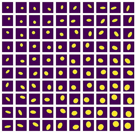
Figure 1: Elliptical disks used for the first numerical experiment. The opposing images with respect to the diagonal form isometrical pairs resulting from rotations and shifts.

TABLE I: Quantitative comparison between the computed gLGW distances. The first row shows the employed reference spaces $\SS_{1},\dots,\SS_{9}$, which include uniform distributions on different shapes as well as non-uniform distributions on the square $\SS_{3}$ and the two circles $\SS_{8}$. The distribution is indicated by the color of the pixels. For each reference, the computation time to compute all pairwise distances, the Mean Relative Error (MRE), and the Pearson Correlation Coefficient (PCC) as well as the number of non-zero points in the reference are recorded.

reference	GW	$\SS_{1}$	$\SS_{2}$	$\SS_{3}$	$\SS_{4}$	$\SS_{5}$	$\SS_{6}$	$\SS_{7}$	$\SS_{8}$	$\SS_{9}$
time	159.38 min	2.78 min	15.92 min	11.77 min	0.13 min	1.54 min	5.45 min	7.68 min	8.28 min	2.06 min
MRE	—	0.336	0.325	0.312	0.158	0.038	0.030	0.017	0.016	0.019
PCC	—	0.891	0.876	0.887	0.986	0.999	0.999	0.999	0.999	0.999
points	—	441	676	625	52	289	545	882	882	317

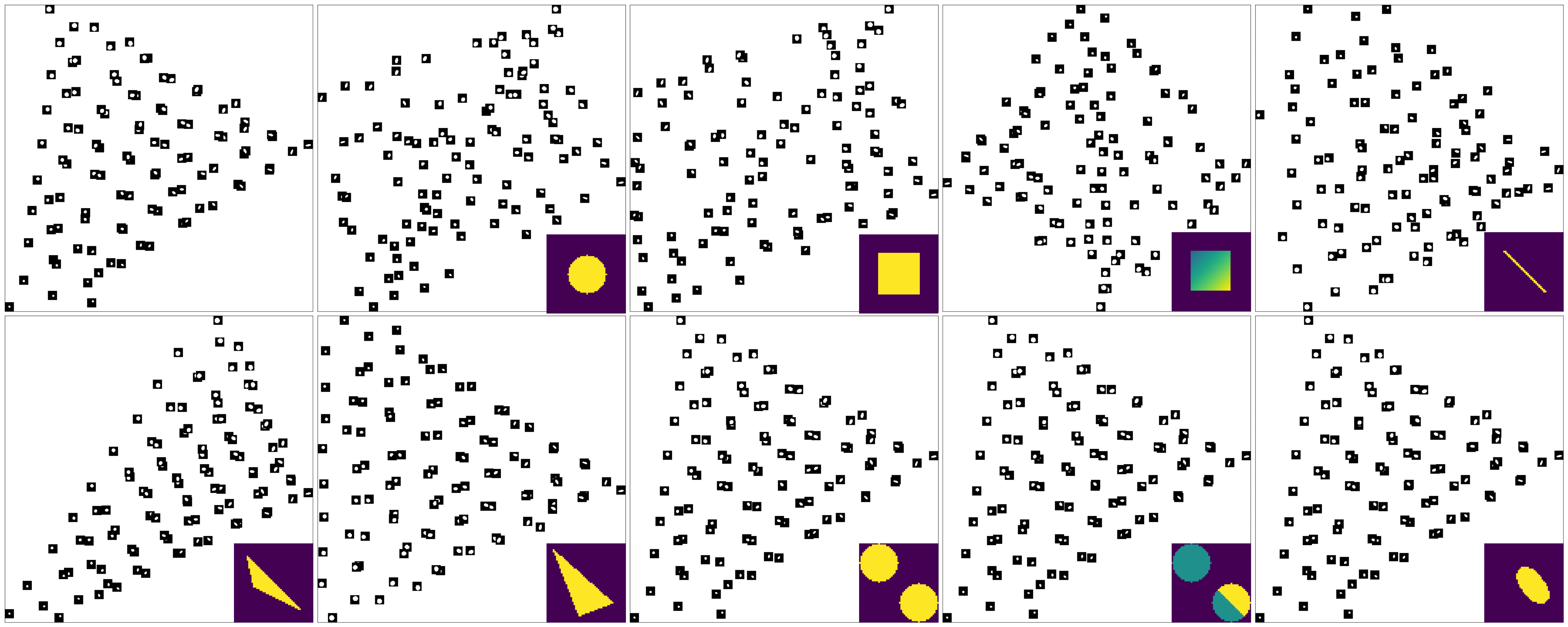
Figure 2: MDS embdding of the computed pairwise GW distances (top left) and the gLGW distances based on the references in Table I.

IV-A Gromov–Wasserstein of elliptical disks

For our first example, we apply $\operatorname{gLGW}$ to a toy problem, where we want to compute the GW distance between a series of elliptical disks, see Figure 1. Each image here consists of $50\times 50$ equispaced pixels in $[0,50]^{2}$. For the numerical simulations, we interpret these images as discrete mm-spaces $\mathbb{X}_{1},\dots,\mathbb{X}_{100}$. For this we set $\mathbb{X}_{k}\coloneqq([0,50]^{2},d_{\mathrm{E}},\mu_{k})$, where $d_{\mathrm{E}}$ is the Euclidean distance and $\mu_{k}$ corresponds the uniform distribution on the position of the white pixels. Notice that, except for the diagonal, all elliptical disks in Figure 1 occur in isometrical pairs (up to discretization errors). Since the GW distance is invariant under isometries, this should be reflected in the computed $\operatorname{GW}$ and $\operatorname{gLGW}$ distances.

For comparison, we first compute all pairwise GW distances, where we use the optimal Wasserstein coupling as starting value for the corresponding POT algorithm in the GW distance computation. We visualize them by embedding the images as points in the plane using MDS. The results is shown in Figure 2 (top left). Here the GW distance behaves as expected meaning that the isometrical pairs are found and located close to each other—the small visible distances between them result from the chosen discretizations. Up to this expected doubling, we essentially obtain a triangle, whose corners correspond to the smallest as well as the largest (isotopic) elliptical disk and the most anisotropic elliptical disk. The 4950 pairwise GW distances of this toy example have been computed in 159.38 minutes.

As mentioned in Remark III.3, the quality of the approximation of GW by LGW and thus gLGW strongly depends on the chosen reference space $\SS$. The choice of $\SS$ is especially crucial since the minimization over $\Pi_{\mathrm{o}}(\SS,\mathbb{X})$ and $\Pi_{\mathrm{o}}(\SS,\mathbb{Y})$ in (22) is numerical intractable, and fixed optimal plans $\pi_{\SS}^{\mathbb{X}}$ and $\pi_{\SS}^{\mathbb{Y}}$ are used instead. In the sense of Lemma III.2, natural choices for $\SS$ are circular or elliptical disks, but we also study uniform distributions on squares, triangles, lines as well as composed and non-uniform references. The employed references are shown in Table I.

To visually compare the approximation quality of $\operatorname{gLGW}_{\SS_{i}}$ for the considered references $\SS_{i}$, the computed distances are again embedded using MDS, see Figure 2. For more quantitative comparisons, we use the Mean Relative Error (MRE) and the Pearson Correlation Coefficient (PCC), which has been suggested in [34] to compare distances. The computed values are recorded in Table I. The impact of the different references is clearly visible raising again the question about a good reference.

The poorest performances correspond to the circular disk $\SS_{1}$ and the square $\SS_{2}$, which have a more regular shape than the others. Notice that, for any measure-preserving isometry $I:S_{i}\to S_{i}$ and any optimal plan $\pi_{\SS_{i}}^{\mathbb{X}_{k}}\in\Pi_{\mathrm{o}}(\SS_{i},\mathbb{X}_{k})$, we have

$$(I,\operatorname*{id})_{\#}\pi_{\SS_{i}}^{\mathbb{X}_{k}}\in\Pi_{\mathrm{o}}(\SS_{i},\mathbb{X}_{k});$$ (25)

so the larger the number of measure-preserving isometries of $\SS_{i}$, the larger the cardinality of $\Pi_{\mathrm{o}}(\SS_{i},\mathbb{X}_{k})$. Since the square $\SS_{2}$ is invariant under 3 rotations and 4 reflections and the circular disk $\SS_{1}$ nearly under arbitrary rotations and reflections, the minimization over all optimal plans in (22) cannot be neglected any more. This issue can also be observed numerically by examining the computed plans between the references $\SS_{1}$, $\SS_{2}$ and the given mm-spaces $\mathbb{X}_{k}$ in Figure 3. Considering the first two columns, we notice that the mass that is transported to the semi-minor axes of the first target is transported to the semi-major axes of the second target. Heuristically. $\operatorname{gLGW}_{\SS_{i}}$ is the evaluation of the GW objective in (10) with respect to the plan

$$\pi\coloneqq\Bigl{(}\mathcal{T}_{\pi_{\SS_{i}}^{\mathbb{X}_{k}}},\mathcal{T}_{\pi_{\SS_{i}}^{\mathbb{X}_{\ell}}}\Bigr{)}_{\#}\sigma_{k},$$

where $\mathcal{T}_{\bullet}$ is the generalized barycentric projection in (21). (Notice that $\pi$ may not satisfy the marginal constraints.) In this specific instance, the resulting plan $\pi$ essentially couples the semi-minor axis of the first target with the semi-major axis of the second target, which is clearly not optimal in the GW sense. The consequence of this matching issue is that $\operatorname{gLGW}_{\SS_{1}}$ and $\operatorname{gLGW}_{\SS_{2}}$ cannot recognize the isometric pairs, which is well reflected by the MDS embedding in Figure 2. Although the results of $\SS_{3}$ are slightly better, the non-uniform distribution on the square is not able to resolve this issue numerically. For the remaining references, this problem does not occur since there exist no isomorphic self-couplings or the self-couplings corresponds to the self-couplings of the target $\mathbb{X}_{k}$—rotation by 180° and reflections along the semi-major and semi-minor axes.

Figure 3: Examples of optimal GW plans between the reference mm-spaces (top) and two elliptical disks (middle, bottom) from Figure 1. The color indicates the mass transport from $\SS_{i}$ to $\mathbb{X}_{k}$ that is used for the barycentric projection.

The computation of the 4950 pairwise gLGW distances only requires 100 GW transport plans; therefore we obtain significant speed-ups in term of computation time. Considering the qualitative and quantitative results in Figure 2 and Table I, we notice that the specific computation time and the MRE strongly depend on the number support points in the reference space. The effect on the computation time is clear since optimal transport plans between spaces with less points can be calculated faster. The effect on the MRE is less obvious and seems to depend on the approximation of $\mathbb{X}_{k}$ by

$$\Bigl{(}\mathcal{T}_{\pi_{\SS_{i}}^{\mathbb{X}_{k}}}\Bigr{)}_{\#}\sigma_{k}.$$

Heuristically, the approximation becomes better and the MRE smaller, if the number of non-zero points in the reference is increased. Although the MRE with respect to the measure on the line $\SS_{4}$ is large, $\operatorname{gLGW}_{\SS_{4}}$ is well correlated to GW.

On the basis of the numerical experiments, a good reference measure is characterized by

• the number of isomorphic GW self-couplings (the less, the better) and

• the number of non-zero points (comparable to the number in the target spaces).

Finally, the elliptical disk reference $\SS_{9}$, which is close in the GW distance to all given $\mathbb{X}_{k}$, and which should be a good reference in the sense of Remark III.3, behaves as expected and give excellent results.

IV-B Gromov–Wasserstein in 2D shape analysis

Next, we apply the GW distance and its linear form to distinguish different 2D shapes from each other. In this numerical experiment, we use the publicly available database [35] embracing over 1 200 shapes in 70 shape classes. For our example, we select 20 shapes of the classes bone, goblet, star, and horseshoe, respectively, so that we obtain $80$ shapes in total. The shapes are stored as black and white images of different sizes, where the white pixels corresponds to the objects. To speed-up the computations, each images is approximated by a point measure $\mu_{k}$ consisting of 50 points and uniform weights. For this preprocessing step, we use the dithering technique in [36], see also [37]. All measures are randomly rotated yielding 80 mm-spaces $\mathbb{X}_{k}=([-1,1]^{2},\|\cdot\|,\mu_{k})$. A preprocessed example of each class is shown in Figure 4.

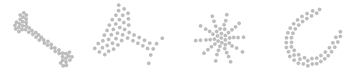
Figure 4: One example of each class (bone, goblet, star, horseshoe) of the employed 2D shape dataset.

The performance of the generalized linear GW distance again depends on the selection of an appropriate reference space $\SS$. As discussed in Remark III.3, a barycenter of $\mathbb{X}_{1},\dots,\mathbb{X}_{80}$ would be a natural choice. However, minimizing (24) with respect to $80$ inputs is numerically challenging. Considering the current state-of-the-art algorithm in [29], which is based on a blockwise coordinate descent, we have to compute an optimal GW plan for every input $\mathbb{X}_{k}$ per iteration; so the barycenter computation completely counteracts the computational speed-up by gLGW. To overcome this issue, we may either approximate the barycenter by performing only a few iterations or exploit that the mm-spaces within the different classes are already close to each other. Following the second approach, we choose a representative for each of the four classes to ensure that all main features are covered and compute a barycenter with 35 points and uniform weights. The employed barycenter is shown in Figure 5. Using the POT package, the computation takes 1.60 seconds. Since the reference $\SS$ has less points than the spaces $\mathbb{X}_{k}$, the barycentric projection (7) is indeed a mapping to weighted means.

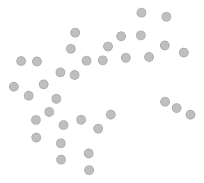
Figure 5: Embedding of the computed barycenter $\SS$ into $\mathbb{R}^{2}$ using MDS.

On the basis of the chosen reference $\SS$, we now compute the pairwise GW distances (11.34 seconds) and the pairwise gLGW distances (0.72 seconds). Even with barycenter computation, gLGW gives a significant speed-up against GW. The results are shown in Figure 6. Notice that the shapes in the horseshoe class significantly differ between each other explaining the greater distances than in other classes. In this example, the computed GW and gLGW distances are visually comparable. A more quantitative comparison is given below.

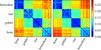
Figure 6: Pairwise GW distances (left) and generalized linear GW distances for a barycenter reference $\SS$. All images share the same color coding.

Considering the results, it seems reasonable to use a nearest neighbor classification to distinguish the different classes with respect to some representatives. Numerically, this concept may be verified by computing a confusion matrix consisting of the probabilities to classify an instance of a class as another class. For this, we rely on [19, § 8.2], where the confusion matrix is estimated by randomly choosing a representative for each class and then classifying all other shapes $\mathbb{X}_{k}$, $k=1,\dots,80$, with respect to the nearest representative. This classification task is then repeated 10 000 times. The confusion matrix of $\operatorname{GW}$ and $\operatorname{gLGW}$ are shown in Figure 7. Interestingly, gLGW performs slightly better than GW.

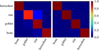
Figure 7: Confusion matrix for the GW distances (left) and the generalized linear GW distances with barycenter reference (right).

TABLE II: Quantitative comparisons of the 10-fold cross-validation. The recorded values correspond to the mean over all 10 training and classification tasks. The SVM has been trained based on gLGW, where barycenters of different sizes have been used.

points in barycenter	15	25	35	45	55
mean accuracy	0.9750	0.9625	0.9875	0.975	0.9875
mean MRE	0.2449	0.3040	0.1623	0.1826	0.1709
mean PCC	0.8042	0.7875	0.8936	0.8836	0.8904

The nearest neighbor classification already shows that the distinctiveness of gLGW is comparable to GW. To provide a more quantitative study, we combine gLGW with a support vector machine (SVM), see for instance [38] and references therein. Following the approach in [39], we employ the kernels $\exp(-\alpha\operatorname{GW})$ and $\exp(-\alpha\operatorname{gLGW}_{\SS})$ with $\alpha>0$ although these might not be positive definite. We obtain the best performance for $\alpha\coloneqq 10$. Moreover, we apply a 10-fold cross-validation. For this, we divide the given dataset $\mathbb{X}_{1},\dots,\mathbb{X}_{80}$ with respect to the classes into 10 disjoint subsets. In each iteration of the cross-validation, we train the SVM based on 9/10 of the data and use the remaining 1/10 data as test set. Further, the employed barycenter $\SS$ is computed anew from random representatives of the four classes with respect to the current training set. After each training, we compute the empirical success rate (accuracy) of the classification according to the current test set as well as the MRE and PCC between GW and gLGW. The means over all 10 cross-validation steps for different sizes of the barycenter are recorded in Table II. Note that the SVM with respect to the GW distance achieves a perfect accuracy score of one. Using gLGW, we encounter up to three misclassifications over all 10 cross-validation steps in total. Considering the mean classification accuracy, we may reduce the size of the barycenter to 15 points, which additionally speeds up the barycenter and gLGW computations. The MRE and PCC are improved for higher numbers. Both reach their optimum at around 35 points, which corresponds to the former given qualitative results. The appropriate number of points in the barycenter thus mainly depends on the application. If we are interested in classification, we may choose less points; if we are interested in pairwise GW approximations, we require more points.

IV-C Gromov–Wasserstein in 3D shape analysis

The GW distance traces back to the comparison and matching of 3D shapes, which we take up in our final numerical example. Analytically, a 3D shape is a two-dimensional submanifold of $\mathbb{R}^{3}$ that may have a boundary. 3D shapes can be interpreted as mm-spaces $\mathbb{X}=(X,d_{X},\mu)$, where $X$ is a surface of the shape, where $d_{X}$ corresponds to the length of the geodesics between two points, and where $\mu$ is some measure.

In practice, 3D shapes are usually triangulated and thus realized by a net of triangles. To handle them numerically, we approximate them by a discrete mm-space $\mathbb{X}=(X,d_{X},\mu)$. The vertices of the net become the discrete points in $X$. To approximate the geodesic distance on $X$, a weighted graph $G=(X,E)$ consisting of all vertices $X$ and all edges $E$ of the triangulation may be used, where the edges are weighted by the Euclidean distance between the corresponding vertices. The geodesic distance between two vertices may now be approximated by the length of the shortest path between these vertices. This distance can be computed by the Dijkstra algorithm from the NetworkX package [33]. The probability measure $\mu$ may be used to incorporate additional information of the shapes.

In this example, we consider 3D shapes of the publicly available database [40], which has already been used by Mémoli [19, § 8.2] in the context of GW distances. We use a similar setting to make the results comparable. As dataset for the experiment, we choose 3D shapes corresponding to the animals camel, cat, elephant, horse, and lion as well as to a human face and head. Each object is shown in 10 to 11 different poses totaling to 73 shapes. Figure 8 shows one example pose of each object. Every object is provided by a triangulation consisting of up to 43.000 vertices and up to 130.000 triangles.

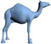
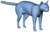
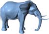
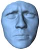
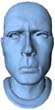
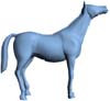
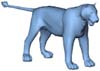
Figure 8: One example of each class (camel, cat, elephant, face, head, horse, lion) of the employed 3D shape dataset.

Since the discrete mm-spaces of the full triangulations consist of too many points for our purpose, the 3D shapes are preprocessed by a two-step approximation similar to [19].

1. Starting from a given triangulation with vertices $X$, we first reduce $X$ to a set $\widetilde{X}$ consisting of 4 000 vertices. The first vertex is hereby chosen randomly and is sequentially followed by the points with the largest Euclidean distance to the already chosen points. This selection rule is also known as the furthest point procedure.

2. The set $\widetilde{X}$ is reduced further and an appropriate measure $\mu$ is constructed. For this, we again apply the furthest point procedure to reduce $\widetilde{X}$ to a subset $\widehat{X}$ consisting of 50 points, but this time with respect to the discrete geodesic distance $d_{X}$ calculated using a weighted graph as explained above. Then we endow $\widehat{X}$ with a discrete probability measure, where the mass at $x\in\widehat{X}$ is proportional to the amount of closest neighbors within $\widetilde{X}$ with respect to the original geodesic distance $d_{X}$. In other words, we compute the Voronoi diagram of $\widetilde{X}$ to the points $\widehat{X}$ with respect to $d_{X}$ and count the members of each Voronoi cell. Repeating this procedure for every given 3D shape, we end up with 73 discrete mm-spaces $\mathbb{X}_{k}=(\widehat{X}_{k},d_{X_{k}},\mu_{k})$, $k=1,\dots,73$.

Since the distance $d_{X}$ of the constructed mm-spaces $\mathbb{X}_{k}$ are discrete geodesic distances, which are restricted to the points in $\widehat{X}_{k}$, the barycentric projection (21) has the form

$$\mathcal{T}_{\pi_{\SS}^{\mathbb{X}_{k}}}(s)\coloneqq\operatorname*{argmin}_{x_{0}\in\widehat{X}_{k}}\sum_{x\in\widehat{X}_{k}}\pi_{\SS}^{\mathbb{X}_{k}}({\{(s,x)\}})\,{d_{X_{k}}^{2}(x_{0},x)},$$

where $\pi_{\SS}^{\mathbb{X}_{k}}$ is the chosen optimal GW transport plan.

The pairwise GW distances (14.29 seconds) and the generalized linear GW distances (0.82 seconds) for the 3D shape dataset with respect to two different reference measures are shown in Figure 9. Similarly to the 2D shape example in Section IV-B, one of the considered references is a GW barycenter. To speed-up the computations, we again choose one representative of each class. To compute the barycenter with 50 points corresponding to a uniform distribution, the POT package needs around 4.67 seconds. Considering the middle image of Figure 9, we notice that gLGW is again comparable to GW, i.e. the different classes are clearly identifiable. Analogously to the previous numerical examples, and as indicated by Remark III.3, the barycenter gives excellent results. Since the computation of the barycenter is, however, numerically costly, we secondly use the given reduced 3D shape $\SS\coloneqq\mathbb{X}_{10}$ (camel) as reference. Here, the quality of the GW approximation illustrated in the right-hand side image of Figure 9 is more diverse. On the one side, the approximation of the GW distances inside the camel class is nearly perfect; on the other side, the approximation outside the camel class loses in quality. Especially, the head and face classes are affected.

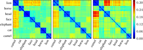
Figure 9: Pairwise GW distances (left), generalized linear GW distances for a barycenter reference $\SS$ (middle), and generalized linear GW distances with reference $\SS=\mathbb{X}_{10}$ (camel) (right). All images share the same color coding.

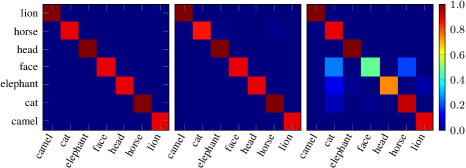
Figure 10: Confusion matrices for the GW distances (left), the generalized linear GW distance with barycenter reference (middle), and the generalized linear GW distance with reference $\SS=\mathbb{X}_{10}$ (right).

To evaluate the classification quality of the $\operatorname{GW}$ and $\operatorname{gLGW}$ distances, we compute the confusion matrix $C$ for both distances as in Section IV-B. The confusion matrix $C$ consists of the probabilities to classify a 3D shape within one class (camel, cat, elephant, face, head, horse, lion) to another class. Following again [19, § 8.2], for this purpose, we first randomly chose a representative for each class and then classify all 3D shapes $\mathbb{X}_{k}$, $k=1,\dots,73$, with respect to the nearest representative. This classification task is repeated 10 000 times. The result is shown in Figure 10. Considering the first two confusion matrices, we notice that the results for GW (left) and gLGW with barycenter reference (middle) nearly coincide. The classification based on gLGW with reference $\mathbb{X}_{10}$ (right) performs slightly worse. Camel $\mathbb{X}_{10}$ allow the classification of all four-legged animals. The serious misclassifications occur for the head and, especially, the face class, which is not astonishing since the geometry of $\mathbb{X}_{10}$ is quite differently from these two classes.

TABLE III: Mean MRE achieved during a 10-fold cross-validation. For each data splitting a new barycenter is computed. The experiment is repeated for different numbers of support points in the reduced graph and in the barycenter. The last row records the mean MRE for the camel reference $\mathbb{X}_{10}$.

	points in graph
points in barycenter	25	50	75	100
25	0.2339	0.1659	0.1687	0.1745
50	0.1975	0.1598	0.1486	0.1425
75	0.2408	0.1884	0.1798	0.1586
100	0.2417	0.2083	0.1799	0.1641
camel $\mathbb{X}_{10}$	0.2204	0.2124	0.2179	0.2618

TABLE IV: Mean PCC achieved during a 10-fold cross-validation. For each data splitting a new barycenter is computed. The experiment is repeated for different numbers of support points in the reduced graph and in the barycenter. The last row records the mean PCC for the camel reference $\mathbb{X}_{10}$.

	points in graph
points in barycenter	25	50	75	100
25	0.7577	0.8225	0.8452	0.8282
50	0.8686	0.9251	0.9268	0.9318
75	0.8537	0.9055	0.9156	0.9302
100	0.8769	0.9080	0.9212	0.9370
camel $\mathbb{X}_{10}$	0.7300	0.8428	0.8511	0.8496

TABLE V: Mean accuracy achieved during a 10-fold cross-validation. For each data splitting a new barycenter is computed. The experiment is repeated for different numbers of support points in the reduced graph and in the barycenter. The last row records the mean accuracy for the camel reference $\mathbb{X}_{10}$.

	points in graph
points in barycenter	25	50	75	100
25	0.9482	1.0000	0.9875	0.9714
50	0.9875	0.9857	1.0000	0.9857
75	0.9607	1.0000	1.0000	0.9857
100	1.0000	1.0000	0.9857	0.9750
camel $\mathbb{X}_{10}$	0.8535	0.9250	0.8964	0.9107

Similarly to the previous experiment, we train a SVM with respect to $\exp(-\alpha\operatorname{GW})$ and $\exp(-\alpha\operatorname{gLGW}_{\SS})$ with $\alpha\coloneqq 10$. The parameter choice $\alpha=10$ has again performed best. During the applied 10-fold cross-validation, a new barycenter is computed for every data splitting from one random representative of each class in the training set. Moreover, we repeat the cross-validation for different sizes of the reduced graphs, i.e. numbers of support points in $\widehat{X}_{k}$, and different sizes of the barycenter. The resulting MRE and PCC are recorded in Table III and IV. The best performance is obtained for the constellations of 50 points in the barycenter and 50 or more points in the reduced graph. Comparing both tables, we notice that the gLGW procedure performs best if the number of support points in the barycenter is less or equal the number of support points in the target spaces. As comparison, the last row in each table records the performance of gLGW with $\SS=\mathbb{X}_{10}$, where the number of points in the reference and the reduced graph coincide, and where the datum $\mathbb{X}_{10}$ has been removed from the training and testing subsets. Moreover, the SVM based on GW archives perfect accuracy scores of one. The accuracy with respect to gLGW is recorded in Table V. Although there are some misclassifications with respect to the head and face classes, the accuracy score for the camel reference $\SS=\mathbb{X}_{10}$ is high. The numerical experiments show that the classification by the SVM with gLGW is powerful even for non-optimal references.

V Conclusions

We proposed a linear version of the GW distance that was inspired by a generalized version of the linear Wasserstein distance. As the latter one, the approach appears to be efficient in applications, where pairwise distances of a larger amount of measures are of interest. We gave three examples indicating that our linear version of the GW distance gives reasonable approximations and circumvents the heavy computation of all pairwise distances. In contrast to Wasserstein distances, the mathematics behind GW distances is not well-examined so far and there are plenty of open problems which could be tackled in the future. For example, in generalized version of LOT, it would also be possible to use the concept of weak optimal transport [41]. This approach was neither considered for gLOT nor for gLGW so far. Further, multimarginals may be addressed, see [42]. Finally, we are interested in further applications in the context of shape and graph analysis. More precisely, we would like to incorporate our generalized linear Gromov–Wasserstein distance into existing shape and graph classification approaches exploiting feature spaces, annotations, and deep learning.

Appendix A Proofs

A-A Proof of Proposition II.4

We have that $\tilde{\mu}\in\mathcal{P}_{2}(\mathbb{R}^{d})$ since by Jensen’s inequality

$$\int_{\mathbb{R}^{d}}\|x\|^{2}\,\mathrm{d}\tilde{\mu}(x)$$

$$=\int_{\mathbb{R}^{d}}\|\mathcal{T}_{\pi_{\sigma}^{\mu}}(s)\|^{2}\,\mathrm{d}\sigma(s)=\int_{\mathbb{R}^{d}}\biggl{\|}\int_{\mathbb{R}^{d}}x\,\mathrm{d}\mathcal{\pi}_{s}(x)\biggr{\|}^{2}\,\mathrm{d}\sigma(s)$$

$$\leq\int_{\mathbb{R}^{d}}\int_{\mathbb{R}^{d}}\|x\|^{2}\,\mathrm{d}\pi_{s}(x)\,\mathrm{d}\sigma(s)=\int_{\mathbb{R}^{d}\times\mathbb{R}^{d}}\|x\|^{2}\,\mathrm{d}\pi_{\sigma}^{\mu}(s,x)$$

$$=\int_{\mathbb{R}^{d}}\|x\|^{2}\,\mathrm{d}\mu(x)<\infty.$$

Let $\pi_{\sigma}^{\tilde{\mu}}$ be an optimal transport plan with respect to $W(\sigma,\tilde{\mu})$. By the dual formulation of the optimal transport problem, see [27, Thm 4.2] and [25, Thm 5.10], we know that

$$\int_{\mathbb{R}^{d}\times\mathbb{R}^{d}}\frac{1}{2}\|s-x\|^{2}\,\mathrm{d}\pi_{\sigma}^{\tilde{\mu}}(s,x)$$ (26)

$$=\sup_{\phi\in L^{1}_{\sigma}(\mathbb{R}^{d})}\biggl{\{}\int_{\mathbb{R}^{d}}\phi(s)\,\mathrm{d}\sigma(s)+\int_{\mathbb{R}^{d}}\phi^{c}(x)\,\mathrm{d}\tilde{\mu}(x)\biggr{\}},$$ (27)

where $\phi^{c}$ denotes the $c$-concave function given by

$$\phi^{c}(x)=\inf_{y\in X}\{\tfrac{1}{2}\|x-y\|^{2}-\phi(y)\}.$$

To yield a contradiction, assume that $\mathcal{T}_{\pi_{\sigma}^{\mu}}$ is not an optimal transport map. Then

$$\tilde{\pi}\coloneqq(\operatorname*{id},\mathcal{T}_{\pi_{\sigma}^{\mu}})_{\#}\sigma$$

is not an optimal transport plan with respect to $W(\sigma,\tilde{\mu})$ and

$$\int_{\mathbb{R}^{d}}\frac{1}{2}\|s-\mathcal{T}_{\pi_{\sigma}^{\mu}}(s)\|^{2}\,\mathrm{d}\sigma(s)$$ (28)

$$=\int_{\mathbb{R}^{d}\times\mathbb{R}^{d}}\frac{1}{2}\|s-x\|^{2}\,\mathrm{d}\tilde{\pi}(s,x)$$

$$>\sup_{\phi\in L^{1}_{\sigma}(\mathbb{R}^{d})}\biggl{\{}\int_{\mathbb{R}^{d}}\phi(s)\,\mathrm{d}\sigma(s)+\int_{\mathbb{R}^{d}}\phi^{c}(x)\,\mathrm{d}\tilde{\mu}(x)\biggr{\}}.$$ (29)

Now we obtain for the optimal transport plan $\pi_{\sigma}^{\mu}$ of $W(\sigma,\mu)$ that

$$\int_{\mathbb{R}^{d}\times\mathbb{R}^{d}}\|s-x\|^{2}\,\mathrm{d}\pi_{\sigma}^{\mu}(s,x)$$

$$=\int_{\mathbb{R}^{d}}\|s\|^{2}\,\mathrm{d}\sigma(s)-2\int_{\mathbb{R}}^{d}\int_{\mathbb{R}}^{d}\langle s,x\rangle\,\mathrm{d}\pi_{s}(x)\,\mathrm{d}\sigma(s)$$

$$\qquad+\int_{\mathbb{R}^{d}}\|x\|^{2}\,\mathrm{d}\mu(x)$$

$$=\int_{\mathbb{R}^{d}}\|s\|^{2}\,\mathrm{d}\sigma(s)-2\int_{\mathbb{R}}^{d}\langle s,\mathcal{T}_{\pi_{\sigma}^{\mu}}(s)\rangle\,\mathrm{d}\sigma(s)$$

$$\qquad+\int_{\mathbb{R}^{d}}\|x\|^{2}\,\mathrm{d}\mu(x)$$

$$=\int_{\mathbb{R}^{d}}\|s-\mathcal{T}_{\pi_{\sigma}^{\mu}}(s)\|^{2}\,\mathrm{d}\sigma(s)+\int_{\mathbb{R}^{d}}\|x\|^{2}\,\mathrm{d}\mu(x)$$

$$\qquad-\int_{\mathbb{R}^{d}}\|x\|^{2}\,\mathrm{d}\tilde{\mu}(x)$$

and by (29) further

$$\int_{\mathbb{R}^{d}\times\mathbb{R}^{d}}\frac{1}{2}\|s-x\|^{2}\,\mathrm{d}\pi_{\sigma}^{\mu}(s,x)$$ (30)

$$>\int_{\mathbb{R}^{d}}\frac{1}{2}\|x\|^{2}\,\mathrm{d}\mu(x)-\int_{\mathbb{R}^{d}}\frac{1}{2}\|x\|^{2}\,\mathrm{d}\tilde{\mu}(x)$$ (31)

$$\qquad+\sup_{\phi\in L^{1}_{\sigma}(\mathbb{R}^{d})}\biggl{\{}\int_{\mathbb{R}^{d}}\phi(s)\,\mathrm{d}\sigma(s)+\int_{\mathbb{R}^{d}}\phi^{c}(x)\,\mathrm{d}\tilde{\mu}(x)\biggr{\}}$$ (32)

$$=\sup_{\phi\in L^{1}_{\sigma}(\mathbb{R}^{d})}\biggl{\{}\int_{\mathbb{R}^{d}}\frac{1}{2}\|x\|^{2}\,\mathrm{d}\mu(x)-\int_{\mathbb{R}^{d}}\frac{1}{2}\|x\|^{2}\,\mathrm{d}\tilde{\mu}(x)$$ (33)

$$\qquad+\int_{\mathbb{R}^{d}}\phi(s)\,\mathrm{d}\sigma(s)+\int_{\mathbb{R}^{d}}\phi^{c}(x)\,\mathrm{d}\tilde{\mu}(x)\biggr{\}}$$ (34)

$$=\sup_{\phi\in L^{1}_{\sigma}(\mathbb{R}^{d})}\biggl{\{}\int_{\mathbb{R}^{d}}\frac{1}{2}\|x\|^{2}\,\mathrm{d}\mu(x)+\int_{\mathbb{R}^{d}}\phi(s)\,\mathrm{d}\sigma(s)$$ (35)

$$\qquad+\int_{\mathbb{R}^{d}}\phi^{c}(x)-\frac{1}{2}\|x\|^{2}\,\mathrm{d}\tilde{\mu}(x)\biggr{\}},$$ (36)

where $L^{1}_{\sigma}(\mathbb{R}^{d})$ is the space of functions which absolute values are integrable with respect to $\sigma$. Since $\phi^{c}$ is $c$-concave, we know that $h\coloneqq\phi^{c}-\tfrac{1}{2}\|\cdot\|^{2}$ is concave, see [27, Lect 4.4]. Thus, Jensen’s inequality implies

$$\int_{\mathbb{R}^{d}}\phi^{c}(x)-\frac{1}{2}\|x\|^{2}\,\mathrm{d}\tilde{\mu}(x)$$ (37)

$$=\int_{\mathbb{R}^{d}}\phi^{c}(\mathcal{T}_{\pi_{\sigma}^{\mu}}(s))-\frac{1}{2}\|\mathcal{T}_{\pi_{\sigma}^{\mu}}(s)\|^{2}\,\mathrm{d}\sigma(s)$$ (38)

$$=\int_{\mathbb{R}^{d}}h\left(\mathcal{T}_{\pi_{\sigma}^{\mu}}(s)\right)\,\mathrm{d}\sigma(x)$$ (39)

$$=\int_{\mathbb{R}^{d}}h\left(\int_{\mathbb{R}^{d}}x\,\mathrm{d}\pi_{s}(x)\right)\,\mathrm{d}\sigma(s)$$ (40)

$$\geq\int_{\mathbb{R}^{d}}\int_{\mathbb{R}^{d}}h(x)\,\mathrm{d}\pi_{s}(x)\,\mathrm{d}\sigma(s)$$ (41)

$$=\int_{\mathbb{R}^{d}}\int_{\mathbb{R}^{d}}\phi^{c}(x)-\frac{1}{2}\|x\|^{2}\,\mathrm{d}\pi_{s}(x)\,\mathrm{d}\sigma(s)$$ (42)

$$=\int_{\mathbb{R}^{d}}\phi^{c}(x)\,\mathrm{d}\mu(x)-\int_{\mathbb{R}^{d}}\frac{1}{2}\|x\|^{2}\,\mathrm{d}\mu(x).$$ (43)

Inserting (43) into (36), we obtain

$$\int_{\mathbb{R}^{d}\times\mathbb{R}^{d}}\frac{1}{2}\|s-x\|^{2}\,\mathrm{d}\pi_{\sigma}^{\mu}(s,x)$$

$$>\sup_{\phi\in L^{1}_{\sigma}(\mathbb{R}^{d})}\biggl{\{}\int_{\mathbb{R}^{d}}\phi(s)\,\mathrm{d}\sigma(s)+\int_{\mathbb{R}^{d}}\phi^{c}(x)\,\mathrm{d}\mu(x)\biggr{\}},$$

which contradicts the optimality of $\pi_{\sigma}^{\mu}$. $\Box$

A-B Proof of Proposition III.1

To compute the distance (16), recall that the geodesics related to $\pi_{\SS}^{\mathbb{X}}\in\Pi_{\mathrm{o}}(\SS,\mathbb{X})$ and $\pi_{\SS}^{\mathbb{Y}}\in\Pi_{\mathrm{o}}(\SS,\mathbb{Y})$ are mapped to the tangents

$$g\coloneqq F_{\SS}(\pi_{\SS}^{\mathbb{X}}) =d_{X}-d_{S} (\text{acting on}\;\mathbb{T}_{g}\coloneqq(S\times X,d_{S},\pi_{\SS}^{\mathbb{X}})),$$

$$h\coloneqq F_{\SS}(\pi_{\SS}^{\mathbb{Y}}) =d_{Y}-d_{S} (\text{acting on}\;\mathbb{T}_{h}\coloneqq(S\times Y,d_{S},\pi_{\SS}^{\mathbb{Y}})),$$

where $\SS\sim\mathbb{T}_{g}\sim\mathbb{T}_{h}$. We next characterize the plans $\pi\in\Pi_{\mathrm{o}}(\mathbb{T}_{g},\mathbb{T}_{h})$ occurring in the definition of $\operatorname{GW}_{\SS}$ in (14). Since $\mathbb{T}_{g}$ and $\mathbb{T}_{h}$ are equivalent, each plan $\pi\in\Pi_{\mathrm{o}}(\mathbb{T}_{g},\mathbb{T}_{h})$ satisfies

$$0 =\operatorname{GW}(\mathbb{T}_{g},\mathbb{T}_{h})$$

$$=\int_{(S\times X\times S\times Y)^{2}}|d_{S}(s_{1},s_{2})-d_{S}(s_{1}^{\prime},s_{2}^{\prime})|^{2}$$

$$\hskip 80.0pt\times\,\mathrm{d}\pi(s_{1},x,s_{2},y)\,\mathrm{d}\pi(s_{1}^{\prime},x^{\prime},s_{2}^{\prime},y^{\prime}),$$

$$=\int_{(S\times S)^{2}}|d_{S}(s_{1},s_{2})-d_{S}(s_{1}^{\prime},s_{2}^{\prime})|^{2}\,\mathrm{d}\gamma(s_{1},s_{2})\,\mathrm{d}\gamma(s_{1}^{\prime},s_{2}^{\prime}),$$

where $\gamma\coloneqq P^{13}_{\#}\pi$. Thus, $\gamma$ is an optimal self-coupling of $\SS$ in the GW sense. As stated in [19, Lem 10.4], each self-coupling has the form $\gamma=(\operatorname*{id},\psi)_{\#}\sigma$ for some measure-preserving isometry $\psi:S\to S$. This, however, implies that the mapping $P^{124}(s_{1},x,s_{2},y)=(s_{1},x,y)$ is $\pi$-almost everywhere invertible by $(P^{124})^{-1}(s,x,y)=(s,x,\psi(s),y)$. More precisely, $(P^{124})^{-1}\circ P^{124}$ is the identity on $\textnormal{supp}(\pi)$. Therefore, we have

$$\pi=(P^{124})^{-1}_{\#}\tilde{\pi}\quad\text{with}\quad\tilde{\pi}=P^{124}_{\#}\pi.$$

Considering the marginals of $\tilde{\pi}$, we conclude that every 4-plan $\pi\in\Pi_{\mathrm{o}}(\mathbb{T}_{g},\mathbb{T}_{h})$ can be uniquely identified by the 3-plan $\tilde{\pi}\in{\Gamma}_{\SS}(\pi_{\SS}^{\mathbb{X}},\pi_{\SS}^{\mathbb{Y}})$, and vice versa. This identification finally allows us to rewrite the metric (14) on the tangent space using the substitution $\pi=(P^{124})^{-1}_{\#}\tilde{\pi}$ to obtain

$$\operatorname{GW}_{\SS}(\pi_{\SS}^{\mathbb{X}},\pi_{\SS}^{\mathbb{Y}})$$

$$=\inf_{\pi\in\Pi_{\mathrm{o}}(\mathbb{T}_{g},\mathbb{T}_{h})}\int_{(S\times X\times S\times Y)^{2}}\bigl{\lvert}d_{X}(x,x^{\prime})-d_{S}(s_{1},s_{1}^{\prime})$$

$$\hskip 100.0pt-d_{Y}(y,y^{\prime})+d_{S}(s_{2},s_{2}^{\prime})\bigr{\rvert}^{2}$$

$$\hskip 100.0pt\times\,\mathrm{d}\pi(s_{1},x,s_{2},y)\,\mathrm{d}\pi(s_{1}^{\prime},x^{\prime},s_{2}^{\prime},y^{\prime}),$$

$$=\inf_{\tilde{\pi}\in{\Gamma}_{\SS}(\pi_{\SS}^{\mathbb{X}},\pi_{\SS}^{\mathbb{Y}})}\int_{(S\times X\times Y)^{2}}\bigl{\lvert}d_{X}(x,x^{\prime})-d_{Y}(y,y^{\prime})$$

$$\hskip 115.0pt+d_{S}(\psi(s),\psi(s^{\prime}))-d_{S}(s,s^{\prime})\bigr{\rvert}^{2}$$

$$\hskip 115.0pt\times\,\mathrm{d}\tilde{\pi}(s,x,y)\,\mathrm{d}\tilde{\pi}(s^{\prime},x^{\prime},y^{\prime}),$$

$$=\inf_{\tilde{\pi}\in{\Gamma}_{\SS}(\pi_{\SS}^{\mathbb{X}},\pi_{\SS}^{\mathbb{Y}})}\int_{(S\times X\times Y)^{2}}\lvert d_{X}(x,x^{\prime})-d_{Y}(y,y^{\prime})\rvert^{2}$$

$$\hskip 132.0pt\times\,\mathrm{d}\tilde{\pi}(s,x,y)\,\mathrm{d}\tilde{\pi}(s^{\prime},x^{\prime},y^{\prime}),$$

which establishes the assertion. $\Box$

A-C Proof of Lemma III.2

For every $\pi_{\SS}^{\mathbb{X}}\in\Pi_{\mathrm{o}}(\SS,\mathbb{X})$ and $\pi_{\SS}^{\mathbb{Y}}\in\Pi_{\mathrm{o}}(\SS,\mathbb{Y})$ in (18), a three-plan $\pi\in{\Gamma}_{\SS}(\pi_{\SS}^{\mathbb{X}},\pi_{\SS}^{\mathbb{Y}})$ in (III.1) satisfies $P^{23}_{\#}\pi\in\Pi(\mu,\nu)$. Hence $\operatorname{GW}(\mathbb{X},\mathbb{Y})\leq\operatorname{LGW}_{\SS}(\mathbb{X},\mathbb{Y})$. For the upper bound, we consider fixed $\pi_{\SS}^{\mathbb{X}}\in\Pi_{\mathrm{o}}(\SS,\mathbb{X})$ and $\pi_{\SS}^{\mathbb{Y}}\in\Pi_{\mathrm{o}}(\SS,\mathbb{Y})$ in the definition of $\operatorname{LGW}_{\SS}$ in (18). Exploiting the definition of $\operatorname{GW}_{\SS}$ in (16) and the metric (14), we have

$$\operatorname{GW}_{\SS}(\pi_{\SS}^{\mathbb{X}},\pi_{\SS}^{\mathbb{Y}}) =\operatorname{GW}_{\SS}(d_{X}-d_{S},d_{Y}-d_{S})$$

$$\leq\operatorname{GW}_{\SS}(d_{X}-d_{S},0)+\operatorname{GW}_{\SS}(d_{Y}-d_{S},0),$$

where $0$ denotes the zero function on $S\times X$. Using the representatives $\mathbb{T}_{d_{X}-d_{S}}\coloneqq(S\times X,d_{X}-d_{S},\pi_{\SS}^{\mathbb{X}})$ and $\mathbb{T}_{0}\coloneqq(S\times X,0,\pi_{\SS}^{\mathbb{X}})$, we further obtain

$$\operatorname{GW}_{\SS}(d_{X}-d_{S},0)$$

$$=\inf\bigl{\{}\|d_{X}-d_{S}\|_{L^{2}((S\times X)^{4},\pi\otimes\pi)}:\pi\in\Pi_{\mathrm{o}}(\mathbb{T}_{d_{X}-d_{S}},\mathbb{T}_{0})\bigr{\}}$$

$$=\inf_{\pi\in\Pi_{\mathrm{o}}(\mathbb{T}_{d_{S}-d_{X}},\mathbb{T}_{0})}\int_{(S\times X\times S\times X)^{2}}|d_{X}(x_{1},x_{1}^{\prime})-d_{S}(s_{1},s_{1}^{\prime})|$$

$$\hskip 87.0pt\times\,\mathrm{d}\pi(s_{1},x_{1},s_{2},x_{2})\,\mathrm{d}\pi(s_{1}^{\prime},x_{1}^{\prime},s_{2}^{\prime},x_{2}^{\prime})$$

$$=\int_{(S\times X)^{2}}|d_{X}(s_{1},x_{1})-d_{S}(s_{1}^{\prime},x_{1}^{\prime})|\,\mathrm{d}\pi_{\SS}^{\mathbb{X}}(x_{1},s_{1})\,\mathrm{d}\pi_{\SS}^{\mathbb{X}}(x_{1}^{\prime},s_{1}^{\prime})$$

$$=\operatorname{GW}(\SS,\mathbb{X})$$

since $P^{12}_{\#}\pi=\pi_{\SS}^{\mathbb{X}}$ for all $\pi\in\Pi_{\mathrm{o}}(\mathbb{T}_{d_{X}-d_{S}},\mathbb{T}_{0})$. A similar computation shows $\operatorname{GW}_{\SS}(d_{Y}-d_{S},0)=\operatorname{GW}(\SS,\mathbb{Y})$. Thus $\operatorname{LGW}_{\SS}(\mathbb{X},\mathbb{Y})\leq\operatorname{GW}(\SS,\mathbb{X})+\operatorname{GW}(\SS,\mathbb{Y})$ as desired. $\Box$

Florian Beier studied mathematics at the Technical University Berlin. After recieving his MSc in 2021, he started his PhD under the supervision of Gabriele Steidl. His main research interest is Optimal Transport.

Robert Beinert received his PhD in Mathematics from the University of Göttingen (Germany). After a Postdoc at the University of Graz (Austria), he is currently a research fellow at the TU Berlin (Germany). His research interests include Inverse Problems, Optimization, Harmonic Analysis, and Convex Analysis with applications in Signal and Image Processing like Phase Retrieval.

Gabriele Steidl received her PhD and habilitation in mathematics from the University of Rostock. After positions as associated professor for Mathematics at the TU Darmstadt and full professor at the University of Mannheim and TU Kaiserslautern, she is currently professor at the TU Berlin. She was a Postdoc, resp. visiting Professor at the Univ. of Debrecen, Zürich, ENS Cachan/Paris Univ. Paris Est, Sorbonne/IHP Paris and worked as consultant of the Fraunhofer ITWM Kaiserslautern. Gabriele Steidl is Editor-in-Chief of the SIAM Journal of Imaging Sciences and SIAM Fellow. Her research interests include Harmonic Analysis, Optimization, Inverse Problem and Machine Learning with applications in Image Processing.

References

- [1] W. Wang, D. Slepčev, S. Basu, J. A. Ozolek, and G. K. Rohde, “A linear optimal transportation framework for quantifying and visualizing variations in sets of images,” Int. J. Comput. Vis., vol. 101, no. 2, pp. 254–269, 2013.
- [2] L. Ambrosio, N. Gigli, and G. Savaré, Gradient Flows in Metric Spaces and in the Space of Probability Measures. Birkhäuser, Basel, 2005.
- [3] W. Wang, J. A. Ozolek, D. Slepčev, A. B. Lee, C. Chen, and G. K. Rohde, “An optimal transportation approach for nuclear structure-based pathology,” IEEE Trans. Med. Imaging, vol. 30, no. 3, pp. 621–631, 2011.
- [4] A. H. M. Rubaiyat, K. M. Hallam, J. M. Nichols, M. N. Hutchinson, S. Li, and G. K. Rohde, “Parametric signal estimation using the cumulative distribution transform,” IEEE Trans. Signal Process., vol. 68, no. 68, pp. 3312–3324, 2020.
- [5] S. Kolouri, A. Tosun, J. Ozolek, and G. Rohde, “A continuous linear optimal transport approach for pattern analysis in image datasets,” Pattern Recognition, vol. 51, pp. 453–462, 2016.
- [6] S. Park, S. Kolouri, S. Kundu, and G. Rohde, “The cumulative distribution transform and linear pattern classification,” Appl. Comput. Harmon. Anal., 2017.
- [7] T. H. Emerson and J. M. Nichols, “Fitting local, low-dimensional parameterizations of optical turbulencemodeled from optimal transport velocity vectors,” Pattern Recognition Lett., vol. 133, pp. 123–128, 2020.
- [8] S. Basu, S. Kolouri, and G. Rohde, “Detecting and visualizing cell phenotype differences from microscopy images using transport-based morphometry,” Proc. Natl. Acad. Sci. USA, vol. 111, no. 9, pp. 3448–3453, 2014.
- [9] J. Ozolek, A. Tosun, W. Wang, C. Chen, S. Kolouri, S. Basu, H. Huang, and G. Rohde, “Accurate diagnosis of thyroid follicular lesions from nuclear morphology using supervised learning,” Med. Image. Anal., vol. 18, no. 5, pp. 772–780, 2014.
- [10] A. B. Tosun, O. Yergiyev, S. Kolouri, J. F. Silverman, and G. K. Rohde, “Detection of malignant mesothelioma using nuclear structure of mesothelial cells in effusion cytology specimens,” Cytometry Part A, vol. 87, no. 4, pp. 326–333, 2015.
- [11] M. Eckermann, B. Schmitzer, F. van der Meer, J. Franz, O. Hansen, C. Stadelmann, and T. Salditt, “Three-dimensional virtual histology of the human hippocampus based on phase-contrast computed tomography,” PNAS, vol. 118, no. 48, p. e2113835118, 2021.
- [12] S. Guan, B. Liao, Y. Du, and X. Yin, “Vehicle type recognition based on Radon-CDT hybrid transfer learning,” IEEE 10th International Conference on Software Engineering and Service Science (ICSESS), pp. 1–4, 2019.
- [13] S. R. Park, L. Cattell, J. M. Nichols, A. Watnik, T. Doster, and G. K. Rohde, “De-multiplexing vortex modes in optical communications using transport-based pattern recognition,” Opt. Express, vol. 26, no. 4, pp. 4004–4022, 2018.
- [14] S. Kolouri, S. Park, and G. Rohde, “The Radon cumulative distribution transform and its application to image classification,” IEEE Trans. Image Process., vol. 25, no. 2, pp. 920–934, 2016.
- [15] P. C. Álvarez-Esteban, E. del Barrioa, J. A. Cuesta-Albertos, and C. Matrán, “A fixed-point approach to barycenters in Wasserstein space,” J. Appl. Math. Anal. Appl., vol. 441, pp. 744–762, 2016.
- [16] A. Aldroubi, S. Li, and G. K. Rohde, “Partitioning signal classes using transport transformations for data analysis and machine learning,” arXiv:2008.03452v2, 2021.
- [17] C. Moosmüller and A. Cloninger, “Linear optimal transport embedding: Provable Wasserstein classification for certain rigid transformations and perturbations,” arXiv:2008.09165, 2021.
- [18] T. Cai, J. Cheng, B. Schmitzer, and M. Thorpe, “The linearized Hellinger-Kantorovich distance,” arXiv:2102.08807, 2021.
- [19] F. Mémoli, “Gromov–Wasserstein distances and the metric approach to object matching,” Found. Comput. Math., vol. 11, no. 4, pp. 417–487, 2011.
- [20] K.-T. Sturm, “The space of spaces: curvature bounds and gradient flows on the space of metric measure spaces,” arXiv:1208.0434, 2020.
- [21] F. Mémoli and T. Needham, “Distance distributions and inverse problems for metric measure spaces,” arXiv:1810.09646, 2021.
- [22] T. Vayer, R. Flamary, N. Courty, R. Tavenard, and L. Chapel, “Sliced Gromov-Wasserstein,” in Advances in Neural Information Processing Systems, H. Wallach, H. Larochelle, A. Beygelzimer, F. Alché-Buc, E. Fox, and R. Garnett, Eds., vol. 32. Curran Associates, Inc., 2019. [Online]. Available: https://proceedings.neurips.cc/paper/2019/file/a9cc6694dc40736d7a2ec018ea566113-Paper.pdf
- [23] R. Beinert, C. Heiss, and G. Steidl, “On assignment problems related to Gromov–Wasserstein distances on the real line,” arXiv:2205.09006, 2022.
- [24] A. Salmona, J. Delon, and A. Desolneux, “Gromov-Wasserstein distances between Gaussian distributions,” arXiv:2104.07970, 2021.
- [25] C. Villani, Optimal Transport: Old and New. Springer, 2008, vol. 338.
- [26] Y. Brenier, “Décomposition polaire et réarrangement monotone des champs de vecteurs,” Comptes rendus de l’Académie des Sciences, Paris, Série I, vol. 305, pp. 805–808, 1987.
- [27] L. Ambrosio, E. Brué, and D. Semola, Lectures on Optimal Transport, ser. Unitext. Cham: Springer, 2021, no. 130.
- [28] T. Vayer, “A contribution to optimal transport on incomplete spaces,” PhD Thesis, Université Bretagne, 2020.
- [29] G. Peyré, M. Cuturi, and J. Solomon, “Gromov-Wasserstein averaging of kernel and distance matrices,” in International Conference on Machine Learning, 2016, pp. 2664–2672.
- [30] ——, “Gromov-Wasserstein learning for graph matching and node embedding,” in International Conference on Machine Learning, 2019, pp. 6932–6941.
- [31] R. Flamary, N. Courty, A. Gramfort, M. Z. Alaya, A. Boisbunon, S. Chambon, L. Chapel, A. Corenflos, K. Fatras, N. Fournier, L. Gautheron, N. T. Gayraud, H. Janati, A. Rakotomamonjy, I. Redko, A. Rolet, A. Schutz, V. Seguy, D. J. Sutherland, R. Tavenard, A. Tong, and T. Vayer, “POT: Python optimal transport,” J. Mach. Learn. Res., vol. 22, no. 78, pp. 1–8, 2021. [Online]. Available: http://jmlr.org/papers/v22/20-451.html
- [32] F. Pedregosa, G. Varoquaux, A. Gramfort, V. Michel, B. Thirion, O. Grisel, M. Blondel, P. Prettenhofer, R. Weiss, V. Dubourg, J. Vanderplas, A. Passos, D. Cournapeau, M. Brucher, M. Perrot, and E. Duchesnay, “Scikit-learn: Machine learning in Python,” J. Mach. Learn. Res., vol. 12, pp. 2825–2830, 2011.
- [33] A. A. Hagberg, D. A. Schult, and P. J. Swart, “Exploring network structure, dynamics, and function using NetworkX,” in Proceedings of the 7th Python in Science Conference, G. Varoquaux, T. Vaught, and J. Millman, Eds., 2008, pp. 11–15.
- [34] C. Vincent-Cuaz, T. Vayer, R. Flamary, M. Corneli, and N. Courty, “Online graph dictionary learning,” in Proceedings of the 38th International Conference on Machine Learning, ser. Proceedings of Machine Learning Research, M. Meila and T. Zhang, Eds., vol. 139. PMLR, 18–24 Jul 2021, pp. 10 564–10 574.
- [35] A. Carlier, K. Leonard, S. Hahmann, G. Morin, and M. Collins, “The 2D shape structure dataset,” https://2dshapesstructure.github.io.
- [36] T. Teuber, G. Steidl, P. Gwosdek, C. Schmaltz, and J. Weickert, “Dithering by differences of convex functions,” SIAM J. Imaging Sci., vol. 4, no. 1, pp. 79–108, 2011.
- [37] M. Ehler, M. Gräf, S. Neumayer, and G. Steidl, “Curve based approximation of measures on manifolds by discrepancy minimization,” Foundations in Computational Mathematics, vol. 21, no. 6, pp. 1595–1642, 2021.
- [38] G. Steidl, “Supervised learning by support vector machines,” in Handbook of Mathematical Methods in Imaging, O. Scherzer, Ed. Springer, 2011, vol. 2, pp. 959–1014.
- [39] V. Titouan, N. Courty, R. Tavenard, C. Laetitia, and R. Flamary, “Optimal transport for structured data with application on graphs,” in Proceedings of the 36th International Conference on Machine Learning, ser. Proceedings of Machine Learning Research, K. Chaudhuri and R. Salakhutdinov, Eds., vol. 97. PMLR, 09–15 Jun 2019, pp. 6275–6284.
- [40] R. W. Sumner and J. Popovic, “Mesh data from deformation transfer for triangle meshes,” http://people.csail.mit.edu/sumner/research/deftransfer/data.html.
- [41] N. Gozlan, C. Roberto, P.-M. Samson, and P. Tetali, “Kantorovich duality for general transport costs and applications,” J. Funct. Anal., vol. 273, no. 11, pp. 3327–3405, 2017.
- [42] F. Beier, J. von Lindheim, S. Neumayer, and G. Steidl, “Unbalanced multi-marginal optimal transport,” arXiv:2103.10854, 2021.