——————————————————————————————————————————–

Abstract

Quintessential inflation provides a unified description of inflation and dark energy in terms of a single scalar degree of freedom, the cosmon. We present here a comprehensive overview of this appealing paradigm, highlighting its key ingredients and keeping a reasonable and homogeneous level of details. After summarizing the cosmological evolution in a simple canonical case, we discuss how quintessential inflation can be embedded in a more general scalar-tensor formulation and its relation to variable gravity scenarios. Particular emphasis is placed on the role played by symmetries. In particular, we discuss the evolution of the cosmon field in terms of ultraviolet and infrared fixed points potentially appearing in quantum gravity formulations and leading to the emergence of scale invariance in the early and late Universe. The second part of the review is devoted to the exploration of the phenomenological consequences of the paradigm. First, we discuss how direct couplings of the cosmon field to matter may affect neutrinos masses and primordial structure formation. Second, we describe how Ricci-mediated couplings to spectator fields can trigger the spontaneous symmetry breaking of internal symmetries such as, but not limited to, global U(1) or Z₂ symmetries, and affect a large variety of physical processes in the early Universe.

——————————————————————————————————————————–

bettoni@usal.es
javier.rubio@tecnico.ulisboa.pt

1 Introduction

“Once upon a time the Universe sped up, out of emptiness. Then, there was something all over the place. Lucky we were that it dawdled to hasten again, so we can be here to observe”.

The current best-fitting picture of the statistical properties of the Universe, from horizon scales ($15000$ Mpc) to typical galactic separations ($1$ Mpc), is the so-called $\Lambda$ Cold Dark Matter scenario ($\Lambda$CDM). This $6$-parameter model assumes the Universe to be composed of photons, neutrinos, ordinary matter and a non-relativistic or cold dark matter (CDM) component with gravitational interactions only. On top of that, it presumes the existence of two accelerated expansion eras taking place in the very early and the very late Universe: Inflation and Dark Energy.

1. Inflation: This epoch provides a natural solution to the shortcomings of the hot Big Bang (hBB) model, being able to generate, without finetunings, a flat, homogeneous and isotropic Universe while removing unwanted relics such as monopoles or other topological defects. More importantly, it provides a causal mechanism for the generation of the primordial density perturbations seeding structure formation. These fluctuations are unavoidably created out of the quantum vacuum and stretched out to superhorizon scales, where they become classical. In the simplest realizations, they are also adiabatic, Gaussian and display a nearly scale-invariant spectrum at all observable scales. On top of that, they remain frozen outside the horizon until they reenter it again long after the end of inflation. When doing so, they generate the coherent set of oscillations we observe in the Cosmic Microwave Background (CMB) and seed the large-scale distribution of matter and galaxies in the Universe. Interestingly enough, the results of three decades of observations are remarkably consistent with the simplest incarnation of the inflationary paradigm: a canonical scalar field slowly rolling in a featureless potential and eventually approaching a global minimum, where oscillations are effectively damped by the quanta production of the fields coupled to it.

   Beyond temperature and density fluctuations, inflation predicts a so-far unobserved background of tensor perturbations displaying also a quasi scale-invariant spectrum. The main signature of this stochastic gravitational wave background is a curl-like pattern in the CMB polarization. These $B$-modes are the target of several ongoing and forthcoming initiatives, ranging from ground-based experiments to stratospheric balloons and space missions [1]. Its detection would constitute the first test of the quantum nature of spacetime, while providing an indirect window to fundamental physics all the way up to the unification scale.

2. Dark energy: The discovery in the late 90’s of the current accelerated expansion of the Universe revolutionized modern cosmology [2, 3]. Since then, this result has been indirectly confirmed, among others, by CMB observations [4, 5] and large scale structure surveys [6, 7, 8]. In the context of General Relativity, the simplest mathematical explanation is a non-vanishing cosmological constant $\Lambda$ leading to a time-independent energy density of order $\rho_{\Lambda}\simeq(1\,{\rm meV})^{4}$. The inclusion of this everlasting component in a Universe where all other matter species redshift with expansion raises immediately two naturalness issues: i) why is the cosmological constant so small as compared to all particle physics scales? and ii) why did it start dominating precisely now? The lack of satisfactory answers to these questions has motivated a plethora of alternative explanations to the present accelerated expansion of the Universe, usually coined under the generic name of dark energy models. Many of these proposals involve a time-dependent (non-homogeneous) scalar field with an evolving equation of state different from that of baryons, neutrinos, dark matter, or radiation. This fifth or quintessential entity is generically designed to mimic, with sufficient accuracy, a de Sitter-like behaviour at the present cosmological epoch, in full analogy with the inflationary stage but at an energy scale many orders of magnitude lower. Interestingly enough, some quintessence scenarios involve appealing scaling solutions in which the dark energy density remains comparable to the dominant radiation and matter components for an extended period of time, eventually jumping out of this behaviour to drive the late-time acceleration. Provided that the event triggering this transition does not involve any additional tuning of times or scales, this alleviates the aforementioned “why now” problem.

Since inflation and quintessence typically require a beyond the Standard Model field to drive an almost de Sitter stage, it seems natural to seek for the unification of these two stages into a common framework, potentially based on an underlying symmetry principle. This is the main idea behind the so-called Quintessential inflation paradigm, where the inflaton and dark energy fields are identified as a single scalar component customarily dubbed cosmon [9]. This approach reduces the required number of degrees of freedom by one, with the further advantage of eliminating the problem of setting the initial conditions for the quintessence field, which are now determined by the standard inflationary attractor. When written in terms of a canonical scalar field, these scenarios involve a potential of runaway-type with two flat or slow-roll regions connected by a steep transition spanning more than hundred orders of magnitude. This large hierarchy of scales can be imposed by hand or follow naturally from some underlying principle, as happen for instance in quantum chromodynamics, where the existence of an ultraviolet (UV) fixed point makes the infrared (IR) confinement scale exponentially smaller than the UV cutoff of the theory. At the phenomenological level, the steep transition leads generically to an intermediate cosmological epoch in which the energy density of the Universe is dominated by the kinetic energy density of the cosmon field. During this period, the global equation of state of the Universe approaches unity and the total energy density decreases as the sixth power of the scale factor. This peculiar scaling might allow to discriminate quintessential inflation scenarios from standard oscillatory models. In fact, as we will discuss in detail in this review, there are several interesting phenomenological consequences associated to it. First, the fast dilution of the cosmon energy density implies that any other form of matter will eventually dominate the background evolution. This amplification effect has advantages and drawbacks. On the one hand, it allows to recover the standard hBB picture even if the cosmon field is only mildly depleted after inflation. On the other hand, it induces a substantial growth of any stochastic background of primordial gravitational waves at the corresponding scales, leading to potential violations of Big Bang Nucleosynthesis (BBN) constraints in scenarios involving very extended periods of kination.

Aim and spirit of this review: To make quantitative predictions within the quintessential inflation paradigm one can follow two major strategies: perform case-by-case studies involving specific choices of the cosmon potential or follow a first-principles observational-oriented approach. The first point of view has been widely explored in the literature [10, 11], from the early works of Refs. [12, 13, 14, 15, 16, 17, 18] to the most recent developments [19, 20, 21, 22, 23, 24, 25, 26, 27]. In this review, we will follow the second approach, trying to connect the behavior of the cosmon field to a minimum of quantities and principles. In particular, we aim to provide an overview of quintessential inflation for a wide audience, including both cosmologists and particle physicists. To cope with this goal, we have focused on the generic ingredients of the paradigm, keeping a reasonable and homogeneous level of details throughout the whole manuscript and intentionally avoided the exhaustive description of the myriad of models in the literature. Overall, this approach brings clarity at the expense of disguising the technical complexity of the issues we discuss, for which we refer the reader to Refs. [10, 11]. For the sake of concreteness, we also exclude from this review a number of theoretical topics, such as warm quintessential inflation [28], curvaton-inspired scenarios [29], higher-dimensional settings [30] and non-Riemannian approaches related to scale symmetry [31, 32].

This article is organized as follows. In Section 2, we overview the cosmological history of a canonically normalized cosmon field minimally coupled to gravity. After discussing the generalities of the inflationary stage in Section 2.1, we concentrate in Section 2.2 on the unusual kinetic dominated era, presenting the constraints on its duration imposed by BBN. Special attention is then given to the unconventional heating stage, which we describe in detail in Section 2.3, leaving for Section 2.4 the discussion of the standard hBB evolution and the onset of scalar domination at late times. The embedding of quintessential inflation in a more general variable gravity framework is presented in Section 3, where we summarize the alternative representations and equivalence classes in the literature. Section 4 discusses the potential association of quintessential inflation with the emergence of scale symmetry in the vicinity UV and IR fixed points, presenting the conditions for the absence of fifth-forces and the temporal non-variation of the Standard Model coupling constants. The last part of the review, Section 5, presents an extensive discussion of the expected phenomenology in the presence of interactions with a potential beyond the Standard Model sector. In particular, Section 5.1 describes the coupled quintessence paradigm and its applications in the context of growing neutrino quintessence and primordial structure formation, while Section 5.2 discusses the impact of non-minimal gravitational interactions and their effects on (re)heating, gravitational waves’ production and baryogenesis. Finally, in Section 6, we comment on the challenges and open avenues in this field of research.

Notation and conventions. We will work in natural units ($c=1$ and $\hbar=1$) and use a mostly plus signature for the metric (-,+,+,+).

2 Cosmological evolution

In its simplest form, quintessential inflation can be formulated in terms of a canonically-normalized scalar field minimally coupled to gravity. The corresponding action takes the form

$$S=\int d^{4}x\sqrt{-g}\left[\frac{M_{P}^{2}}{2}R-\frac{1}{2}(\partial\phi)^{2}-V(\phi)\right]+S_{\rm I}(g_{\mu\nu},\phi,\chi,A_{\mu},\psi)\,,$$ (1)

with $M_{P}=(8\pi G)^{-1/2}=2.44\times 10^{18}$ GeV the reduced Planck mass, $R$ the Ricci scalar and $(\partial\phi)^{2}$ a short hand notation for the kinetic term $g^{\mu\nu}\partial_{\mu}\phi\,\partial_{\nu}\phi$, with $g_{\mu\nu}$ the metric and $g={\rm det}\,(g_{\mu\nu})$ the metric determinant. The cosmon potential $V(\phi)$ is assumed to be of a runaway form and, as in any other dark energy-related models, it cannot innately explain why the observed cosmological constant is so negligibly small, making necessary the implementation of a symmetry principle or cancellation mechanism in order to explain its value. For the purposes of this review, we will simply assume that the cosmon potential vanishes asymptotically at large, positive field values, $V(\phi\rightarrow\infty)\rightarrow 0$, albeit presenting in Section 4 several arguments supporting this assumption. Finally, the action $S_{\rm I}$ encodes the interactions of the cosmon field with scalar ($\chi$), fermion ($\psi$) and vector ($A_{\mu}$) degrees of freedom in the Standard Model sector and beyond.

On a flat Friedman-Lemaître-Robertson-Walker (FLRW) Universe with diagonal metric $g_{\mu\nu}={\rm diag}(-1,a^{2}(t)\delta_{ij})$ and scale factor $a(t)$, the Friedman and Klein-Gordon equations following from the variation of the action (1) with respect to $g_{\mu\nu}$ and $\phi$ can be written as

$$H^{2}=\frac{1}{3M_{P}^{2}}\sum_{i}\rho_{i}\,,\hskip 17.07164pt\dot{H}=-\frac{1}{2M_{P}^{2}}\sum_{i}(\rho_{i}+p_{i})\,,\hskip 17.07164pt\ddot{\phi}+3H\dot{\phi}-a^{-2}\nabla^{2}\phi+V_{,\phi}=Q(\phi,\chi,A_{\mu},\psi)\,,$$ (2)

with the sum running over the cosmon field and all matter species in $S_{\rm I}$ and the $Q$ term accounting for the potential interactions among these components. Here $H\equiv\dot{a}/a$ is the Hubble expansion rate, the dots denote derivatives with respect to the coordinate time $t$, $\rho_{i}$ and $p_{i}$ stand for the energy densities and pressures of each component in $S$ and the subscript $\phi$ indicates a derivative with respect to the cosmon field. Assuming the contribution of all matter fields in $S_{\rm I}$ to be or become subdominant at very early and very late times, the dynamics of the system of equations in (2) becomes controlled by the energy density and pressure of the cosmon field at those epochs,

$$\rho_{\phi}=\frac{1}{2}\dot{\phi}^{2}+\frac{1}{2a^{2}}|\nabla\phi|^{2}+V\,,\hskip 28.45274pt\textrm{and}\hskip 28.45274ptp_{\phi}=\frac{1}{2}\dot{\phi}^{2}-\frac{1}{6a^{2}}|\nabla\phi|^{2}-V\,,$$ (3)

or equivalently by its energy density and the equation-of-state parameter

$$w_{\phi}\equiv\frac{p_{\phi}}{\rho_{\phi}}\,.$$ (4)

For a homogeneous scalar field, the latest quantity interpolates between a de Sitter value $w_{\phi}\simeq-1$ for potential domination, $V\gg\dot{\phi}^{2}$, and a stiff value $w_{\phi}\simeq+1$ for kinetic domination, $\dot{\phi}^{2}\gg V$. Thus, as illustrated in Fig. 1, the presence in the cosmon potential of two flat or slow-roll regions connected by a steep transition is a priori sufficient to generate two periods of exponential expansion at very different energy scales separated by a stage of kinetic domination. Of course, the wealth of available observational data ranging from CMB observations [4, 33] to BBN constraints [34] places several requirements in this model building process [35, 36, 22, 37]. For instance, a phenomenologically successful scenario should be able to generate the correct amplitude and tilt for the primordial power spectrum of density fluctuations, as well as to incorporate a stage of relativistic particle production giving rise to the onset of the hBB era. On top of that, this ambitious program requires the cosmon field to remain quiet and energetically subdominant for an extended period of time after particle creation, such that the standard radiation and matter dominated epochs have the sufficient duration. Eventually, the cosmon field must also exit its quiescence and start behaving as a quintessence component able to support the present accelerated expansion of the Universe, as depicted in Figs. 2 and 3. In what follows, we will provide a quick overview of the full cosmological evolution in this type of scenarios, going through the various stages with a minimum amount of details and referring to the extensive literature for more comprehensive analyses.

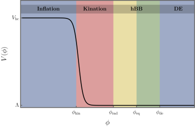
Figure 1: Schematic illustration of the quintessential inflation potential in canonically-normalized scenarios. The presence of two flat or slow-roll regions connected by a steep transition is a priori sufficient to generate two periods of exponential expansion separated by a stage of kinetic domination. Provided a sufficiently efficient creation of particles at the end of inflation, this setting allows also for the standard hot big bang evolution (radiation and matter domination).

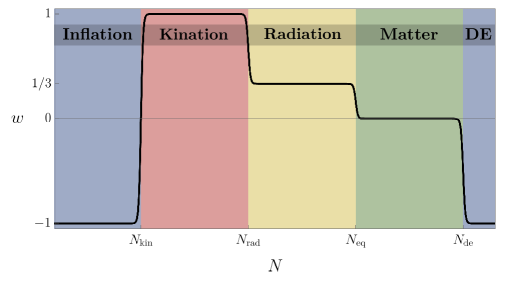
Figure 2: Cosmological evolution of the background equation of state in quintessential inflation scenarios. The lack of a potential minimum translates generically into the appearance of a kinetic dominated era immediately after the end of inflation ($w\simeq-1$), during which the global equation of state parameter is stiff ($w\simeq 1$). This unusual expansion history extends till the onset of radiation ($w=1/3$) and matter domination ($w=0$), where the cosmon field remains energetically subdominant. Eventually, it starts dominating again, giving rise to the current accelerated expansion of the Universe ($w\rightarrow-1$).

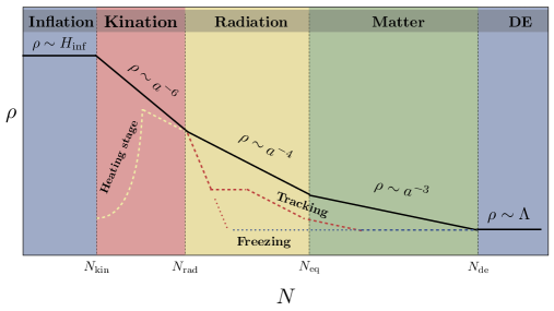
Figure 3: Schematic description of the cosmological evolution of the energy densities in quintessential inflation scenarios. The black, solid line corresponds to the dominant component density. The dashed lines correspond to subdominant radiation (yellow) and cosmon field (purple).

2.1 Inflation

The inflationary stage is assumed to start in a region of the Universe in which the cosmon evolution is sufficiently slow and the energy density stored in the potential term dominates the total energy budget, $V\gg 1/2\,\dot{\phi}^{2},\,1/2|\nabla\phi|^{2}$. As any other single-field scenario, these models benefits from a late-time attractor solution that makes the dynamics in phase space almost insensitive to the specific initial conditions [38]. In order to sustain inflation for an extended period of time, it is also necessary that the acceleration experienced by the cosmon is sufficiently small as compared with its velocity per Hubble time, $|\ddot{\phi}|\ll H|\dot{\phi}|$. Under these conditions, the first Friedman and Klein-Gordon equations in (2) become respectively

$$3M_{P}^{2}H^{2}\simeq V\,,\hskip 56.9055pt-V_{,\phi}\simeq 3H\dot{\phi}\,.$$ (5)

This slow-roll regime can be supported by a variety of potential shapes around the region of interest, including power-law forms [13, 14, 39], exponential profiles [22] and plateau-like behaviours [40, 41]. The main requirement is that the so-called slow-roll parameters

$$\epsilon\equiv\frac{M_{P}^{2}}{2}\left(\frac{V_{,\phi}}{V}\right)^{2}\,,\hskip 56.9055pt\eta\equiv M^{2}_{P}\frac{V_{,\phi\phi}}{V}\,,$$ (6)

encoding the local slope and curvature of the potential remain small for an extended period of time. More precisely, the condition $\epsilon\ll 1$ is required for the accelerated expansion to take place in the first place, while the requirement $|\eta|\ll 1$ ensures that it lasts long enough to solve the flatness and horizon problems. In the limit $\epsilon\approx 0$, the rate of expansion is approximately constant and the scale factor grows exponentially with time, $a\propto e^{Ht}$, leading to an almost de Sitter expansion. During the inflationary stage, scalar (s) and tensor (t) perturbations are created out of quantum vacuum fluctuations and spatially stretched to superhorizon scales [42, 43, 44, 45, 46], where they become classical and inherit almost scale-invariant spectra [42, 43, 44, 45, 46, 47, 48, 49, 50, 51]. At the leading order in the slow-roll parameters, these spectra take the parametric form

$${\cal P}_{s}={\cal A}_{s}\left(\frac{k}{k_{\rm hc}}\right)^{n_{s}-1}\,,\hskip 28.45274pt{\cal P}_{t}={\cal A}_{t}\left(\frac{k}{k_{\rm hc}}\right)^{n_{t}}\,,$$ (7)

with the corresponding amplitudes and tilts,

$$\mathcal{A}_{\,s} = \left.\frac{1}{2M_{P}^{2}\,\epsilon}\left(\frac{H}{2\pi}\right)^{2}\right|_{\rm hc}\,,\hskip 56.9055ptn_{s}=1-6\epsilon_{\rm hc}+2\eta_{\rm hc}\,,$$ (8)

$$\mathcal{A}_{\,t} = \left.\frac{8}{M_{P}^{2}}\left(\frac{H}{2\pi}\right)^{2}\right|_{\rm hc}\,,\hskip 71.13188ptn_{t}=-2\epsilon_{\rm hc}\,,$$ (9)

depending only on the potential term and its derivatives through the relation $H^{2}\simeq V/(3M_{P}^{2})$, and the subscript hc indicating the evaluation of the corresponding quantities at the horizon exit of a given reference scale $k^{-1}_{\rm hc}=(a_{\rm hc}H_{\rm hc})^{-1}$. Note that both ${\cal P}_{s}$ and ${\cal P}_{t}$ are time-independent as long as the associated fluctuations are outside the horizon, meaning that their amplitudes at horizon re-entry, and therefore the initial conditions for the subsequent causal evolution, are the same as those at the first horizon crossing. The ratio of the spectral amplitudes defines the so-called tensor-to-scalar ratio

$$r\equiv\left.\frac{\mathcal{A}_{\,t}}{{\mathcal{A}}_{s}}\right|_{\rm hc}=16\epsilon_{\rm hc}=-8n_{t}\,.$$ (10)

The last equality can be understood as a consistency relation for single field inflationary models. In particular, since we are working in Einstein gravity and the cosmon field satisfies the null energy condition, the Hubble rate decreases with time, leading to a red-tilted GW spectrum with negative tensor spectral tilt.

The horizon crossing of a given momentum scale can be related to the number of $e$-folds of inflation obtained by integrating the second equation in (5), namely

$$N\equiv\ln\frac{a_{\rm end}}{a}\simeq\frac{1}{M_{P}}\int_{\phi_{\rm end}}^{\phi}\frac{d\phi}{\sqrt{2\epsilon}}\,,$$ (11)

with $\phi_{\rm end}$ the value of the cosmon field following from the violation of the slow-roll conditions, ${\rm max}[\epsilon(\phi_{\rm end}),|\eta(\phi_{\rm end})|]=1$. In particular, for a scale $k^{-1}_{\rm hc}=(a_{\rm hc}H_{\rm hc})^{-1}$ reentering the horizon at the present cosmological epoch ($a_{\rm hc}H_{\rm hc}=a_{0}H_{0}$), we have

$$N_{\rm hc}=-\ln\left(\frac{H_{\rm end}}{H_{\rm hc}}\right)+\ln\left(\frac{a_{\rm end}H_{\rm end}}{a_{0}H_{0}}\right)\,.$$ (12)

The first term in this expression depends implicitly on the specific cosmon potential and therefore on the overall energy scale of inflation. The second one accounts for the complete post-inflationary evolution and, in particular, for any nonstandard expansion period, such as kinetic domination.

Recent observational constraints on the inflationary observables at a pivot scale $k_{\rm hc}=0.05\,{\rm Mpc}^{-1}$ are provided by the Planck and BICEP/Keck collaborations [4, 5],

$${\cal A}_{s} =(2.099\pm 0.014)\times 10^{-9}\hskip 28.45274pt \textrm{at 68\% CL}\,,$$ (13)

$$n_{s} =0.9649\pm 0.0042\hskip 48.36967pt \textrm{at 68\% CL}\,,$$ (14)

$$r <0.036\hskip 96.73936pt \textrm{at 95\% CL}\,.$$ (15)

Note that while the deviation of the scalar spectral tilt from unity is statistically significant, the precise value of the tensor-to-scalar ratio remains unknown, and with it the Hubble rate and the energy scale of inflation at the pivot scale. In particular, combining Eqs. (8) and (10) with the observed amplitude (13), we get

$$H_{\rm hc} = 7.9\times 10^{12}\,{\rm GeV}\left(\frac{r}{0.001}\right)^{1/2}\lesssim 4.7\times 10^{13}\leavevmode\nobreak\ \rm GeV\,,$$ (16)

$$V_{\rm hc}^{1/4} = 5.8\times 10^{15}\,{\rm GeV}\left(\frac{r}{0.001}\right)^{1/4}\lesssim 1.4\times 10^{16}\leavevmode\nobreak\ \rm GeV\,,$$ (17)

with the final bounds following directly from Eq. (15). The combination of this upper limit with the consistency relation (10) implies also that the tensor spectrum at CMB scales is almost exactly scale invariant, $-n_{t}\leq 0.0045\ll 1$, a condition that we will assume in what follows.

2.2 Kination

After the end of inflation, the cosmon field acquires a large kinetic energy density at the expenses of its potential counterpart, which rapidly becomes subdominant and irrelevant for the subsequent dynamics. This gives rise to a kinetic dominated era dubbed deflation [12] or kination [52] where the global equation of state of the Universe approaches the maximum value allowed by causality, $w=1$. During this unusual cosmological epoch, the Ricci scalar is negative [cf. Eq. (35)] and the first Friedmann and Klein-Gordon equations in (2) take the approximate form

$$3M_{P}^{2}H^{2}\simeq\frac{\dot{\phi}^{2}}{2}\,,\hskip 56.9055pt\ddot{\phi}+3H\dot{\phi}\simeq 0\,.$$ (18)

This system of equations admits a solution

$$\phi-\phi_{\rm kin}=\sqrt{6}\,M_{P}\,\Delta N_{\rm kin}\,,\hskip 56.9055ptH^{2}=H^{2}_{\rm kin}\left(\frac{a_{\rm kin}}{a}\right)^{6}\,,$$ (19)

with

$$\Delta N_{\rm kin}\equiv\log\left(\frac{a}{a_{\rm kin}}\right)$$ (20)

the number of $e$-folds of kination. The quantitative differences among the times, field values and energy scales in this expression (“kin”) and those at the end of inflation (“end”) depend on the specific model under consideration. However, for most practical purposes, they can be considered small and safely neglected. This allows us to identify the end of inflation with the onset of kination, i.e., $a_{\rm kin}=a_{\rm end}$, $\phi_{\rm kin}=\phi_{\rm end}$, $H_{\rm kin}=H_{\rm end}$.

The scaling of the Hubble rate in (19) affects a plethora of particle physics processes in the very early Universe, including, for instance, the generation of the matter-antimatter asymmetry [52, 53, 54] or the abundance of dark matter relics [55, 56, 57, 58, 59, 60, 61, 62, 63, 64]. Additionally, it enhances any stochastic background of gravitational waves of primordial origin, such as those generated by inflation [65, 66, 67, 39, 68, 69, 70, 71], preheating [72, 73, 74, 75, 76, 77], cosmic strings [78, 79, 80, 81, 82, 83] or phase transitions [84]; see Ref. [85] for a review. For the specific case of inflationary perturbations, a global stiff equation of state translates into an explicit breaking of scale invariance for modes reentering the horizon during kinetic domination. To see this, let us consider the present density parameter for GWs, customarily defined as the current GW energy-density $\rho_{\rm GW}(\tau_{0},k)$ per logarithmic interval of comoving momentum $k$ normalized to the critical density $\rho_{\rm crit}=3M_{P}^{2}H^{2}$, [65, 66, 39, 68], i.e.

$$\Omega_{\rm GW}^{(0)}(k)\equiv\dfrac{1}{\rho_{\text{crit}}}\dfrac{d\rho_{\rm GW}(\tau_{0},k)}{d\ln k}=\frac{1}{12}\left(\frac{k}{a_{0}H_{0}}\right)^{2}\Delta_{h}^{2}(\tau_{0},k)\,,$$ (21)

with

$$\Delta_{h}^{2}(\tau_{0},k)\equiv\frac{2k^{3}}{\pi^{2}}\left<|h_{k}(\tau_{0})|^{2}\right>$$ (22)

the ensemble-averaged spectrum of tensor perturbations $h_{k}$ at present time. These modes follow themselves from a Fourier decomposition

$$h_{ij}(\tau,\mathbf{x})=\sum_{\lambda}\int\frac{d^{3}\textbf{k}}{(2\pi)^{3}}e^{i\mathbf{k}.\mathbf{x}}\epsilon_{ij}^{\lambda}(\mathbf{k})h^{\lambda}_{\mathbf{k}}(\tau)\,,$$ (23)

with $h_{ij}$ a transverse-traceless metric perturbation ($\partial_{j}h_{ij}=h^{i}_{i}=0$) entering the linearized Einstein equations

$$h_{ij}^{\prime\prime}+2\frac{a^{\prime}}{a}h_{ij}^{\prime}-\nabla^{2}h_{ij}=0\,.$$ (24)

Here $\lambda=+,\times$ stand for the two physical graviton polarization states and $\epsilon_{ij}^{\lambda}(\mathbf{k})$ denotes a basis of polarization tensors, with $\epsilon_{ij}^{\lambda}(\mathbf{k})=\epsilon_{ji}^{\lambda}(\mathbf{k})$, $\epsilon_{ii}^{\lambda}(\mathbf{k})=0$, $k_{i}\epsilon_{ij}^{\lambda}(\mathbf{k})=0$, $\epsilon_{ij}^{\lambda}(\mathbf{k})=\epsilon_{ij}^{\lambda^{*}}(-\mathbf{k})$, $\epsilon_{ij}^{\lambda}(\mathbf{k})\epsilon_{ij}^{\sigma^{*}}(\mathbf{k})=2\delta^{\lambda\sigma}$. Assuming the tensor spectrum to be completely unpolarized and neglecting its small tilt $n_{t}\ll 1$ [5], the present GW energy density parameter in a Universe undergoing an epoch of kination between inflation and radiation domination takes the form [70]

$$\Omega_{\text{GW}}^{(0)}(k)\simeq\Omega_{\rm GW}^{(0)}{\Big{|}}_{\rm no-kin}\times\left\{\begin{array}[]{crl}1&\,,&\hskip 14.22636ptk\ll k_{\rm rad}\,,\vspace*{0.4cm}\\ \frac{4}{\pi}\,\left(\frac{k}{k_{\rm rad}}\right)&\,,&\hskip 14.22636ptk\gg k_{\rm rad}\,,\\ \end{array}\right.$$ (27)

with

$$\Omega_{\rm GW}^{(0)}{\Big{|}}_{\rm no-kin}\simeq\leavevmode\nobreak\ 5\cdot 10^{-22}\left(\frac{H_{\rm kin}}{10^{11}\,{\rm GeV}}\right)^{2}$$ (28)

the corresponding scale-invariant amplitude in the absence of kination and $k_{\rm rad}$ the momentum associated with the horizon scale at the onset of radiation domination.

The linear raising of (27) at high-momenta serves as an observational signature of quintessential inflation. At the same time, it limits the corresponding parameter space since the energy density of this relativistic component affects directly the expansion rate of the Universe and with it the abundance of light elements. In particular, BBN observations impose a limit on the integrated GW contribution to the total energy density [86, 68], namely

$$h^{2}\int_{k_{\text{BBN}}}^{k_{\rm kin}}\Omega^{(0)}_{\text{GW}}(k)d\ln k\leq 5.6\times 10^{-6}\,\Delta N_{\nu}\simeq 1.12\times 10^{-6}\,,$$ (29)

with $h=0.678$ the reduced Hubble constant, $k_{\rm kin}$ and $k_{\rm BBN}$ the momenta associated to the horizon scale at the onset of kination and BBN, and $\Delta N_{\nu}\lesssim 0.2$ an effective parameter encoding any extra amount of radiation beyond the Standard Model content [87, 88]. This bound applies to all sources of primordial gravitational waves and in particular to the specific inflationary background in Eq. (27). Taking into account the power law behaviour of this quantity, the integral in Eq. (29) can be approximated by its upper end, getting a simpler expression $h^{2}\Omega^{(0)}_{\text{GW}}(k\gg k_{\rm rad})\lesssim 1.12\times 10^{-6}$ that tends to exclude models with large inflationary scales and extended periods of kination.

2.3 Heating

The measured abundance of light elements indicates that our Universe was radiation dominated during BBN [34], thus setting a limit on the duration of the kinetic dominated era discussed in the previous section [89],

$$\Delta N_{\rm kin}\lesssim 27+\frac{1}{3}\ln\left(\frac{H_{\rm kin}}{10^{11}{\rm GeV}}\right)\,.$$ (30)

The end of this peculiar cosmological epoch will take place when the Universe becomes dominated by the energy density of a relativistic component, created potentially through the so-far irrelevant interaction terms in Eq. (1). Note, however, that the generation of a thermal bath in quintessential inflation cannot proceed as in the usual oscillatory models of inflation (for a review, see e.g. Refs. [90, 91]). First, the runaway character of the potential prevents the standard amplification of bosonic fields via parametric resonance [92]. Second, the cosmon field cannot directly interact with the Standard Model particles since that would induce the decay and destabilization of the scalar potential tail. Hence, a successful heating mechanism must proceed either through an indirect production of particles or involve a set of sufficiently efficient couplings to an auxiliary matter sector quickly shutting down the interaction and preventing the complete decay of the inflaton condensate. In either case, the cosmon energy density must dilute faster than the produced species or their decay products, in order to allow for the onset of a radiation dominated epoch.

The background energy density during kination is initially dominated by the cosmon field, which decays as $\rho_{\phi}\sim a^{-6}$. This rapid scaling translates into a relative amplification of any radiation component $\rho_{r}\sim a^{2}\rho_{\phi}$, making it eventually dominate the background evolution [93]. A convenient way of quantifying the duration of this stage while being agnostic on the particular model of heating is to introduce the concept of heating efficiency [39]. The simplest definition of this quantity involves the ratio between the energy density of the relativistic particles produced at the onset of kination and the energy density of the cosmon field at that time,

$$\Theta\equiv\frac{\rho_{r}^{\rm kin}}{\rho_{\phi}^{\rm kin}}=\left(\frac{a_{\rm kin}}{a_{\rm rad}}\right)^{2}\,.$$ (31)

Albeit this definition assumes instant heating, the concept of heating efficiency can be easily extended to non-instantaneous settings [39]. The important point to keep in mind, however, is that the detailed description of the process is not needed in practice. In other words, since the heating stage in quintessential inflation requires almost compulsory an external sector with new parameters, the introduction of a single one compressing that information is a convenient choice. For example, taking into account the value of the pivot scale $k_{\rm hc}=0.002\,{\rm Mpc}^{-1}=1.27\times 10^{-32}$ eV used in the derivation of the combined Planck/BICEP2 results [94], the number of relativistic degrees of freedom at matter-radiation equality $g_{\rm mat}=3.36$ and the present value of the radiation temperature $T_{0}\simeq 2.73\,{\rm K}\simeq 2.35\times 10^{-4}$ eV, we can rewrite the required number of e-folds of inflation in terms of the heating efficiency [39]

$$N\simeq 63.3+\frac{1}{4}\ln\left(\frac{r}{0.001}\right)-\frac{1}{4}\ln\left(\frac{\Theta}{10^{-8}}\right)\,.$$ (32)

Note that since comoving modes re-approach the Hubble scale faster during kination than during radiation or matter domination, the required number of $e$-folds needed to solve the flatness and horizon problems increases for smaller heating efficiencies. Assuming a fiducial value $H_{\rm kin}\sim 10^{11}$ GeV and taking into account that the heating efficiency per degree of freedom can vary between $\Theta\sim 10^{-19}$ and $\Theta\sim\mathcal{O}(1)$ depending on the specific heating mechanism [39] (see below), the minimal number of $e$-folds in quintessential inflation scenarios is typically in the range $60\lesssim N\lesssim 70$. Part of this window is, however, excluded by Big Bang Nucleosynthesis constraints. In particular, the integrated bound in Eq. (29) translates into a lower limit [39]

$$\Theta\gtrsim 10^{-16}\left(\frac{H_{\rm kin}}{10^{11}{\rm GeV}}\right)^{2}\,.$$ (33)

Several heating mechanisms based on the exponential amplification of quantum fluctuations via some kind of instability have been put forward over the years [93, 12, 95, 96, 97, 98, 99, 29, 100, 101, 102, 103, 24, 27]. On general grounds, they can be classified according to the presence or absence of direct couplings to auxiliary matter sectors and to whether they produce particles via adiabaticity violation or tachyonic instability. To illustrate this explicitly, let us consider the following action for an exemplary and energetically-subdominant scalar field $\chi$

$$S=\int d^{4}x\sqrt{-g}\left[-\frac{1}{2}(\partial\chi)^{2}-\frac{1}{2}(M^{2}(\phi)+\xi R)\chi^{2}\right]\,.$$ (34)

In this expression the inflaton field $\phi$ acts as a homogeneous background field, $M(\phi)$ is a field-dependent mass potentially including a bare mass contribution $m_{\chi}$, $\xi$ is a positive-definite non-minimal coupling and

$$R=3H^{2}(1-3w)$$ (35)

stands for the Ricci scalar in a FLRW background, written in terms the global equation of state $w$. Note that we have intentionally restricted ourselves to quadratic interactions in the scalar sector. This is indeed a good approximation for the first stages of kination, where the auxiliary field $\chi$ is close enough to the origin and particle production is most efficient. However, as we will see in Section 5.2, higher-order operators can play a crucial role at late times, especially in the presence of internal symmetries.

The evolution of the field $Y$ is more easily described in the conformal variables

$$\chi=\chi_{*}\frac{a_{\rm kin}}{a}Y\,,\quad\quad dz=a_{\rm kin}\chi_{*}d\tau\,,\quad\quad\vec{y}=a_{\rm kin}\chi_{*}\vec{x}\,,\qquad\vec{\kappa}=\frac{\vec{k}}{a_{\rm kin}\chi_{*}}\,,$$ (36)

with $d\tau=dt/a(t)$ the conformal time and $\chi_{*}$ a potentially convenient normalization. Introducing also the Fourier transform

$$Y(\vec{y},z)=\int\frac{d^{3}\kappa}{(2\pi)^{3/2}}Y_{\vec{\kappa}}(z)e^{i\vec{\kappa}\cdot\vec{y}}\,,$$ (37)

the equation of motion following from the variation of Eq. (34) with respect to $\chi$ can be written as

$$Y_{\vec{\kappa}}^{\prime\prime}+\omega^{2}_{\kappa}(z)Y_{\vec{\kappa}}=0\,,$$ (38)

with

$$\omega_{\kappa}^{2}(z)=\kappa^{2}+\frac{m_{\chi}^{2}+M^{2}_{\rm eff}(\phi)}{\chi_{*}^{2}}\left(\frac{a}{a_{\rm kin}}\right)^{2}-3\mathcal{H}^{2}(3w-1)\left(\xi-\frac{1}{6}\right)$$ (39)

an effective frequency term, $\kappa=|\vec{\kappa}|$ and $\mathcal{H}=a^{\prime}(z)/a(z)=a(z)H(z)$ the comoving Hubble rate.

The quantization of the scalar field $\chi$ proceeds according to the standard procedure [104, 105]. The function $Y_{\vec{\kappa}}$ is promoted to a quantum operator

$$\hat{Y}_{\vec{\kappa}}=\hat{a}_{\vec{\kappa}}f_{\kappa}(z)+\hat{a}^{\dagger}_{-\vec{\kappa}}f^{*}_{\kappa}(z)$$ (40)

satisfying the equal time commutation relations $[\hat{Y}_{\vec{\kappa}}(z),\hat{\Pi}_{\vec{\kappa}^{\prime}}(z)]=i\delta(\vec{\kappa}+\vec{\kappa}^{\prime})$, with $\hat{\Pi}_{\vec{\kappa}}=d\hat{Y}_{\vec{\kappa}}/dz$. Here, $a_{\vec{\kappa}}$ and $a^{\dagger}_{\vec{\kappa}^{\prime}}$ are annihilation and creation operators displaying equal-time commutation relations $[a_{\vec{\kappa}},a^{\dagger}_{\vec{\kappa}^{\prime}}]=\delta({\vec{\kappa}}-{\vec{\kappa}^{\prime}})\,,[a_{\vec{\kappa}},a_{\vec{\kappa}^{\prime}}]=[a^{\dagger}_{\vec{\kappa}},a^{\dagger}_{\vec{\kappa}^{\prime}}]=0$ and $f_{\kappa}$ is a set of isotropic mode functions satisfying

$$f_{\kappa}^{\prime\prime}+\omega^{2}_{\kappa}(z)f_{\kappa}=0\,,\hskip 56.9055pt2\,{\rm Im}(f^{\prime}_{\kappa}f^{*}_{\kappa})=1\,.$$ (41)

Note that the choice of the basis $\{f_{\kappa}(z),f^{*}_{\kappa}(z)\}$ is generically non unique, meaning that Eq. (40) should be understood as an implicit definition of the operators $\hat{a}$ and $\hat{a}^{\dagger}$. For constant positive square frequencies, a positive frequency mode $f_{\kappa}\propto e^{-i\omega t}$ defines a unique vacuum state $\hat{a}_{\vec{\kappa}}|0\rangle=0$. For non-constant non-positive square frequencies, the notion of vacuum become ambiguous. In particular, particle production can be achieved either because the adiabaticity condition $|\omega_{\kappa}^{\prime}|/\omega_{\kappa}^{2}<1$ is violated or because the frequency becomes tachyonic for a certain range of $\kappa$ modes, $\omega_{\kappa}^{2}<0$ (i.e. $\omega_{\kappa}$ is imaginary). Given the complications and extensive phenomenology of the latter scenario, we will postpone its analysis to Section 5.2, focusing in what follows on the simplest case $\omega^{2}_{\kappa}(z)>0$.

The amount of produced quanta for positive frequencies can be determined by comparing the instantaneous adiabatic vacua at two different times. Since the equation of motion (41) is second order, there must exist a linear Bogoliubov transformation between two mode expansions $f_{\kappa}$ and $h_{\kappa}$ evaluated at the same time, namely

$$f_{\kappa}(z)=\alpha_{\kappa}\,h_{\kappa}(z)+\beta_{\kappa}\,h^{*}_{\kappa}(z)\,,$$ (42)

with the coefficients $\alpha_{\beta}$ and $\beta_{\kappa}$ satisfying the normalization condition $|\alpha_{\kappa}|^{2}-|\beta_{\kappa}|^{2}=1$ following from the second expression in (41). As shown for instance in Ref. [105], the occupation number of a mode $\kappa$ is given by square of the second Bogoliubov coefficient $\beta_{\kappa}$,

$$n_{\kappa}(z)=\left|\beta_{\kappa}(z)\right|^{2}\,,$$ (43)

whose expression in terms of the mode expansion functions can be obtained by solving the associated equation with proper “in” and “out” vacuum conditions.

Given the occupation numbers $n_{\kappa}(z)$ one can compute the total number of $Y$ particles and the associated energy density

$$n(z)=\frac{1}{(2\pi)^{3}}\int d^{3}\vec{\kappa}\,\,n_{\kappa}(z)\,,\hskip 42.67912pt\rho(z)=\frac{1}{(2\pi)^{3}}\int d^{3}\vec{\kappa}\,\,\omega_{\kappa}(z)n_{\kappa}(z)\,.$$ (44)

The resulting spectrum is not expected to be thermal. In fact, heating mechanisms tend to amplify IR fluctuations below a given characteristic scale, leading to a spectral shape initially peaked at low momenta. The subsequent evolution of this overoccupied system proceeds typically through a rather slow process of driven and free turbulence [106, 107, 103], for which thermal techniques are not generically applicable. Still, it is sometimes convenient to define an instantaneous temperature or energy scale

$$T_{\rm r}(z)\equiv\left(\frac{30}{\pi^{2}g_{*}(z)}\,\rho_{\rm r}(z)\right)^{1/4}\,,$$ (45)

with $g_{*}(z)$ the effective number of relativistic degrees of freedom at a given time $z$. The (re)heating temperature $T_{r}(z_{\rm rad})$ signaling the onset of radiation domination is correspondingly defined by the condition $\rho_{\phi}(z_{\rm rad})=\rho_{r}(z_{rad})$. Assuming exact kination ($w=1$, $R=-6H^{2}$, $\rho_{\phi}\sim a^{-6}$), relativistic decay products ($\rho_{r}\sim a^{-4}$) and entropy conservation, this quantity can be related to the maximum instantaneous temperature or energy scale at the onset of kinetic domination, namely

$$T_{r}(z_{\rm rad})=\left(\frac{g_{*,s}(z_{\rm kin})}{g_{*,s}(z_{\rm rad})}\right)^{1/3}\Theta^{1/2}\,T_{r}(z_{\rm kin})\,,$$ (46)

with $g_{*,s}(z_{\rm kin})$ and $g_{*,s}(z_{\rm rad})$ the entropic degrees of freedom at the corresponding times. Accounting for all Standard Model degrees of freedom, $g_{*}(z_{\rm kin})=g_{*,s}(z_{\rm kin})=g_{*,s}(z_{\rm rad})=106.75$, we have

$$T_{r}(z_{\rm rad}) \simeq 2.7\times 10^{8}\leavevmode\nobreak\ {\rm GeV}\left(\frac{\Theta}{10^{-8}}\right)^{\frac{3}{4}}\left(\frac{H_{\rm kin}}{10^{11}\leavevmode\nobreak\ {\rm GeV}}\right)^{\frac{1}{2}}\,,$$ (47)

$$T_{r}(z_{\rm kin}) \simeq 2.7\times 10^{12}\leavevmode\nobreak\ {\rm GeV}\left(\frac{\Theta}{10^{-8}}\right)^{\frac{1}{4}}\left(\frac{H_{\rm kin}}{10^{11}\leavevmode\nobreak\ {\rm GeV}}\right)^{\frac{1}{2}}\lesssim 6\times 10^{15}\leavevmode\nobreak\ {\rm GeV}\,\Theta^{1/4}\,,$$ (48)

with the upper limit in the last expression following from (15) and the restriction (16).

Specific cases:

Having presented the generalities of preheating via violations of the adiabaticity condition $|\omega_{\kappa}^{\prime}|/\omega_{\kappa}^{2}<1$, let us discuss some specific mechanisms connected with the choices of functions and parameters in Eq. (39). As before, we assume exact kinetic domination ($w=1$, $R=-6H^{2}$).

• Gravitational heating [93, 12, 95]

  In this scenario, the production of particles is purely associated to the expansion of the Universe, being essentially triggered by any rapid change in the Ricci scalar $R$ [93, 108, 65]. This mechanism applies therefore to non-conformally coupled scalar fields only ($\xi\neq 1/6$), since the evolution equations of gauge bosons and chiral fermions in a conformally flat geometry are invariant under Weyl rescalings.

  For a light scalar field ($m_{\chi}\ll H_{\rm kin}$) in kinetic domination, the effective frequency in Eq. (39) takes the form

  $$\omega_{\kappa}^{2}=\begin{cases}\kappa^{2}+\mathcal{H}^{2}\,\quad&{\rm for}\quad\xi=0\,,\\ \kappa^{2}+(1-6\xi)\mathcal{H}^{2}\,\quad&{\rm for}\quad\xi<1/6\,,\end{cases}$$ (49)

  with the condition in the last expression ensuring that $\omega_{\kappa}^{2}$ is positive definite for all $\kappa$, such that the particle production is only due to adiabaticity violation and the Bogoliubov formalism presented above can be straightforwardly applied. The case with $\xi>1/6$ is analyzed in detail in Section 5.2.

  During a Hubble time in kinetic domination, the variation of the (relativistic) energy density per spectator field is of the order $\Delta\rho_{r}\sim\delta\times(\Delta H)^{4}\sim(\Delta a)^{-12}$, with $\delta$ an efficiency parameter potentially depending on the non-minimal coupling $\xi$ [12, 93] and typically much smaller that one. In consequence, the production of particles is only efficient during the first stages of kination [39], leading to a relatively small heating efficiency [39]

  $$\Theta=\frac{\delta\,{\cal N}}{1440\pi^{2}}\left(\frac{H_{\rm kin}}{M_{P}}\right)^{2}=10^{-19}\,\delta\,{\cal N}\left(\frac{H_{\rm kin}}{10^{11}{\rm GeV}}\right)^{2}\,,$$ (50)

  with ${\cal N}$ the number of light scalar degrees of freedom. Despite being quite natural, this gravitational heating mechanism suffers from several drawbacks. In particular, its low efficiency gives rise generically to a long-lasting period of kination, which makes difficult to satisfy the GW bound (29) unless a large number of species is introduced, ${\cal N}\gtrsim{\cal O}(10^{2})\,\delta^{-1}$. However, this solution can lead to the generation of sizeable isocurvature perturbations or secondary periods of inflation [97]. Another related possibility is to consider conformally-coupled particles with heavy masses, $m_{\chi}>H$ eventually decaying into lighter ones to recover the hBB era [109, 110, 111].

• Matter preheating [96, 97, 98, 112, 39, 99, 64]

  In this type of scenario the auxiliary field $\chi$ is directly coupled to the cosmon via the effective mass function $M^{2}(\phi)$. A simple choice ensuring decoupling at late times is given for instance by [112, 39, 64]

  $$M^{2}(\phi)=\begin{cases}g^{2}\phi^{2}&\quad\text{ for }\phi\leq 0\,,\\ \tilde{M}^{2}&\quad\text{ for }\phi>0\,,\end{cases}$$ (51)

  with $g$ a dimensionless coupling constant and $\tilde{M}$ a constant mass parameter. This unconventional behaviour appears naturally in quintessential inflation models constructed on the basis of emergent scale symmetry in the vicinity of UV and IR fixed points [112, 39], cf. Section 4. Alternative choices smoothing the transition between negative and positive field values or modifying its timing could be also considered without significantly changing the discussion below, see e.g. Ref. [39].

  Given the form (51), and omitting the subdominant gravitational contribution in Eq. (49), the effective frequency (39) takes the form

  $$\omega_{\kappa}^{2}=\begin{cases}\kappa^{2}+g^{2}\left(\frac{a}{a_{\rm kin}}\right)^{2}\frac{\phi^{2}(z)}{\chi_{*}^{2}}&\quad\text{ for }\phi\leq 0\,,\\ \kappa^{2}+\left(\frac{a}{a_{\rm kin}}\right)^{2}\frac{\tilde{M}^{2}}{\chi_{*}^{2}}&\quad\text{ for }\phi>0\,.\end{cases}$$ (52)

  For small $\kappa$ values and $\phi\leq 0$, the condition for the violation of the adiabaticity $|\omega_{\kappa}^{\prime}|/\omega_{\kappa}^{2}<1$ can be safely approximated by $g|\phi^{\prime}_{0}|\gtrsim\phi^{2}$, with $|\phi^{\prime}_{0}|$ the cosmon velocity at zero crossing. For sufficiently large couplings, particle production takes place in a very narrow interval $\Delta\phi\sim(|\phi^{\prime}_{0}|/g)^{1/2}$ around $\phi=0$, being the process essentially instantaneous, $\Delta z\sim\phi_{*}/|\phi^{\prime}_{0}|\sim(g|\phi^{\prime}_{0}|)^{-1/2}$, and independent of the particle spin. The momentum of the created particles follows directly from the uncertainty principle, $\Delta\kappa\sim(\Delta z)^{-1}\sim(g|\phi^{\prime}_{0}|)^{1/2}$. Provided it to significantly exceed the scale $\tilde{M}$ at positive cosmon values $\phi>0$, ($\Delta\kappa\gg\tilde{M}$), the produced particles are relativistic and can trigger the onset of radiation domination. As shown in Ref. [64], the heating efficiency in this particular example takes the form

  $$\Theta\simeq 2\times 10^{-8}\left(\frac{g}{0.02}\right)^{2}\left(\frac{10^{11}\,{\rm GeV}}{H_{\rm kin}}\right)^{2}\left(\frac{|\phi^{\prime}_{0}|}{10^{-8}M_{P}^{2}}\right)^{2}\,.$$ (53)

  Alternative $Z_{2}$ symmetric-choices for the mass function $M^{2}(\phi)$ could be also considered [96, 97, 98, 64]. In this case, the energy transfer happens through a combination of adiabaticity violation at zero crossing and a rapid enhancement of the effective particle masses as the cosmon field evolves towards large positive values. Since in this case the created particles become rapidly non-relativistic, their energy density redshifts as matter, $\rho_{\chi}\propto a^{-3}$, meaning that, in order to recover the hBB epoch, they must eventually decay into light degrees of freedom. This decay can be induced, for instance, by a direct Yukawa coupling $h\chi\bar{\psi}\psi$ between the spectator field $\chi$ and some fermionic species $\psi$. Since the mass of $\chi$ grows with $\phi$ after zero crossing, so it does the effective decay rate, $\Gamma\propto M(\phi)$, making this heating mechanism very efficient.

2.4 Hot big bang and dark energy

Having discussed the production of matter fields coupled to the cosmon, let us consider now the evolution of the system during radiation and matter domination. The relevant equations can be conveniently written in terms of cosmological observables, namely [113, 114, 35]

$$\frac{w_{\phi}^{\prime}}{1-w_{\phi}}=-3(1+w_{\phi})+\lambda\sqrt{3(1+w_{\phi})\Omega_{\phi}}\,,$$ (54)

$$\,\Omega^{\prime}_{\phi}=-\Omega_{\phi}(1-\Omega_{\phi})\left(3(1+w_{\phi})-n\right)\,,$$ (55)

$$\lambda^{\prime}=-\sqrt{3(1+w_{\phi})\Omega_{\phi}}(\Gamma-1)\lambda^{2}\,,$$ (56)

with the primes denoting derivatives with respect to the number of $e$-folds and $n=4$ for radiation domination and $n=3$ for matter domination. The parameters

$$\lambda\equiv-M_{\rm P}\frac{V_{,\phi}}{V}\,,\hskip 56.9055pt\Gamma\equiv\frac{VV_{,\phi\phi}}{V_{,\phi}^{2}}\,,$$ (57)

characterize, respectively, the local slope and curvature of the potential in the corresponding regime. Although, there is not a first principle guide to determine how the above system of equations will evolve during radiation and matter domination or whether it can eventually support an accelerated expansion era, a dynamical analysis is enough to single out a few options. In fact, depending on the initial conditions and the specific shape of the cosmon potential, we can distinguish three cases [115]:

1. Thawing models: In this type of scenarios the Hubble friction freezes the cosmon field evolution during radiation and early matter domination, being its energy density completely dominated by the potential term. This corresponds to the fixed point $w_{\phi}=-1$ in Eq. (54), which is, however, unstable for $\lambda\neq 0$. In particular, as soon as the Hubble rate becomes smaller than the mass of the scalar field, the cosmon will start rolling down the potential, forcing the effective equation-of-state parameter to increase. The growth of $w_{\phi}$ at late times can be analytically computed in some specific limits. In particular, for approximately constant $\lambda$ and $|1+w_{\phi}|\ll 1$, we have [116, 117, 118, 114, 119, 120, 121],

   $$1+w_{\phi}=\frac{\lambda^{2}}{3}F(\Omega_{\phi})\,,\hskip 56.9055pt\Omega_{\phi}=\frac{1}{1+\Delta_{0}\,a^{-3}}\,,$$ (58)

   with

   $$F(\Omega_{\phi})=\left[\frac{1}{\sqrt{\Omega_{\phi}}}-\Delta\tanh^{-1}\sqrt{\Omega_{\phi}}\right]^{2}$$ (59)

   a monotonically increasing function smoothly interpolating between $F(0)=0$ in the deep radiation and matter dominated eras and $F(1)=1$ in the asymptotic dark energy dominated regime and

   $$\Delta\equiv\frac{1-\Omega_{\phi}}{\Omega_{\phi}}\,,\hskip 56.9055pt\Delta_{0}\equiv\frac{1-\Omega_{\phi,0}}{\Omega_{\phi,0}}\,,$$ (60)

   with the subscript $0$ marking quantities evaluated today. The present value of the dark-energy equation-of-state parameter follows directly from Eq. (58),

   $$\frac{1+w_{\phi,0}}{1+w_{\phi}(a)}=\frac{F(\Omega_{\phi,0})}{F(\Omega_{\phi})}.$$ (61)

   Note that these scenarios require a fine tuning of the local curvature and amplitude of the potential in order to ensure that the scalar field starts evolving at the correct time while reproducing the observed cosmological constant energy density [114].

2. Tracking freezing models: In this case the cosmon field is initially in slow-roll motion and comes to a halt due the increasing flatness of the potential after a certain critical value. This limit corresponds to a fixed point

   $$\Omega_{\phi}=\frac{3(1+w_{\phi})}{\lambda^{2}}\,,$$ (62)

   with constant $w_{\phi}$. Since this configuration is stable, the scalar field trajectories will be dragged towards it for a large set of initial conditions, meaning that we are dealing with a tracker solution. If then $\Gamma>1$ [122, 123], for which $\lambda$ approaches 0, the cosmon energy density will grow to dominate the background evolution. Using the relation

   $$\frac{\Omega_{\phi}^{\prime}}{\Omega_{\phi}}=-2\frac{\lambda^{\prime}}{\lambda}$$ (63)

   following from Eq. (62) together with Eqs. (55) and (56) in the $\Omega_{\phi}\ll 1$ limit, the effective field equation of state along the tracker is given by

   $$w_{\phi}=-\frac{2(\Gamma-1)}{2\Gamma-1}\,.$$ (64)

   Note that, while the presence of the attractor alleviates the initial condition problem in this class of models, a certain degree of tuning is still required in order to recover the correct time at which the cosmon field starts to dominate the energy budget.

3. Scaling freezing models: In this scenario the cosmon field reaches as well a tracking solution but this time with $\Omega_{\phi}={\rm const}$. A simple inspection of Eqs. (54) and (55) reveals the existence of a stable fixed point at [116, 125, 126, 117]

   $$\Omega_{\phi}=\frac{n}{\lambda}\,,\hskip 56.9055ptw_{\phi}=\frac{n-3}{3}\,,$$ (65)

   for constant $\lambda$. These conditions are verified for $\Gamma=1$ and correspond to an exponential potential $V(\phi)=V_{0}e^{-\lambda\phi/M_{P}}$, with $V_{0}$ a constant. Note that in this scenario the cosmon equation-of-state parameter follows that of the background component during the radiation and matter dominated eras, opening up a new line of attack to the coincidence problem. The recovery of the late time acceleration of the Universe requires, however, the introduction of an exit mechanism from this scaling regime. This can be triggered by several mechanisms such as double exponential potentials displaying two-late time attractors (one associated with the scaling solution and one where the cosmon field dominates the energy density) [127, 117] or growing neutrino masses. The first option does not provide, however, a satisfactory solution to the “why now” problem since the amplitudes of the two exponential potentials must be properly chosen to ensure that the transition happens at the appropriate time. This is not the case of the growing neutrino mass scenario, which we discuss in detail in Section 5.1.1.

As pointed out in the Introduction, observations reveal that the dark energy equation-of-state parameter lies in a narrow strip around $w_{\phi}=-1$. For an extensive review of these constraints and their impact of the above scenarios, we refer the reader to Refs. [35, 128, 129] and references therein.

3 Field relativity

A canonical scalar field $\phi$ with a runaway potential is just one of the many ways of generating an early and a late accelerated expansion of the Universe using a single degree of freedom. A plethora of successful theories can be constructed for instance within a scalar-tensor framework

$$S[g_{\mu\nu},\varphi,f(\varphi),k(\varphi),V(\varphi)]=\int d^{4}x\sqrt{-g}\,\left[\frac{f(\varphi)}{2}R-\frac{k(\varphi)}{2}\,g^{\mu\nu}(\nabla_{\mu}\varphi)(\nabla_{\nu}\varphi)-V(\varphi)\right]\,,$$ (66)

with $f(\varphi)$, $k(\varphi)$ and $V(\varphi)$ arbitrary functions of a scalar field $\varphi$. This parametrization leaves outside a large variety of “safe” theories with second order derivatives of the scalar field, such as Hordenski, beyond Horndeski and Degenerate Higher-Order Scalar-Tensor (DHOST) theories [130], but it is still able to accommodate several modified gravity scenarios such as $f(R)$ theories [131] and the low-energy limits of string theories. On top of that, it can be easily extended to incorporate models where the interactions with the matter sector play an important role, such as the coupled quintessence settings discussed in Section 5.1 or those in Refs. [23, 24, 27].

By specifying the theory defining functions in Eq. (66), one can construct an equivalence class of theories related to each other by a frame transformation [132, 133, 134], defined this as the combination of a Weyl rescaling of the metric and a field reparametrization

$$\tilde{g}_{\mu\nu}=\Omega^{2}(\varphi)\,g_{\mu\nu}\,,\hskip 56.9055pt\left(\frac{d\tilde{\varphi}}{d\varphi}\right)^{2}\equiv K(\varphi)\,.$$ (67)

In particular, taking into account the transformation of the Ricci scalar under Weyl transformations,

$$\tilde{R}=\Omega^{-2}\,R-6\,\Omega^{-3}\,g^{\mu\nu}\nabla_{\mu}\nabla_{\nu}\Omega\,,$$ (68)

it is possible to rewrite the action (66) as

$$S[\tilde{g}_{\mu\nu},\tilde{\varphi},\tilde{f}(\tilde{\varphi}),\tilde{k}(\tilde{\varphi}),\widetilde{V}(\tilde{\varphi})]=\int d^{4}x\,\sqrt{-\tilde{g}}\,\left[\frac{\tilde{f}(\tilde{\varphi})}{2}{\tilde{R}}-\frac{\tilde{k}(\tilde{\varphi})}{2}\,\tilde{g}^{\mu\nu}(\nabla_{\mu}\tilde{\varphi})(\nabla_{\nu}\tilde{\varphi})-{\widetilde{V}(\tilde{\varphi})}\right]\,,$$ (69)

with

$$\tilde{f}(\tilde{\varphi}) = \Omega^{-2}\,f\,,\hskip 14.22636pt\tilde{k}(\tilde{\varphi})=\frac{\Omega^{-2}}{K}\,\Big{(}k-6\,f\,\partial_{\varphi}\ln\Omega^{2}\>+6\,f_{,\varphi}\,\partial_{\varphi}\ln\Omega_{,\varphi}\Big{)}\,,\hskip 14.22636pt\tilde{V}(\tilde{\varphi})=\Omega^{-4}\,V\,.$$

Note that even if the action $S$ is not invariant under Weyl rescalings and field reparametrizations, its functional form remains invariant under these combined transformations,

$$S[\tilde{g}_{\mu\nu},\tilde{\varphi},\tilde{f}(\tilde{\varphi}),\tilde{k}(\tilde{\varphi}),\tilde{V}(\tilde{\varphi})]=S[g_{\mu\nu},\varphi,f(\varphi),k(\varphi),V(\varphi)]\,.$$ (70)

In this sense, frame transformations are somehow analog to coordinates transformations in classical mechanics. Different representations of a theory may give rise to strikingly different pictures (such as expanding Universes with constant particle masses or shrinking Universes with growing particles masses), but they describe, however, the same physical reality.

In the so-called kinetial frame, the gravitational part of the action takes the usual Einstein-Hilbert form, but the cosmon field displays a non-canonical normalization,

$$S=\int d^{4}x\,\sqrt{-g}\,\left[\frac{M_{P}^{2}}{2}{R}-\frac{k(\varphi)}{2}\,g^{\mu\nu}(\nabla_{\mu}\varphi)(\nabla_{\nu}\varphi)-{V(\varphi)}\right]\,.$$ (71)

Given the remaining freedom on the choice of the theory defining functions $k(\varphi)$ and $V(\varphi)$, we can still distinguish some special cases:

1. Exponential basis. This formulation makes use of a fixed exponential form for the potential

   $$V(\varphi)=M^{4}\exp\left(-\frac{\varphi}{M}\right)\,,$$ (72)

   with $M$ a constant, leaving the detailed model information for the kinetial $k(\varphi)$ [135, 136, 137, 138]. This choice is particularly useful for model comparison since the relation between the scalar field value and the potential energy density is universal. On top of that, all frame-covariant inflationary observables in Appendix A become functions of $k(\varphi)$ only [138].

2. $\alpha$-attractor basis. This formulation assumes a singular function [41, 40, 99, 139],

   $$k(\varphi)=\frac{1}{1-\frac{1}{6\alpha}\frac{\varphi^{2}}{M^{2}_{P}}}\,,$$ (73)

   with $|\varphi|<\sqrt{6}M_{P}$. This choice can be motivated either by invoking conformal symmetry or extended supergravity scenarios, where the positive constant $\alpha$ describes the curvature of a hyperbolic Kähler manifold. For describing quintessential inflation, the potential in this setting is required to be asymmetric and non-singular, being the linear and exponential choices commonly used in the literature. Remarkably, the associated inflationary predictions are independent of the specific choice of $V(\varphi)$, since this becomes exponentially stretched around the poles at $|\varphi|=\sqrt{6}M_{P}$ when moving to canonically normalized variables. On top of that, for moderate values of $\alpha$, and in contrast with the canonical expectation (19), the field excursion during kination is ${\cal O}(M_{P})$, as required by swamplamp distance conjecture [140] (in case you take it seriously, of course). In spite of these positive aspects, $\alpha$-attractor models cannot solve the cosmological constant problem without invoking the inflationary landscape and anthropic considerations.

3. Flattening basis. In this basis the theory defining functions are not singular, but satisfy the relations

   $$k(\varphi)=\frac{1}{1+f(\varphi)}\,,\hskip 56.9055ptV(\varphi)=\frac{M^{4}f(\varphi)}{1+f(\varphi)}\,,$$ (74)

   with $M$ a constant with the dimension of mass and $f(\varphi)$ a dimensionless runaway function of the cosmon field. This peculiar structure appears naturally in Palatini scalar-tensor and modified gravity scenarios involving Jordan-frame potentials proportional to the square of the non-minimal coupling to gravity [141] or $R^{2}$ corrections [142]. Given $f(\varphi)$, this setting generates an inflationary plateau for $f(\varphi)\gg 1$, while reducing to the canonical form (1) for $f(\varphi)\ll 1$.

Note that, while being rather general, the above bases should be understood just as convenient parametrizations for model building, not exhausting, however, all quintessential scenarios proposed in the literature.

4 Symmetry principles

The naturalness of quintessential inflation is intimately related to that of the theory defining functions driving the early- and late-time acceleration of the Universe. In this regard, variable gravity scenarios involving the realization of scale or dilatation symmetry constitute an interesting arena for model building [136, 112, 39]. In this type of setting, inflation and dark energy take place in the vicinity of UV and IR fixed points extending in physical time to the infinite past and future. At these fixed points, any information about intrinsic mass scales is completely lost and scale invariance is manifestly realized even if broken in the underlying quantum field theory. The anomalous breaking of dilatations plays, however, a key role in the crossover among fixed points, which, depending on the model specifics, can take place in one or several stages and involve physical scales separated by many orders of magnitude, similarly to what happens in quantum chromodynamics, where the confinement scale is naturally much smaller than a given unification scale.

The relation of inflation and dark energy to scale invariance is more naturally discussed in terms of a quantum effective action including all fluctuation effects, since these are indeed needed for the emergence of fixed points. In the lack of a first principles’ computation for the Standard Model non-minimally coupled to gravity, several authors have adopted the following parametrization for the graviscalar sector of the theory [136, 112, 19, 39],

$$S_{c}=\int d^{4}x\sqrt{-g}\,\left[\frac{\varphi^{2}}{2}R-\frac{1}{2}\left(B(\varphi/\mu)-6\right)g^{\mu\nu}\partial_{\mu}\varphi\partial_{\nu}\varphi-\mu^{2}\varphi^{2}\right]\,.$$ (75)

Here $\varphi$ stands for the cosmon field, $B(\varphi/\mu)$ is a positive dimensionless function of the dimensionless ratio $\varphi/\mu$ and $\mu$ is a mass parameter that can be associated with the dilatation anomaly. The absence of a quartic potential term in this expression implies the asymptotic vanishing of the observable cosmological constant when the theory is transformed to the Einstein frame [116]. This can be motivated by functional renormalization studies showing that the cosmon potential cannot increase as $\varphi^{4}$ when $\varphi\to\infty$, since this would lead to a singularity in the flow that tends to be avoided by strong gravity-induced renormalization effects [143, 144]. Formally, this corresponds to requiring conformal invariance ($B\to 0$) rather than scale symmetry ($B\to\textrm{constant}$) at the infrared fixed point $\mu\to 0$ [145, 146]. In this conformal limit, the cosmon is no longer a propagating degree of freedom, as can be easily seen by transforming Eq. (75) to the Einstein frame.

The flow equation for $B(\varphi/\mu)$ encodes the relative change of the spontaneous mass scales proportional to $\varphi$ as compared to the intrinsic mass scales proportional to $\mu$. If all parameters with dimension of mass are either proportional to $\mu$ or $\varphi$, the flow of $\varphi$ at fixed $\mu$ can be related to the flow of $\mu$ at fixed $\varphi$, and viceversa,

$$\varphi\frac{\partial B}{\partial\varphi}\Big{|}_{\mu}+\mu\frac{\partial B}{\partial\mu}\Big{|}_{\varphi}=0\,.$$ (76)

The UV fixed point $\mu\to\infty$ corresponds therefore to the $\varphi\to 0$ limit, while the IR fixed $\mu\to 0$ occurs for $\varphi\to\infty$. Due to the divergence of the mass term in Eq. (75) as $\mu\to\infty$, the existence of an UV fixed point requires the cosmon wave function renormalization to display an anomalous dimension. The minimal realization of this condition follows from a simple behaviour  [112, 39],

$$\mu\partial_{\mu}\ln B=\sigma\,,\hskip 28.45274pt\longrightarrow\hskip 28.45274ptB=\left(\frac{m}{\varphi}\right)^{\sigma}\,,$$ (77)

with $\sigma>1$ and $m\equiv\mu\,\exp\,(c_{t})$ a crossover scale following from the dimensional transmutation of an integration constant $c_{t}$ determining the particular trajectory on the flow. For this specific choice, the effective action (75) at the UV point is invariant under the simultaneous rescaling $g_{\mu\nu}\,\to\,\lambda^{2}g_{\mu\nu}$ and $\varphi\,\to\,\alpha^{-\frac{2}{2-\sigma}}\varphi$, with $\lambda$ a constant.

Albeit generically subdominant for the cosmological solutions considered here, the graviscalar action (75) can be complemented with higher-order curvature invariants such as Gauss-Bonnet or $R^{2}$ terms with coefficients depending on the dimensionless ratio $\varphi/\mu$. These are expected to play an important role at the UV fixed point [147], where the coefficient of the Ricci scalar identically vanishes. On top of that, one should introduce a Standard Model sector describing the usual matter and radiation components. The main viability requirements are that i) the different renormalized dimensionless couplings (gauge, Yukawa and Higgs self-interactions) become sufficiently close to their IR fixed-point values before big bang nucleosynthesis and that ii) all mass parameters in the theory (including the confinement and Fermi scales) become proportional to $\varphi$ by that time [113], such that the strict bounds on fifth forces [148] and the temporal variation of fundamental constants [149] are trivially satisfied  [113, 150, 151, 152, 153, 154]. This restriction constitutes a key difference with Brans-Dicke scenarios and similar scalar-tensor variants such as induced gravity theories [155]. It does not apply, however, to beyond the Standard Model sectors, where the crossover regime can take place even at the present cosmological epoch.

4.1 Ultraviolet regime

The field equations for the graviscalar action (75) admit an exact de Sitter solution able to support an accelerated expansion era at very early times [112],

$$R_{\mu\nu}=\mu^{2}g_{\mu\nu}\,,\hskip 56.9055pt\varphi=0\,.$$ (78)

However, the anomalous violation of dilatations in the vicinity of this UV fixed point makes this situation unstable, forcing the cosmon field to evolve slowly with time while providing a graceful exit from the inflationary state. Once a specific form of $B$ is assumed, any subsequent analysis can be performed by using the “classical field equations” obtained by varying the quantum effective action (75). In particular, the inflationary observables following from this expression can be straightforwardly computed using the frame-covariant formalism in Appendix A, with $f(\varphi)=\varphi^{2}$, $k(\varphi)\equiv B(\varphi/\mu)-6$ and $V(\varphi)=\mu^{2}\varphi^{2}$. The spectral tilt and the tensor-to-scalar ration can be then written in a rather suggestive way,

$$1-n_{s}=\frac{r}{8}\left(1+\frac{1}{2}\,\beta(\mu)\right)\,,\hskip 56.9055ptr=\frac{32}{B(\mu)}\,,$$ (79)

with

$$\beta(\mu)\equiv\mu\,\partial_{\mu}\ln B=\frac{1}{2}\frac{\partial B}{\partial N}$$ (80)

the effective $\beta$ function for $B$, written in terms of the scale $\mu$ and the number of $e$-folds of inflation,

$$N(\varphi)=\frac{1}{2}\int_{\varphi}^{\rm\varphi_{\rm end}}\frac{d\varphi^{\prime}}{\varphi^{\prime}}\,B(\varphi^{\prime})\,,$$ (81)

with $\varphi_{\text{end}}$ the value of $\varphi$ at the end of inflation. The emergent dilatation symmetry at the UV fixed point is responsible for both the flatness and amplitude of the primordial spectrum of density fluctuations. A explicit illustration of this can be found in Refs. [112, 39], where the fixed-point structure (77) was shown to generate a spectral amplitude ${\cal A}_{s}\propto\mu^{2}/m^{2}$, leading naturally to tiny scalar fluctuations for moderate values of the integration constant $c_{t}$ previously defined. The tensor-to-scalar ratio following from this flow equation turns out to exceed, however, the current observational constraints [5]. Smaller values of this quantity can be easily obtained if the fixed point happens at some large but finite $B_{*}$ value [135] or if the behavior of $B$ in the small field regime is slightly modified. For instance, a suitable generalization

$$\mu\,\partial_{\mu}\ln B=\sigma\,B^{1-\frac{1}{\alpha}}\,,\hskip 14.22636pt\longrightarrow\hskip 14.22636ptB(\bar{N})=B_{\rm end}\frac{\bar{N}^{\alpha}}{c}\,,\hskip 28.45274ptB(\varphi)=\left[\frac{1-\alpha}{\alpha}\,\log\left(\frac{\tilde{m}}{\varphi}\right)^{\sigma}\right]^{\frac{\alpha}{1-\alpha}}\,,$$ (82)

with $\alpha,\,\sigma\geq 1$ translate into a spectral tilt and a tensor-to-scalar ratio

$$1-n_{s}=\frac{\alpha}{\bar{N}}+\frac{r}{8}\,,\hskip 56.9055ptr=\frac{16\,c}{\bar{N}^{\alpha}}\,,$$ (83)

with

$$\bar{N}=N+c^{1/\alpha}\,,\hskip 42.67912ptc\equiv B_{\rm end}\left(\frac{\alpha}{2\sigma}\right)^{\alpha}\,,\hskip 42.67912pt\tilde{m}\equiv\mu\,\exp\,(\tilde{c}_{t})\,,$$ (84)

$B_{\rm end}\equiv B(N=0)=2$ the value of $B$ at the end of inflation, and $\tilde{c}_{t}$ an integration constant determining the particular trajectory on the flow. As shown in Fig. 4, values of these quantities compatible the latest Planck/BICEP2 data are obtained for moderate $\alpha$ and $\sigma$ values.

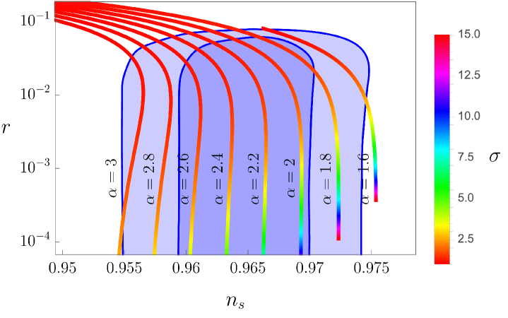
Figure 4: Comparison between the inflationary predictions (83) for $N=60$ and the Planck/BICEP2 data at $1\sigma$ and $2\sigma$ C.L.

4.2 Crossover and infrared regimes

Scale invariance is substantially violated when the coefficient of the kinetic term in Eq. (75) changes from positive to negative values. During this crossover regime rapid variations of the dimensionless couplings in the theory are expected to occur as they transition from their UV to IR fixed-point values. Among other effects, this can play a major role on the onset of the standard hBB era. The minimal heating scenario involves the quantum effective potential for Higgs field $H$,

$$V_{H}=\frac{1}{2}\lambda(\varphi/\mu)\left(H^{\dagger}H-\alpha(\varphi/\mu)\varphi^{2}\right)^{2}\,,$$ (85)

with the dimensionless couplings $\lambda(\varphi/\mu)$ and $\alpha(\varphi/\mu)$ strongly violating the adibaticity condition after the end of inflation and setting to their IR fixed-point values before big bang nucleosynthesis. When written in the Einstein-frame this behaviour leads to interactions of the runaway form (51), allowing to apply the techniques presented in Section 2.3. Alternatively, one could consider a heating stage involving the production of new particles, which should eventually decay into the Standard Model content.

After heating and entropy production, the cosmon field starts to approach the IR fixed point, with a characteristic time scale $\mu$. In the scaling frame (75), the Universe shrinks, while both temperature and particle masses increase with time and the size of atoms decrease [156]. For $\mu^{-1}=10^{10}\,\textrm{yr}=1.2\times 10^{60}M_{P}^{-1}$, the current expectation value of the cosmon field equals the observed reduced Planck mass, $\varphi(t_{0})=2.48\times 10^{18}$ GeV, such that $\varphi/\mu=1.2\times 10^{60}$ [136, 112, 39]. This picture should be understood as equivalent to the standard hBB picture of an expanding and cooling Universe, since the observable dimensionless ratios still coincide with those in the usual scenario. This can be seen explicitly by performing a Weyl redefinition of the metric bringing the action (75) to a canonical form with constant Planck scale and fixed particle masses [116]. This equivalence can be extended to other relevant quantities for cosmology, such as the correlation functions of primordial density fluctuations [157, 158].

Realistic scenarios involve, customarily, a constant or slowly varying form of $B$ following from instance from an IR flow equation with anomalous dimension $\sigma_{\rm IR}$ and small corrections proportional to $B$ [136, 116, 125, 112, 39],

$$\mu\,\partial_{\mu}\ln B=\sigma_{\rm IR}+\kappa\,B\,.$$ (86)

The dominant scaling violation at this time is associated with the potential term $\mu^{2}\varphi^{2}$ in Eq. (75). In particular, the dimensionless ratio of this quantity to the fourth power of the effective Planck mass $\varphi$ decreases with time, reaching very small values at present times. Note also that the enhanced conformal symmetry for $B=\mu=0$ implies that the $\beta$-function for $B$ must vanish at $B=0$. In this limit, $\sigma_{\rm IR}=0$.

Approximate tracking solutions in which the dark energy evolution follows the dominant radiation or matter components have been extensively studied in the literature [116, 136, 125]. These scenarios include generically an additional beyond the Standard Model sector with a late crossover regime able to stop the tracking solution at the present cosmological era. A rather natural setup appears in seesaw [159, 160, 161] and cascade [162, 163, 164] scenarios in which the mass of heavy right-handed neutrinos or scalar triplets decreases with the cosmon field $\varphi$, leading to an increasing neutrino-to-electron mass ratio [165, 166]. In the Einstein frame with fixed electron mass, this reduces to the growing neutrino mass mechanism described in Section (5.1.1).

5 Phenomenology

One of the most crucial aspects in the era of precision cosmology is to gain knowledge on the fundamental mechanisms behind cosmological acceleration while identifying new signatures potentially detectable with present or near future observational campaigns.

In this second part of the review we will discuss the phenomenology associated with quintessential inflation scenarios and the interplay between the cosmon and other fields that might be present in the very early Universe.

5.1 Coupled quintessence

In this type of scenarios the cosmon field is allowed to exchange energy with a given matter component, such as baryons, radiation, cold dark matter or neutrinos. The interaction with baryons and photons is, however, strongly restricted by local gravity measurements [167, 168, 169] and the non-variation of fundamental constants [170], leaving the coupling to dark matter [125, 174, 175, 176, 177, 178, 179, 180, 181, 182] and/or neutrinos [183, 184, 165, 166, 185, 186, 187, 188, 189, 190, 191, 192, 193] as the main viable possibility. This coupling can be formulated either at the level of the equations of motion or at the level of the action.

Heuristic and phenomenological modifications of the equations of motion have been extensively used in the literature, with typical interactions kernels involving local and non-local functions of the relevant energy densities [178, 194, 195, 196, 197, 198], their derivatives [199, 200, 201, 198] and/or a given temporal scale, such as the Hubble parameter [178, 194, 195, 196] or a constant decay rate [196, 202]. These phenomenological approaches are mathematically simple but in many cases physically ill-defined. On the one hand, they usually lack a covariant form for the energy-momentum transfer able to unambiguously describe realistic cosmologies involving perturbations. On the other hand, there is no clear reason for the effective cosmon-matter coupling to be dictated by global properties of the Universe, rather than by purely local ones.

The above problems are avoided in field theory formulations. In particular, cosmon-matter interactions appear naturally in variable and modified gravity scenarios when written in the Einstein frame [203]. To show this, one can consider an initial Jordan-frame action of the form (66) complemented with an exemplary matter action for an uncoupled fermionic field $\psi$ with constant mass $\bar{m}_{\psi}$, 

$$S_{\psi}=\int d^{4}x\sqrt{-g}\left[\frac{i}{2}\left(\bar{\psi}\gamma^{\mu}\nabla_{\mu}\psi-\bar{\psi}\overleftarrow{\nabla}_{\mu}\gamma^{\mu}\psi\right)-\bar{m}_{\psi}\bar{\psi}\psi\right]\,.$$ (87)

Transforming both sectors to the Einstein frame and performing a Weyl rescaling of the spinor $\psi\to\Omega^{3/2}(\phi)\,\psi$ with

$$\Omega^{2}=\frac{f(\phi)}{M_{P}^{2}}\,,\hskip 56.9055pt\left(\frac{d\phi}{d\varphi}\right)^{2}=\frac{3}{2}\left(\frac{\partial\ln f}{\partial\varphi}\right)^{2}+\frac{k}{f}\,,$$ (88)

we get

$$S=\int{\rm d}^{4}x\sqrt{-g}\left[\frac{M^{2}_{\rm P}}{2}R-\frac{1}{2}(\partial\phi)^{2}-V(\phi)+\frac{i}{2}\left(\bar{\psi}\gamma^{\mu}\nabla_{\mu}\psi-\bar{\psi}\overleftarrow{\nabla}_{\mu}\gamma^{\mu}\psi\right)-m_{\psi}(\phi)\bar{\psi}\psi\right]\,\,.$$ (89)

In this representation, the matter field $\psi$ interacts with the cosmon via the $\phi$-dependent mass term

$$m_{\psi}(\phi)\equiv\frac{\bar{m}_{\psi}\,M_{P}}{\sqrt{f(\phi)}}\,.$$ (90)

The variation of the action (89) with respect to the Einstein-frame metric provides the usual Einstein’s equations. The conservation of stress-energy in the presence of the aforementioned energy-momentum exchange can be then written as

$$\nabla_{\nu}T_{\phi}^{\mu\nu}=+\frac{\beta(\phi)}{M_{P}}T_{\psi}\partial^{\mu}\phi\,,\hskip 56.9055pt\nabla_{\nu}T_{\psi}^{\mu\nu}=-\frac{\beta(\phi)}{M_{P}}T_{\psi}\partial^{\mu}\phi\,,$$ (91)

with

$$\beta(\phi)\equiv-M_{P}\frac{\partial\ln m_{\psi}(\phi)}{\partial\phi}\,,$$ (92)

and $T_{\psi}=T_{\psi}^{\mu\nu}g_{\mu\nu}$ the trace of the energy momentum tensor for the $\psi$-field, which vanishes identically for relativistic particles. As anticipated, these expressions are fully covariant and determined by microphysics. The effective coupling $\beta$ modifies equivalently the effective Klein-Gordon equation for the cosmon field

$$\nabla_{\mu}\nabla^{\mu}\phi=V^{\prime}(\phi)+\beta(\phi)T_{\psi}\,,$$ (93)

and the evolution of neutrinos on a classical path [188]

$$\frac{\mathrm{d}u^{\mu}}{\mathrm{d}\tau}+\Gamma^{\mu}_{\rho\sigma}u^{\rho}u^{\sigma}=\beta(\phi)\,u^{\lambda}\partial_{\lambda}\phi\,u^{\mu}+\beta(\phi)\,\partial^{\mu}\phi\,,$$ (94)

with $u^{\mu}$ the four-velocity, $\Gamma_{\mu\nu}$ the Christoffel symbols associated to the metric $g_{\mu\nu}$ and $\tau$ the proper time. The right-hand side of Eq. (94) plays the role of an additional fifth-force and consists of a velocity-dependent piece $\beta(\phi)\,u^{\lambda}\partial_{\lambda}\phi\,u^{\mu}$ ensuring momentum conservation for particles moving in a varying cosmon field and a velocity-independent piece $\beta(\phi)\,\partial^{\mu}\phi$ becoming dominant for small velocities.

In the Einstein frame, a given model within the paradigm is specified by a choice of the effective coupling $\beta(\phi)$. A simple possibility is to consider an effective coupling $\beta(\phi)=-gM_{P}/(m_{0}+g\phi)$ following from a renormalizable Yukawa interaction $m_{\psi}(\phi)\bar{\psi}\psi=m_{0}\bar{\psi}\psi+g\phi\bar{\psi}\psi$, with $m_{0}$ a mass parameter and $g$ a dimensionless coupling. Another option is to consider a setup involving a constant $\beta$ coupling. This describes dilatonic like interactions $m_{\psi}(\phi)\bar{\psi}\psi=m_{0}\exp\left(-\beta\phi/M_{P}\right)\bar{\psi}\psi$ like those appearing in induced and modified gravity scenarios [155, 207, 208]. At the phenomenological level, these choices have been applied in a variety of contexts, ranging from growing neutrino scenarios aiming to solve the coincidence problem [183, 184, 165, 166, 185, 186, 187, 188, 189, 190, 191, 192, 193] to strongly coupled cosmologies [174, 209, 210, 211, 212, 213, 214, 215] inducing the formation of primordial black holes [216, 217, 218, 219] or similar compact objects [220] during radiation domination. In the following sections, we describe these applications in detail.

5.1.1 Growing neutrino masses

Every quintessential inflation model must predict the correct amount of dark energy, preferably without an excessive finetuning of the initial conditions. In this regard, tracking or attractor solutions as those presented in Section 2.4 are particularly interesting, albeit they require an additional exit mechanism able to initiate the current accelerated expansion of the Universe. Growing neutrino quintessence explains the transition from a scaling solution to a dark energy dominated era by identifying the fermion field $\psi$ in Eq. (89) with the neutrino [183, 184, 165, 166, 185, 186, 187, 188, 189, 190, 191, 192, 193]. The special role of this particle can be motivated by a cross-over regime in a beyond the Standard Model sector, manifesting itself in the neutrino masses through a seesaw or cascade mechanism [112], cf. Section 4.

In growing neutrino quintessence, the “why now” problem becomes related to a physical trigger event: the recent change of the effective neutrino equation of state. In particular, when neutrinos become non-relativistic at redshift $z\approx 5$ [185], a negative choice of $\beta$ induces a fixed point in the Klein-Gordon equation (93) for the cosmon field, $-\beta(\phi)\rho_{(\psi)}\simeq-V^{\prime}(\phi)$, effectively stopping its evolution in the runaway potential $V(\phi)$ and pushing it away from the scaling solution. For neutrino masses in the eV (or sub-eV) range, this leads to an almost de Sitter equation of state [166, 165]

$$1+w(t_{0})=\frac{m_{\psi}(t_{0})}{12\,{\rm eV}}\,,$$ (95)

and an energy density roughly matching the observed value $\rho_{\phi}(t_{0})^{1/4}=2\cdot 10^{-3}$ eV,

$$\rho_{\phi}^{1/4}(t_{0})=1.27\left(\frac{\gamma_{\psi}\,m_{\psi}(t_{0})}{{\rm eV}}\right)^{1/4}10^{-3}\,{\rm eV}\,,$$ (96)

with $\gamma_{\psi}=\tilde{\gamma}(t_{0})$ a dimensionless ${\cal O}(1)$ parameter encoding the growth rate of the neutrino mass [166, 165].

Under some circumstances, the long-range interactions mediated by the cosmon can give rise to the formation of dense non-linear neutrino lumps  [185, 187, 221, 189, 222, 223, 188, 190, 191, 192, 193]. The formation of these objects is conceptually similar to that of gravitational structures, being the main differences associated to the field dependent mass $m(\phi)$, which varies both in space and time. The impact of neutrino lumps on large scales depends crucially on the presence or absence of a variation of the effective coupling (92). In the constant coupling model, the instabilities are resolved by the formation of sizable stable lumps typically exceeding the size of large galaxy clusters. The associated backreaction effects lead to the suppression of the (averaged) energy-momentum trace in Eq. (93), weakening the deceleration of the cosmon field and making it difficult to obtain a realistic cosmology [192]. This is due to two effects: i) the acceleration of neutrinos during collapse, which tends to make them relativistic close to the center of the lumps and ii ) the local negative value of the cosmon perturbation $\delta\phi$ within the lumps, which leads to neutrino masses $m_{\psi}(\bar{\phi}+\delta\phi)$ smaller than expected from the average field $\bar{\phi}$ [189]. On the other hand, phenomenologically viable scenarios for variable $\beta$ and small neutrino masses seem a priori plausible [193].

5.1.2 Primordial structure formation

The potential existence of an additional force stronger than gravity in coupled quintessence scenarios opens the possibility of inducing structure formation even in a radiation dominated epoch in which the standard gravitational collapse is inefficient. To this end, the fermion field $\psi$ must be identified with a beyond the Standard Model particle playing the role of dark matter and becoming non-relativistic prior to matter-radiation equality. As shown in Refs. [125, 174, 224, 209, 210, 216], for constant $\beta\gg 1$ and subleading fermion and cosmon components, this scenario admits a scaling solution during radiation domination in which the mass of the fermion decreases with time, $m_{\psi}\sim a^{-1}$, and

$$\phi^{\prime}=\frac{M_{P}}{\beta}\,,\hskip 28.45274pt\Omega_{\psi}=\frac{1}{3\beta^{2}}\,,\hskip 28.45274pt\Omega_{\phi}=\frac{1}{6\beta^{2}}\,,\hskip 28.45274pt\Omega_{R}=1-\frac{1}{2\beta^{2}}\,,$$ (97)

with $\Omega_{\psi},\Omega_{\phi},\Omega_{R}$ the energy density parameters of the $\phi$, $\psi$ and radiation fluids. In the absence of shear or rotational components in the initial velocity field, the density contrast of the $\psi$ field satisfies approximately [174, 209, 210, 216]

$$\delta_{\psi}^{\prime\prime}-\delta_{\psi}^{\prime}-(1+\delta_{\psi})\delta_{\psi}-\frac{4}{3}\frac{\delta_{\psi}^{\prime 2}}{(1+\delta_{\psi})}=0\,.$$ (98)

At early times, this differential equation admits a linearized solution [174, 224, 209, 210, 216]

$$\delta_{\psi}=\delta_{\psi,\rm in}\left(\frac{a}{a_{\rm in}}\right)^{p}\,,\hskip 56.9055ptp=\frac{1}{2}\left(1+\sqrt{5}\right)\,,$$ (99)

with $a_{\rm in}$ the scale factor at the onset of the scaling regime and $\delta_{\psi,\rm in}$ an initial value for the fluctuations which should be determined by requiring compatibility with CMB observations [216].

Depending on the velocity distribution, the rapid growth (99) can lead to the production of primordial black holes [216] or virialized halos which could dominate the dark matter content of the Universe while passing the stringent microlensing constraints and cosmic microwave background energy injection bounds [220]. The formation process of primordial dark matter halos assumes the onset of a screening mechanism at the time of formation. The analysis of this stage is, however, complicated due to the highly non-linear and strong coupling regime of the problem at hand. In particular, most of the equations cannot be consistently linearized without leading to an unbounded growth of perturbations that becomes unphysical at late times. On top of that, the treatment implicitly neglects spatial density and temperature distributions and the potential existence of smaller halos inside larger halos. Consequently, the stability of the lumps can be most probably addressed via $N$-body simulations only. If screening turns out to be inefficient, the long-range forces could potentially cause the emission of scalar waves by accelerated particles, dissipating energy from a halo and making it collapse into black holes [218].

5.2 Hubble-induced phase transitions

In this section we present the phenomenology associated to the interplay between non-minimally coupled spectator fields and a period of kination. Before going into the details, it is worth to discuss the generality of this scenario. On the one hand, non-minimal couplings to gravity are to be expected from quantum field theory calculations on curved space-times [104]. On the other, it is also natural to consider the spectator field to be massive and/or self interacting, including potentially higher-order operators as those generically expected in effective field theories not involving shift symmetry. Additionally, the scalar field could display additional global or local symmetries, being the former potentially broken by gravity [225]. As we shall see, the combination of a long lasting period of kination with the ingredients above leads unavoidably to the spontaneous breaking of the internal symmetry of the spectator field when the background transitions from inflation to kination. This Hubble-induced spontaneous symmetry breaking (SSB) has been considered in the literature as a heating mechanism [226, 227, 101, 102, 103] but also in the context of gravitational waves production [80], Affleck-Dine baryogenesis [54] and dark matter [228, 229, 230].

5.2.1 Spectator field dynamics

To discuss the dynamics of Hubble-induced phase transitions, let us a consider a canonical quintessential scenario like the one in Section 2 supplemented with an exemplary action

$$S_{\chi}=\int d^{4}x\sqrt{-g}\left[-\frac{1}{2}g^{\mu\nu}\partial_{\mu}\chi\partial_{\nu}\chi-\frac{1}{2}\left(m_{\chi}^{2}+\xi R\right)\chi^{2}-V(\chi)\right]$$ (100)

for an energetically-subdominant and non-minimally coupled spectator field $\chi$ with bare mass $m_{\chi}$ and self-interaction potential

$$V(\chi)=\frac{\lambda}{2n}\frac{\chi^{2n}}{\Lambda^{2n-4}}\,,$$ (101)

with $\lambda$ a dimensionless coupling constant and $\Lambda$ an UV suppression scale. For the sake of simplicity we have assumed the spectator field to be real and imposed a discrete $Z_{2}$ symmetry. These restrictions will not play, however, a key role in the following developments, being the phenomenology presented below easily extendable to more general settings and symmetry groups.

From the point of view of the spectator field, the only relevant aspect of the cosmon evolution is the transition from inflation to kinetic domination, with the correspondent change in the equation-of-state parameter from $w=-1$ to $w=+1$. During inflation ($w=1$, $R=12H^{2}$) the effective square mass of the $\chi$ field is large and positive for sufficiently big non-minimal couplings, $\xi\gtrsim 1/12$, locking it at the origin potential and preventing the generation of sizeable isocurvature perturbations in potential conflict with CMB constraints [4]. However, as soon as the background evolution changes from inflation to kination ($w=1$, $R=-6H^{2}$), the origin of the potential becomes a local maximum for small bare masses $m^{2}_{\chi}<6\xi R$, forcing the spectator field to evolve towards the new time-dependent minima appearing at large field values

$$|\chi_{\rm min}|=H\left(\frac{6\xi-m^{2}_{\chi}/H^{2}}{\lambda}\right)^{\frac{1}{2(n-1)}}\left(\frac{\Lambda}{H}\right)^{\frac{n-2}{n-1}}\,.$$ (102)

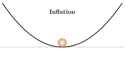
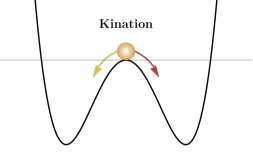
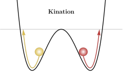
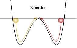
Figure 5: Schematic illustration of the evolution of the spectator field fluctuations during inflation and kination. During inflation the field distribution sits at the minimum of the effective potential. The internal symmetry of the field is, however, spontaneously broken at the onset of kination, forcing the field distribution to evolve towards two new minima appearing at large field values. Due to the time-dependence of the potential, the distribution is not trapped there, but rather oscillates with a bi-modal pattern around the origin.

The transition between the inflationary and kinetic dominated epochs depends on the details of the quintessential inflation potential. If it occurs rapidly, the phase transition can be taken to be almost instantaneous. In other words, the spectator field is not moving away from the inflationary minimum while the potential is changing from the unbroken to the broken phase form. This is typically the situation realized in quintessential inflationary scenarios, where the cosmon potential at the end of inflation is steep. Another important aspect to keep in mind is that the background evolution is assumed to be homogeneous, and hence the transition occurs at the same time everywhere.  Then, at the time of symmetry breaking the field has zero mean $\langle\chi\rangle=0$ and a certain variance $\langle\chi^{2}\rangle$ dictated by vacuum fluctuations. During the broken phase, the effective mass is negative and the system undergoes a stage of tachyonic or spinodal instability, which rapidly amplifies the quantum fluctuations while keeping their zero average value. In particular, the symmetry breaking process is local and any vacua or direction to it is equally probable. Then, the averaged value of the scalar field over scales much larger than the correlation length must identically vanish. This crucial observation implies that any description in terms of a homogeneous spectator field rolling down a potential is inaccurate to start with [231, 232, 233, 103]. This has two major implications. First, the dynamics of the scalar field leads to the generation of temporary topological defects. Second, the energy in gradients is non-negligible and the virialization of the system leads to an asymptotic equation-of-state parameter $w=1/3$, regardless of the specific self-interaction potential (101).

The tachyonic instability, which can be significantly long lasting since the new minima of the effective potential can be quite displaced from the origin and the kination period can last many $e$-folds, ends when the effective mass of the $\chi$ field turns positive. This can occur at the onset of radiation domination, where $R\simeq 0$, or be induced by the higher-order corrections or the bare mass parameter in Eq. (100), provided that these overcome the Ricci scalar contribution at a given time. At this point, the stability is fully restored and the origin becomes again the true minimum of the potential. However, as we shall see below, there is still the possibility that the symmetry restoration is only effectively realized. This peculiar characteristic of Hubble-induced phase transitions occurs when the energy lost by the spectator field in one oscillation is smaller than the flattening of the effective potential minimum, a quantity that can be easily inferred from Eq. (102). In this case, the field distribution is able to pass back the origin of the potential, giving rise to an interacting bimodal distribution that oscillates around it. The other possibility is that the field radiates enough energy as to get trapped in the new minima of the potential at a given time, tracking their subsequent evolution and giving rise to more standard topological defects with time-dependent tension and width [80]. This interesting scenario could be realized, for instance, if the spectator field is allowed to decay into other species or if the effective friction experienced by it is somehow enhanced.

To quantify the above qualitative description, we can rewrite the action (100) in terms of the coordinates and field variables in (36), getting

$$S_{\chi}=\int d^{3}y\,dz\left[\frac{1}{2}(Y^{\prime})^{2}-\frac{1}{2}|\nabla Y|^{2}+\frac{1}{2}M^{2}(z)Y^{2}-\frac{\lambda_{\rm eff}}{2n}Y^{2n}\right]\,,$$ (103)

where the prime denotes derivative with respect to the conformal time $z$,

$$M^{2}(z)=(4\nu^{2}-1)\mathcal{H}^{2}\,,\hskip 56.9055pt\lambda_{\rm eff}=\left(\frac{\chi_{*}}{\Lambda}\frac{a_{\rm kin}}{a}\right)^{2n-4}\,,$$ (104)

and

$$\nu=\sqrt{3\xi/2}\,,\hskip 42.67912pt\mathcal{H}(z)=\frac{1}{2(z+\nu)}\,,\hskip 42.67912pt\mathcal{H}^{\prime}=-2\mathcal{H}^{2}\,,$$ (105)

with the last relation holding during kination. At the onset of this expansion epoch, the spectator field is close to the origin and the higher-order terms in the potential can be safely neglected. This means that the early dynamics of the system can be well described in terms of a free scalar field with a time dependent mass $M^{2}(z)$ and, therefore, exactly solved, as we discussed in Section 5.2.2. In fact, in terms of the dimensionless Fourier mode $\kappa$ in Eq. (36), the problem reduces to find the solutions of the Schrödinger-like differential equation

$$f^{\prime\prime}_{\kappa}+\omega^{2}_{\kappa}(z)f_{\kappa}=0\,,\hskip 56.9055pt\omega_{\kappa}^{2}=\kappa^{2}-M^{2}(z)\,,$$ (106)

for the mode function $f_{\kappa}$ with standard vacuum initial conditions $f_{\kappa}(0)=1/\sqrt{2\kappa}$ and $f^{\prime}_{\kappa}(0)=-i\sqrt{\kappa/2}$. The detailed quantization of the system follows closely the treatment of Refs. [234, 48, 49, 235] and it is detailed for the present case in Ref. [233]. The tachyonic instability induced by kinetic domination amplifies all subhorizon modes within the time-dependent window $\kappa_{\rm min}(z)$ and $\kappa_{\rm max}(z)$, where

$$\kappa_{\rm min}=\mathcal{H}(z)\,,\hskip 56.9055pt\kappa_{\rm max}=(4\nu^{2}-1)^{1/2}\kappa_{\rm min}\,.$$ (107)

The copious production of these modes translates eventually into a quantum-to-classical transition [48, 47, 48, 49, 50, 51], meaning that the properties of the system can be well-approximated by those of a classical random field [233, 103]. In particular, the above system can be solved in terms of Bessel’s functions,

$$f_{\kappa}(z)=\sqrt{z+\nu}\left[A_{\kappa}\mathcal{J}_{\nu}(\kappa(z+\ u))-B_{\kappa}\mathcal{Y}_{\nu}(\kappa(z+\nu))\right]\,,$$ (108)

with $A_{\kappa}$ and $B_{\kappa}$ $\kappa$-dependent coefficients determined by the aforementioned initial conditions. As shown in Fig. 6, the modes that belongs to the unstable region are exponentially amplified. Moreover, one can show that the Heisenberg uncertainty principle in Fourier space can be written as [48, 47, 48, 49, 50, 51, 233, 103]

$$\Delta Y_{\kappa}^{2}\,\Delta\Pi_{\kappa}^{2}=|F_{\kappa}(z)|^{2}+\frac{1}{4}\geq{\frac{1}{4}}\,\Big{|}\langle[Y_{\kappa}(z),\ \Pi^{\dagger}_{\kappa}(z)]\rangle\Big{|}^{2}\,,$$ (109)

with

$$F_{\kappa}(z)={\rm Re}(f^{*}_{\kappa}f^{\prime}_{\kappa})\,,$$ (110)

and the square brackets denoting the anticommutation of the corresponding variables. It is then clear that for $|F_{\kappa}|\gg 1$, the ordering of the operators becomes negligible, as expected for a classical system.

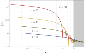
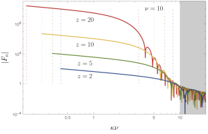
Figure 6: The functions $|f_{\kappa}|$ (left) and $|F_{\kappa}|$ (right) evaluated at different conformal times $z$. The shaded region corresponds to momenta outside the initial amplification band $\kappa>\kappa(z=0)$. The dashed vertical lines corresponds to the time dependent amplification band (107) at the given times.

The above description ceases to be valid as soon as non-linearities kick in. At that moment, in order to properly account for the complete dynamics in the evolution equation

$$Y^{\prime\prime}-\nabla^{2}Y-M^{2}(z)Y+\lambda_{\rm eff}Y^{2n-1}=0\,,$$ (111)

one needs to resort to numerical simulations. Such simulations have been carried out in Ref. [103] for quartic ($n=4$, $\lambda_{\rm eff}=\lambda$) and sextic potentials ($n=6$, $\lambda_{\rm eff}=\lambda(\chi_{*}/\Lambda\,a_{\rm kin}/a)^{4}$). Despite the complexity of the non-linear physics involved, it is still possible to picture the evolution during the broken phase in rather simple terms. As soon as the relevant scales can be treated classically, the field value moves locally towards the new minima, where locally means that the field spatial distribution will look homogeneous on scales smaller than the correlation length $\kappa_{*}=\sqrt{\nu+1}\mathcal{H}(z)$ [233]. This is exactly what is shown in the first three panels of Fig. 7, where we display a few two-dimensional snapshots of the simulation ran in Ref. [103] for a quartic potential. The first box shows the initial classicalized configuration, with the spectator field still very close to the vacuum initial conditions. The second to fourth boxes display the displacement of the spectator field from the origin, growing in amplitude and generating a rather inhomogeneous distribution. Since we are considering a $Z_{2}$ symmetric field, this implies the formation of regions of positive and negative field values separated by domain wall configurations. It is worth noticing that the characteristic scale of the inhomogeneity decreases with time. In particular, the profile of the inhomogeneities is smoother when the field rolls towards the broken phase minima, while it becomes more jagged in the subsequent evolution. This is due to the fact that after the field distribution reaches a minimum and bounces back, it is able to cross the origin towards the opposite minimum. Hence, the spectator field is effectively oscillating in a quartic potential, permitting energy exchange and making the oscillating defects fragment, while they diminish in amplitude and size. Despite this, the energy stored in the gradients of the spectator field is not decreasing with time and it represents a non-negligible fraction of the total field energy density for the total duration of the simulation. This confirms the idea that the Hubble-induced symmetry breaking is an inherently inhomogeneous process.

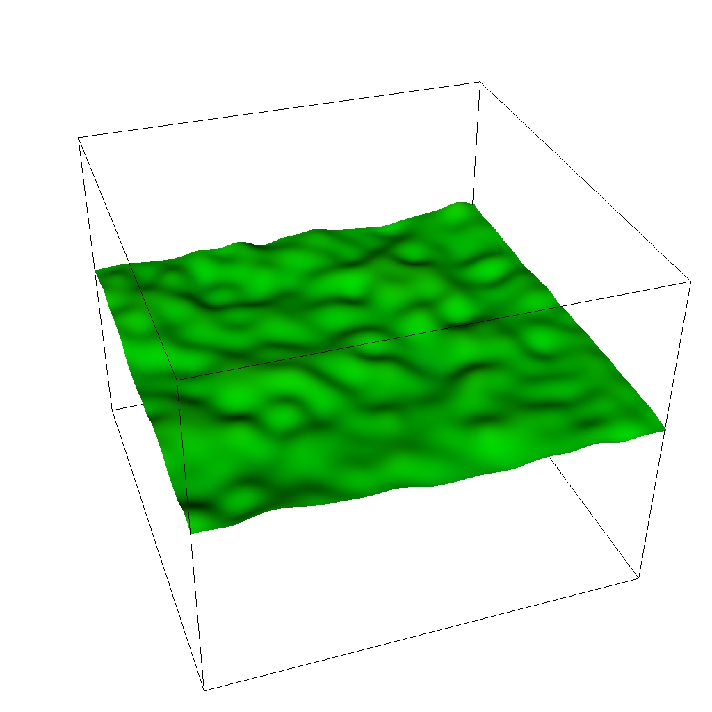
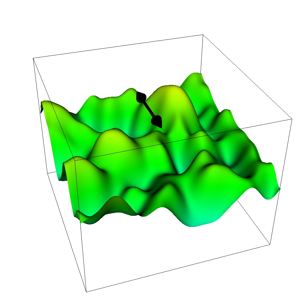
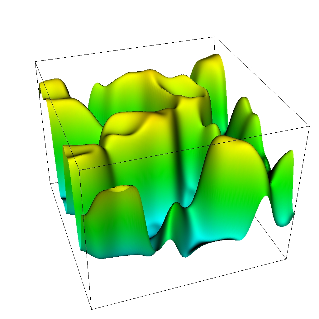
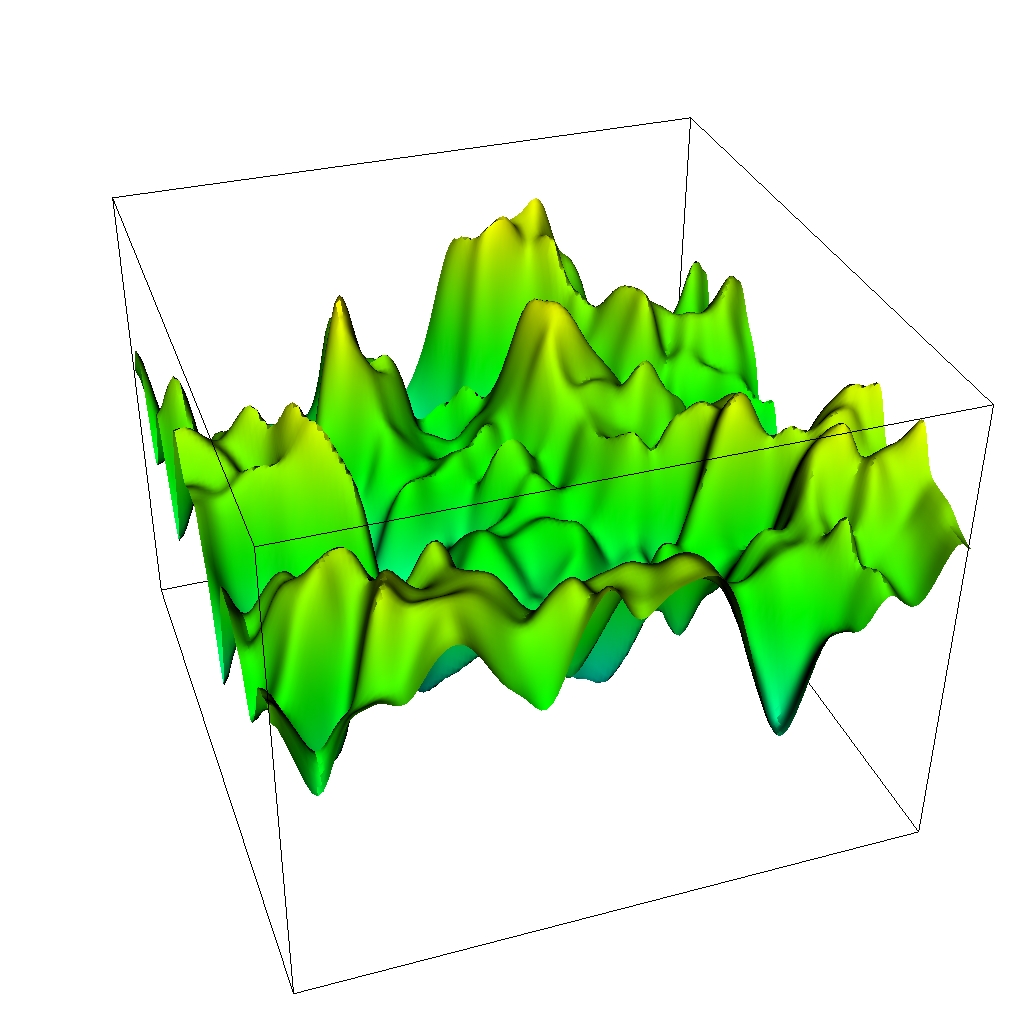
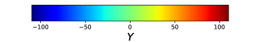
Figure 7: Spectator field growth for the benchmark point $\nu=10$, $\lambda=10^{-4}$. We display 2-dimensional sections of a fraction $V/8$ of the 3-dimensional simulation volume $V$ at times $z=5,\,10,\,15,\,60$, with the $z$-axis indicating the corresponding field value at each point in this surface. The black segment in the second panel indicates the typical scale of the highest peaks. (Images from [103])

5.2.2 Applications

In this last part of the manuscript, we will focus on the expected phenomenology of the above scenario. In particular, we will describe the consequences of inhomogeneities and review some new aspects to be expected when changing the symmetry group or applying this mechanism to dark matter.

Heating

The fast amplification of the the spectator field fluctuations triggered by the Hubble-induced SSB plays an important role when it comes to the heating of the Universe. This can be understood by realizing that the effect of the non-minimal coupling decreases with time, eventually becoming negligible in the determination of the spectator field dynamics. From there on, the field behaves almost as if it were minimally coupled to gravity. In particular, it will tend to virialize, achieving an equation-of-state parameter asymptotically close to the radiation value $w=1/3$. In fact, for monomial potentials like the ones under consideration, the equations-of-state parameter can be written as [236, 237]

$$w_{\chi}=\frac{1}{3}+\frac{2}{3}\frac{(n-2)}{(n+1)+\langle(\nabla\chi/a)^{2}\rangle/\langle V\rangle}\,,$$ (112)

showing clearly that the field will behave as a radiation component provided that the gradients dominate over the potential and independently of the specific higher-order operators involved. For illustration purposes, we display in Fig. 8 the time evolution of the equation-of-state parameter for quartic and sextic potentials. It is worth stressing that if one were to consider the spectator field as a homogeneous condensate the equation of state would be that of radiation only for the first potential, taking the value $w=1/2$ for the sextic one. This crucial difference remarks how crucial inhomogeneities are in the context of SSB.

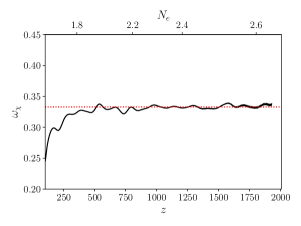
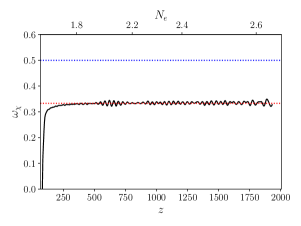
Figure 8: (Left) Evolution of the volume and time averaged equation-of-state parameter (112) for a quartic potential. (Right) Evolution of the same quantity for a sextic potential. The red horizontal line corresponds to the radiation value $1/3$ while the blue line corresponds to the value $1/2$. (Images credit [103])

Another important aspect to keep in mind is that tachyonic instability only amplifies IR modes thus generating an initially far-from-thermal spectrum, as that displayed in Fig. 9. However, the subsequent turbulent evolution of the system induces a slow shift of the spectral peak, which moves gradually towards the UV, leading to eventually a close-to-thermal distribution [106, 107].

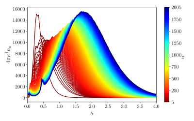
Figure 9: Time evolution of the occupation numbers for $\nu=10$ and $\lambda=10^{-4}$. Different colors correspond to different times, as indicated in the figure. (Image credit [103])

When combined with the fast dilution of the background component discussed in Section 2, this implies that the spectator field will eventually become dominant, starting an epoch of radiation domination and setting the conditions for the onset of the hBB era. Of course, much still remains to be said about this process. One might add, for instance, direct interactions between the spectator field and fermions, like in other heating mechanisms [96, 97, 238, 239, 240, 241, 242], or consider this radiation component as an inert, subdominant and extra radiation contribution (obviously satisfying all observational bounds). Also, if a significant bare mass parameter is allowed, the field could eventually oscillate around a quadratic potential, possibly behaving as dark matter (see below).

Gravitational waves

Another interesting phenomenological aspect related to the presence of defects and inhomogeneities is the associated emission of gravitational waves. Since the distribution of the spectator field after the Hubble-induced phase transition is highly inhomogeneous, the transverse traceless part of its energy momentum tensor will generically be non-vanishing, hence providing a source for GW emission. The production of these tensor modes due Kähler-induced potentials has been considered in supersymmetric extensions of the Standard Model [243] and applied to the present Ricci-based scenario in Ref. [80] for a $U(1)$ symmetric spectator field. Although the generation of gravitational waves from topological defects is a very well-known phenomenon [244, 245, 246], the mechanism at hand possesses striking differences. First, the defects will have a typical size proportional to the Hubble rate $\mathcal{H}$, which makes them ‘fat’, as in the context of axion dark matter [247, 248], and with a time-dependent tension and width, meaning that an exact scaling regime [249, 250] is never achieved. Second, the energy density in GW will be naturally amplified during kinetic domination. Although the precise relevance of these phenomena will ultimately depend on the parameters of the model, they represent nonetheless a generic feature of it, potentially within the reach of forthcoming observational campaigns [251, 252], as shown explicitly in Ref. [80]. Interestingly, the obtained GW spectrum displays also a peaked structure, thus easing its discrimination from foreground signals.

Baryogenesis

The observed asymmetry between matter and anti-matter in the Universe remains one of the biggest mysteries in particle physics. Even if the Standard Model could a priori produce a baryonic asymmetry during the electroweak phase transition [253], the resulting value turns out too small as compared with observations. Traditionally, the amount of asymmetry is encoded in the baryon-to-entropy ratio

$$Y_{B}\equiv\frac{n_{B}}{s}=(0.861\pm 0.008)\times 10^{-10}\,,$$ (113)

where $n_{B}=n_{b}-n_{\bar{b}}$ being $n_{b(\bar{b})}$ the number density of (anti)baryons. One of the most successful proposals to explain this small value of this quantity is the so-called Affleck-Dine mechanism [254, 255], which makes use of a gravity-induced SSB during inflation. Interestingly enough, Hubble-induced phase transitions are able to prompt a post-inflationary Affleck-Dine asymmetry generation if the spectator field $\chi$ is charged under a weakly-broken $B-L$ symmetry [54]. In particular, the change of sign of the Ricci scalar at the onset of kinetic domination breaks spontaneously the $U(1)_{B-L}$ symmetry, making the complex spectator field roll towards the new vacuum manifold of the potential with a certain phase that, at each space point, takes a random value. The additional explicit symmetry breaking requirement provides the charge non-conservation. In the polar representation, $\chi=\tfrac{1}{\sqrt{2}}\rho e^{i\theta}$, the associated symmetry-breaking operators adding to the potential (101) can be written as

$$\delta V=-\epsilon_{0}\Lambda^{4-2n}\rho^{2n}F(\theta,\theta_{0})\,,$$ (114)

with $\epsilon_{0}$ and $\theta_{0}$ the amplitude and phase of a complex symmetry-breaking coefficient $\epsilon=\epsilon_{0}e^{i\theta_{0}}$. A net amount of particles over anti-particles can then be produced

$$a^{3}n_{B-L}(t)=q\epsilon_{0}\Lambda^{4-2n}\int^{t}dt\,a^{3}(t)\rho^{2n}F^{\prime}(\theta,\theta_{0})\,,$$ (115)

where the prime stands here for a derivative with respect to the phase $\theta$ and $n_{B-L}=q\rho^{2}\dot{\theta}$ is the $B-L$ current, being $q$ the associated charge. The quantity $n_{B-L}$ keeps growing until the symmetry is restored. In the case of a quartic operator, corresponding to $n=2$, the produced asymmetry is estimated to be [54]

$$\frac{Y_{B-L}}{10\,{\rm GeV}}=\left(\frac{\Theta}{10^{-4}}\right)^{3/2}\frac{H_{\rm kin}}{10^{7}\,{\rm GeV}}\,,$$ (116)

with $\Theta$ the heating efficiency defined in Eq. (31). As this point, it is important to emphasize a fundamental limitation of the procedure. The net baryonic excess (116) is local, and, therefore, the cosmological evolution will put in causal contact patches with different phase values, leading to a net zero charge on large scales! Albeit not usually emphasized, this problem is common to other post-inflationary mechanisms for the generation of baryon asymmetry, as those considered, for instance, in Refs. [256, 257]. A possible way out is to consider a biased minimum, so that the potential is tilted and a unique global minimum exists, see e.g. [258, 259, 260]. Then, even if initially all spectator phases are equally probable, the dynamical evolution will generate a flux towards the true minimum, thus producing a net global asymmetry [54].

Dark matter

The Hubble-induced SSB has also been explored in the context of primordial dark matter production [261, 228, 229, 230]. In particular, Ref. [228] studied the super-Hubble creation of particles when the post-inflationary Ricci scalar can take negative values. This mechanism was also combined there with a post-inflationary period of kination. By solving the equation for the spectator field (111) at one loop precision, it is found a dark matter abundance

$$\Omega_{\chi}h^{2}=0.078\beta^{3/4}\left(\frac{m}{{\rm GeV}}\right)\left(\frac{H_{\rm rad}}{10^{13}{\rm GeV}}\right)^{3/2}\left(\frac{100}{g_{*,{\rm rad}}}\right)^{1/4}\,.$$ (117)

Here $\beta$ is an $\mathcal{O}(1)$ parameter for $\xi\lesssim 10$ representing the energy density of the produced $\chi$ quanta in units of $H_{\rm kin}$. $m$ is the dark matter bare mass parameter whose value is a priory free. However, upper bounds on the cross section for dark matter interactions obtained from galaxy clusters collisions impose the constraint

$$\frac{m}{{\rm GeV}}>0.027\lambda^{2/3}\,.$$ (118)

This bound is more constraining for larger values of $H_{\rm kin}$ and $\lambda$. However, even when these restrictions are combined with the requirement of avoiding dark matter overproduction, one still finds the very broad range of allowed dark matter masses keV $<m<10^{4}$ GeV [228].

6 Discussion and outlook

Inflation and dark energy are usually understood as two independent epochs in the expansion history of the Universe. In this review, we have described how these accelerated expansion eras can be unified into a quintessential inflation framework in which a single degree of freedom, the cosmon, plays simultaneously the role of the inflaton and of the quintessence field.

The naturalness of quintessential inflation is intimately related to its embedding in a fundamental framework able to produce a large hierarchy of scales without involving unacceptable finetunings. Natural realizations might appear, for instance, in variable gravity scenarios involving UV and IR fixed points where scale symmetry is manifestly realized. On top of that, this paradigm should provide a graceful solution to the “why now” problem, potentially associated with some physical mechanism. In this respect, scaling solutions are able to provide a dark energy density comparable to the dominant matter content in the Universe for an extended period of time, reducing with it the tuning on the initial conditions. A suitable clock signalling the end of this scaling regime is naturally provided by neutrinos, which for sub-eV masses becomes non-relativistic around the same time in which dark energy should start to be dominant.

Probably, the most distinctive phenomenology of quintessential inflation is associated to the unavoidable kinetic dominated regime. This unusual stage induces a relative amplification of all radiation and matter components in the Universe, including the products resulting from the heating stage and any stochastic background of gravitational waves of primordial origin. This can be used to put constraints on some of the theory defining parameters. For instance, the compatibility of the primordial tensor perturbations with BBN imposes bounds on the inflationary scale and the duration of kination, or equivalently, on the efficiency of the heating stage. Additional constraints on these quantities could follow from the spontaneous symmetry of internal symmetries of fields non-minimally coupled to gravity and the associated gravitational wave production. In this review we have discussed the Hubble-induced symmetry breaking of two specific symmetries, namely a global U(1) and a discrete Z₂. However, it is worth stressing that this mechanism applies to any symmetry group, provided the appearance of a time-dependent negative mass parameter in the effective potential leading to new minima with a non-trivial topological structure. Furthermore, the expansion rate may also affect a plethora of particle physics processes in the very early Universe, from the generation of the matter-antimatter asymmetry to the abundance of dark matter relics.

Appendix A Frame-invariant formulation of inflation

In this Appendix, we summarize the frame-invariant formulation of inflation in Refs. [263, 134], to which refer the reader for further details.

The variation of the action (75) with respect to the FLRW metric and the scalar field $\varphi$ provides respectively the Friedmann equations [263],

$$H^{2}=\frac{fU}{3}\left(1-\frac{\epsilon_{H}}{3}+\frac{5\,\kappa_{H}}{3}+\frac{\theta_{H}}{3}\right)^{-1}\,,\hskip 42.67912pt\epsilon_{H}+\kappa_{H}-\theta_{H}=\frac{k\dot{\varphi}^{2}}{2H^{2}f}\,,$$ (119)

and the Klein-Gordon equation

$${\ddot{\varphi}}+(3+\sigma_{H})H{\dot{\varphi}}+\frac{f^{3}}{E}U_{,\varphi}\ =0\,,$$ (120)

with

$$E\equiv kf+\frac{3}{2}f^{2}_{,\varphi}\,,\hskip 56.9055ptU\equiv\frac{V}{f^{2}}\,.$$ (121)

The quantities

$$\epsilon_{H}\equiv-\frac{\dot{H}}{H^{2}}\,,\hskip 42.67912pt\kappa_{H}\equiv\frac{1}{2}\frac{\dot{f}}{Hf}\,,\hskip 42.67912pt\sigma_{H}\equiv\frac{1}{2}\frac{\dot{E}}{HE}\,,\hskip 42.67912pt\theta_{H}\equiv\frac{1}{2}\frac{\ddot{f}}{H^{2}f}\,,$$ (122)

in these expressions can be understood as a generalization of Hubble slow-roll parameters. Assuming these to be small during the inflationary stage, we can rewrite Eqs. (119) and (120) as

$$H^{2}\simeq\frac{fU}{3}\,,\hskip 56.9055pt3H{\dot{\varphi}}\simeq-\frac{f^{3}}{E}U_{,\varphi}\,,$$ (123)

and compute the scalar and tensor power spectra

$$P_{s} \approx \frac{k^{3}}{24\pi^{2}}\,\frac{U}{\epsilon_{U}+\kappa_{U}}\,,\hskip 42.67912ptP_{t}\approx\frac{2k^{3}}{3\pi^{2}}\,U\,,$$ (124)

and the associated spectral tilt and tensor-to-scalar ratio,

$$1-n_{s} = 4\epsilon_{U}+2(\sigma_{U}-\delta_{U}-\kappa_{U})\,,\hskip 42.67912ptr=16(\epsilon_{U}+\kappa_{U})\,,$$ (125)

with

$$\epsilon_{U}\ \equiv \ \frac{1}{2}\,\frac{fU_{,\varphi}(fU)_{,\varphi}}{EU^{2}}\ ,\hskip 28.45274pt\delta_{U}\equiv\frac{1}{2}\,\frac{fU_{,\varphi}(fU)_{,\varphi}}{EU^{2}}+\left(\frac{f^{2}U_{,\varphi}}{EU}\right)_{,\varphi}\,,$$ (126)

$$\kappa_{U} \equiv -\frac{f_{,\varphi}}{2}\,\frac{fU_{,\varphi}}{EU}\,,\hskip 28.45274pt\sigma_{U}\equiv-\frac{1}{2}\,\frac{E_{,\varphi}}{E^{2}}\frac{f^{2}U_{,\varphi}}{U}\,,$$ (127)

the generalization of the potential slow-roll parameters. These expressions are intended to be evaluated at a number of $e$-folds $N=\int H\,dt$, computed out of Eqs. (123),

$$N(\varphi)\ =\ -\int_{\varphi}^{\varphi_{\text{end}}}d\varphi^{\prime}\frac{E(\varphi^{\prime})}{f(\varphi^{\prime})^{2}}\,\frac{U(\varphi^{\prime})}{U(\varphi^{\prime})_{,\varphi^{\prime}}}\,,$$ (128)

with $\varphi_{\text{end}}$ the value of $\varphi$ at the end of inflation, determined by a frame-invariant generalization of the standard condition $\epsilon_{U}=1$,

$$\max(\epsilon_{U}+\kappa_{U},|\epsilon_{U}+\delta_{U}+4\kappa_{U}-\sigma_{U}|)=1\,.$$ (129)

Note that, at the leading order in the slow-roll approximation, the inflationary observables are invariant under the separate action of conformal transformations and field reparametrizations even if the slow-roll parameters are themselves transformed, i.e., $\widetilde{n}_{s}(\tilde{\varphi})=n_{s}(\varphi)$, $\widetilde{r}(\tilde{\varphi})=r(\varphi)$. Also, as written in Eq. (128), the number of $e$-folds is invariant under frame transformations. Consequently, we have $\widetilde{n}_{s}(\widetilde{N})=n_{s}(N)$ and $\widetilde{r}(\widetilde{N})=r(N)$.

Appendix B A workout example of crossover regime

For illustration purposes, we present here a specific flow equation smoothly interpolating between the fixed points considered in the main text and allowing for explicit analytical solutions,

$$\mu\,\partial_{\mu}\ln B=\frac{\kappa\,\sigma B}{\sigma+\kappa\,B^{1/\alpha}}\,.$$ (130)

Using Eq. (128) we get

$$B(\bar{N})=\Big{\{}\frac{\sigma}{\kappa}{\cal W}\left[\frac{\kappa}{\sigma}\left(B_{\rm end}\,e^{2\kappa\bar{N}}\right)^{p}\right]\Big{\}}^{1/p}\,,\hskip 42.67912pt$$ (131)

with

$$\bar{N}=N+c^{p}\,,\hskip 42.67912ptc\equiv B_{\rm end}\left(\frac{\alpha}{2\sigma}\right)^{\frac{1}{p}}\,.$$ (132)

The above expression can be alternatively written as

$$B(\bar{N})=B_{\rm end}\Bigg{\{}\left(\frac{1}{2\,\kappa\,p\,c^{p}}\right){\cal W}\left[2\,\kappa\,p\,c^{p}\,e^{2\,\kappa\,p\,\bar{N}}\right]\Bigg{\}}^{1/p}\,.$$ (133)

The associated form $B(\varphi)$ can be trivially computed out of this expression through the relation

$$\frac{\partial\ln\varphi}{\partial N}=-\frac{2}{B}\,,$$ (134)

getting

$$\ln\left(\frac{\varphi}{m\,e^{-\frac{1}{\sigma}\frac{1}{1-q}}}\right)^{\sigma}=\frac{\sigma}{\kappa}(B^{-1})+\frac{(B^{-1})^{1-q}}{1-q}\,,$$ (135)

where we have chosen the integration constant as $C=m\,e^{-\frac{1}{\sigma}\frac{\alpha}{\alpha-1}}$. This can be alternatively written as

$$\ln\left(\frac{\varphi}{m}\right)^{\sigma}=\frac{\sigma}{\kappa}(B^{-1})+\ln_{q}B^{-1}\,,$$ (136)

with

$$\ln_{q}x=\begin{cases}\ln x\hskip 42.67912pt{\rm if}\hskip 14.22636ptx>0\,\,\&\,\,q=1\,,\\ \frac{x^{1-q}-1}{1-q}\hskip 31.29802pt{\rm if}\hskip 14.22636ptx>0\,\,\&\,\,q\neq 1\,,\\ \textrm{undefined}\hskip 17.07164pt{\rm if}\hskip 14.22636ptx\leq 0\,,\end{cases}$$ (137)

the so-called $q$-logarithm function used by Tsallis in non-extensive statistical mechanics [264]. This function is related to the $q$-exponential

$$e_{q}^{x}=\begin{cases}e^{x}\hskip 147.95433pt{\rm if}\hskip 14.22636ptq=1\,,\\ (1+(1-q)x)^{1/(1-q)}\hskip 62.59605pt{\rm if}\hskip 14.22636ptq\neq 1\,,\,\,\&\,\,1+(1-q)x\geq 0\,,\\ 0\hskip 153.64487pt{\rm if}\hskip 14.22636ptq\neq 1\,,\,\,\&\,\,1+(1-q)x<0\,,\end{cases}$$ (138)

(such that $\exp_{q}(\ln_{q}x)=x$ and $\ln_{q}(\exp_{q}x)=x$) and to the Lambert-Tsallis function, defined as [264]

$${\cal W}_{q}(x)e^{{\cal W}_{q}(x)}=x\,,$$ (139)

and satisfying [264]

$${\cal W}_{q}(x)=\ln_{q}x-_{q}\ln{\cal W}_{q}(x)\,,$$ (140)

with

$$a-_{q}b=\frac{a-b}{1+(1-q)b}\,.$$ (141)

In general, Eq. (136) cannot be inverted. However, some solutions can be found for specific values of $\alpha$, namely

$$\alpha=1/2\,,\hskip 14.22636ptB(\varphi)=\frac{1}{2}\left(1-\log\left(\frac{\varphi}{m}\right)^{\sigma}\right)+\sqrt{\frac{\sigma}{\kappa}+\frac{1}{4}\left(1-\log\left(\frac{\varphi}{m}\right)^{\sigma}\right)^{2}}\,,$$ (142)

$$\alpha=1\,,\hskip 14.22636ptB(\varphi)=\frac{\kappa}{\sigma}\,{\cal W}^{-1}\left[\frac{\sigma}{\kappa}\left(\frac{\varphi}{m}\right)^{\sigma}\right]\,,$$ (143)

$$\alpha=2\,,\hskip 14.22636ptB(\varphi)=\left(\frac{1+\sqrt{1+\frac{\sigma}{\kappa}(2+\ln\left(\frac{\varphi}{m}\right)^{\sigma})}}{2+\ln\left(\frac{\varphi}{m}\right)^{\sigma}}\right)^{2}\,.$$ (144)

The cosmological evolution following from the $\alpha=1$ case has been carefully analyzed in Ref. [39], where we refer the interested reader for further details.

References

- [1] M. Kamionkowski and E.D. Kovetz, The Quest for B Modes from Inflationary Gravitational Waves, Ann. Rev. Astron. Astrophys. 54 (2016) 227 [1510.06042].
- [2] Supernova Cosmology Project collaboration, Discovery of a supernova explosion at half the age of the Universe and its cosmological implications, Nature 391 (1998) 51 [astro-ph/9712212].
- [3] Supernova Search Team collaboration, Observational evidence from supernovae for an accelerating universe and a cosmological constant, Astron. J. 116 (1998) 1009 [astro-ph/9805201].
- [4] Planck collaboration, Planck 2018 results. X. Constraints on inflation, Astron. Astrophys. 641 (2020) A10 [1807.06211].
- [5] BICEP, Keck collaboration, Improved Constraints on Primordial Gravitational Waves using Planck, WMAP, and BICEP/Keck Observations through the 2018 Observing Season, Phys. Rev. Lett. 127 (2021) 151301 [2110.00483].
- [6] 2dFGRS collaboration, The 2dF Galaxy Redshift Survey: The Power spectrum and the matter content of the Universe, Mon. Not. Roy. Astron. Soc. 327 (2001) 1297 [astro-ph/0105252].
- [7] 2dFGRS collaboration, Evidence for a non-zero lambda and a low matter density from a combined analysis of the 2dF Galaxy Redshift Survey and cosmic microwave background anisotropies, Mon. Not. Roy. Astron. Soc. 330 (2002) L29 [astro-ph/0109152].
- [8] SDSS collaboration, Detection of the Baryon Acoustic Peak in the Large-Scale Correlation Function of SDSS Luminous Red Galaxies, Astrophys. J. 633 (2005) 560 [astro-ph/0501171].
- [9] R.D. Peccei, J. Sola and C. Wetterich, Adjusting the Cosmological Constant Dynamically: Cosmons and a New Force Weaker Than Gravity, Phys. Lett. B 195 (1987) 183.
- [10] M. Wali Hossain, R. Myrzakulov, M. Sami and E.N. Saridakis, Unification of inflation and dark energy à la quintessential inflation, Int. J. Mod. Phys. D 24 (2015) 1530014 [1410.6100].
- [11] J. de Haro and L.A. Saló, Analytical and numerical review of Quintessential Inflation, 2108.11144.
- [12] B. Spokoiny, Deflationary universe scenario, Phys. Lett. B315 (1993) 40 [gr-qc/9306008].
- [13] P.J.E. Peebles and A. Vilenkin, Quintessential inflation, Phys. Rev. D59 (1999) 063505 [astro-ph/9810509].
- [14] M. Peloso and F. Rosati, On the construction of quintessential inflation models, JHEP 12 (1999) 026 [hep-ph/9908271].
- [15] K. Dimopoulos and J.W.F. Valle, Modeling quintessential inflation, Astropart. Phys. 18 (2002) 287 [astro-ph/0111417].
- [16] M. Giovannini, Low scale quintessential inflation, Phys. Rev. D 67 (2003) 123512 [hep-ph/0301264].
- [17] P. Brax and J. Martin, Coupling quintessence to inflation in supergravity, Phys. Rev. D71 (2005) 063530 [astro-ph/0502069].
- [18] J.C. Bueno Sanchez and K. Dimopoulos, Trapped Quintessential Inflation, Phys. Lett. B 642 (2006) 294 [hep-th/0605258].
- [19] M.W. Hossain, R. Myrzakulov, M. Sami and E.N. Saridakis, Variable gravity: A suitable framework for quintessential inflation, Phys. Rev. D90 (2014) 023512 [1402.6661].
- [20] A. Agarwal, R. Myrzakulov, M. Sami and N.K. Singh, Quintessential inflation in a thawing realization, Phys. Lett. B770 (2017) 200 [1708.00156].
- [21] S. Ahmad, R. Myrzakulov and M. Sami, Relic gravitational waves from Quintessential Inflation, Phys. Rev. D 96 (2017) 063515 [1705.02133].
- [22] C.-Q. Geng, C.-C. Lee, M. Sami, E.N. Saridakis and A.A. Starobinsky, Observational constraints on successful model of quintessential Inflation, JCAP 1706 (2017) 011 [1705.01329].
- [23] K. Dimopoulos and T. Markkanen, Dark energy as a remnant of inflation and electroweak symmetry breaking, JHEP 01 (2019) 029 [1807.04359].
- [24] K. Dimopoulos, M. Karčiauskas and C. Owen, Quintessential inflation with a trap and axionic dark matter, Phys. Rev. D 100 (2019) 083530 [1907.04676].
- [25] D. Benisty and E.I. Guendelman, Lorentzian Quintessential Inflation, Int. J. Mod. Phys. D 29 (2020) 2042002 [2004.00339].
- [26] D. Benisty and E.I. Guendelman, Quintessential Inflation from Lorentzian Slow Roll, Eur. Phys. J. C 80 (2020) 577 [2006.04129].
- [27] M. Karčiauskas, S. Rusak and A. Saez, Quintessential Inflation and the Non-Linear Effects of the Tachyonic Trapping Mechanism, 2112.11536.
- [28] K. Dimopoulos and L. Donaldson-Wood, Warm quintessential inflation, Phys. Lett. B 796 (2019) 26 [1906.09648].
- [29] B. Feng and M.-z. Li, Curvaton reheating in nonoscillatory inflationary models, Phys. Lett. B 564 (2003) 169 [hep-ph/0212213].
- [30] V. Kamali, M. Motaharfar and R.O. Ramos, Warm brane inflation with an exponential potential: a consistent realization away from the swampland, Phys. Rev. D 101 (2020) 023535 [1910.06796].
- [31] E. Guendelman, R. Herrera, P. Labrana, E. Nissimov and S. Pacheva, Emergent Cosmology, Inflation and Dark Energy, Gen. Rel. Grav. 47 (2015) 10 [1408.5344].
- [32] E.I. Guendelman and R. Herrera, Curvaton reheating mechanism in a scale invariant two measures theory, Gen. Rel. Grav. 48 (2016) 3 [1511.08645].
- [33] Planck collaboration, Planck 2018 results. VI. Cosmological parameters, Astron. Astrophys. 641 (2020) A6 [1807.06209].
- [34] Particle Data Group collaboration, Review of Particle Physics, PTEP 2020 (2020) 083C01.
- [35] T. Chiba, A. De Felice and S. Tsujikawa, Observational constraints on quintessence: thawing, tracker, and scaling models, Phys. Rev. D87 (2013) 083505 [1210.3859].
- [36] C.-Q. Geng, M.W. Hossain, R. Myrzakulov, M. Sami and E.N. Saridakis, Quintessential inflation with canonical and noncanonical scalar fields and Planck 2015 results, Phys. Rev. D 92 (2015) 023522 [1502.03597].
- [37] J.-B. Durrive, J. Ooba, K. Ichiki and N. Sugiyama, Updated observational constraints on quintessence dark energy models, Phys. Rev. D 97 (2018) 043503 [1801.09446].
- [38] D.S. Salopek and J.R. Bond, Nonlinear evolution of long wavelength metric fluctuations in inflationary models, Phys. Rev. D 42 (1990) 3936.
- [39] J. Rubio and C. Wetterich, Emergent scale symmetry: Connecting inflation and dark energy, Phys. Rev. D96 (2017) 063509 [1705.00552].
- [40] K. Dimopoulos and C. Owen, Quintessential Inflation with -attractors, JCAP 1706 (2017) 027 [1703.00305].
- [41] Y. Akrami, R. Kallosh, A. Linde and V. Vardanyan, Dark energy, -attractors, and large-scale structure surveys, JCAP 1806 (2018) 041 [1712.09693].
- [42] V.F. Mukhanov and G.V. Chibisov, Quantum Fluctuations and a Nonsingular Universe, JETP Lett. 33 (1981) 532.
- [43] A.H. Guth and S.Y. Pi, Fluctuations in the New Inflationary Universe, Phys. Rev. Lett. 49 (1982) 1110.
- [44] A.A. Starobinsky, Dynamics of Phase Transition in the New Inflationary Universe Scenario and Generation of Perturbations, Phys. Lett. B 117 (1982) 175.
- [45] S.W. Hawking, The Development of Irregularities in a Single Bubble Inflationary Universe, Phys. Lett. B 115 (1982) 295.
- [46] J.M. Bardeen, P.J. Steinhardt and M.S. Turner, Spontaneous Creation of Almost Scale - Free Density Perturbations in an Inflationary Universe, Phys. Rev. D 28 (1983) 679.
- [47] J. Lesgourgues, D. Polarski and A.A. Starobinsky, Quantum to classical transition of cosmological perturbations for nonvacuum initial states, Nucl. Phys. B 497 (1997) 479 [gr-qc/9611019].
- [48] D. Polarski and A.A. Starobinsky, Semiclassicality and decoherence of cosmological perturbations, Class. Quant. Grav. 13 (1996) 377 [gr-qc/9504030].
- [49] C. Kiefer, D. Polarski and A.A. Starobinsky, Quantum to classical transition for fluctuations in the early universe, Int. J. Mod. Phys. D 7 (1998) 455 [gr-qc/9802003].
- [50] C. Kiefer, J. Lesgourgues, D. Polarski and A.A. Starobinsky, The Coherence of primordial fluctuations produced during inflation, Class. Quant. Grav. 15 (1998) L67 [gr-qc/9806066].
- [51] C. Kiefer and D. Polarski, Emergence of classicality for primordial fluctuations: Concepts and analogies, Annalen Phys. 7 (1998) 137 [gr-qc/9805014].
- [52] M. Joyce, Electroweak Baryogenesis and the Expansion Rate of the Universe, Phys. Rev. D 55 (1997) 1875 [hep-ph/9606223].
- [53] M. Joyce and T. Prokopec, Turning around the sphaleron bound: Electroweak baryogenesis in an alternative postinflationary cosmology, Phys. Rev. D 57 (1998) 6022 [hep-ph/9709320].
- [54] D. Bettoni and J. Rubio, Quintessential Affleck-Dine baryogenesis with non-minimal couplings, Phys. Lett. B 784 (2018) 122 [1805.02669].
- [55] M. Kamionkowski and M.S. Turner, THERMAL RELICS: DO WE KNOW THEIR ABUNDANCES?, Phys. Rev. D 42 (1990) 3310.
- [56] P. Salati, Quintessence and the relic density of neutralinos, Phys. Lett. B 571 (2003) 121 [astro-ph/0207396].
- [57] S. Profumo and P. Ullio, SUSY dark matter and quintessence, JCAP 11 (2003) 006 [hep-ph/0309220].
- [58] D.J.H. Chung, L.L. Everett and K.T. Matchev, Inflationary cosmology connecting dark energy and dark matter, Phys. Rev. D 76 (2007) 103530 [0704.3285].
- [59] L. Visinelli and P. Gondolo, Axion cold dark matter in non-standard cosmologies, Phys. Rev. D 81 (2010) 063508 [0912.0015].
- [60] K. Redmond and A.L. Erickcek, New Constraints on Dark Matter Production during Kination, Phys. Rev. D 96 (2017) 043511 [1704.01056].
- [61] F. D’Eramo, N. Fernandez and S. Profumo, When the Universe Expands Too Fast: Relentless Dark Matter, JCAP 05 (2017) 012 [1703.04793].
- [62] F. D’Eramo, N. Fernandez and S. Profumo, Dark Matter Freeze-in Production in Fast-Expanding Universes, JCAP 02 (2018) 046 [1712.07453].
- [63] L. Visinelli, (Non-)thermal production of WIMPs during kination, Symmetry 10 (2018) 546 [1710.11006].
- [64] N. Bernal, J. Rubio and H. Veermäe, Boosting Ultraviolet Freeze-in in NO Models, JCAP 06 (2020) 047 [2004.13706].
- [65] M. Giovannini, Gravitational waves constraints on postinflationary phases stiffer than radiation, Phys. Rev. D 58 (1998) 083504 [hep-ph/9806329].
- [66] M. Giovannini, Production and detection of relic gravitons in quintessential inflationary models, Phys. Rev. D 60 (1999) 123511 [astro-ph/9903004].
- [67] H. Tashiro, T. Chiba and M. Sasaki, Reheating after quintessential inflation and gravitational waves, Class. Quant. Grav. 21 (2004) 1761 [gr-qc/0307068].
- [68] C. Caprini and D.G. Figueroa, Cosmological Backgrounds of Gravitational Waves, Class. Quant. Grav. 35 (2018) 163001 [1801.04268].
- [69] D.G. Figueroa and E.H. Tanin, Inconsistency of an inflationary sector coupled only to Einstein gravity, JCAP 10 (2019) 050 [1811.04093].
- [70] D.G. Figueroa and E.H. Tanin, Ability of LIGO and LISA to probe the equation of state of the early Universe, JCAP 08 (2019) 011 [1905.11960].
- [71] N. Bernal and F. Hajkarim, Primordial Gravitational Waves in Nonstandard Cosmologies, Phys. Rev. D 100 (2019) 063502 [1905.10410].
- [72] S.Y. Khlebnikov and I.I. Tkachev, Relic gravitational waves produced after preheating, Phys. Rev. D 56 (1997) 653 [hep-ph/9701423].
- [73] R. Easther and E.A. Lim, Stochastic gravitational wave production after inflation, JCAP 04 (2006) 010 [astro-ph/0601617].
- [74] R. Easther, J.T. Giblin, Jr. and E.A. Lim, Gravitational Wave Production At The End Of Inflation, Phys. Rev. Lett. 99 (2007) 221301 [astro-ph/0612294].
- [75] J.F. Dufaux, A. Bergman, G.N. Felder, L. Kofman and J.-P. Uzan, Theory and Numerics of Gravitational Waves from Preheating after Inflation, Phys. Rev. D 76 (2007) 123517 [0707.0875].
- [76] J. Garcia-Bellido and D.G. Figueroa, A stochastic background of gravitational waves from hybrid preheating, Phys. Rev. Lett. 98 (2007) 061302 [astro-ph/0701014].
- [77] J. Garcia-Bellido, D.G. Figueroa and A. Sastre, A Gravitational Wave Background from Reheating after Hybrid Inflation, Phys. Rev. D 77 (2008) 043517 [0707.0839].
- [78] Y. Cui, M. Lewicki, D.E. Morrissey and J.D. Wells, Cosmic Archaeology with Gravitational Waves from Cosmic Strings, Phys. Rev. D 97 (2018) 123505 [1711.03104].
- [79] Y. Cui, M. Lewicki, D.E. Morrissey and J.D. Wells, Probing the pre-BBN universe with gravitational waves from cosmic strings, JHEP 01 (2019) 081 [1808.08968].
- [80] D. Bettoni, G. Domènech and J. Rubio, Gravitational waves from global cosmic strings in quintessential inflation, JCAP 02 (2019) 034 [1810.11117].
- [81] C.-F. Chang and Y. Cui, Stochastic Gravitational Wave Background from Global Cosmic Strings, Phys. Dark Univ. 29 (2020) 100604 [1910.04781].
- [82] Y. Gouttenoire, G. Servant and P. Simakachorn, BSM with Cosmic Strings: Heavy, up to EeV mass, Unstable Particles, JCAP 07 (2020) 016 [1912.03245].
- [83] C.-F. Chang and Y. Cui, Gravitational Waves from Global Cosmic Strings and Cosmic Archaeology, 2106.09746.
- [84] D.J.H. Chung and P. Zhou, Gravity Waves as a Probe of Hubble Expansion Rate During An Electroweak Scale Phase Transition, Phys. Rev. D 82 (2010) 024027 [1003.2462].
- [85] R. Allahverdi et al., The First Three Seconds: a Review of Possible Expansion Histories of the Early Universe, 2006.16182.
- [86] M. Maggiore, Gravitational wave experiments and early universe cosmology, Phys. Rept. 331 (2000) 283 [gr-qc/9909001].
- [87] G. Mangano, G. Miele, S. Pastor, T. Pinto, O. Pisanti and P.D. Serpico, Relic neutrino decoupling including flavor oscillations, Nucl. Phys. B 729 (2005) 221 [hep-ph/0506164].
- [88] R.H. Cyburt, B.D. Fields, K.A. Olive and T.-H. Yeh, Big Bang Nucleosynthesis: 2015, Rev. Mod. Phys. 88 (2016) 015004 [1505.01076].
- [89] Y. Gouttenoire, G. Servant and P. Simakachorn, Kination cosmology from scalar fields and gravitational-wave signatures, 2111.01150.
- [90] B.A. Bassett, S. Tsujikawa and D. Wands, Inflation dynamics and reheating, Rev. Mod. Phys. 78 (2006) 537 [astro-ph/0507632].
- [91] R. Allahverdi, R. Brandenberger, F.-Y. Cyr-Racine and A. Mazumdar, Reheating in Inflationary Cosmology: Theory and Applications, Ann. Rev. Nucl. Part. Sci. 60 (2010) 27 [1001.2600].
- [92] L. Kofman, A.D. Linde and A.A. Starobinsky, Towards the theory of reheating after inflation, Phys. Rev. D 56 (1997) 3258 [hep-ph/9704452].
- [93] L.H. Ford, Gravitational Particle Creation and Inflation, Phys. Rev. D 35 (1987) 2955.
- [94] Planck collaboration, Planck 2015 results. XX. Constraints on inflation, Astron. Astrophys. 594 (2016) A20 [1502.02114].
- [95] E.J. Chun, S. Scopel and I. Zaballa, Gravitational reheating in quintessential inflation, JCAP 07 (2009) 022 [0904.0675].
- [96] G.N. Felder, L. Kofman and A.D. Linde, Instant preheating, Phys. Rev. D 59 (1999) 123523 [hep-ph/9812289].
- [97] G.N. Felder, L. Kofman and A.D. Linde, Inflation and preheating in NO models, Phys. Rev. D 60 (1999) 103505 [hep-ph/9903350].
- [98] A.H. Campos, H.C. Reis and R. Rosenfeld, Preheating in quintessential inflation, Phys. Lett. B 575 (2003) 151 [hep-ph/0210152].
- [99] K. Dimopoulos, L. Donaldson Wood and C. Owen, Instant preheating in quintessential inflation with -attractors, Phys. Rev. D 97 (2018) 063525 [1712.01760].
- [100] J.C. Bueno Sanchez and K. Dimopoulos, Curvaton reheating allows TeV Hubble scale in NO inflation, JCAP 11 (2007) 007 [0707.3967].
- [101] K. Dimopoulos and T. Markkanen, Non-minimal gravitational reheating during kination, JCAP 06 (2018) 021 [1803.07399].
- [102] T. Opferkuch, P. Schwaller and B.A. Stefanek, Ricci Reheating, JCAP 07 (2019) 016 [1905.06823].
- [103] D. Bettoni, A. Lopez-Eiguren and J. Rubio, Hubble-induced phase transitions on the lattice with applications to Ricci reheating, 2107.09671.
- [104] N.D. Birrell and P.C.W. Davies, Quantum Fields in Curved Space, Cambridge Monographs on Mathematical Physics, Cambridge Univ. Press, Cambridge, UK (2, 1984), 10.1017/CBO9780511622632.
- [105] V. Mukhanov and S. Winitzki, Introduction to quantum effects in gravity, Cambridge University Press (6, 2007).
- [106] R. Micha and I.I. Tkachev, Relativistic turbulence: A Long way from preheating to equilibrium, Phys. Rev. Lett. 90 (2003) 121301 [hep-ph/0210202].
- [107] R. Micha and I.I. Tkachev, Turbulent thermalization, Phys. Rev. D 70 (2004) 043538 [hep-ph/0403101].
- [108] T. Damour and A. Vilenkin, String theory and inflation, Phys. Rev. D 53 (1996) 2981 [hep-th/9503149].
- [109] J. Haro, Different reheating mechanisms in quintessence inflation, Phys. Rev. D 99 (2019) 043510 [1807.07367].
- [110] J. Haro, W. Yang and S. Pan, Reheating in quintessential inflation via gravitational production of heavy massive particles: A detailed analysis, JCAP 01 (2019) 023 [1811.07371].
- [111] L.A. Saló and J. de Haro, Gravitational particle production of superheavy massive particles in Quintessential Inflation: A numerical analysis, 2108.10795.
- [112] C. Wetterich, Inflation, quintessence, and the origin of mass, Nucl. Phys. B 897 (2015) 111 [1408.0156].
- [113] C. Wetterich, Cosmology with varying scales and couplings, in Proceedings, 5th Internationa Conference on Strong and Electroweak Matter (SEWM 2002): Heidelberg, Germany, October 2-5, 2002, pp. 230–249, 2003, DOI [hep-ph/0302116].
- [114] R.J. Scherrer and A.A. Sen, Thawing quintessence with a nearly flat potential, Phys. Rev. D77 (2008) 083515 [0712.3450].
- [115] R.R. Caldwell and E.V. Linder, The Limits of quintessence, Phys. Rev. Lett. 95 (2005) 141301 [astro-ph/0505494].
- [116] C. Wetterich, Cosmology and the Fate of Dilatation Symmetry, Nucl. Phys. B302 (1988) 668 [1711.03844].
- [117] E.J. Copeland, A.R. Liddle and D. Wands, Exponential potentials and cosmological scaling solutions, Phys. Rev. D57 (1998) 4686 [gr-qc/9711068].
- [118] P.G. Ferreira and M. Joyce, Cosmology with a primordial scaling field, Phys. Rev. D58 (1998) 023503 [astro-ph/9711102].
- [119] S. Casas, M. Pauly and J. Rubio, Higgs-dilaton cosmology: An inflation–dark-energy connection and forecasts for future galaxy surveys, Phys. Rev. D97 (2018) 043520 [1712.04956].
- [120] S. Dutta and R.J. Scherrer, Hilltop Quintessence, Phys. Rev. D 78 (2008) 123525 [0809.4441].
- [121] T. Chiba, Slow-Roll Thawing Quintessence, Phys. Rev. D 79 (2009) 083517 [0902.4037].
- [122] I. Zlatev, L.-M. Wang and P.J. Steinhardt, Quintessence, cosmic coincidence, and the cosmological constant, Phys. Rev. Lett. 82 (1999) 896 [astro-ph/9807002].
- [123] P.J. Steinhardt, L.-M. Wang and I. Zlatev, Cosmological tracking solutions, Phys. Rev. D 59 (1999) 123504 [astro-ph/9812313].
- [124] T. Chiba, The Equation of State of Tracker Fields, Phys. Rev. D 81 (2010) 023515 [0909.4365].
- [125] C. Wetterich, The Cosmon model for an asymptotically vanishing time dependent cosmological ’constant’, Astron. Astrophys. 301 (1995) 321 [hep-th/9408025].
- [126] B. Ratra and P.J.E. Peebles, Cosmological Consequences of a Rolling Homogeneous Scalar Field, Phys. Rev. D37 (1988) 3406.
- [127] T. Barreiro, E.J. Copeland and N.J. Nunes, Quintessence arising from exponential potentials, Phys. Rev. D 61 (2000) 127301 [astro-ph/9910214].
- [128] P.-Y. Wang, C.-W. Chen and P. Chen, Confronting Tracker Field Quintessence with Data, JCAP 02 (2012) 016 [1108.1424].
- [129] S. Tsujikawa, Quintessence: A Review, Class. Quant. Grav. 30 (2013) 214003 [1304.1961].
- [130] D. Langlois, Dark energy and modified gravity in degenerate higher-order scalar–tensor (DHOST) theories: A review, Int. J. Mod. Phys. D 28 (2019) 1942006 [1811.06271].
- [131] T.P. Sotiriou and V. Faraoni, f(R) Theories Of Gravity, Rev. Mod. Phys. 82 (2010) 451 [0805.1726].
- [132] E.E. Flanagan, The Conformal frame freedom in theories of gravitation, Class. Quant. Grav. 21 (2004) 3817 [gr-qc/0403063].
- [133] L. Järv, P. Kuusk, M. Saal and O. Vilson, Invariant quantities in the scalar-tensor theories of gravitation, Phys. Rev. D 91 (2015) 024041 [1411.1947].
- [134] D. Burns, S. Karamitsos and A. Pilaftsis, Frame-Covariant Formulation of Inflation in Scalar-Curvature Theories, Nucl. Phys. B 907 (2016) 785 [1603.03730].
- [135] C. Wetterich, Cosmon inflation, Phys. Lett. B 726 (2013) 15 [1303.4700].
- [136] C. Wetterich, Variable gravity Universe, Phys. Rev. D 89 (2014) 024005 [1308.1019].
- [137] A. Hebecker and C. Wetterich, Natural quintessence?, Phys. Lett. B 497 (2001) 281 [hep-ph/0008205].
- [138] C. Wetterich, Quantum scale symmetry, 1901.04741.
- [139] C. García-García, E.V. Linder, P. Ruíz-Lapuente and M. Zumalacárregui, Dark energy from -attractors: phenomenology and observational constraints, JCAP 1808 (2018) 022 [1803.00661].
- [140] E. Palti, The Swampland: Introduction and Review, Fortsch. Phys. 67 (2019) 1900037 [1903.06239].
- [141] R. Kallosh, A. Linde and D. Roest, Universal Attractor for Inflation at Strong Coupling, Phys. Rev. Lett. 112 (2014) 011303 [1310.3950].
- [142] K. Dimopoulos and S. Sánchez López, Quintessential inflation in Palatini gravity, Phys. Rev. D 103 (2021) 043533 [2012.06831].
- [143] T. Henz, J.M. Pawlowski, A. Rodigast and C. Wetterich, Dilaton Quantum Gravity, Phys. Lett. B 727 (2013) 298 [1304.7743].
- [144] C. Wetterich, Graviton fluctuations erase the cosmological constant, Phys. Lett. B 773 (2017) 6 [1704.08040].
- [145] M.A. Luty, J. Polchinski and R. Rattazzi, The -theorem and the Asymptotics of 4D Quantum Field Theory, JHEP 01 (2013) 152 [1204.5221].
- [146] A. Dymarsky, Z. Komargodski, A. Schwimmer and S. Theisen, On Scale and Conformal Invariance in Four Dimensions, JHEP 10 (2015) 171 [1309.2921].
- [147] C. Wetterich, Eternal Universe, Phys. Rev. D 90 (2014) 043520 [1404.0535].
- [148] E.G. Adelberger, J.H. Gundlach, B.R. Heckel, S. Hoedl and S. Schlamminger, Torsion balance experiments: A low-energy frontier of particle physics, Prog. Part. Nucl. Phys. 62 (2009) 102.
- [149] J.-P. Uzan, Varying Constants, Gravitation and Cosmology, Living Rev. Rel. 14 (2011) 2 [1009.5514].
- [150] M. Shaposhnikov and D. Zenhausern, Scale invariance, unimodular gravity and dark energy, Phys. Lett. B671 (2009) 187 [0809.3395].
- [151] J. Garcia-Bellido, J. Rubio, M. Shaposhnikov and D. Zenhausern, Higgs-Dilaton Cosmology: From the Early to the Late Universe, Phys. Rev. D 84 (2011) 123504 [1107.2163].
- [152] P.G. Ferreira, C.T. Hill and G.G. Ross, No fifth force in a scale invariant universe, Phys. Rev. D95 (2017) 064038 [1612.03157].
- [153] C. Burrage, E.J. Copeland, P. Millington and M. Spannowsky, Fifth forces, Higgs portals and broken scale invariance, 1804.07180.
- [154] S. Casas, G.K. Karananas, M. Pauly and J. Rubio, Scale-invariant alternatives to general relativity. III. The inflation-dark energy connection, Phys. Rev. D99 (2019) 063512 [1811.05984].
- [155] A. Zee, A Broken Symmetric Theory of Gravity, Phys. Rev. Lett. 42 (1979) 417.
- [156] C. Wetterich, Universe without expansion, Phys. Dark Univ. 2 (2013) 184 [1303.6878].
- [157] C. Wetterich, Primordial cosmic fluctuations for variable gravity, JCAP 05 (2016) 041 [1511.03530].
- [158] A. Karam, T. Pappas and K. Tamvakis, Frame-dependence of higher-order inflationary observables in scalar-tensor theories, Phys. Rev. D 96 (2017) 064036 [1707.00984].
- [159] P. Minkowski, at a Rate of One Out of Muon Decays?, Phys. Lett. B 67 (1977) 421.
- [160] T. Yanagida, Horizontal gauge symmetry and masses of neutrinos, Conf. Proc. C 7902131 (1979) 95.
- [161] M. Gell-Mann, P. Ramond and R. Slansky, Complex Spinors and Unified Theories, Conf. Proc. C 790927 (1979) 315 [1306.4669].
- [162] M. Magg and C. Wetterich, Neutrino Mass Problem and Gauge Hierarchy, Phys. Lett. B 94 (1980) 61.
- [163] G. Lazarides, Q. Shafi and C. Wetterich, Proton Lifetime and Fermion Masses in an SO(10) Model, Nucl. Phys. B 181 (1981) 287.
- [164] R.N. Mohapatra and G. Senjanovic, Neutrino Masses and Mixings in Gauge Models with Spontaneous Parity Violation, Phys. Rev. D 23 (1981) 165.
- [165] C. Wetterich, Growing neutrinos and cosmological selection, Phys. Lett. B 655 (2007) 201 [0706.4427].
- [166] L. Amendola, M. Baldi and C. Wetterich, Quintessence cosmologies with a growing matter component, Phys. Rev. D 78 (2008) 023015 [0706.3064].
- [167] C.M. Will, The Confrontation between general relativity and experiment, Living Rev. Rel. 9 (2006) 3 [gr-qc/0510072].
- [168] B. Elder, V. Vardanyan, Y. Akrami, P. Brax, A.-C. Davis and R.S. Decca, Classical symmetron force in Casimir experiments, Phys. Rev. D 101 (2020) 064065 [1912.10015].
- [169] P. Brax, A.-C. Davis, B. Elder and L.K. Wong, Constraining screened fifth forces with the electron magnetic moment, Phys. Rev. D 97 (2018) 084050 [1802.05545].
- [170] J.-P. Uzan, The Fundamental Constants and Their Variation: Observational Status and Theoretical Motivations, Rev. Mod. Phys. 75 (2003) 403 [hep-ph/0205340].
- [171] T. Clifton, P.G. Ferreira, A. Padilla and C. Skordis, Modified Gravity and Cosmology, Phys. Rept. 513 (2012) 1 [1106.2476].
- [172] M. Ishak, Testing General Relativity in Cosmology, Living Rev. Rel. 22 (2019) 1 [1806.10122].
- [173] A. Joyce, B. Jain, J. Khoury and M. Trodden, Beyond the Cosmological Standard Model, Phys. Rept. 568 (2015) 1 [1407.0059].
- [174] L. Amendola, Coupled quintessence, Phys. Rev. D 62 (2000) 043511 [astro-ph/9908023].
- [175] G.R. Farrar and P.J.E. Peebles, Interacting dark matter and dark energy, Astrophys. J. 604 (2004) 1 [astro-ph/0307316].
- [176] L. Amendola, Linear and non-linear perturbations in dark energy models, Phys. Rev. D 69 (2004) 103524 [astro-ph/0311175].
- [177] T. Koivisto, Growth of perturbations in dark matter coupled with quintessence, Phys. Rev. D 72 (2005) 043516 [astro-ph/0504571].
- [178] L. Amendola, G. Camargo Campos and R. Rosenfeld, Consequences of dark matter-dark energy interaction on cosmological parameters derived from SNIa data, Phys. Rev. D 75 (2007) 083506 [astro-ph/0610806].
- [179] C.G. Boehmer, G. Caldera-Cabral, R. Lazkoz and R. Maartens, Dynamics of dark energy with a coupling to dark matter, Phys. Rev. D 78 (2008) 023505 [0801.1565].
- [180] M. Baldi, V. Pettorino, G. Robbers and V. Springel, Hydrodynamical N-body simulations of coupled dark energy cosmologies, Mon. Not. Roy. Astron. Soc. 403 (2010) 1684 [0812.3901].
- [181] M. Baldi, Time dependent couplings in the dark sector: from background evolution to nonlinear structure formation, Mon. Not. Roy. Astron. Soc. 411 (2011) 1077 [1005.2188].
- [182] J. Gleyzes, D. Langlois, M. Mancarella and F. Vernizzi, Effective Theory of Interacting Dark Energy, JCAP 08 (2015) 054 [1504.05481].
- [183] R. Fardon, A.E. Nelson and N. Weiner, Dark energy from mass varying neutrinos, JCAP 10 (2004) 005 [astro-ph/0309800].
- [184] A.W. Brookfield, C. van de Bruck, D.F. Mota and D. Tocchini-Valentini, Cosmology of mass-varying neutrinos driven by quintessence: theory and observations, Phys. Rev. D 73 (2006) 083515 [astro-ph/0512367].
- [185] D.F. Mota, V. Pettorino, G. Robbers and C. Wetterich, Neutrino clustering in growing neutrino quintessence, Phys. Lett. B 663 (2008) 160 [0802.1515].
- [186] V. Pettorino, D.F. Mota, G. Robbers and C. Wetterich, Clustering in growing neutrino cosmologies, AIP Conf. Proc. 1115 (2009) 291 [0901.1239].
- [187] N. Wintergerst, V. Pettorino, D.F. Mota and C. Wetterich, Very large scale structures in growing neutrino quintessence, Phys. Rev. D 81 (2010) 063525 [0910.4985].
- [188] Y. Ayaita, M. Weber and C. Wetterich, Structure Formation and Backreaction in Growing Neutrino Quintessence, Phys. Rev. D 85 (2012) 123010 [1112.4762].
- [189] N.J. Nunes, L. Schrempp and C. Wetterich, Mass freezing in growing neutrino quintessence, Phys. Rev. D 83 (2011) 083523 [1102.1664].
- [190] Y. Ayaita, M. Weber and C. Wetterich, Neutrino lump fluid in growing neutrino quintessence, Phys. Rev. D 87 (2013) 043519 [1211.6589].
- [191] Y. Ayaita, M. Baldi, F. Führer, E. Puchwein and C. Wetterich, Nonlinear growing neutrino cosmology, Phys. Rev. D 93 (2016) 063511 [1407.8414].
- [192] F. Führer and C. Wetterich, Backreaction in Growing Neutrino Quintessence, Phys. Rev. D 91 (2015) 123542 [1503.07995].
- [193] S. Casas, V. Pettorino and C. Wetterich, Dynamics of neutrino lumps in growing neutrino quintessence, Phys. Rev. D 94 (2016) 103518 [1608.02358].
- [194] S. del Campo, R. Herrera, G. Olivares and D. Pavon, Interacting models of soft coincidence, Phys. Rev. D 74 (2006) 023501 [astro-ph/0606520].
- [195] H. Wei and S.N. Zhang, Interacting Energy Components and Observational Data, Phys. Lett. B 654 (2007) 139 [0704.3330].
- [196] G. Caldera-Cabral, R. Maartens and L.A. Urena-Lopez, Dynamics of interacting dark energy, Phys. Rev. D 79 (2009) 063518 [0812.1827].
- [197] S. del Campo, R. Herrera and D. Pavón, Interaction in the dark sector, Phys. Rev. D 91 (2015) 123539 [1507.00187].
- [198] L.P. Chimento, Linear and nonlinear interactions in the dark sector, Phys. Rev. D 81 (2010) 043525 [0911.5687].
- [199] M.M. Verma and S.D. Pathak, The BICEP2 data and a single Higgs-like interacting scalar field, Int. J. Mod. Phys. D 23 (2014) 1450075 [1312.1175].
- [200] I.E. Sanchez G., Dark matter interacts with variable vacuum energy, Gen. Rel. Grav. 46 (2014) 1769 [1405.1291].
- [201] M. Shahalam, S.D. Pathak, M.M. Verma, M.Y. Khlopov and R. Myrzakulov, Dynamics of interacting quintessence, Eur. Phys. J. C 75 (2015) 395 [1503.08712].
- [202] J. Valiviita, E. Majerotto and R. Maartens, Instability in interacting dark energy and dark matter fluids, JCAP 07 (2008) 020 [0804.0232].
- [203] V. Pettorino and C. Baccigalupi, Coupled and Extended Quintessence: theoretical differences and structure formation, Phys. Rev. D 77 (2008) 103003 [0802.1086].
- [204] C. van de Bruck, J. Mifsud, J.P. Mimoso and N.J. Nunes, Generalized dark energy interactions with multiple fluids, JCAP 11 (2016) 031 [1605.03834].
- [205] C. van de Bruck and J. Morrice, Disformal couplings and the dark sector of the universe, JCAP 04 (2015) 036 [1501.03073].
- [206] T.S. Koivisto, D.F. Mota and M. Zumalacarregui, Screening Modifications of Gravity through Disformally Coupled Fields, Phys. Rev. Lett. 109 (2012) 241102 [1205.3167].
- [207] C. Wetterich, Cosmologies With Variable Newton’s ’Constant’, Nucl. Phys. B302 (1988) 645.
- [208] N. Bernal, J. Rubio and H. Veermäe, UV Freeze-in in Starobinsky Inflation, JCAP 10 (2020) 021 [2006.02442].
- [209] L. Amendola and D. Tocchini-Valentini, Baryon bias and structure formation in an accelerating universe, Phys. Rev. D 66 (2002) 043528 [astro-ph/0111535].
- [210] S.A. Bonometto, G. Sassi and G. La Vacca, Dark energy from dark radiation in strongly coupled cosmologies with no fine tuning, JCAP 08 (2012) 015 [1206.2281].
- [211] S.A. Bonometto and R. Mainini, Fluctuations in strongly coupled cosmologies, JCAP 03 (2014) 038 [1311.6374].
- [212] S.A. Bonometto, R. Mainini and A.V. Macciò, Strongly coupled dark energy cosmologies: preserving CDM success and easing low scale problems – I. Linear theory revisited, Mon. Not. Roy. Astron. Soc. 453 (2015) 1002 [1503.07875].
- [213] A.V. Macciò, R. Mainini, C. Penzo and S.A. Bonometto, Strongly coupled dark energy cosmologies: preserving CDM success and easing low-scale problems – II. Cosmological simulations, Mon. Not. Roy. Astron. Soc. 453 (2015) 1371 [1503.07867].
- [214] S.A. Bonometto, M. Mezzetti and R. Mainini, Strongly Coupled Dark Energy with Warm dark matter vs. LCDM, JCAP 10 (2017) 011 [1703.05139].
- [215] S. Bonometto and R. Mainini, Coupled DM heating in SCDEW cosmologies, Entropy 19 (2017) 398 [1707.06004].
- [216] L. Amendola, J. Rubio and C. Wetterich, Primordial black holes from fifth forces, Phys. Rev. D 97 (2018) 081302 [1711.09915].
- [217] S.A. Bonometto, R. Mainini and M. Mezzetti, Strongly Coupled Dark Energy Cosmologies yielding large mass Primordial Black Holes, Mon. Not. Roy. Astron. Soc. 486 (2019) 2321 [1807.11841].
- [218] M.M. Flores and A. Kusenko, Primordial Black Holes from Long-Range Scalar Forces and Scalar Radiative Cooling, Phys. Rev. Lett. 126 (2021) 041101 [2008.12456].
- [219] G. Domènech and M. Sasaki, Cosmology of strongly interacting fermions in the early universe, JCAP 06 (2021) 030 [2104.05271].
- [220] S. Savastano, L. Amendola, J. Rubio and C. Wetterich, Primordial dark matter halos from fifth forces, Phys. Rev. D 100 (2019) 083518 [1906.05300].
- [221] V. Pettorino, N. Wintergerst, L. Amendola and C. Wetterich, Neutrino lumps and the Cosmic Microwave Background, Phys. Rev. D 82 (2010) 123001 [1009.2461].
- [222] N. Brouzakis, V. Pettorino, N. Tetradis and C. Wetterich, Nonlinear matter spectra in growing neutrino quintessence, JCAP 03 (2011) 049 [1012.5255].
- [223] M. Baldi, V. Pettorino, L. Amendola and C. Wetterich, Oscillating nonlinear large scale structure in growing neutrino quintessence, Mon. Not. Roy. Astron. Soc. 418 (2011) 214 [1106.2161].
- [224] D. Tocchini-Valentini and L. Amendola, Stationary dark energy with a baryon dominated era: Solving the coincidence problem with a linear coupling, Phys. Rev. D65 (2002) 063508 [astro-ph/0108143].
- [225] R. Kallosh, A.D. Linde, D.A. Linde and L. Susskind, Gravity and global symmetries, Phys. Rev. D 52 (1995) 912 [hep-th/9502069].
- [226] D.G. Figueroa and C.T. Byrnes, The Standard Model Higgs as the origin of the hot Big Bang, Phys. Lett. B 767 (2017) 272 [1604.03905].
- [227] T. Nakama and J. Yokoyama, Reheating through the Higgs amplified by spinodal instabilities and gravitational creation of gravitons, PTEP 2019 (2019) 033E02 [1803.07111].
- [228] M. Fairbairn, K. Kainulainen, T. Markkanen and S. Nurmi, Despicable Dark Relics: generated by gravity with unconstrained masses, JCAP 04 (2019) 005 [1808.08236].
- [229] L. Laulumaa, T. Markkanen and S. Nurmi, Primordial dark matter from curvature induced symmetry breaking, JCAP 08 (2020) 002 [2005.04061].
- [230] E. Babichev, D. Gorbunov and S. Ramazanov, Gravitational misalignment mechanism of Dark Matter production, JCAP 08 (2020) 047 [2004.03410].
- [231] G.N. Felder, J. Garcia-Bellido, P.B. Greene, L. Kofman, A.D. Linde and I. Tkachev, Dynamics of symmetry breaking and tachyonic preheating, Phys. Rev. Lett. 87 (2001) 011601 [hep-ph/0012142].
- [232] G.N. Felder, L. Kofman and A.D. Linde, Tachyonic instability and dynamics of spontaneous symmetry breaking, Phys. Rev. D 64 (2001) 123517 [hep-th/0106179].
- [233] D. Bettoni and J. Rubio, Hubble-induced phase transitions: Walls are not forever, JCAP 01 (2020) 002 [1911.03484].
- [234] A.H. Guth and S.-Y. Pi, The Quantum Mechanics of the Scalar Field in the New Inflationary Universe, Phys. Rev. D 32 (1985) 1899.
- [235] J. Garcia-Bellido, M. Garcia Perez and A. Gonzalez-Arroyo, Symmetry breaking and false vacuum decay after hybrid inflation, Phys. Rev. D 67 (2003) 103501 [hep-ph/0208228].
- [236] K.D. Lozanov and M.A. Amin, Equation of State and Duration to Radiation Domination after Inflation, Phys. Rev. Lett. 119 (2017) 061301 [1608.01213].
- [237] K.D. Lozanov and M.A. Amin, Self-resonance after inflation: oscillons, transients and radiation domination, Phys. Rev. D 97 (2018) 023533 [1710.06851].
- [238] J. Garcia-Bellido, D.G. Figueroa and J. Rubio, Preheating in the Standard Model with the Higgs-Inflaton coupled to gravity, Phys. Rev. D79 (2009) 063531 [0812.4624].
- [239] J. Rubio, Higgs inflation and vacuum stability, J. Phys. Conf. Ser. 631 (2015) 012032 [1502.07952].
- [240] J. Repond and J. Rubio, Combined Preheating on the lattice with applications to Higgs inflation, JCAP 1607 (2016) 043 [1604.08238].
- [241] J. Fan, K.D. Lozanov and Q. Lu, Spillway Preheating, JHEP 05 (2021) 069 [2101.11008].
- [242] J.F. Dufaux, G.N. Felder, L. Kofman, M. Peloso and D. Podolsky, Preheating with trilinear interactions: Tachyonic resonance, JCAP 07 (2006) 006 [hep-ph/0602144].
- [243] A. Kamada and M. Yamada, Gravitational wave signals from short-lived topological defects in the MSSM, JCAP 10 (2015) 021 [1505.01167].
- [244] J.-F. Dufaux, D.G. Figueroa and J. Garcia-Bellido, Gravitational Waves from Abelian Gauge Fields and Cosmic Strings at Preheating, Phys. Rev. D 82 (2010) 083518 [1006.0217].
- [245] D.G. Figueroa, M. Hindmarsh and J. Urrestilla, Exact Scale-Invariant Background of Gravitational Waves from Cosmic Defects, Phys. Rev. Lett. 110 (2013) 101302 [1212.5458].
- [246] J.T. Giblin, Jr., L.R. Price, X. Siemens and B. Vlcek, Gravitational Waves from Global Second Order Phase Transitions, JCAP 11 (2012) 006 [1111.4014].
- [247] M. Gorghetto, E. Hardy and G. Villadoro, Axions from Strings: the Attractive Solution, JHEP 07 (2018) 151 [1806.04677].
- [248] A. Vaquero, J. Redondo and J. Stadler, Early seeds of axion miniclusters, JCAP 04 (2019) 012 [1809.09241].
- [249] D.P. Bennett and F.R. Bouchet, Cosmic string evolution, Phys. Rev. Lett. 63 (1989) 2776.
- [250] L. Perivolaropoulos, COBE versus cosmic strings: An Analytical model, Phys. Lett. B 298 (1993) 305 [hep-ph/9208247].
- [251] Y. Gouttenoire, G. Servant and P. Simakachorn, Beyond the Standard Models with Cosmic Strings, JCAP 07 (2020) 032 [1912.02569].
- [252] N. Aggarwal et al., Challenges and Opportunities of Gravitational Wave Searches at MHz to GHz Frequencies, 2011.12414.
- [253] A.D. Sakharov, Violation of CP Invariance, C asymmetry, and baryon asymmetry of the universe, Pisma Zh. Eksp. Teor. Fiz. 5 (1967) 32.
- [254] I. Affleck and M. Dine, A New Mechanism for Baryogenesis, Nucl. Phys. B 249 (1985) 361.
- [255] M. Dine, L. Randall and S.D. Thomas, Baryogenesis from flat directions of the supersymmetric standard model, Nucl. Phys. B 458 (1996) 291 [hep-ph/9507453].
- [256] J. Sakstein and M. Trodden, Baryogenesis via Dark Matter-Induced Symmetry Breaking in the Early Universe, Phys. Lett. B 774 (2017) 183 [1703.10103].
- [257] J. Sakstein and A.R. Solomon, Baryogenesis in Lorentz-violating gravity theories, Phys. Lett. B 773 (2017) 186 [1705.10695].
- [258] A.L. Macpherson and B.A. Campbell, Biased discrete symmetry breaking and Fermi balls, Phys. Lett. B 347 (1995) 205 [hep-ph/9408387].
- [259] D. Coulson, Z. Lalak and B.A. Ovrut, Biased domain walls, Phys. Rev. D 53 (1996) 4237.
- [260] P.P. Avelino, C.J.A.P. Martins and L. Sousa, Dynamics of Biased Domain Walls and the Devaluation Mechanism, Phys. Rev. D 78 (2008) 043521 [0805.4013].
- [261] T. Markkanen and S. Nurmi, Dark matter from gravitational particle production at reheating, JCAP 02 (2017) 008 [1512.07288].
- [262] B.A. Bassett, F. Tamburini, D.I. Kaiser and R. Maartens, Metric preheating and limitations of linearized gravity. 2., Nucl. Phys. B 561 (1999) 188 [hep-ph/9901319].
- [263] D.I. Kaiser, Primordial spectral indices from generalized Einstein theories, Phys. Rev. D 52 (1995) 4295 [astro-ph/9408044].
- [264] G. da Silva and R. Ramos, The lambert–tsallis wq function, Physica A: Statistical Mechanics and its Applications 525 (2019) 164–170.