Rotational $g$ factors and Lorentz forces of molecules and solids from density-functional perturbation theory

Abstract

Applied magnetic fields can couple to atomic displacements via generalized Lorentz forces, which are commonly expressed as gyromagnetic $g$ factors. We develop an efficient first-principles methodology based on density-functional perturbation theory to calculate this effect in both molecules and solids to linear order in the applied field. Our methodology is based on two linear-response quantities: the macroscopic polarization response to an atomic displacement (i.e., Born effective charge tensor), and the antisymmetric part of its first real-space moment (the symmetric part corresponding to the dynamical quadrupole tensor). The latter quantity is calculated via an analytical expansion of the current induced by a long-wavelength phonon perturbation, and compared to numerical derivatives of finite-wavevector calculations. We validate our methodology in finite systems by computing the gyromagnetic $g$ factor of several simple molecules, demonstrating excellent agreement with experiment and previous density-functional theory and quantum chemistry calculations. In addition, we demonstrate the utility of our method in extended systems by computing the energy splitting of the low-frequency transverse-optical phonon mode of cubic SrTiO₃ in the presence of a magnetic field.

I Introduction

An applied magnetic field has a significant impact on the lattice dynamics of molecules and solids via generalized Lorentz forces, which are commonly expressed as gyromagnetic $g$ factors Ceresoli and Tosatti (2002). These are of great fundamental interest as manifestations of “geometric magnetization” Trifunovic, Ono, and Watanabe (2019), and enjoy an elegant formulation in terms of geometric phases Ceresoli, Marchetti, and Tosatti (2007) and Berry curvatures Qin, Zhou, and Shi (2012). They are also related to the angular momentum of phonons via the so-called “phonon Zeeman effect” Juraschek and Spaldin (2019); Juraschek et al. (2017), and are a crucial ingredient in the theory of the phonon Hall effect Qin, Zhou, and Shi (2012); Sun, Gao, and Wang (2021); Zhang et al. (2010) (PHE). In recent years significant advances have been made in the theoretical understanding of Lorentz forces in real systems, Ceresoli, Marchetti, and Tosatti (2007); Culpitt et al. (2021); Peters et al. (2021) but an accurate and computationally efficient formalism for both molecules and extended crystals is still lacking.

First-principles electronic-structure methods have traditionally been highly successful at calculating molecular $g$ factors. Reference values with chemical accuracy have been obtained long ago in the context of post–Hartree–Fock ab initio methods, like coupled-cluster (CC) or Moller–Plesset (MP) perturbation theory Cybulski and Bishop (1997). The works by Ceresoli and Tosatti Ceresoli and Tosatti (2002); Ceresoli (2002) later demonstrated that density functional theory (DFT) can provide reliable values at a significantly lower computational cost; also, their pioneering Berry-phase approach has paved the way towards the development of the “modern theory of magnetization” Ceresoli et al. (2006); Shi et al. (2007); Resta (2010).

The case of extended solids has been comparatively much less explored. The reason is that previous approaches required performing calculation in the presence of a finite external magnetic field (${\bf B}$), which is a challenge to incorporate with periodic boundary conditions. Though there has been theoretical work in this direction Cai and Galli (2004); Lee, Cai, and Galli (2007), so far a widespread implementation is lacking. This situation is in stark contrast with the case of an isolated molecules, where finite-${\bf B}$ methods are well established in existing codes Williams-Young et al. (2019); Balasubramani et al. (2020). As a result, reference theoretical values for the coupling constants between phonons in solids and an external magnetic field are still scarce. Recent works by Spaldin and coworkers Juraschek and Spaldin (2019); Juraschek et al. (2017), do report first-principles values for the phonon $g$ factors in a broad range of crystalline insulators; however, a point-charge model for the microscopic currents associated with the ionic orbits was assumed therein. This certainly constitutes a drastic simplification from the computational perspective, as it only requires calculating standard linear-response properties (e.g., the Born effective charge tensor); however, the validity of such an approximation has not been tested yet.

Here we establish, in the framework of first-principles density-functional perturbation theory (DFPT), an accurate and computationally efficient methodology to compute both generalized Lorentz forces and $g$ factors in molecules and solids. Our strategy consists in defining both quantities in terms of the microscopic electronic and nuclear currents, ${\bf J}({\bf r})$, that accompany the adiabatic evolution of the system along the atomic trajectories. In particular, the first spatial moment of ${\bf J}({\bf r})$ can be regarded as a geometric orbital magnetic moment, ${\bf m}$, which couples linearly to the external ${\bf B}$ field and acts as an effective vector potential in the classical ionic Lagrangian. At the leading order in the ionic velocities, ${\bf v}$, the calculation of ${\bf m}$ can be carried out in the framework of density-functional perturbation theory via a long-wave expansion of the macroscopic polarization response to a phonon. Such expansion, in turn, is written in terms of two linear-response tensors: Stengel (2013) the macroscopic polarization induced by an atomic displacement $\mathbf{J}^{(0)}$, corresponding to the Born effective charges (BECs), and its first-order spatial dispersion, $\mathbf{J}^{(1)}$. BECs are routinely calculated in many publicly-available density-functional theory codes Gonze and Lee (1997); Giannozzi et al. (1991); Ghosez, Michenaud, and Gonze (1998); the main technical challenge resides then in the calculation of $\mathbf{J}^{(1)}$.

In the course of this work we have implemented and used two different approaches for accessing $\mathbf{J}^{(1)}$, and compared their mutual consistency as part of our numerical tests. The first method, based on Ref.  Dreyer, Stengel, and Vanderbilt, 2018, consists in performing the DFPT calculations of the polarization response at finite ${\bf q}$, and subsequently taking their long-wave expansion via numerical differentiation. The second method, which we shall prefer from the point of view of computational convenience, consists in taking the long-wave expansions analytically via the recently implemented Royo and Stengel (2019); Romero et al. (2020) long-wave module of abinit. Gonze et al. (2009, 2020) Note, however, that the existing implementation only works for the symmetric part of $\mathbf{J}^{(1)}$, corresponding to the dynamical quadrupole tensor, while for the present purposes we require the antisymmetric part of the tensor, which has not been addressed earlier. For its implementation, we have further extended the capabilities of abinit by incorporating the wavefunction response to an orbital ${\bf B}$ field. One can show that the resulting formulation of the geometric orbital magnetization nicely recovers the theory of Ref.  Trifunovic, Ono, and Watanabe, 2019, including the additional topological contribution derived therein.

To demonstrate our method, we first consider the gyromagnetic $g$ factor, which depends on the magnetic moment that is associated with a uniform and rigid rotation of a finite body. We show that our formula, based on the calculation of $\mathbf{J}^{(1)}$, consistently yields a vanishing magnetic moment in the case of a neutral closed-shell atom, and correctly transforms upon a change of the assumed center of rotation. Our numerical results for several representative molecules show excellent agreement with experiment and with earlier calculations, where available; the elements of $\mathbf{J}^{(1)}$ that we obtained via either finite-difference or analytical long-wave expansions nicely match in all tested cases. For comparison, we also test an alternative formulation, based on a coordinate transformation to the co-moving frame of the rotating molecule, Stengel and Vanderbilt (2018) and discuss its performance regarding numerical convergence and other technical issues (e.g., related to the use of nonlocal pseudopotentials).

Next, we consider the magnetization induced by a circularly polarized optical phonon, which we express as a generalized Lorentz force in presence of a uniform magnetic field. As a physical manifestation of this effect, we calculate the splitting of the soft polar transverse-optical (TO) mode frequencies of SrTiO₃ at the Brillouin zone center due to an external magnetic field. Our motivation for revisiting this system comes the very recent measurement of a giant phonon Hall effect Li et al. (2020) in the same material. As in the case of the molecular $g$ factors, we base our discussion on the calculation of the $\mathbf{J}^{(1)}$ tensor, which we perform both via the approach of Ref.  Dreyer, Stengel, and Vanderbilt, 2018, and via the analytical long-wave method; again, we find excellent numerical agreement between the two.

The remainder of the paper is organized as follows. Sec. II and III are devoted to introducing the formalism and computational implementation for calculating molecular $g$ factors and generalized Lorentz forces in extended solids. In Sec. IV we present results on the gyromagnetic $g$ factors of some simple molecules and the computation of the generalized Lorentz force in cubic SrTiO₃. The latter enables the calculation of the frequency splitting of the TO modes in presence of a magnetic field. We conclude the paper with Sec. V.

II Theory

II.1 Lagrangian for a solid under an applied magnetic field

Consider the nonadiabatic Ehrenfest Lagrangian of the crystalline system under an applied magnetic field

$$\begin{split}\mathcal{L}=&\sum_{l\kappa\alpha}\frac{1}{2}M_{\kappa}(\dot{R}^{l}_{\kappa\alpha})^{2}+\sum_{l\kappa}Z_{\kappa}\dot{\mathbf{R}}_{\kappa}^{l}\cdot\mathbf{A}(\mathbf{R}^{l}_{\kappa})\\ &+\sum_{j}\bra*{\phi_{j}}[i\partial_{t}-H_{\text{el}}(\mathbf{A},\{\mathbf{R}^{l}_{\kappa}\})]\ket*{\phi_{j}}\end{split}$$ (1)

where $\mathbf{A}$ is the magnetic vector potential, ${\bf R}^{l}_{\kappa}$ represents the position of ion $l\kappa$ within the crystal ($\kappa$ is a basis index and $l$ refers to the cell), $M_{\kappa}$ is the mass of ion $\kappa$ and $Z_{\kappa}$ its bare (pseudo-)charge. Regarding the electronic part, $\phi_{j}$ are the Kohn-Sham orbitals and $H_{\text{el}}$ is the electronic Hamiltonian, depending parametrically on the ionic positions,

$$H_{\text{el}}(\mathbf{A},\{\mathbf{R}^{l}_{\kappa}\})=\frac{1}{2}[\mathbf{p}+\mathbf{A}(\mathbf{r})]^{2}+V_{\text{eff}}(\{\mathbf{R}^{l}_{\kappa}\}).$$ (2)

(We use Hartree atomic units, i.e., the electron mass and charge are $m_{e}=1$ and $-e=-1$, respectively.) If we assume that the external magnetic fields are small (an excellent approximation in the vast majority of cases), we can work at linear order in the vector potential and write

$$\begin{split}\mathcal{L}=&\sum_{l\kappa\alpha}\frac{1}{2}M_{\kappa}(\dot{R}^{l}_{\kappa\alpha})^{2}+\sum_{l\kappa}Z_{\kappa}\dot{\mathbf{R}}_{\kappa}^{l}\cdot\mathbf{A}(\mathbf{R}^{l}_{\kappa})\\ &+\sum_{j}\bra*{\phi_{j}}[i\partial_{t}-H_{\text{el}}(\{\mathbf{R}^{l}_{\kappa}\})]\ket*{\phi_{j}}\\ &+\int d^{3}r{\bf A}({\bf r})\cdot{\bf J}^{\rm el}({\bf r}),\end{split}$$ (3)

where the microscopic electronic currents (in zero external field) are defined as

$${\bf J}^{\rm el}({\bf r})=-\sum_{j}\frac{1}{2}\bra*{\phi_{j}}\Big{(}{\bf p}|{\bf r}\rangle\langle{\bf r}|+|{\bf r}\rangle\langle{\bf r}|{\bf p}\Big{)}\ket*{\phi_{j}}.$$ (4)

As we treat the nuclei as classical point charges, the ionic currents read as

$${\bf J}^{\rm ion}({\bf r})=\sum_{l\kappa}Z_{\kappa}\dot{\mathbf{R}}_{\kappa}^{l}\delta({\bf r}-\mathbf{R}_{\kappa}^{l});$$ (5)

this allows us to reabsorb the effects of the external vector potential in a single interaction term,

$$\begin{split}\mathcal{L}=&\sum_{l\kappa\alpha}\frac{1}{2}M_{\kappa}(\dot{R}^{l}_{\kappa\alpha})^{2}\\ &+\sum_{j}\bra*{\phi_{j}}[i\partial_{t}-H_{\text{el}}(\{\mathbf{R}^{l}_{\kappa}\})]\ket*{\phi_{j}}\\ &+\int d^{3}r{\bf A}({\bf r})\cdot{\bf J}({\bf r}),\end{split}$$ (6)

where ${\bf J}={\bf J}^{\rm el}+{\bf J}^{\rm ion}$. By choosing the symmetric gauge, $\mathbf{A}=\frac{1}{2}\mathbf{B}\times\mathbf{r}$, we can equivalently write

$$\int d^{3}r{\bf A}({\bf r})\cdot{\bf J}({\bf r})={\bf B}\cdot{\bf m}(\{\mathbf{R}^{l}_{\kappa}\},\{\dot{\mathbf{R}}^{l}_{\kappa}\}),$$ (7)

where ${\bf m}=\int d^{3}r{\bf r}\times{\bf J}/2$ is the geometric magnetic moment associated with the dynamical evolution of the ions along their trajectories. We are now ready to take the adiabatic approximation, in a regime where the ionic velocities are small,

$$\begin{split}\mathcal{L}=&\sum_{l\kappa\alpha}\frac{1}{2}M_{\kappa}(\dot{R}^{l}_{\kappa\alpha})^{2}+{\bf B}\cdot\sum_{l\kappa\alpha}\dot{R}^{l}_{\kappa\alpha}{\bf m}^{l}_{\kappa\alpha}(\{\mathbf{R}^{l}_{\kappa}\})\\ &-E_{\text{KS}}(\{\mathbf{R}^{l}_{\kappa}\}),\end{split}$$ (8)

where the two new terms are the Born-Oppenheimer potential energy surface in zero field, $E_{\text{KS}}$, plus a term that depends on the dynamical orbital magnetic moment tensor,

$$\mathbf{m}^{l}_{\kappa\alpha}=\frac{\partial{\bf m}}{\partial\dot{R}^{l}_{\kappa\alpha}}\Big{|}_{\dot{R}^{l}_{\kappa\alpha}=0}.$$ (9)

The latter quantity differs to the Born effective charge (BEC) tensor in that the adiabatic macroscopic ${\bf m}$, rather than the adiabatic macroscopic current ${\bf J}$, is differentiated with respect to the ionic velocities. Note that ${\bf m}^{l}_{\kappa\alpha}$ generally depends on the electromagnetic gauge, unlike the BEC; however, as we shall see shortly, its consequences on ionic dynamics are gauge-independent. This is a common feature of physical problems that involve an applied external ${\bf B}$; and indeed, the velocity-dependent potential

$$\tilde{A}^{l}_{\kappa\alpha}={\bf B}\cdot{\bf m}^{l}_{\kappa\alpha}$$ (10)

can be regarded as an effective vector potential, $\tilde{\bf A}^{l}_{\kappa}$, acting on the ion $l\kappa$, and whose magnitude depends on the specific atom under consideration. This leads to the following expression for the classical Hamiltonian of the ions,

$$\begin{split}\mathcal{H}=&\sum_{l\kappa\alpha}\frac{1}{2}M_{\kappa}[\dot{R}^{l}_{\kappa\alpha}-\tilde{A}^{l}_{\kappa\alpha}(\{\mathbf{R}^{l}_{\kappa}\})]^{2}+E_{\text{KS}}(\{\mathbf{R}^{l}_{\kappa}\}),\end{split}$$ (11)

which is good up to linear order in the ionic velocities, and where the vector potential emerges from the breakdown of time-reversal symmetry (TRS) that is associated with the external ${\bf B}$. One can show that this treatment is fully consistent with the conventional expression, Mead and Truhlar (1979) where $\tilde{A}^{l}_{\kappa\alpha}$ is written as a Berry connection in the parameter space of the ionic coordinates. The advantage of the present formulation rests on the availability of efficient first-principles methods to compute directly ${\bf m}^{l}_{\kappa\alpha}$, and hence the vector potential $\tilde{A}^{l}_{\kappa\alpha}$, without the need of incorporating an external ${\bf B}$ field in the simulation. We shall discuss this point in the next subsection.

II.2 Geometric magnetization

The basic quantity we shall be dealing with is the microscopic polarization response to the displacement of an isolated atom, Stengel (2013)

$$\bm{\mathcal{P}}_{\kappa\beta}(\mathbf{r}-{\bf R}^{l}_{\kappa})=\frac{\partial\mathbf{J}({\bf r})}{\partial\dot{R}^{l}_{\kappa\beta}}.$$ (12)

Eq. (12) always sets the coordinate origin to the atomic site; therefore, the functions $\bm{\mathcal{P}}_{\kappa\beta}(\mathbf{r})$ do not depend on the cell index $l$. [Recall that $l$ runs over all the unit cells, and $\mathbf{R}^{l}_{\kappa}=\mathbf{R}^{l}+\boldsymbol{\tau}_{\kappa}$, where $\mathbf{R}^{l}$ is a Bravais lattice vector and $\boldsymbol{\tau}_{\kappa}$ is the position of ion $\kappa$ within the unit cell.] Note that the vector fields contain both electronic and ionic contributions, i.e.,

$$\mathcal{P}_{\alpha,\kappa\beta}(\mathbf{r})=\mathcal{P}^{\text{el}}_{\alpha,\kappa\beta}(\mathbf{r})+\mathcal{P}^{\text{ion}}_{\alpha,\kappa\beta}(\mathbf{r}),$$ (13)

where the $\alpha$ subscript indicates the Cartesian component. The ionic contribution comes in the form of a Dirac delta function that carries the bare nuclear (or pseudopotential) charge $Z_{\kappa}$,

$$\mathcal{P}^{\text{ion}}_{\alpha,\kappa\beta}(\mathbf{r})=Z_{\kappa}\delta_{\alpha\beta}\delta(\mathbf{r}).$$ (14)

For most practical purposes, it is convenient to expand the microscopic polarization field into a multipole series, by writing the lowest-order moments as

$$\begin{split}J^{(0)}_{\alpha,\kappa\beta}&=\int d^{3}r\,\mathcal{P}_{\alpha,\kappa\beta}(\mathbf{r}),\\ J^{(1,\gamma)}_{\alpha,\kappa\beta}&=\int d^{3}r\,r_{\gamma}\mathcal{P}_{\alpha,\kappa\beta}(\mathbf{r}).\end{split}$$ (15)

(Note that, in order to ensure the convergence of the above integrals, some care is required in the treatment of the macroscopic electric fields; techniques to deal with this issue are now well established Martin (1972); Stengel (2013).) $\mathbf{J}^{(0)}$ corresponds to the Born effective charge tensor and $\mathbf{J}^{(1)}$ is the first moment of the polarization response, whose symmetric part corresponds to the dynamical quadrupole tensor Stengel (2013); Royo and Stengel (2019)

$$Q^{(2,\alpha\gamma)}_{\kappa\beta}=J^{(1,\gamma)}_{\alpha,\kappa\beta}+J^{(1,\alpha)}_{\gamma,\kappa\beta}.$$ (16)

On the other hand, the antisymmetric part of $\mathbf{J}^{(1)}$ contributes to the magnetization response to the atomic velocity, and can be expressed as

$$\mathcal{M}_{\alpha,\kappa\beta}=\frac{1}{2}\sum_{\gamma,\delta}\epsilon^{\alpha\gamma\delta}J^{(1,\gamma)}_{\delta,\kappa\beta},$$ (17)

where $\epsilon^{\alpha\gamma\delta}$ is the Levi-Civita symbol. More precisely, $\bm{\mathcal{M}}$ is the magnetic moment of the electronic currents calculated with respect to the unperturbed atomic position, which follows from the definition of $\mathbf{J}^{(1)}$ in Eq. (15).

The above definitions lead to the following formula for the geometric magnetic moment associated with the adiabatic motion of the ion $l\kappa$,

$$\begin{split}{\bf m}^{l}_{\kappa\beta}&=\frac{1}{2}\int d^{3}r{\bf r}\times\bm{\mathcal{P}}_{\kappa\beta}(\mathbf{r}-{\bf R}_{\kappa}^{l})\\ &=\frac{1}{2}{\bf R}^{l}_{\kappa}\times{\bf Z}_{\kappa\beta}+\bm{\mathcal{M}}_{\kappa\beta},\end{split}$$ (18)

where $Z^{*}_{\alpha,\kappa\beta}=J^{(0)}_{\alpha,\kappa\beta}$ is the $\alpha$ component of the polarization induced by a displacement of atom $\kappa$ along $\beta$, i.e., the Born effective charge. This expression clarifies the gauge-dependence of ${\bf m}^{l}_{\kappa\beta}$ that we have anticipated in the previous subsection: this quantity depends explicitly on the absolute atomic position, and hence on the arbitrary choice of the coordinate origin.

In the case of an isolated and neutral molecule, it is insightful to consider the sublattice sum of ${\bf m}_{\kappa\beta}={\bf m}^{0}_{\kappa\beta}$, which corresponds physically to the magnetic moment associated with a rigid translation of the body. Because of the acoustic sum rule, the origin indeterminacy disappears; then, by using the dipolar sum rule of Appendix B, we arrive at

$$\sum_{\kappa}m_{\alpha,\kappa\beta}=\frac{1}{2}\sum_{\gamma}\epsilon^{\beta\alpha\gamma}\mathcal{D}_{\gamma},$$ (19)

where $\bm{\mathcal{D}}$ is the static dipolar moment of the molecule,

$$\bm{\mathcal{D}}=\int d^{3}r\,{\bf r}\,\rho^{(0)}({\bf r}).$$ (20)

Eq.(19) is precisely the expected result for the uniform rigid motion of a distribution of classical charges whose local density equals $\rho^{(0)}({\bf r})$.

II.3 Magnetization by rotation: rotational $g$ factors

Consider an isolated molecule molecule to which we apply a time-dependent counter-clockwise rotation along the axis $b$ by an angle $\theta_{b}$. In general, the magnetic moment can be expressed as Brown et al. (2000)

$$m_{a}=\frac{1}{2}\sum_{j}g_{aj}L_{j},$$ (21)

where $g_{aj}$ is the $g$ tensor. $L_{j}$ is the angular momentum, given by

$$L_{j}=\sum_{b}I_{jb}\omega_{b},$$ (22)

where $\mathbf{I}$ is the moment of inertia matrix. ($\omega_{b}=\dot{\theta}_{b}$ is the angular velocity, defined as time derivative of the rotation angle.) Thus,

$$\frac{\partial m_{a}}{\partial\omega_{b}}=\frac{1}{2}\sum_{j}g_{aj}I_{jb},$$ (23)

In the reference frame where $\mathbf{I}$ is diagonal, the $g$ tensor can then be written as

$$g_{ab}=\frac{2}{I_{bb}}\frac{\partial m_{a}}{\partial\omega_{b}}.$$ (24)

We shall now derive a closed formula for the magnetic moment induced by a uniform rotation of the molecule. We shall present two alternative results, the first calculated in the standard Cartesian frame based on the quantities introduced in the previous Section, and the second based on the comoving frame theory of Ref.  Stengel and Vanderbilt, 2018.

II.3.1 Cartesian frame

A rigid rotation about an arbitrary axis can be represented as the following displacement of the individual atoms,

$$\mathbf{u}_{\kappa}=\boldsymbol{\theta}\crossproduct\boldsymbol{\tau}_{\kappa},$$ (25)

where we have introduced the rotation pseudovector $\boldsymbol{\theta}=\theta\hat{r}_{b}$. By combining Eq. (25) with Eq. (18), the magnetic moment associated with the rigid rotation of the sample can be expressed in terms of the dynamical magnetization and Born effective charge tensors defined in the previous subsection,

$$\frac{\partial m_{a}}{\partial\omega_{b}}=\sum_{\kappa,j,\beta}\epsilon^{bj\beta}\tau_{\kappa j}\left[\mathcal{M}_{a,\kappa\beta}+\frac{1}{2}\sum_{i,\alpha}\epsilon^{ai\alpha}\tau_{\kappa i}J^{(0)}_{\alpha,\kappa\beta}\right].$$ (26)

This formula, containing the first moment of the dynamical magnetic dipoles and the second moment of the dynamical electrical dipoles, is valid only if the electromagnetic gauge origin coincides with the center of rotation of the molecule; this ensures, via rotational symmetry, that the linear-response result coincides with the average geometric magnetization accumulated in a cyclic loop. Stengel and Vanderbilt (2018) In Appendix A we shall prove that, upon a simultaneous shift of the gauge origin and center of rotation by ${\bf R}$, the above formula transforms as

$$\frac{\partial m_{a}({\bf R})}{\partial\omega_{b}}-\frac{\partial m_{a}({\bf 0})}{\partial\omega_{b}}=\frac{R_{a}\mathcal{D}_{b}+R_{b}\mathcal{D}_{a}}{2}-\delta_{ab}{\bf R}\cdot\bm{\mathcal{D}}.$$ (27)

Thus, ${\partial m_{a}({\bf R})}/{\partial\omega_{b}}$ is origin-independent in nonpolar molecules (i.e., molecules with vanishing static dipole). In other cases, the result depends on the assumed center of rotation, which is usually set as the center of mass of the system.

II.3.2 Comoving frame

By using the theory of Ref.  Stengel and Vanderbilt, 2018, the rotational geometric magnetization can be expressed as Cybulski and Bishop (1994)

$$\begin{split}\frac{\partial m_{a}}{\partial\omega_{b}}=&-2\chi^{\rm mag}_{ab}+\frac{1}{2}\int d^{3}r\frac{\partial[{\bf r}\times(\omega\times{\bf r})]_{a}}{\partial\omega_{b}}\rho^{(0)}({\bf r})\\ =&-2\chi^{\rm mag}_{ab}+\frac{1}{2}\sum_{ij\beta}\epsilon^{ai\beta}\epsilon^{bj\beta}\int d^{3}rr_{i}r_{j}\rho^{(0)}({\bf r})\\ =&-2\chi^{\rm mag}_{ab}+\frac{1}{2}\int d^{3}r(\delta_{ab}r^{2}-r_{a}r_{b})\rho^{(0)}({\bf r}).\end{split}$$ (28)

The first term is proportional to the magnetic susceptibility, and originates from the electronic currents in the reference frame that is rigidly rotating with the sample; the second term describes the magnetic moment generated by the rigid rotation of the ground-state charge density of the molecule, and serves to convert the result to the laboratory frame. Upon a shift of the gauge origin, $\chi^{\rm mag}_{ab}$ remains unaltered while the second term trivially transforms as in Eq. (27). (Clearly, the quadrupole becomes origin-dependent whenever a nonzero dipolar moment is also present, consistent with the above arguments.)

As part of the validation of our implementation, we shall compute the geometric magnetization by using both methods, Eq. (26) and Eq. (28). We can anticipate, however, that Eq. (26) is preferable in practical applications, for the following reasons. First, the widespread use of nonlocal pseudopotentials is a concern in regards to Eq. (64), which is a prerequisite for Eq. (28) to be valid. [In particular, the equivalence between Eq. (26) and Eq. (28) rests on the translational invariance at the quadrupolar order, see the discussion around Eq. (78).] Because of this issue, we find that Eq. (28) yields qualitatively incorrect results for systems where ${\partial m_{a}}/{\partial\omega_{b}}$ must vanish identically, e.g., in isolated noble gas atoms or molecular dimers that rotate about their axis. Second, even in cases where Eq. (28) is exact (e.g., in the H₂ molecule whenever hydrogen is described by a local pseudopotential), its numerical implementation involves the calculation of the static quadrupolar moment of the molecule, which might converge slowly as a function of the cell size. (We shall illustrate this point in practice in Sec. IV.1.)

II.4 Magnetization induced by a circularly polarized optical phonon: generalized Lorentz force

We now consider the case of a circularly polarized optical phonon describing a cyclic path along orbits in a given plane. In presence of time-reversal symmetry (TRS), the clockwise and counterclockwise orbits are degenerate. Here, we take the approach of breaking TRS via an external $\mathbf{B}$ field oriented along $\gamma$, and discuss the implications on lattice dynamics within the harmonic regime of small displacements.

In order to compute the derivatives of the Lagrangian with respect to the ionic displacements (${\bf u}^{l}_{\kappa}$) and velocities ($\dot{\bf u}^{l}_{\kappa}$), we expand the total orbital magnetic moment of the system up to first order in both ${\bf u}^{l}_{\kappa}$ and $\dot{\bf u}^{l}_{\kappa}$, and the Kohn-Sham energy up to second order in ${\bf u}^{l}_{\kappa}$ (harmonic approximation). The Lagrangian of Eq. (8) then reads as

$$\begin{split}\mathcal{L}&=\sum_{l\kappa\alpha}\frac{1}{2}M_{\kappa}(\dot{u}^{l}_{\kappa\alpha})^{2}+\sum_{l\kappa\alpha}\Big{(}\frac{\partial m_{\gamma}}{\partial\dot{u}_{\kappa\alpha}^{l}}\dot{u}^{l}_{\kappa\alpha}B_{\gamma}-\frac{\partial E_{\text{KS}}}{\partial u^{l}_{\kappa\alpha}}u^{l}_{\kappa\alpha}\Big{)}\\ &+\sum_{\begin{subarray}{c}l\kappa\alpha\\ l^{\prime}\kappa^{\prime}\beta\end{subarray}}\Big{(}\frac{\partial^{2}m_{\gamma}}{\partial u_{\kappa\alpha}^{l}\partial\dot{u}^{l^{\prime}}_{\kappa^{\prime}\beta}}u^{l}_{\kappa\alpha}\dot{u}^{l^{\prime}}_{\kappa^{\prime}\beta}B_{\gamma}-\frac{\partial^{2}E_{\text{KS}}}{\partial u^{l}_{\kappa\alpha}\partial u^{l^{\prime}}_{\kappa^{\prime}\beta}}u^{l}_{\kappa\alpha}u^{l^{\prime}}_{\kappa^{\prime}\beta}\Big{)}.\end{split}$$ (29)

The first line consists, next to the kinetic term, in a constant vector potential field acting on individual ions, which can be gauged out; and in the static forces in the initial configuration, which we assume to vanish. Based on these observations, we can now obtain the Euler-Lagrange equations of motion via

$$\frac{d}{dt}\frac{\partial\mathcal{L}}{\partial\dot{u}^{0}_{\kappa\alpha}}-\frac{\partial\mathcal{L}}{\partial u^{0}_{\kappa\alpha}}=0,$$ (30)

which leads to

$$\begin{split}M_{\kappa}\ddot{u}^{0}_{\kappa\alpha}=&-\sum_{l\kappa\beta}\Big{[}\Phi_{\kappa\alpha,\kappa^{\prime}\beta}(0,l)u^{l}_{\kappa^{\prime}\beta}-\Phi^{\gamma}_{\kappa\alpha,\kappa^{\prime}\beta}(0,l)\dot{u}^{l}_{\kappa^{\prime}\beta}B_{\gamma}\Big{]},\end{split}$$ (31)

Here $\mathbf{\Phi}$ is the usual real-space interatomic force-constant matrix and we have defined

$$\Phi^{\gamma}_{\kappa\alpha,\kappa^{\prime}\beta}=\frac{\partial^{2}m_{\gamma}}{\partial u_{\kappa\alpha}\partial\dot{u}_{\kappa^{\prime}\beta}}-\frac{\partial^{2}m_{\gamma}}{\partial\dot{u}_{\kappa\alpha}\partial u_{\kappa^{\prime}\beta}},$$ (32)

which is the (antisymmetric) generalized Lorentz force produced by the external magnetic field. By using this result in combination with Eq. (9) and Eq. (18), we obtain

$$\begin{split}\Phi^{\gamma}_{\kappa\alpha,\kappa^{\prime}\beta}&=\Phi^{\rm pc,\gamma}_{\kappa\alpha,\kappa^{\prime}\beta}+\Phi^{\rm di,\gamma}_{\kappa\alpha,\kappa^{\prime}\beta}+\Phi^{\rm ea,\gamma}_{\kappa\alpha,\kappa^{\prime}\beta}.\end{split}$$ (33)

The meaning of the three terms on the rhs goes as follows. First, we have an on-site contribution that only depends on the Born dynamical charges,

$$\Phi^{\rm pc,\gamma}_{\kappa\alpha,\kappa^{\prime}\beta}=\frac{1}{2}\delta_{\kappa\kappa^{\prime}}\sum_{l}\Big{(}\epsilon^{\gamma\alpha l}Z^{*}_{l,\kappa\beta}-\epsilon^{\gamma\beta l}Z^{*}_{l,\kappa\alpha}\Big{)}.$$ (34)

The “point-charge” (pc) denomination indicates that, in absence of electrons, the ${\bf Z}$ tensor becomes a constant, $Z^{*}_{l,\kappa\alpha}=Z_{\kappa}\delta_{\alpha l}$, and Eq. (34) reduces then to the well-known Lorentz force (L) acting on a classical test particle of charge $Z_{\kappa}$,

$$\Phi^{\rm L,\gamma}_{\kappa\alpha,\kappa^{\prime}\beta}=\delta_{\kappa\kappa^{\prime}}Z_{\kappa}\epsilon^{\gamma\alpha\beta}.$$ (35)

This term was described in Refs.  Juraschek and Spaldin, 2019 and  Juraschek et al., 2017. Next, we have a “dispersion” (di) contribution, which stems from the fact that the electronic currents associated with ionic motion are spread out in space around the nuclear site,

$$\Phi^{\text{di},\gamma}_{\kappa\alpha,\kappa^{\prime}\beta}=\frac{\partial}{\partial\tau_{\kappa\alpha}}\mathcal{M}_{\gamma,\kappa^{\prime}\beta}-\frac{\partial}{\partial\tau_{\kappa^{\prime}\beta}}\mathcal{M}_{\gamma,\kappa\alpha}.$$ (36)

This additional term was neglected in earlier studies; its explicit calculation constitutes one of the main technical advances of this work. Finally, we have a third contribution in the form

$$\begin{split}\Phi^{\rm ea,\gamma}_{\kappa\alpha,\kappa^{\prime}\beta}=&\frac{1}{2}\sum_{j,l}\epsilon^{\gamma jl}\Big{(}\tau_{\kappa^{\prime}j}\frac{\partial J^{(0)}_{l,\kappa^{\prime}\beta}}{\partial\tau_{\kappa\alpha}}-\tau_{\kappa j}\frac{\partial J^{(0)}_{l,\kappa\alpha}}{\partial\tau_{\kappa^{\prime}\beta}}\Big{)},\end{split}$$ (37)

which is different from zero only when $\kappa\neq\kappa^{\prime}$, and corresponds to the electrical anharmonicity (ea) tensor discussed by Roman et al. Roman et al. (2006). This term is present only if the site symmetries of the occupied Wyckoff position lack the space inversion operation; if, on the other hand, every atom in the crystal sits at an inversion center (e.g., cubic perovskites like SrTiO₃), $\Phi^{\rm ea,\gamma}_{\kappa\alpha,\kappa^{\prime}\beta}$ vanishes identically.

One can verify that all three contributions are antisymmetric under $\kappa\alpha\leftrightarrow\kappa^{\prime}\beta$, consistent with the definition of Eq. (32) and also that they are independent of the choice of the coordinate origin. As a final comment, we expect all these three terms to vanish for large interatomic distances, although there may be long-range contributions mediated by electrostatic forces; their detailed analysis, while interesting, goes beyond the scope of our work, as we will only focus on zone-center phonons.

II.5 Phonon $g$ factors and frequency splitting

We now demonstrate how the formalism of Sec. II.4 can be used to calculate the $g$ factor for the phonon modes of the system Juraschek et al. (2017); Juraschek and Spaldin (2019); Ceresoli (2002). Recalling the equations of motion of the ions given by Eq. (31), as usual, we seek a solution of the type

$$u^{l}_{\kappa\beta}(t)=U_{\kappa\beta}^{\mathbf{q}}e^{i(\textbf{q}\cdot\textbf{R}^{l}_{\kappa}-\omega t)},$$ (38)

where $\omega$ is the frequency. We shall specialize to the $\mathbf{q=0}$ case henceforth, and thus remove the $\mathbf{q}$ subscript. We obtain,

$$\begin{split}\omega^{2}\tilde{U}_{\kappa\alpha}=\sum_{\kappa^{\prime}\beta}\Big{(}D^{(0)}_{\kappa\alpha,\kappa^{\prime}\beta}+i\omega B_{\gamma}D^{\gamma}_{\kappa\alpha,\kappa^{\prime}\beta}\Big{)}\tilde{U}_{\kappa^{\prime}\beta},\end{split}$$ (39)

with $U_{\kappa\alpha}=\tilde{U}_{\kappa\alpha}/\sqrt{M_{\kappa}}$ and

$$\begin{split}D^{(0)}_{\kappa\alpha,\kappa^{\prime}\beta}&=\frac{1}{\sqrt{M_{\kappa}M_{\kappa^{\prime}}}}\sum_{l}\Phi_{\kappa\alpha,\kappa^{\prime}\beta}(0,l),\\ D^{\gamma}_{\kappa\alpha,\kappa^{\prime}\beta}&=\frac{1}{\sqrt{M_{\kappa}M_{\kappa^{\prime}}}}\sum_{l}\Phi^{\gamma}_{\kappa\alpha,\kappa\beta}(0,l).\end{split}$$ (40)

We shall treat the frequency- and ${\bf B}$-dependent contribution of $D^{\gamma}_{\kappa\alpha,\kappa^{\prime}\beta}$ to Eq. (39) as a small perturbation of the zero-${\bf B}$ phonon dynamics in the following.

Consider a cubic crystal with a two-fold degenerate transverse optical mode at the $\Gamma$ point (e.g., the “soft” Cowley (1964) polar mode in cubic SrTiO₃). The unperturbed (zero-${\bf B}$) frequency $\omega^{(0)}$ can be determined by solving the following eigenvalue problem

$$[\omega_{i}^{(0)}]^{2}V^{(i)}_{\kappa\alpha}=\sum_{\kappa^{\prime}\beta}D^{(0)}_{\kappa\alpha,\kappa^{\prime}\beta}V^{(i)}_{\kappa^{\prime}\beta},$$ (41)

where $i$ runs over the degenerate modes and $V^{(i)}_{\kappa^{\prime}\beta}$ are the eigenvector components, where $\kappa^{\prime}$ runs from 1 to $N$ (number of ions in the cell) and $\beta$ runs over the Cartesian directions. We choose $i=1,2$ to span the plane orthogonal to $\mathbf{B}$ in such a way that they form a right handed coordinate system. We shall now apply degenerate perturbation theory to Eq. (41) by choosing the unperturbed eigenvectors as

$$\begin{split}\ket*{+}&=\frac{1}{\sqrt{2}}\Big{(}\ket*{V^{(1)}}+i\ket*{V^{(2)}}\Big{)},\\ \ket*{-}&=\frac{1}{\sqrt{2}}\Big{(}\ket*{V^{(1)}}-i\ket*{V^{(2)}}\Big{)},\end{split}$$ (42)

where $\bra*{\kappa^{\prime}\beta}\ket*{V^{(i)}}=V^{(i)}_{\kappa^{\prime}\beta}$. Here $\ket*{\kappa^{\prime}\beta}$ stands for a unit displacement of ion $\kappa^{\prime}$ along the Cartesian direction $\beta$ while the rest of ions remain still; $\ket*{V^{(i)}}$ is therefore a $3\times N$ dimensional vector. $\ket*{+}$ and $\ket*{-}$ are circularly polarized phonon modes expressed as a superposition of linearly polarized modes. In order to account for the frequency splitting and to verify that the eigenvectors given by Eq. (42) diagonalize the perturbation, we build the perturbation matrix $g_{ij}$,

$$g_{ij}=i\begin{pmatrix}\bra*{+}D^{\gamma}\ket*{+}&\bra*{+}D^{\gamma}\ket*{-}\\ \bra*{-}D^{\gamma}\ket*{+}&\bra*{-}D^{\gamma}\ket*{-}\end{pmatrix},$$ (43)

which we identify with the gyromagnetic $g_{ij}$ tensor of the phonon modes Ceresoli and Tosatti (2002); Ceresoli (2002); Juraschek et al. (2017); Juraschek and Spaldin (2019). Assuming cubic symmetry, this reduces to

$$g_{ij}=\begin{pmatrix}g&0\\ 0&-g\end{pmatrix},$$ (44)

where

$$\begin{split}g&=i\bra*{+}D^{\gamma}\ket*{+}\\ &=i\bra{+}(D^{\text{pc},\gamma}+D^{\text{di},\gamma})\ket*{+}\\ &=g^{\text{pc}}+g^{\text{di}}\end{split}$$ (45)

is the $g$ factor of the phonon modes. We have explicitly indicated the two contributions on $D^{\gamma}$ coming from Eq. (34) and Eq. (36); there is only a difference of a mass factor between $\Phi^{\gamma}$ and $D^{\gamma}$, which is given in Eq. (40). Once the $g$-factor is computed it is easy to give an expression for the frequency splitting of the modes,

$$\omega^{(\pm)}\simeq\omega^{(0)}\pm\frac{1}{2}gB_{\gamma}.$$ (46)

Before closing this Section, we briefly comment on the relationship between our methodology to calculate the phonon $g$ factors and previous first-principles approaches. Spaldin and coworkers Juraschek et al. (2017); Juraschek and Spaldin (2019) calculated the “pc” contribution, while the “di” term was systematically neglected, resulting in a point-charge approximation to the full $g$ factor; we will show below that for the soft polar mode in SrTiO₃, both terms are the same order of magnitude. In Ref.  Ceresoli, 2002, Ceresoli presents a point charge model, in addition to a similar perturbative treatment to our Eq. (39). In the latter, it was assumed that the Born effective charge tensor was isotropic for each sublattice $\kappa$, which is not the case for cubic perovskites like SrTiO₃. Also, Ceresoli’s version of our dispersion contribution $D^{\text{di},\gamma}$ was in the form of a Berry curvature. While formally equivalent to our expression [which can be seen by writing the Lagrangian in terms of the effective vector potential given by Eq. (10)], it is more computationally demanding compared to the DFPT implementation given here.

III Implementation

We now discuss the practical calculation of the dynamical magnetic moments, $\bm{\mathcal{M}}$, in the framework of density-functional perturbation theory. (The other materials-dependent quantity entering the $g$ factors, i.e., the Born effective charge tensor ${\bf Z}$, is straightforward to calculate within standard implementations of DFPT Gonze and Lee (1997); Giannozzi et al. (1991); Ghosez, Michenaud, and Gonze (1998).)

III.1 Polarization response to a long-wavelength phonon

As a first step, we express the real-space moments of Eq. (12) in a form that is more practical from the computational perspective. To that end, we consider the macroscopic (cell-averaged) adiabatic current that is associated with the distortion pattern of Eq. (38),

$$\frac{\partial{\bf J}^{\rm mac}({\bf r})}{\partial U_{\kappa\beta}^{\mathbf{q}}}=-i\omega{\bf P}^{\bf q}_{\kappa\beta}e^{i(\textbf{q}\cdot\textbf{r}-\omega t)}.$$ (47)

The quantities defined in Eq. (15) can then be recast as a long-wave expansion Stengel (2013),

$${\bf J}^{\bf q}_{\kappa\beta}={\bf J}^{(0)}_{\kappa\beta}-iq_{\gamma}{\bf J}^{(1,\gamma)}_{\kappa\beta}+\cdots,$$ (48)

where ${\bf J}^{\bf q}_{\kappa\beta}=\Omega{\bf P}^{\bf q}_{\kappa\beta}$, $\Omega$ being the cell volume. The advantage of this reciprocal-space formulation is that the macroscopic polarization response at any ${\bf q}$ can be defined and calculated using a primitive unit cell as

$$J^{\bf q}_{\alpha,\kappa\beta}=-2\,{\rm Im}\int[d^{3}k]\sum_{n}\langle u^{A_{\alpha}}_{n\bf k,q}|u^{\tau_{\kappa\beta}}_{n\bf k,q}\rangle,$$ (49)

where $\int[d^{3}k]\equiv\frac{\Omega}{(2\pi)^{3}}\int_{\text{BZ}}d^{3}k$. Here $|u^{\lambda}_{n\bf k,q}\rangle$ indicates the adiabatic first-order response of the electronic band $n{\bf k}$ to the perturbation $\lambda$, where $\lambda=A_{\alpha}$ stands for the electromagnetic vector potential and $\lambda=\tau_{\kappa\beta}$ refers to the phonon perturbation Eq. (38) taken at $\omega=0$. The implementation described in Ref.  Dreyer, Stengel, and Vanderbilt, 2018 allows one to calculate ${\bf J}^{\bf q}_{\kappa\beta}$ directly via Eq. (49); $J^{(1,\gamma)}_{\alpha,\kappa\beta}$ can be then obtained by taking numerical derivatives around $\textbf{q}=0$. The same finite-${\bf q}$ implementation Dreyer, Stengel, and Vanderbilt (2018) allows one to compute the magnetic susceptibility of the system, which we shall use in our numerical tests of Eq. (28).

III.2 Analytical long-wave expansion

An alternative approach, which we shall prefer in the context of this work, consists in taking the long-wave expansion of Eq. (49) analytically by using the formalism described in Ref.  Royo and Stengel, 2019. A straightforward differentiation of Eq. (49) leads to

$$\begin{split}J^{(1,\gamma)}_{\alpha,\kappa\beta}&=-2\,{\rm Im}\int[d^{3}k]\sum_{n}\Big{(}\langle u^{A_{\alpha}}_{n\bf k,\gamma}|u^{\tau_{\kappa\beta}}_{n\bf k}\rangle+\langle u^{A_{\alpha}}_{n\bf k}|u^{\tau_{\kappa\beta}}_{n\bf k,\gamma}\rangle\Big{)},\end{split}$$ (50)

where we have defined the wavefunction response to the spatial gradient of the perturbation $\lambda$ as

$$|u^{\lambda}_{n\bf k,\gamma}\rangle=\frac{\partial|u^{\lambda}_{n\bf k,q}\rangle}{\partial q_{\gamma}}\Bigg{|}_{\textbf{q}=0}.$$ (51)

Explicit computation of $|u^{\tau_{\kappa\beta}}_{n\bf k,\gamma}\rangle$ would imply a major computational effort; this can be, however, circumvented via a careful use of the “$2n+1$” theorem, Royo and Stengel (2019) which yields the second term in the round brackets of Eq. (50). The calculation of $\langle u^{A_{\alpha}}_{n\bf k,\gamma}|$ (first term in Eq. (50), indicated as “T5” in Ref.  Royo and Stengel, 2019) is comparatively uncomplicated, and can be, in principle, carried out by following the guidelines of Ref.  Royo and Stengel, 2019. The existing implementation Royo and Stengel (2019), however, focuses on the dynamical quadrupoles $Q^{(2,\alpha\gamma)}_{\kappa\beta}$ [see Eq. (16)], which are symmetric under exchange of Cartesian indices $\alpha\leftrightarrow\gamma$. Thus only the symmetric components of $\langle u^{A_{\alpha}}_{n\bf k,\gamma}|$ are currently available. To access the antisymmetric components, as required by Eq. (50), the calculation of $\langle u^{A_{\alpha}}_{n\bf k,\gamma}|$ needs to be generalized as we describe in the following.

III.3 Response to a long-wavelength vector potential field

This section is devoted to give explicit expressions for the response to a vector potential $\mathbf{A}$. A detailed derivation of the perturbing operators for the response of a vector potential $\mathbf{A}$ is given in the Appendix of Ref.  Royo and Stengel, 2019; here we summarize the main results. (In general, the response functions have both valence and conduction band components. However, in the present case the valence band part turns out to be irrelevant since it is multiplied by a conduction band state; we focus on the conduction band part in the following.) The wave-function response (in the long-wave limit) to a vector potential can be written in terms of the following Sternheimer equation Royo and Stengel (2019)

$$(\hat{H}^{(0)}_{\mathbf{k}}+a\hat{P}_{\mathbf{k}}-\epsilon^{(0)}_{m\mathbf{k}})\ket*{u^{A_{\alpha}}_{m\mathbf{k},\gamma}}=-\hat{Q}_{\mathbf{k}}\hat{O}_{\mathbf{k}}\ket*{u^{(0)}_{m\mathbf{k}}},$$ (52)

where $H^{(0)}_{\mathbf{k}}$ is the ground state Hamiltonian of the system, $\epsilon_{m\mathbf{k}}^{(0)}$ is its energy eigenvalue, $a$ is a parameter that ensures stability Baroni et al. (2001) and $\hat{Q}_{\mathbf{k}}=1-\hat{P}_{\mathbf{k}}$ is the conduction band projector with $\hat{P}_{\mathbf{k}}=\sum_{m}\ket*{u^{(0)}_{m\mathbf{k}}}\bra*{u^{(0)}_{m\mathbf{k}}}$. The perturbing operator $\hat{O}_{\mathbf{k}}$ in Eq. (52) is given by

$$\hat{O}_{\mathbf{k}}=2\partial_{\gamma}\hat{H}^{(0)}_{\mathbf{k}}\partial_{\alpha}\hat{P}_{\mathbf{k}}-2\partial_{\gamma}\hat{P}_{\mathbf{k}}\partial_{\alpha}\hat{H}^{(0)}_{\mathbf{k}}+\partial^{2}_{\gamma\alpha}\hat{H}^{(0)}_{\mathbf{k}},$$ (53)

where $\partial_{\alpha}\equiv\partial/\partial k_{\alpha}$ is a gradient in $\mathbf{k}$ space. Interestingly, the symmetric (S) part (under the exchange $\alpha\leftrightarrow\gamma$) of the perturbing operator $\hat{O}_{\mathbf{k}}$ corresponds to the $d^{2}/d\mathbf{k}d\mathbf{k}$ perturbation,

$$\begin{split}\hat{O}_{\mathbf{k}}^{S}=&+\partial_{\gamma}\hat{H}^{(0)}_{\mathbf{k}}\partial_{\alpha}\hat{P}_{\mathbf{k}}+\partial_{\alpha}\hat{H}^{(0)}_{\mathbf{k}}\partial_{\gamma}\hat{P}_{\mathbf{k}}\\ &-\partial_{\gamma}\hat{P}_{\mathbf{k}}\partial_{\alpha}\hat{H}^{(0)}_{\mathbf{k}}-\partial_{\alpha}\hat{P}_{\mathbf{k}}\partial_{\gamma}\hat{H}^{(0)}_{\mathbf{k}}+\partial^{2}_{\gamma\alpha}\hat{H}^{(0)}_{\mathbf{k}},\end{split}$$ (54)

which is already implemented in the publicly available abinit code Gonze et al. (2009, 2020); while its antisymmetric (A) contributions gives rise to the response of a uniform $\mathbf{B}$ field, as defined in Ref.  Essin et al., 2010,

$$\begin{split}\hat{O}_{\mathbf{k}}^{A}=&+\partial_{\gamma}\hat{H}^{(0)}_{\mathbf{k}}\partial_{\alpha}\hat{P}_{\mathbf{k}}-\partial_{\alpha}\hat{H}^{(0)}_{\mathbf{k}}\partial_{\gamma}\hat{P}_{\mathbf{k}}\\ &-\partial_{\gamma}\hat{P}_{\mathbf{k}}\partial_{\alpha}\hat{H}^{(0)}_{\mathbf{k}}+\partial_{\alpha}\hat{P}_{\mathbf{k}}\partial_{\gamma}\hat{H}^{(0)}_{\mathbf{k}}.\end{split}$$ (55)

We therefore conclude that the computational cost of calculating the response to a vector potential as defined in Eq. (52) and the response to a uniform $\mathbf{B}$ field is the same as for the usual $d^{2}/d\mathbf{k}d\mathbf{k}$ perturbation. Furthermore, given the similarities of the perturbing operators (their differ only by a couple of signs) their implementation turns out to be straightforward.

III.4 Computational parameters

The formalism described in Secs. III.1 and III.2 has been implemented in the abinit code Gonze et al. (2009, 2020); Gonze and Lee (1997); Gonze (1997). We use the Perdew-Wang Perdew and Wang (1992) parametrization of the local density approximation (LDA) and Optimized Norm-Conserving Vanderbilt Pseudopotentials (ONCVPSP) Hamann (2013) in all the DFT and DFPT calculations.

Our numerical results on rotational $g$ factors in molecules are obtained employing a large cell of $20\crossproduct 20\crossproduct 20$ bohr³ to avoid interactions between neighboring images. A maximum plane-wave cutoff of $100$ Ha (60 Ha for CH₄, C₅H₅N and C₆H₅F) is used and the Brillouin zone is sampled with a single $\mathbf{k}$ point at $\Gamma$. The structural optimization for the geometry of the molecules is performed to a tolerance of $5\cdot 10^{-7}$ Ha/bohr on the residual forces.

For our calculations on SrTiO₃, we use the five-atom primitive cubic cell, with a plane-wave cutoff of 80 Ha and an $8\crossproduct 8\crossproduct 8$ mesh of $\mathbf{k}$ points to sample the Brillouin zone; with this setup we obtain an optimized cell parameter of $a_{0}=7.288$ bohr. For the derivative with respect to the displacement of atoms appearing in Eq. (36), $\partial/\partial\tau_{\kappa\alpha}$, we apply a displacement of 0.01 bohr to atom $\kappa$ along the Cartesian direction $\alpha$ and compute the derivative via finite differences; this means that $3N$ (where $N$ is the number of atoms in the cell) of such calculations are needed to compute the full $D^{\gamma}$ matrix. This number could be reduced significantly via use of symmetries; however, in our calculations we opt for a straightforward calculation of all components, and check that the resulting generalized Lorentz force tensor enjoys the expected symmetries as part of the validation procedure.

IV Results

IV.1 Rotational $g$ factor of molecules

To begin with, we present a detailed study of the H₂, N₂, and F₂ molecules, since they constitute the simplest nontrivial test of our methodology. In the case of elemental diatomic molecules, the gyromagnetic $g$ factor is only defined for rotations about an axis that is perpendicular to the bond. Assuming that the bond is aligned with the $x$ Cartesian direction, and that the rotation axis passes through the center of mass, the $g$ factor reduces to

$$g=\frac{J^{(1,x)}_{y,1y}-J^{(1,y)}_{x,1y}}{I},$$ (56)

where $I=Md^{2}/2$ is the moment of inertia. ($d$ stands for the interatomic distance, and $M$ is the atomic mass in units of the proton mass.)

Figure 1 shows the convergence with the plane-wave cutoff of the $g$ factor of H₂ using the experimental geometry ($d_{\text{exp}}$=1.4 bohr), calculated using the analytical long-wave approach described in Sec. III.2. We see that the result is well-converged at a relatively modest (for a molecule in a box) cutoff of 50 Ha. We can compare the converged value of 0.8956 to the finite-q calculations described in Sec. III.1, which gives precisely 0.8956. For $N_{2}$ ($d_{\text{exp}}$=2.074 bohr) and $F_{2}$ ($d_{\text{exp}}$=2.668 bohr), the analytical long-wave approach gives $-0.2704$ and $-0.1043$, also in excellent agreement with the finite-difference method, which yields $-0.2708$ and $-0.1045$, respectively. The excellent agreement confirms the accuracy of our implementation described in Sec. III.2.

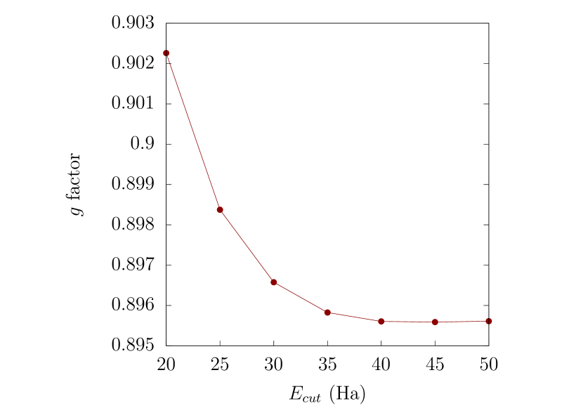
Figure 1: Convergence of the $g$ factor of H₂ (with $d_{\text{exp}}=1.4$ bohr) with respect to the plane-wave cutoff. Calculations are performed using a single $\mathbf{k}$ point ($\Gamma$) with a box size of $20^{3}$ bohr³.

Since the H atom is well described by a local pseudopotential, we can use the H₂ molecule to benchmark the performance of the two alternative formulations of $\partial m_{a}/\partial\omega_{b}$, i.e. Eq. (26) [which reduces to Eq. (56) in this case] and Eq. (28). In Fig. 2(a) we the plot the calculated $g$ factor for H₂ versus inverse cell size by using either method. As we anticipated in Sec. II.3, we find that Eq. (28) is quite challenging to converge, while the corresponding results of Eq. (56) display an optimally fast convergence. To understand the origin of such a behavior, we show in Fig. 2(b) a decomposition of Eq. (28) into the two contributions on the rhs. This analysis clarifies that the convergence of is limited by the quadrupole term [i.e., the second term in Eq. (28)], while the magnetic susceptibility of the molecule is already converged at a relatively small box size. If we extrapolate this term to the limit of an infinitely large cell parameter ($1/a\rightarrow 0$, purple dashed curve), then we see that our $g$ factor indeed converges to the value we obtain using the methodology of Sec. III.2 [purple cross on Fig. 2(a)]. The agreement for large cell sizes provides an independent confirmation of the accuracy of our approach, though the methodology of Sec. III.2 is clearly superior from a computational perspective.

As we anticipated, a further issue with Eq. (28) consists in the fact that it may yield qualitatively incorrect results when nonlocal pseudopotentials are used, i.e., in the vast majority of first-principles simulations that are being performed nowadays. An obvious example is that of a neutral (and isolated) closed-shell atom, where the rotationally induced magnetization must vanish exactly. This requirement is trivially fulfilled by our Eq. (26): both dynamical charges and dynamical magnetic moments identically vanish in this system due to charge neutrality and inversion symmetry. In the context of Eq. (28) one would expect a vanishing result, too: Langevin’s theory of diamagnetism expresses the susceptibility as the quadrupolar moment of the spherical atomic charge, which should cancel out exactly with the second term on the rhs. In presence of nonlocal pseudopotentials, however, Langevin’s result no longer holds, and Eq. (28) yields a nonzero value for all noble gas atoms except He. (The latter, just like H, is well described by a local pseudopotential.) We regard this as a serious concern in this context, and we therefore caution against a straightforward application of Eq. (28) to the calculation of rotational $g$ factors.

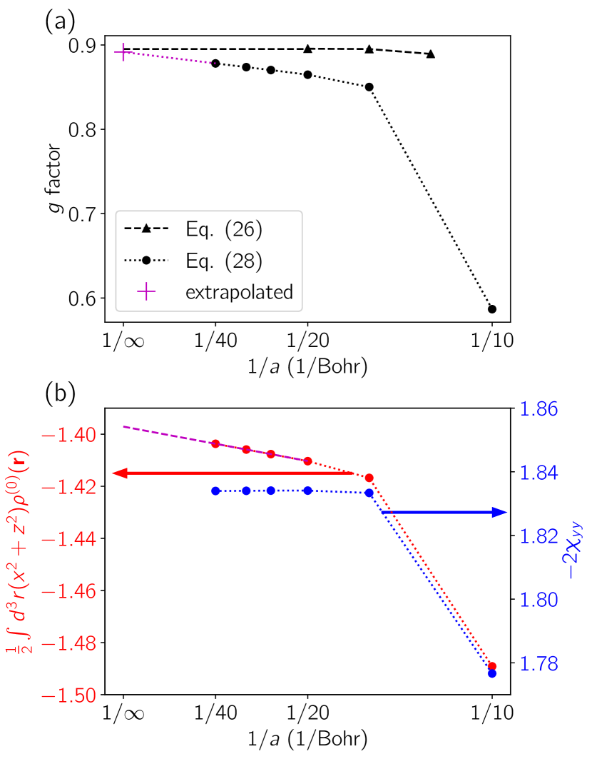
Figure 2: (a) Calculation of rotational $g$ factor of H₂ (with $d_{\text{exp}}$=1.4 bohr) using the expression for $\partial m_{a}/\partial\omega_{b}$ from Eq. (28) (dots) and from Eq. (26) (triangles) versus inverse of the simulation cell size side length. (b) Convergence of terms in Eq. (28) versus inverse of the simulation cell size. Purple dashed line in (b) is the extrapolated value for the quadrupole term; the purple cross in (a) is the $g$ factor calculated with the extrapolated quadrupole term.

In addition to the aforementioned elemental diatomic molecules, we consider several other examples: HF, HNC, and FCCH (still linear, but with a finite dipole moment), nonlinear molecules such as NH₃, H₂O, and CH₄, and the aromatic compounds C₅H₅F and C₆H₅F. At difference with H₂ and related structures, in all these cases Eq. (24) contains a nonzero contribution from the Born effective charges; therefore, these additional examples provide us with the opportunity to test the full formula, Eq. (26) [in combination with Eq. (24)], rather than its simplified version, Eq. (56). The molecular geometries and rotational axes used in this work are discussed in Appendix C.

Table 1: Calculated rotational $g$ factors for selected simple molecules compared with the relevant literature data. “HF/DFT” and “MP/CCD” stand for computational results at various level of theory (Hartree-Fock / Density Functional Theory, and Møller-Plesset perturbation theory / Coupled-Cluster with Double excitations); “Exp.” refers to experimental measurements.

	Rotational $g$ factor
	This work	HF/DFT	MP/CDD	Exp.
H2	0.8901	$0.9103$	0.8899	$0.8829$
		0.8755
N2	$-0.2699$	$-0.2872$	$-0.2653$	$-0.2593$
F2	$-0.1003$	$-0.0900$	$-0.1136$	$-0.1208$
HF	0.7603	0.7624	0.7488	0.7392
HNC	$-0.1004$	$-0.0996$	$-0.0968$
FCCH	$-0.0065$			$-0.0077$
H2O	0.6699	0.6640	0.6507	0.6450
NH3	0.5289	0.5061	0.5044
CH4	0.3629	0.3019	0.3190	$0.3133$
		0.2985
C5H5N	0.0411			0.0428
C6H5F	0.0276			0.0266

In Table 1 we compare our results for the rotational $g$ factors to experimental measurements from Refs.  Flygare and Benson, 1971 and  Flygare, 1974. In addition, we report the results of previous calculations using Hartree-Fock (HF) and post Hartree-Fock methodsCybulski and Bishop (1997), as well as DFT calculations using the Berry-phase method Ceresoli and Tosatti (2002, ). Since the inclusion of electron-electron correlations, either at at the level of Møller-Plesset (MP) perturbation theory or coupled cluster with double excitations (CCD), seems to improve the agreement with experiment in many cases, Cybulski and Bishop (1997) we include those data as well for comparison. We see that our DFPT based method compares well even with the best theoretical values obtained via more computationally demanding methods. Our results in Table 1 are also in excellent agreement with experiment, where available. CH₄ appears to be the only exception, though the reason for the larger discrepancy is not clear.

IV.2 Soft-mode frequency splitting of cubic SrTiO₃

Table 2: $g$ factor of the soft polar TO mode at the zone center in cubic SrTiO₃. Units are in $10^{-4}$ atomic units.

	$g$	$g^{\text{pc}}$	$g^{\text{di}}$
SrTiO3	$-1.2083$	$0.6679$	$-1.8763$

We now turn to the splitting of the soft polar TO mode at the zone center in cubic SrTiO₃. As we did in the case of the rotational $g$ factors in Sec. IV.1, we can test the accuracy of our generalized Lorentz forces by comparing the implementation described in Sec. III.2 with the alternative approach of Sec. III.1. In Table 5 of Appendix D we present the components of $(D^{\text{di,}\gamma})_{\kappa\alpha,\kappa^{\prime}\beta}$ elements [see Eq. (36)] for cubic SrTiO₃ using both methods; we see quite good agreement, giving us confidence that $g^{\text{di}}$ is accurately calculated.

The results for the $g$ factors are shown in Table 2. Following Eq. (45), we separate the two different contributions coming from the $\mathbf{J}^{(0)}$ ($g^{\text{pc}}$) and $\mathbf{J}^{(1)}$ ($g^{\text{di}}$) terms. As mentioned earlier, some worksJuraschek et al. (2017); Juraschek and Spaldin (2019) have only accounted for the terms depending on the Born effective charges within a point-charge approximation, roughly corresponding to our calculated $g^{\text{pc}}$. It is immediately clear from Table 2 that such an approximation is inappropriate: the remainder ($g^{\text{di}}$) has opposite sign and is almost three times larger (in absolute value) than the contribution coming from $g^{\text{pc}}$; as a result, the total $g$ factor disagrees with $g^{\text{pc}}$ both in magnitude and sign. This indicates that an accurate computation of the $\mathbf{J}^{(1)}$ tensor is crucial in this particular case and that these terms should not be neglected.

For a more quantitative comparison, note that Ref.  Ceresoli, 2002 and Ref.  Juraschek et al., 2017 computed $g^{\text{pc}}$ for tetragonal SrTiO₃, obtaining values of $g^{\text{pc}}=5.76\cdot 10^{-5}\text{cm}^{-1}/\text{T}$ and $g^{\text{pc}}=4.78\cdot 10^{-5}\text{cm}^{-1}/\text{T}$, respectively. In those units, our result for cubic SrTiO₃ is $g^{\text{pc}}=6.23\cdot 10^{-5}\text{cm}^{-1}/\text{T}$. The agreement is rather good, especially considering that: (i) we are considering the full tensorial form of the Born effective charge tensor and (ii) our analysis is carried out in the cubic, and not tetragonal, phase of SrTiO₃. Note that Ref.  Ceresoli, 2002 also reports a result for the total $g$-factor, $g=-7.95\cdot 10^{-5}\text{cm}^{-1}/\text{T}$, which again compares well to our calculated value of $g=-11.28\cdot 10^{-5}\text{cm}^{-1}/\text{T}$.

To gain some insight on the physics, we perform a further decomposition of $g^{\text{pc}}$ and $g^{\text{di}}$ into the individual contributions of each atomic sublattice. In the case of $g^{\text{pc}}$, such a decomposition is straightforward, as this term mediates an on-site coupling between the displacement of each atom and its own velocity. [This can be appreciated by observing that the corresponding contribution to the generalized Lorentz force, Eq. (34), contains a $\delta_{\kappa\kappa^{\prime}}$ prefactor.] The case of $g^{\text{di}}$ is less obvious: the nondiagonal (on the atomic index) nature of $\Phi^{\rm di}$ implies that the velocity of a given atom can produce forces not only onto itself, but also on its neighbors. Thus, prior to attempting a decomposition of $g^{\text{di}}$, we first isolate the basis-diagonal $\kappa=\kappa^{\prime}$ terms in $\Phi^{\rm di}$, and use them to define an on-site contributions to $g^{\text{di}}$ (indicated as $g^{\text{di}}_{\kappa=\kappa^{\prime}}$ henceforth). Apart from enabling the aforementioned decomposition, this analysis also gives a flavor of the overall importance of the off-site contributions to $g^{\text{di}}$.

Table 3: Contribution of each atom to $g^{\text{pc}}$ and $g^{\text{di}}_{\kappa=\kappa^{\prime}}$, which are defined as the on-site ($\kappa=\kappa^{\prime}$) contributions to $g^{\text{di}}$. Units are in $10^{-4}$ atomic units.

	Sr	Ti	O1	O2	O3	total
$g^{\text{pc}}$	-0.0197	-0.1082	0.2985	0.2985	0.1987	0.6679
$g^{\text{di}}_{\kappa=\kappa^{\prime}}$	-0.0118	-0.1246	-0.6429	-0.6429	-0.0062	-1.4284

The results are summarized in Table 3. Regarding $g^{\text{pc}}$, we find that the contribution of the oxygen atoms largely dominates over the rest, consistent with the conclusions of Ref.  Ceresoli, 2002. Due to their smaller mass, oxygens evolve along larger orbits, which amplifies their contribution to the magnetic moment. Regarding $g^{\text{di}}$, we find that the on-site terms represent more than the $75\%$ of the total $g^{\text{di}}$ factor, which indicates that intersite couplings have a relatively minor importance. At the level of $g^{\text{di}}_{\kappa=\kappa^{\prime}}$, we find that the contribution of the equatorial oxygens is by far the largest, and primarily responsible for reversing the sign of the overall $g$ factor.

Finally, we use the above results to calculate the frequency splitting of the TO modes. Considering a magnetic field of $B=100$ T we obtain $gB\sim 0.01\text{ cm}^{-1}$, of the same order as predicted in Ref.  Juraschek and Spaldin, 2019. This is a very small value that appears challenging to resolve even for the most powerful experimental techniques available nowadays. Our hope is that the computational tools developed here allow for a more efficient screening of candidate materials where this effect may be measurable.

V Conclusions

We have developed a complete theoretical approach for calculating orbital magnetization from rotations and pseudorotations (circularly polarized optical phonons) within the context of first-principles theory. The approach is based on density-functional perturbation theory calculations of the polarization induced by an atomic displacement (i.e., Born effective charges), and its first real-space moment. We have demonstrated an implementation to calculate the latter quantity via generalization of the existing long-wave approach to dynamical quadrupoles; thus, we have established a connection between spatial dispersion phenomena and orbital magnetism, and demonstrated its accuracy via comparison with finite-difference calculations. Our methodology allows for efficient and optimally accurate computation, and works equally well for molecules and solids. We have used this approach to determine rotational $g$ factors of some simple molecules, and demonstrated excellent agreement with experimental results where available. Finally, we have developed a strategy to calculate the generalized Lorentz force on atoms in presence of a magnetic field, and utilized it to study the splitting of the soft optical phonons in cubic SrTiO₃. In the latter system, we demonstrated that contributions to phonon $g$ factor from the first moment of the induced polarization, which had been neglected in some previous approaches, dominate the response.

In spite of this correction, the overall $g$ factor remains of the same order of magnitude as the values quoted in Refs.  Juraschek and Spaldin, 2019; Ceresoli, 2002. Therefore, our theory as it stands appears unlikely to explain the large phonon Hall Li et al. (2020) effects reported experimentally. To move forward in this direction, we suspect that it may be necessary to take into account the quantum paralectric nature of SrTiO₃ at low temperatures, e.g., by going beyond the Ehrenfest Lagrangian of Eq. (1). We regard this as an exciting avenue for further study.

Appendix A Translational symmetry of the geometric magnetization

To see how a change in the assumed center of rotation (and, simultaneously, in the gauge origin) affects the result, consider

$$\begin{split}\frac{\partial m_{a}({\bf R})}{\partial\omega_{b}}=&\sum_{\kappa,j,\beta}\epsilon^{bj\beta}(\tau_{\kappa j}-R_{j})\times\\ &\left[\mathcal{M}_{a,\kappa\beta}+\frac{1}{2}\sum_{i,\alpha}\epsilon^{ai\alpha}(\tau_{\kappa i}-R_{i})J^{(0)}_{\alpha,\kappa\beta}\right]\\ =&-\sum_{\kappa,j,\beta}\epsilon^{bj\beta}R_{j}\left[\mathcal{M}_{a,\kappa\beta}+\frac{1}{2}\sum_{i,\alpha}\epsilon^{ai\alpha}\tau_{\kappa i}J^{(0)}_{\alpha,\kappa\beta}\right]\\ &-\frac{1}{2}\sum_{\kappa,j,\beta,i,\alpha}\epsilon^{bj\beta}\epsilon^{ai\alpha}\tau_{\kappa j}R_{i}J^{(0)}_{\alpha,\kappa\beta}+\frac{\partial m_{a}({\bf 0})}{\partial\omega_{b}}\\ =&-\frac{1}{2}\sum_{\kappa,j,i,\alpha}\epsilon^{bj\alpha}\epsilon^{ai\alpha}R_{j}\mathcal{D}_{i}\\ &-\frac{1}{2}\sum_{\kappa,j,\beta,i,\alpha}\epsilon^{bj\beta}\epsilon^{ai\alpha}\tau_{\kappa j}R_{i}J^{(0)}_{\alpha,\kappa\beta}+\frac{\partial m_{a}({\bf 0})}{\partial\omega_{b}}.\end{split}$$ (57)

[In the last step we have used the sum rule Eq. (19).] It is useful now to observe the following property of the Levi-Civita symbol,

$$\sum_{i,j,\alpha}\epsilon^{bj\alpha}\epsilon^{ai\alpha}=\delta_{ab}\delta_{ij}-\delta_{bi}\delta_{aj}.$$ (58)

This leads to

$$\begin{split}-\frac{1}{2}\sum_{\kappa,j,i,\alpha}\epsilon^{bj\alpha}\epsilon^{ai\alpha}R_{j}\mathcal{D}_{i}=&-\frac{1}{2}(\delta_{ab}{\bf R}\cdot\bm{\mathcal{D}}-R_{a}\mathcal{D}_{b}).\end{split}$$ (59)

In the second line we can write

$$\begin{split}-\sum_{\kappa}\tau_{\kappa j}J^{(0)}_{\alpha,\kappa\beta}=&\sum_{\kappa}J^{(1,j)}_{\alpha,\kappa\beta}-\mathcal{D}_{j}.\end{split}$$ (60)

The second term yields the same as above, with the $ab$ indices switched; the first term can be written in terms of $J^{(1)}$. The final result, after collecting all the contributions is

$$\begin{split}\frac{\partial m_{a}({\bf R})}{\partial\omega_{b}}&-\frac{\partial m_{a}({\bf 0})}{\partial\omega_{b}}=\\ =&-\frac{1}{2}(\delta_{ab}{\bf R}\cdot\bm{\mathcal{D}}-R_{a}\mathcal{D}_{b}-R_{b}\mathcal{D}_{a})\\ &+\frac{1}{2}\sum_{j,\beta,i,\alpha}\epsilon^{bj\beta}\epsilon^{ai\alpha}R_{i}\sum_{\kappa}J^{(1,j)}_{\alpha,\kappa\beta}.\end{split}$$ (61)

The second term on the rhs vanishes: the sublattice sum of the $J^{(1,j)}_{\alpha,\kappa\beta}$ tensor coincides with the proper piezoelectric tensor times a trivial volume factor, and is therefore symmetric with respect to $\beta j$. (An antisymmetric contribution would describe a steady macroscopic current that is generated by a rotating body in its comoving reference frame, and must vanish on general physical grounds, see Sec. III.D.2 of Ref.  Stengel and Vanderbilt, 2018.) The remainder leads to Eq. (27).

Appendix B Dipolar sum rule for bounded systems

Statement of the problem. We will prove the following sum rule, valid for an isolated molecule in open electrostatic boundary conditions,

$$\sum_{\kappa}\left(J_{\alpha,\kappa\beta}^{(1,\gamma)}+\tau_{\kappa\gamma}Z^{*}_{\alpha,\kappa\beta}\right)=\delta_{\alpha\beta}\mathcal{D}_{\gamma},$$ (62)

where $\bm{\mathcal{D}}$ is the static dipole moment of the molecule,

$$\mathcal{D}_{\gamma}=\int d^{3}rr_{\gamma}\rho^{(0)}({\bf r}).$$ (63)

In absence of nonlocal pseudopotentials the proof is straightforward: it suffices to observe that $Z^{*}_{\alpha,\kappa\beta}=J^{(0)}_{\alpha,\kappa\beta}$, and then use the definition of the $J^{(n)}_{\alpha,\kappa\beta}$ moments provided in the main text together with the following relation (translational invariance) for the microscopic polarization response,

$$\sum_{\kappa}\mathcal{P}_{\alpha,\kappa\beta}({\bf r})=\delta_{\alpha\beta}\rho^{(0)}({\bf r}).$$ (64)

If nonlocal pseudopotentials are present, Eq. (64) breaks down; however, we will show that Eq. (62) is exact even in that case.

Proof. To prove Eq. (62) without passing through Eq. (64), we will use another (exact) sum rule, relating the $J_{\alpha,\kappa\beta}^{(1,\gamma)}$ moments to the clamped-ion piezoelectric tensor,

$$-\frac{1}{\Omega}\sum_{\kappa}J_{\alpha,\kappa\beta}^{(1,\gamma)}=\bar{e}_{\alpha,\beta\gamma}.$$ (65)

To apply this rule, we need first of all to place the isolated molecule in a large box of volume $\Omega$, and work in periodic boundary conditions. Then, Eq. (65) describes the proper piezoelectric response of the resulting crystal lattice to an infinitesimal strain. [To avoid complications due to long-range interactions between repeated images, we will assume that the Coulomb kernel is cut off at the boundary of the box, and that all objects entering Eq. (62) are consistently calculated in such conditions.]

Since the images of the molecule are isolated in space, the macroscopic polarization of the crystal is exactly given by the Clausius-Mossotti formula as the static dipole moment divided by the volume,

$${\bf P}=\frac{\bm{\mathcal{D}}}{\Omega}.$$ (66)

$\bar{e}_{\alpha,\beta\gamma}$, however, is not defined as a straightforward strain derivative of ${\bf P}$ (that would be the so-called improper piezoelectric tensor). To arrive at $\bar{e}_{\alpha,\beta\gamma}$ we first need to introduce the direct lattice vectors ${\bf a}_{i}$ and their duals ${\bf b}_{i}$ in such a way that ${\bf a}_{i}\cdot{\bf b}_{j}=\delta_{ij}$. Then, the reduced polarization is defined in units of charge as the flux of ${\bf P}$ through a facet of the crystal cell,

$$p_{i}=\Omega{\bf b}_{i}\cdot{\bf P}={\bf b}_{i}\cdot\bm{\mathcal{D}}.$$ (67)

Finally, the proper piezoelectric tensor is defined as

$$\bar{e}_{\alpha,\beta\gamma}=\frac{1}{\Omega}\sum_{i}a_{\alpha i}\frac{\partial p_{i}}{\partial\eta_{\beta\gamma}},$$ (68)

where $\boldsymbol{\eta}$ is the Cauchy infinitesimal strain tensor. This leads to the following formula, without factors of volume,

$$\sum_{\kappa}J_{\alpha,\kappa\beta}^{(1,\gamma)}=-\sum_{i}({\bf a_{i}})_{\alpha}\frac{\partial({\bf b}_{i}\cdot\bm{\mathcal{D}})}{\partial\eta_{\beta\gamma}}.$$ (69)

In order to calculate the derivative of the scalar product, note that an infinitesimal strain corresponds to the following linear transformation of the atomic coordinates and direct lattice vectors,

$$\bm{\tau}^{\prime}_{\kappa}= ({\bf I}+\bm{\eta})\bm{\tau}_{\kappa},$$ (70a)

$${\bf a}^{\prime}_{i}= ({\bf I}+\bm{\eta}){\bf a}_{i}.$$ (70b)

The first relation yields

$$\frac{\partial\tau_{\kappa\sigma}}{\partial\eta_{\beta\gamma}}=\delta_{\beta\sigma}\tau_{\kappa\gamma},$$ (71)

and immediately (by using the definition of the Born charge tensor),

$$\frac{\partial\mathcal{D}_{\alpha}}{\partial\eta_{\beta\gamma}}=\sum_{\kappa\sigma}\frac{\partial\mathcal{D}_{\alpha}}{\partial\tau_{\kappa\sigma}}\frac{\partial\tau_{\kappa\sigma}}{\partial\eta_{\beta\gamma}}=\sum_{\kappa}Z^{*}_{\alpha,\kappa\beta}\tau_{\kappa\gamma}.$$ (72)

The second relation is used to determine the transformation law for the duals. The reciprocal-space vectors need to preserve the orthonormality condition to linear order in the strain, which leads to the following result,

$${\bf b}^{\prime}_{i}\simeq({\bf I}-\bm{\eta}^{T}){\bf b}_{i}.$$ (73)

From this, we deduce

$$\frac{\partial({\bf b}_{i})_{\xi}}{\partial\eta_{\beta\gamma}}=-\delta_{\gamma\xi}({\bf b}_{i})_{\beta}.$$ (74)

By using the orthonormality rule $\sum_{i}({\bf a_{i}})_{\alpha}({\bf b}_{i})_{\beta}=\delta_{\alpha\beta}$, we eventually arrive at

$$\sum_{\kappa}J_{\alpha,\kappa\beta}^{(1,\gamma)}=\mathcal{D}_{\gamma}-\sum_{\kappa}Z^{*}_{\alpha,\kappa\beta}\tau_{\kappa\gamma},$$ (75)

thereby concluding our proof.

General consequences. The above results allow us to further specify the validity of Eq. (64) in the case of an isolated molecule. While the microscopic formula breaks down in presence of nonlocal pseudopotentials, one can expand both sides into Cartesian multipoles and ask at what order the equality no longer holds. At order zero the equality clearly holds,

$$\sum_{\kappa}\int d^{3}r\mathcal{P}_{\alpha,\kappa\beta}({\bf r})=\delta_{\alpha\beta}\int d^{3}r\rho^{(0)}({\bf r}),$$ (76)

since macroscopic currents are well described; in the case of a neutral molecule Eq. (76) reduces to the acoustic sum rule on the Born charge tensor components. In this Appendix, we have provided a formal proof that Eq. (64) works equally well at first order,

$$\sum_{\kappa}\int d^{3}r\,r_{\gamma}\mathcal{P}_{\alpha,\kappa\beta}({\bf r})=\delta_{\alpha\beta}\int d^{3}r\,r_{\gamma}\rho^{(0)}({\bf r}).$$ (77)

On the other hand, we already know from earlier works that the second order doesn’t work if nonlocal potentials are used in the calculation,

$$\sum_{\kappa}\int d^{3}r\,r_{\gamma}r_{\lambda}\mathcal{P}_{\alpha,\kappa\beta}({\bf r})\neq\delta_{\alpha\beta}\int d^{3}r\,r_{\gamma}r_{\lambda}\rho^{(0)}({\bf r}).$$ (78)

This breakdown of translational invariance at the quadrupolar level explains why Eq. (26) and Eq. (28) disagree in presence of nonlocal potentials.

Appendix C Structure of molecules used in this work

Here we show the molecular structures used in this work. For the aromatic compounds, we also display a cartoon of the molecules in Figure 3, labeling each atom with a number. This figure, in combination with Table 4, enables to construct the C₅H₅N and C₅H₅F molecules.

In order to calculate the $g$ factor, the rotation axis is taken to be perpendicular to the molecular axis in linear molecules (H₂, N₂, F₂, HF, HNC, and FCCH), perpendicular to the molecular plane for C₅H₅N, C₆H₅F and H₂O, along one of the bonds in CH₄ and perpendicular to the plane formed by the H atoms in NH₃; the field is taken to be parallel to the rotation axis.

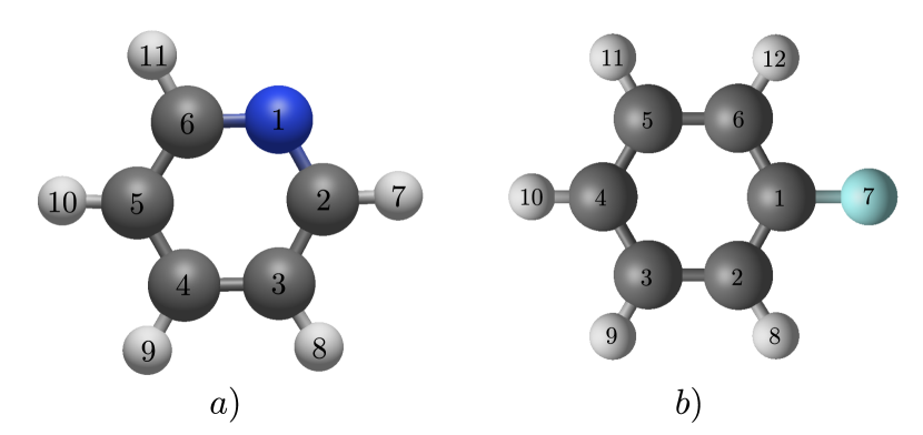
Figure 3: Cartoon illustrating the relaxed geometries used in this work for a) C₅H₅N (the N atom is in blue) and b) C₆H₅F (F atom is in light blue).

Table 4: Molecular geometries for selected simple molecules after relaxation. Distances are in bohr.

	Relaxed geometry
H2	$d=1.446$
N2	$d=2.066$
F2	$d=2.622$
HF	$d=1.760$
HNC	$d_{\text{HN}}=1.908$
	$d_{\text{NC}}=2.202$
FCCH	$d_{\text{FC}}=2.396$
	$d_{\text{CC}}=2.260$
	$d_{\text{CH}}=2.022$
H2O	$d_{\text{HO}}=1.835$
	$\angle\text{HOH}=104.8^{\circ}$
NH3	$d_{\text{NH}}=1.930$
	$\angle\text{HNH}=107.3^{\circ}$
CH4	$d_{\text{CH}}=2.070$
C5H5N	$d_{1,2}=2.509$, $d_{2,3}=2.615$
	$d_{3,4}=2.611$, $d_{2,7}=2.071$
	$d_{3,8}=2.063$, $d_{4,9}=2.064$
	$\angle 6,1,2=117.54^{\circ}$, $\angle 1,2,3=123.42^{\circ}$
	$\angle 2,3,4=118.52^{\circ}$, $\angle 3,4,5=118.58^{\circ}$
C5H5F	$d_{1,2}=2.603$, $d_{2,3}=2.614$
	$d_{3,4}=2.616$, $d_{1,7}=2.534$
	$d_{2,8}=2.062$, $d_{3,9}=2.063$
	$d_{4,10}=2.062$, $\angle 6,1,2=122.43^{\circ}$
	$\angle 1,2,3=118.40^{\circ}$, $\angle 2,3,4=120.45^{\circ}$
	$\angle 3,4,5=119.86^{\circ}$

Appendix D Comparison between DFPT and finite $q$ calculations for cubic SrTiO₃

Here we present a comparison between the “DFPT” implementation described in Sec. III.2, and the “finite $q$” implementation described in Sec. III.1 for the generalized Lorentz force in cubic SrTiO₃. Specifically, we compare the $(D^{\text{di,}z})_{\kappa\alpha,\kappa^{\prime}\beta}$ elements, see Eq. (36). All of the independent elements for both methods are presented in Table 5. Note that our labeling convention for the oxygen is, in reduced coordinates: $\text{O}1=(0,1/2,1/2)$, $\text{O}2=(1/2,0,1/2)$, $\text{O}3=(1/2,1/2,0)$. The additional $(\kappa\alpha,\kappa^{\prime}\beta)$ can be determined from the following symmetry requirements on the tensor in cubic SrTiO₃. For $\kappa$ and $\kappa^{\prime}$ either (or both) Ti, Sr, or O3, $x\leftrightarrow y$ results in the same magnitude coefficient, with a change of sign. For terms involving O1 and/or O2, exchanging $x\leftrightarrow y$ as well as $\text{O}1\leftrightarrow\text{O}2$ also results in a different sign, but same magnitude coefficient. Overall, we see quite good agreement, to the second or third decimal places, between the very distinct implementations; this confirms the accuracy of our methodology.

Table 5: $(D^{\text{di,}z})_{\kappa\alpha,\kappa^{\prime}\beta}$ elements [see Eq. (36)] for cubic SrTiO₃ calculated with the “DFPT” implementation described in Sec. III.2, and the “finite $q$” implementation described in Sec. III.1.

$(\kappa\alpha,\kappa^{\prime}\beta)$	DFPT	Finite $q$
(Sr $x$, Sr $y$)	$1.5320$	$1.5317$
(Sr $x$, Ti $y$)	$2.4483$	$2.4526$
(Sr $x$, O1 $y$)	$-0.4487$	$-0.4489$
(Sr $x$, O2 $y$)	$-2.3829$	$-2.3874$
(Sr $x$, O3 $y$)	$-1.1537$	$-1.1542$
(Ti $x$, Ti $y$)	$8.4125$	$8.4037$
(Ti $x$, O1 $y$)	$-9.6112$	$-9.6131$
(Ti $x$, O2 $y$)	$-2.4061$	$-2.3937$
(Ti $x$, O3 $y$)	$3.7315$	$3.7336$
(O1 $x$, O2 $y$)	$-6.3272$	$-6.3416$
(O2 $x$, O1 $y$)	$3.9400$	$3.9416$
(O2 $x$, O2 $y$)	$8.3977$	$8.3987$
(O3 $x$, O1 $y$)	$-0.3842$	$-0.3845$
(O3 $x$, O2 $y$)	$-2.0026$	$-2.0041$
(O3 $x$, O3 $y$)	$0.0642$	$0.0653$

References

- Ceresoli and Tosatti (2002) D. Ceresoli and E. Tosatti, Phys. Rev. Lett. 89, 116402 (2002).
- Trifunovic, Ono, and Watanabe (2019) L. Trifunovic, S. Ono, and H. Watanabe, Phys. Rev. B 100, 054408 (2019).
- Ceresoli, Marchetti, and Tosatti (2007) D. Ceresoli, R. Marchetti, and E. Tosatti, Phys. Rev. B 75, 161101 (2007).
- Qin, Zhou, and Shi (2012) T. Qin, J. Zhou, and J. Shi, Phys. Rev. B 86, 104305 (2012).
- Juraschek and Spaldin (2019) D. M. Juraschek and N. A. Spaldin, Phys. Rev. Mater. 3, 064405 (2019).
- Juraschek et al. (2017) D. M. Juraschek, M. Fechner, A. V. Balatsky, and N. A. Spaldin, Phys. Rev. Mater. 1, 014401 (2017).
- Sun, Gao, and Wang (2021) K. Sun, Z. Gao, and J.-S. Wang, Phys. Rev. B 103, 214301 (2021).
- Zhang et al. (2010) L. Zhang, J. Ren, J.-S. Wang, and B. Li, Phys. Rev. Lett. 105, 225901 (2010).
- Culpitt et al. (2021) T. Culpitt, L. D. Peters, E. I. Tellgren, and T. Helgaker, J. Chem. Phys. 155, 024104 (2021).
- Peters et al. (2021) L. D. Peters, T. Culpitt, L. Monzel, E. I. Tellgren, and T. Helgaker, J. Chem. Phys. 155, 024105 (2021).
- Cybulski and Bishop (1997) S. M. Cybulski and D. M. Bishop, J. Chem. Phys. 106, 4082 (1997).
- Ceresoli (2002) D. Ceresoli, Ph.D. thesis (2002).
- Ceresoli et al. (2006) D. Ceresoli, T. Thonhauser, D. Vanderbilt, and R. Resta, Phys. Rev. B 74, 024408 (2006).
- Shi et al. (2007) J. Shi, G. Vignale, D. Xiao, and Q. Niu, Phys. Rev. Lett. 99, 197202 (2007).
- Resta (2010) R. Resta, J. Phys. Condens. Matter 22, 123201 (2010).
- Cai and Galli (2004) W. Cai and G. Galli, Phys. Rev. Lett. 92, 186402 (2004).
- Lee, Cai, and Galli (2007) E. Lee, W. Cai, and G. A. Galli, J. Comput. Phys. 226, 1310 (2007).
- Williams-Young et al. (2019) D. B. Williams-Young, A. Petrone, S. Sun, T. F. Stetina, P. Lestrange, C. E. Hoyer, D. R. Nascimento, L. Koulias, A. Wildman, J. Kasper, J. J. Goings, F. Ding, A. E. DePrince III, E. F. Valeev, and X. Li, Wiley Interdiscip. Rev. Comput. Mol. Sci. , e1436 (2019).
- Balasubramani et al. (2020) S. G. Balasubramani, G. P. Chen, S. Coriani, M. Diedenhofen, M. S. Frank, Y. J. Franzke, F. Furche, R. Grotjahn, M. E. Harding, C. Hättig, et al., J. Chem. Phys. 152, 184107 (2020).
- Stengel (2013) M. Stengel, Phys. Rev. B 88, 174106 (2013).
- Gonze and Lee (1997) X. Gonze and C. Lee, Phys. Rev. B 55, 10355 (1997).
- Giannozzi et al. (1991) P. Giannozzi, S. de Gironcoli, P. Pavone, and S. Baroni, Phys. Rev. B 43, 7231 (1991).
- Ghosez, Michenaud, and Gonze (1998) P. Ghosez, J.-P. Michenaud, and X. Gonze, Phys. Rev. B 58, 6224 (1998).
- Dreyer, Stengel, and Vanderbilt (2018) C. E. Dreyer, M. Stengel, and D. Vanderbilt, Phys. Rev. B 98, 075153 (2018).
- Royo and Stengel (2019) M. Royo and M. Stengel, Phys. Rev. X 9, 021050 (2019).
- Romero et al. (2020) A. H. Romero et al., J. Chem. Phys. 152, 124102 (2020).
- Gonze et al. (2009) X. Gonze, B. Amadon, P.-M. Anglade, J.-M. Beuken, F. Bottin, P. Boulanger, F. Bruneval, D. Caliste, R. Caracas, M. Côté, et al., Comput. Phys. Commun. 180, 2582 (2009).
- Gonze et al. (2020) X. Gonze, B. Amadon, G. Antonius, F. Arnardi, L. Baguet, J.-M. Beuken, J. Bieder, F. Bottin, J. Bouchet, E. Bousquet, et al., Comput. Phys. Commun. 248, 107042 (2020).
- Stengel and Vanderbilt (2018) M. Stengel and D. Vanderbilt, Phys. Rev. B 98, 125133 (2018).
- Li et al. (2020) X. Li, B. Fauqué, Z. Zhu, and K. Behnia, Phys. Rev. Lett. 124, 105901 (2020).
- Mead and Truhlar (1979) C. Mead and D. Truhlar, J. Chem. Phys. 70, 2284 (1979).
- Martin (1972) R. M. Martin, Phys. Rev. B 5, 1607 (1972).
- Brown et al. (2000) J. M. Brown et al., Mol. Phys. 98, 1597 (2000).
- Cybulski and Bishop (1994) S. M. Cybulski and D. M. Bishop, J. Chem. Phys. 100, 2019 (1994).
- Roman et al. (2006) E. Roman, J. R. Yates, M. Veithen, D. Vanderbilt, and I. Souza, Phys. Rev. B 74, 245204 (2006).
- Cowley (1964) R. A. Cowley, Phys. Rev. 134, A981 (1964).
- Baroni et al. (2001) S. Baroni, S. de Gironcoli, A. Dal Corso, and P. Giannozzi, Rev. Mod. Phys. 73, 515 (2001).
- Essin et al. (2010) A. M. Essin, A. M. Turner, J. E. Moore, and D. Vanderbilt, Phys. Rev. B 81, 205104 (2010).
- Gonze (1997) X. Gonze, Phys. Rev. B 55, 10337 (1997).
- Perdew and Wang (1992) J. P. Perdew and Y. Wang, Phys. Rev. B 45, 13244 (1992).
- Hamann (2013) D. R. Hamann, Phys. Rev. B 88, 085117 (2013).
- Flygare and Benson (1971) W. Flygare and R. Benson, Mol. Phys. 20, 225 (1971).
- Flygare (1974) W. Flygare, Chem. Rev. 74, 653 (1974).
- (44) D. Ceresoli and E. Tosatti, Private Communication.