Resolved Gaia Triples

Abstract

A sample of 392 low-mass hierarchical triple stellar systems within 100 pc resolved by Gaia as distinct sources is defined. Owing to the uniform selection, the sample is ideally suited to study unbiased statistics of wide triples. The median projected separations in their inner and outer pairs are 151 and 2569 au, respectively, the median separation ratio is close to 15. Some triples appear in non-hierarchical configurations, and many are just above the dynamical stability limit. Internal motions in these systems are known with sufficient accuracy to determine the orbital motion sense of the outer and inner pairs and to reconstruct the eccentricity distributions. The mean inner and outer eccentricities are 0.66$\pm$0.02 and 0.54$\pm$0.02, respectively; the less eccentric outer orbits are explained by dynamical stability. The motion sense of the inner and outer pairs is almost uncorrelated, implying a mean mutual inclination of $83\fdg 1\pm 4\fdg 5$. The median mass of the most massive component is 0.71 $M_{\odot}$ , the median system mass is 1.53 $M_{\odot}$ . In a 0.69 fraction of the sample the primary belongs to the inner binary, while in the remaining systems it is the tertiary. A 0.21 fraction of the inner subsystems are twins with mass ratios $>$0.95. The median outer mass ratio is 0.41; it decreases mildly with increasing outer separation. Presumably, these wide hierarchies were formed by collapse and fragmentation of isolated cores in low-density environments and represent a small fraction of initial systems that avoided dynamical decay. Wide pre-main sequence multiples in Taurus could be their progenitors.

1 Introduction

Binary stars and high-order hierarchical systems are typical products of star formation. Parameters of stellar systems (periods, mass ratios, eccentricies) provide valuable insights into star formation, environment, and early evolution, and serve as benchmarks to compare with simulations (e.g. Bate, 2014; Lomax et al., 2015). This fact has been widely recognized regarding binary stars, motivating their numerous statistical studies (Duchêne & Kraus, 2013; Moe & Di Stefano, 2017, and references therein). Stellar hierarchies containing three or more stars are even more interesting from this point of view, but they are studied much less. The reason is a lack of unbiased samples of hierarchies because their discovery is difficult and usually requires combination of various techniques such as high-resolution imaging and spectroscopy. A relatively complete census of hierarchies is available for solar-type stars within 25 pc (Raghavan et al., 2010), but their total number is only 56. Extension of this effort to 67 pc (Tokovinin, 2014) or to smaller masses (Winters et al., 2019) is hampered by the lack of a uniform coverage of the parameter space in the full range of periods and mass ratios.

The unprecedented census of stars provided by Gaia (Gaia Collaboration et al., 2016, 2021a) offers an opportunity to gain new information on stellar hierarchies, extending recent works on wide Gaia binaries (e.g. El-Badry et al., 2021). I use here the Gaia Catalog of Nearby Stars (GCNS) within 100 pc (Gaia Collaboration et al., 2021b) and select from it resolved triple stars. The Gaia detection capability in terms of angular separation and contrast restricts this sample to relatively wide hierarchies with inner separations on the order of 100 au. On the other hand, the GCNS is complete down to the lowest stellar masses, so this objectively selected sample of Gaia triples gives an unbiased view of wide low-mass hierarchies. This is a decisive advantage compared to samples of hierarchies compiled from the literature that suffer from poorly known selection biases. A collection of diverse hierarchies in the Multiple Star Catalog, MSC (Tokovinin, 2018), has been used in the past for lack of better alternatives.

Most inner subsystems in triples and higher-order hierarchies within 100 pc are not resolved by Gaia. Their existence can be inferred from the excessive astrometric noise, variable radial velocity (RV), or a flux variability caused by eclipses. Moreover, binaries with separations between 0$\farcs$1 and 0$\farcs$5 and comparable components do not have Gaia parallaxes and hence are missed in the GCNS, precluding the study of wide triples containing such subsystems. Only a small fraction of all triples are wide enough to be detected by Gaia as three distinct sources: they constitute 0.1 per cent of the total GCNS population. I study here this subset of resolved wide triples and assume that each system contains only three stars. This sample should be relatively complete above the Gaia separation-contrast detection limit.

So, what can be learned from a complete sample of wide triples? Their masses and mass ratios inform us on the pairing probability and extend to triples the known fact that masses of stellar systems are not chosen randomly even at very wide separations (El-Badry et al., 2019). The separation ratios and the sense of orbital motion can distinguish products of core fragmentation from products of chaotic dynamics (e.g. decay of small clusters). Furthermore, the direction and speed of relative motion constrain the eccentricity distributions. Taken together, these observational facts help us to better understand formation of hierarchical systems.

The sample of wide triples is defined and characterized in section 2. Its statistical properties (separation ratios, relative sense of motion, eccentricities, and mass ratios) are presented in section 3. The origin of these wide triples is discussed in section 4, and the main results are summarized in section 5.

2 The Sample

2.1 Relative Velocities in Wide Triples

Figure 1: Characteristic orbital speed of binaries vs. angular separation for three values of parallax and the mass sum of 1 $M_{\odot}$ . The curves span projected separations from 100 to $10^{4}$ au.

Wide outer subsystems with separations of $10^{3}$ to $10^{4}$ au move slowly, but the accuracy of the Gaia proper motions (PMs) is still sufficient to detect these motions out to a distance of $\sim$100 pc. The orbital speed (in arcsec yr^-1) of a binary with a separation $\rho$ (in arcseconds) and a face-on circular orbit with period $P$ is

$$\mu^{*}=(2\pi\rho)/P=2\pi\rho^{-1/2}\varpi^{3/2}M^{1/2},$$ (1)

where $\varpi$ is the parallax in arcseconds and $M$ is the mass sum in solar units. This parameter, called characteristic speed, is a scaling factor for binaries with arbitrary eccentricity, orbit orientation, and phase. For a bound binary, the relative speed is always less than $\sqrt{2}\mu^{*}$, and a typical speed is about half of $\mu^{*}$ (Tokovinin & Kiyaeva, 2016). In the following, I use the scaled relative speed $\mu^{\prime}=\Delta\mu/\mu^{*}$.

Figure 1 plots eq. 1 for three values of parallax. Most PM errors in our sample are smaller than 0.1 mas yr^-1, so even for the widest and most distant pairs the relative motion can be measured with a signal to noise ratio above 3, with a few exceptions. However, further extension of the maximum separation or distance will be restricted by the accuracy and reliability of relative motions deduced from Gaia.

2.2 Selection Criteria

I searched the full GCNS catalog of 331312 stars to identify groups of three or more stars that are located close in space and share a common PM. The selection criteria are:

• Parallaxes equal within 1 mas.

• Projected separation $s<10^{4}$ au.

• Relative projected speed (in km s^-1 ) $\Delta V<10(10^{3}/s)^{0.5}$, where $s$ is expressed in au. This is a relaxed form of the boundness criterion which rejects optical companions but preserves the hierarchies. The strict criterion $\mu^{\prime}<\sqrt{2}$ is applied later.

• Masses less than 1.5 $M_{\odot}$ to avoid evolved stars.

The search returns 840 resolved hierarchies within 100 pc, including 30 quadruples and one quintuple, $\xi$ Sco. The cumulative plot of the number of hierarchies vs. distance limit $d$ can be well approximated by the $d^{2.2}$ law. A cubic law is expected for a complete sample. However, with the increasing distance the Gaia resolution limit removes a progressively larger number of inner subsystems and slows the growth. The number of hierarchies found within 67 pc is 342, and only 156 of those were previously known and listed in the MSC. The 186 new hierarchies within 67 pc were added to the MSC. I have not yet added the remaining new hierarchies out to 100 pc; most of them are composed of faint stars without additional information in the literature.

Figure 2: Magnitude difference $\Delta G$ vs. separation $\rho$ for the inner subsystems in the actual (top) and simulated (bottom) samples. The dashed line shows the nominal Gaia detection limit.

According to the eq. 2 in Gaia Collaboration et al. (2021b), the detection of companions is complete at an angular separation of 0$\farcs$53 for equal pairs and at 1$\farcs$28 for pairs with $\Delta G<5$ mag, or a mass ratio above $\sim$0.4. The top plot in Figure 2 shows that the Gaia detection curve (dashed line) matches well the upper envelope of the inner subsystems. However, when a realistic population of inner binaries is simulated (see section 3.3) and filtered by this limit, the number of points near the curve is larger than in the real sample, indicating that Gaia misses some close pairs within the stated limit.

2.3 Simple Triples and the Impact of Subsystems

The members of selected hierarchies are not necessarily simple stars, as each of their components can contain a close unresolved subsystem. As noted, GCNS does not include resolved close binaries, thus eliminating some subsystems. I removed from the sample all stars with RUWE (reduced unit weight error) above 2 that likely contain subsystems with periods from a few years to several decades, revealed by deviations from the 5-parameter astrometric model used in Gaia. Note that some inner subsystems have an increased RUWE simply because of their non-linear orbital motion.

Inner subsystems with periods of $\sim$100 yr or longer can cause a quasi-linear displacement of the photocenter during the 3-yr Gaia time window that is not detectable by the increased RUWE. Assuming a subsystem with a semimajor axis of 20 au at 100 pc distance, eq. 1 gives $\mu^{*}=14$ mas yr^-1. A typical orbital speed is two times less than $\mu^{*}$, and the photocenter amplitude gives another factor of 3 reduction compared to the relative speed, but the remaining bias of $\sim$2 mas yr^-1 is still substantial and comparable to the expected motion in wide outer pairs (see Figure 1). As a result, the outer pair may appear unbound. I removed from the sample 48 hierarchies with apparently unbound (mostly outer) pairs with $\mu^{\prime}>\sqrt{2}$, likely containing subsystems. Also removed are 15 hierarchies where inner subsystems are documented in the MSC, as well as the hierarchies with more than three stars in the GCNS. The remaining 392 hierarchies are considered here as simple triples without inner subsystems and represent the sample used for the statistical studies below.

Undetected inner subsystems certainly remain in some of the hierarchies in this sample. Subsystems with periods below $\sim$1 yr do not perturb the relative motion (their effect is averaged over the Gaia time-span), they only increase the mass sum $M$ and, correspondingly, $\mu^{*}$. Most subsystems with intermediate periods are filtered out by the RUWE criterion, and only long-period subsystems can distort the measured relative motion, in the worst case by as much as a few mas yr^-1. Their effect is to increase $\mu^{\prime}$ and to add random errors to the direction of relative motion, similar to the effect of the measurement errors. I neglect potential undetected subsystems in the following.

2.4 Distribution of Masses

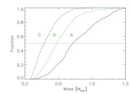
Figure 3: Cumulative distribution of masses in the components of the triples ordered from the brightest (A) to the faintest (C).

Masses of the individual components of resolved triples are estimated from the absolute magnitudes $M_{G}$ in the Gaia band using the 1-Gyr solar-metallicity PARSEC isochrone (Bressan et al., 2012). Stars brighter than $M_{G}=2.66$ mag (some of which are evolved) are removed in the process, so all triples have components on the main sequence with masses less than 1.5 $M_{\odot}$ . The lowest stellar mass of 0.08 $M_{\odot}$ corresponds to $M_{G}=16.7$ or $G=21.7$ mag at a distance of 100 pc (distance modulus 5 mag). This is close to the Gaia magnitude limit, so the GCNS samples all stellar masses down to the hydrogen-burning limit. Only 14 triples (3.6 per cent) have their smallest component less massive than 0.1 $M_{\odot}$ . There are known triple brown dwarfs in the field (e.g. DENIS J020529.0-115925 at 20 pc, separations 0$\farcs$4 and 0$\farcs$07) and brown-dwarf twins orbiting more massive stars (e.g. the 0$\farcs$13 brown-dwarf pair at 90″ from HD 97334). However, these triples are not resolved by Gaia and are not present in our sample.

The median absolute magnitude of the GCNS stars $M_{G}=10.8$ (which coincides with the peak of the luminosity function) corresponds to a star of 0.32 $M_{\odot}$ . The median mass of all stars belonging to our wide triples is 0.47 $M_{\odot}$ , so multiples are on average more massive than single stars. The minimum, median, and maximum values of the total (system) mass are 0.35, 1.53, and 3.70 $M_{\odot}$ , respectively.

Figure 3 shows the cumulative distribution of masses labeled as A, B, C in order of decreasing brightness in each triple. The median values are 0.71, 0.49, and 0.29 $M_{\odot}$ , respectively, so the resolved triples studied here are composed mostly of K- and M-type dwarfs. For comparison, I simulated triples selected randomly from the mass function of the GCNS sample. The median masses in the simulated sample are smaller, 0.59, 0.31, and 0.16 $M_{\odot}$ . The ratios of median tertiary to median primary masses are 0.27 and 0.41 in the simulated and real samples, respectively. This result extends to triples the property of wide binaries to have non-random masses (El-Badry et al., 2019).

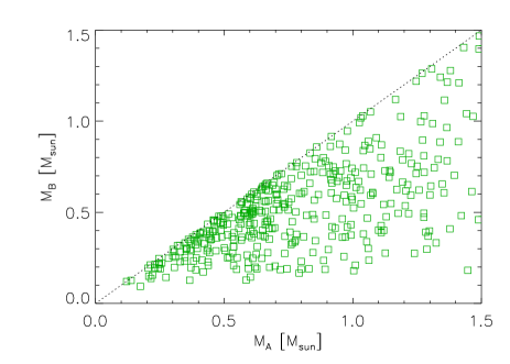
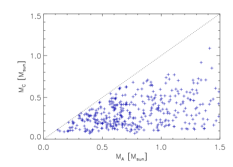
Figure 4: Relation between masses of the brightest star A and the second brightest star B (top) or the dimmest star C (bottom). The dotted line corresponds to mass equality.

The plots in Figure 4 compare masses of the components B and C with the mass of the largest component A. The two most massive components A and B often are similar (twins), as revealed by grouping of the points near the diagonal. The majority of equal-mass pairs belong to the inner subsystems. However, triples where all three stars have similar masses, $M_{C}\approx M_{A}$, are found only at $M_{A}<0.75$ $M_{\odot}$ . The triples studied here are wide (inner separations $\sim$100 au). Close (e.g. spectroscopic) triples with three nearly-equal solar-mass components are quite common, and their absence at large separations tells us something about formation of hierarchical systems.

2.5 Kinematics of Resolved Triples

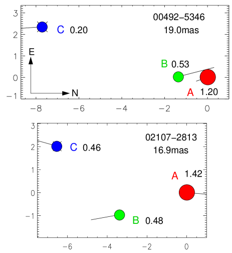
Figure 5: Two resolved triples on the sky, scale in arcseconds. The red, green, and blue circles denote stars in order of decreasing mass, the masses are indicated by numbers. Lines coming from each star show its relative PM, reaching $\sim$5 mas yr^-1in both cases. The WDS codes and mean parallaxes are indicated.

Placing the most massive star A at the coordinate origin, I compute the rectangular X,Y coordinates of other stars (X directed North, Y East) and the differential PMs after subtracting the common center-of-mass PM. Figure 5 illustrates two triples. The first is quite typical, the second has comparable separations and appears as non-hierarchical. Given the coordinates, pairwise distances between the stars are computed. The closest pair is considered as inner (independently of masses), and the remaining star is the tertiary component. This sets the inner and outer separations $\rho$ in arcseconds and the corresponding position angles $\theta$. The angles are counted counter-clockwise from North. The median inner and outer angular separations are 151 and 2570 au, respectively.

The differential PM in the inner pair serves to compute the magnitude $\Delta\mu$ and the position angle $\theta_{\mu}$ of the relative motion vector (secondary relative to primary). The angle $\gamma$ of the relative motion with respect to the pair’s position angle is $\gamma=\theta_{\mu}-\theta$. This angle is defined in the full $360^{\circ}$ range. Values between 0 and $180^{\circ}$ indicate direct (counter-clockwise) orbital motion, small $\gamma$ means a radial motion with increasing separation, while $\gamma\approx 90^{\circ}$ or $\gamma\approx 270^{\circ}$ imply orthogonal motion. Referring to the top panel of Fig. 5, the inner close pair has $\theta=178.5^{\circ}$ and $\gamma=196.8^{\circ}$ (stars approach each other and move clockwise). Using the center of mass of the inner pair, the same parameters, relative position and $\gamma$, are computed for the outer subsystem. In this case, $\gamma=21.9^{\circ}$, meaning that the third star moves away and the outer pair moves counter-clockwise. The median errors of $\gamma$ are 1$\fdg$2 and 2$\fdg$9 in the inner and outer subsystems, respectively. Only 10 triples have errors of outer $\gamma$ exceeding $30^{\circ}$. They are not removed from the statistical analysis to avoid potential bias.

Table 1: Data on resolved wide triple systems (fragment)

$N$	WDS	$\varpi$	Comp.	EDR3	$G$	$M$	$\rho$	$\theta$	$\gamma$	$\sigma_{\gamma}$	$\Delta\mu$	$\mu^{\prime}$
	(J2000)	(mas)			(mag)	($M_{\odot}$ )	(′′)	(deg)	(deg)	(deg)	(mas yr-1)
12	00492-5346	18.84	A	4921910067405272320	7.46	1.20
12		19.19	B	4921910067405761024	12.41	0.54	1.36	178.5	196.9	2.3	5.62	0.30
12		18.83	C	4921910063109280896	15.83	0.20	7.65	162.2	21.9	4.3	3.55	0.43
42	02107-2813	16.94	A	5117251502218279552	6.80	1.42
42		16.81	C	5117251502218710784	13.41	0.46	3.50	195.9	347.6	0.6	6.96	0.69
42		17.00	B	5117251502217614848	13.21	0.48	6.12	158.4	7.9	0.4	6.32	0.74

2.6 Description of the Catalog

Relevant data on the 392 wide triple systems are given in the electronic Table 1. Its fragment reproduced in the text refers to the triples in Figure 5. The first column contains the internal sequential number of the system, replicated in the two following lines (three lines per system: inner primary, inner secondary, and tertiary). The WDS code in column (2) is based on the J2000 coordinates of the brightest star, as in the Washington Double Star catalog (Mason et al., 2001). Column (3) contains the parallaxes of the stars, column (4) gives the mass-related component labels A, B, or C. The Gaia EDR3 identifiers in column (5) provide links to the Gaia and GCNS catalogs, so there is no need to repeat the full astrometric information here. For reference, $G$ magnitudes and estimated masses are given in columns (6) and (7), respectively. The remaining columns are empty for the inner primary. For the inner secondary and the tertiary, they contain separation $\rho$ (8), position angle $\theta$ (9), angle $\gamma$ (10), its error (11), relative motion speed $\Delta\mu$ (12), and its normalized equivalent $\mu^{\prime}$ (13) for the inner and outer subsystems. The errors of $\gamma$ are estimated by the simplified formula $\sigma_{\gamma}=57\fdg 3\sigma_{\Delta\mu}/\Delta\mu$, therefore there is no need to provide the errors $\sigma_{\Delta\mu}$.

3 Statistics

3.1 Separation Ratio

Figure 6: Distribution of the separation ratio (dotted line and crosses) and its deconvolution from projections into the ratio of semimajor axes (full histogram). The vertical line shows the minimum semimajor axis ratio of 2.8 allowed by dynamical stability.

Several apparently non-hierarchical triples (see Figure 5) raise concern about their dynamical stability. Figure 6 shows the distribution of the separation ratio, often expressed as $x=\log_{10}s_{\rm out}/s_{\rm in}$. The median ratio is 14.75, or $x=1.17$. Wide triples cataloged in the MSC (Tokovinin, 2018) have median $x=1.33$, and some of them also appear as non-hierarchical. The distribution of the projected separations can be deconvolved from projections following the recipe described in the Appendix of the MSC paper, converting it into the distribution of the semimajor axis ratio. As expected, it is more compact than the distribution of the separation ratio. The right-hand side of the distribution is shaped by the selection (large ratios are cut off by the Gaia resolution limit). The left part of the curve implies that some systems may be below the minimum ratio of 2.8 (Mardling & Aarseth, 2001). However, this could be caused by the smoothness of the deconvolved distribution, imposed to damp the noise. There is no firm evidence that truly unstable triples are present in the field; such systems decay rapidly. However, existence of many marginally stable wide triples is unquestionable.

3.2 Relative sense of orbital motion and mutual inclination

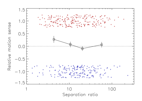
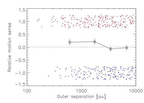
Figure 7: Relative sense of orbital motion vs. separation ratio (top) and outer separation (bottom). The values of +1 and $-$1 correspond to matching and opposite directions of motion, respectively. The symbols are randomly displaced vertically to avoid overlap. The squares with error bars are sign correlations $C$ computed for quarters of the sample.

The inner and outer angles $\gamma$ define the sense of revolution in these triples, allowing some inference on the mutual orbit alignment. Of the 392 triples, $N_{+}=211$ revolve in the same sense. The sign correlation $C=(N_{+}-N_{-})/(N_{+}+N_{-})$ is $0.076\pm 0.050$. This parameter is related to the mean mutual inclination $\Phi=90^{\circ}(1-C)=83\fdg 1\pm 4\fdg 5$. In a sample of 216 visual triples from the MSC, a significant degree of orbit alignment has been found at outer separations below 50 au, while triples wider that 1000 au had random mutual inclinations (Tokovinin, 2017). To probe potential dependence of mutual orbit alignment in wide triples on the separation ratio and outer separation, I plot in Figure 7 the relative motion sense (positive and negative numbers for triples with orbital motion in the same and opposite sense, respectively) vs. these parameters. The sample was split over each parameter into four equal groups, and $C$ was computed for each group (squares with error bars). One can see that more compact triples seem to have a weak (although not statistically significant) alignment, while wide triples definitely have randomly oriented orbits. This confirms the tendency found in the MSC and extends it to wider separations, thanks to the accurate Gaia astrometry.

3.3 Eccentricities

Figure 8: Plots of $\gamma^{\prime}$ vs. $\mu^{\prime}$ for the inner (top) and outer (bottom) subsystems.

The joint distribution of $(\mu^{\prime},\gamma^{\prime})$ allows to reconstruct the eccentricity distribution, as demonstrated by Tokovinin & Kiyaeva (2016) and Tokovinin (2020). Here $\gamma^{\prime}=\arcsin(|\sin(\gamma)|)$ is the angle folded into the $(0,90^{\circ})$ interval. Figure 8 shows these plots for the inner and outer subsystems. Although the number of points is modest, one notes that values $\gamma^{\prime}\sim 90^{\circ}$ are more frequent in the outer pairs. Similar plots simulated for binaries with fixed eccentricities easily distinguish between circular and eccentric orbits. Table 2 gives the median values of the parameters (the errors are determined by bootstrap) and their correlation coefficients $\rho_{\mu\gamma}$. Its last two columns give these values for the thermal and uniform eccentricity distributions, as determined by Tokovinin & Kiyaeva (2016). For reference, $e=0.8$ corresponds to median $\gamma^{\prime}=41\fdg 4$ and a strong anti-correlation $\rho_{\mu\gamma}=-0.21$.

Table 2: Statistics of relative motion

Parameter	Inner	Outer	$f(e)=2e$	$f(e)=1$
Median $\gamma^{\prime}$	50.4$\pm$2.2	53.3$\pm$2.6	45.0	53.5
Median $\mu^{\prime}$	0.52$\pm$0.04	0.64$\pm$0.02	0.546	0.608
$\rho_{\mu\gamma}$	0.04	0.15	0	0.08

Figure 9: Cumulative distributions of angles $\gamma^{\prime}$ in the inner and outer subsystems. The dotted line corresponds to the uniform distribution.

Table 3: Eccentricity distributions

Case	$f_{1}$	$f_{2}$	$f_{3}$	$f_{4}$	$f_{5}$	$f_{6}$	$f_{7}$	$f_{8}$	$f_{9}$	$f_{10}$
Inner $f_{i}$	0.028	0.017	0.019	0.048	0.093	0.141	0.177	0.182	0.160	0.135
Inner $f_{\rm med}$	0.010	0.020	0.035	0.062	0.097	0.133	0.161	0.174	0.168	0.138
Inner $\sigma_{f}$	0.013	0.010	0.012	0.015	0.016	0.016	0.017	0.017	0.017	0.025
Outer $f_{i}$	0.031	0.018	0.019	0.047	0.087	0.133	0.174	0.183	0.161	0.147
Outer $f_{\rm med}$	0.010	0.021	0.037	0.063	0.095	0.128	0.156	0.170	0.175	0.144
Outer $\sigma_{f}$	0.013	0.010	0.013	0.015	0.017	0.018	0.019	0.018	0.017	0.024
Outer simulated	0.023	0.070	0.118	0.143	0.142	0.175	0.163	0.114	0.051	0.001

Figure 9 shows cumulative distributions of the angles $\gamma^{\prime}$. For the inner subsystems, it is closer to uniform (dotted line), while for the outer systems it is consistently below. The maximum difference with the uniform distribution for the outer systems, 0.110, corresponds to the Kolmogorov-Smirnov significance level of 0.00012. The thermal distribution of outer eccentricities is definitely rejected.

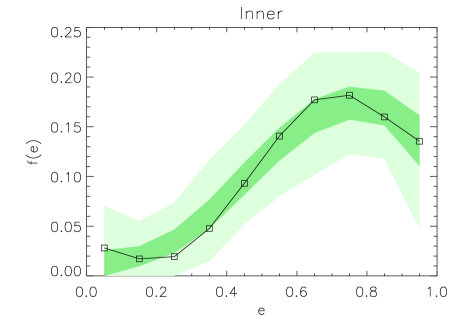
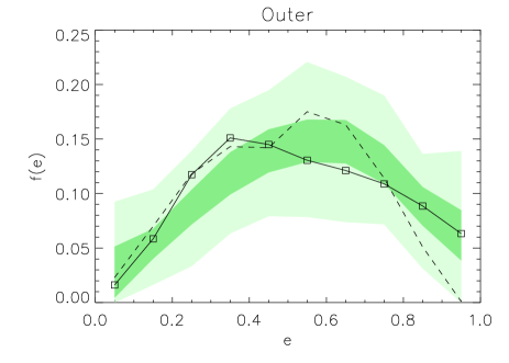
Figure 10: Eccentricity distributions in the inner (top) and outer (bottom) subsystems derived from the $(\mu^{\prime},\gamma^{\prime})$ statistics (squares and full line). The light and dark green shadings show the full and $\pm\sigma$ range of bootstrap results. The dashed line in the lower plot is the eccentricity distribution expected from the dynamical stability constraint.

The eccentricity distributions were derived from the $(\mu^{\prime},\gamma^{\prime})$ arrays by the algorithm described in Tokovinin (2020). Briefly, the observed histogram is modeled by a linear combination of simulated histograms (templates) with coefficients $f_{i}$. The templates are derived for simulated binaries with a narrow range of eccentricities, all other orbital parameters being random. I use 10 templates corresponding to 0.1 eccentricity intervals. The fitted parameters $f_{i}$ are non-negative and satisfy the condition $\sum_{i}f_{i}=1$. A small regularization parameter $\alpha$ is introduced to reduce the noise. After a few trials, I selected $\alpha=0.01$; $\alpha=0.1$ is too large, biasing the result toward uniform distribution, while $\alpha=0.001$ gives noisy results. The errors of the derived distributions are estimated by bootstrap: the data are randomly re-sampled 1000 times and the reconstruction of the eccentricity distribution is repeated.

The eccentricity distributions of the inner and outer orbits determined by this method are given in Table 3 and plotted in Figure 10. The values $f_{i}$ (squares connected by the full line) are obtained directly from the data. The full range of values obtained by bootstrap is shown by the light green color, while the darker green marks the 68 percentile of the distribution. Half of this range gives estimates of the errors $\sigma_{f}$ and is listed in Table 3 together with the bootstrap medians $f_{\rm med}$.

The bootstrap analysis gives the confidence intervals of the derived distributions (which, however, depend on $\alpha$). The initial decreasing part of the inner eccentricity distribution is likely a result of random errors because the bootstrap medians demonstrate only a smooth growth. However, the decline at $e_{\rm in}>0.8$ is a robust feature. Interestingly, a similar decline was found by Tokovinin & Kiyaeva (2016) for wide solar-type binaries (their Figure 7).

The resolution limit of Gaia removes from the sample close inner subsystems and can affect the resulting distribution of $(\mu^{\prime},\gamma^{\prime})$ in a systematic way. To address this concern, I simulated a population of inner binaries by choosing their magnitude differences $\Delta G$ from the empirical distribution for real inner systems wider than 2″, unaffected by the Gaia limit. The semimajor axis was chosen from a log-uniform distribution between 10 and 330 au, the distances match the actual distance distribution. Binaries that happened to be below the Gaia separation-contrast limit were removed. The bottom panel of Figure 2 compares simulated and real inner subsystems. The template distributions used in the reconstruction of $f(e)$ for the inner subsystems were derived from those simulated inner binaries ($10^{4}$ per eccentricity interval). However, the result turned out to be almost identical to the standard reconstruction that used generic templates without resolution cutoff. The reconstructed distribution of inner eccentricities thus appears robust. The mean inner eccentricity is $e_{\rm in}=0.66\pm 0.02$.

The distribution of outer eccentricities in Table 3 and Figure 10 is markedly different from the inner one and corresponds to the mean eccentricity of $e_{\rm out}=0.54\pm 0.02$. This result is also robust and confirms previous studies: outer orbits in hierarchies are less eccentric compared to binaries of similar separations (Shatsky, 2001; Tokovinin & Kiyaeva, 2016). This is natural because eccentric outer orbits are not allowed by dynamical stability, especially for our wide triples with moderate separation ratios. I show below that dynamical stability can indeed explain the observed paucity of eccentric outer orbits.

A large number of outer orbits with a thermal eccentricity distribution was simulated and unstable systems were removed. The stability criterion of Mardling & Aarseth (2001) requires the ratio of semimajor axes $r=a_{\rm out}/a_{\rm in}$ to be larger than the critical ratio $r_{\rm crit}$,

$$r_{\rm crit}=2.8(1+q_{\rm out})^{1/15}(1+e_{\rm out})^{0.4}(1-e_{\rm out})^{-1.2}.$$ (2)

For each system, a random semimajor axis ratio was generated in agreement with the histogram in Figure 6. The median outer mass ratio $q_{\rm out}=0.4$ was adopted. The resulting outer eccentricity distribution of the remaining stable triples (dashed line in the lower panel of Figure 10 and the last line of Table 3) resembles the actual distribution of outer eccentricities. The two curves do not match exactly because of simplifying assumptions adopted in the simulations. I also used this simulated $f(e)$ to generate a simulated $(\mu^{\prime},\gamma^{\prime})$ plot. The median values from this simulation ($\gamma^{\prime}=56\fdg 2$, $\mu^{\prime}=0.61$, $\rho_{\mu\gamma}=0.18$) are in rough agreement with the measured values for outer pairs in Table 2. Thus, the dynamical stability limit appears to be the primary cause of rounded outer orbits in the resolved triples with moderate separation ratios.

The dynamical stability allows outer orbits in wide triples to become more eccentric at increasing outer separation. Splitting the sample into three groups by the outer separation (below 1 kau, $N$=85; between 1 and 3 kau, $N$=135; and above 3 kau, $N$=168), I find the decreasing median $\gamma^{\prime}$ (58$\fdg$5, 56$\fdg$3, and 49$\fdg$7, respectively). However, even at the largest separations, the outer eccentricity distribution appears to be softer than the thermal one.

3.4 Mass ratios

Figure 11: Mass ratio vs. projected separation in the inner (top) and outer (bottom) subsystems. The dashed line in the top panel illustrates the Gaia detection limit at 100 pc distance. Squares (crosses) denote systems with primaries more (less) massive than 0.75 $M_{\odot}$ .

The mass ratios give additional insight on the formation of these triples. The inner mass ratio $q_{\rm in}=M_{2}/M_{1}$ cannot exceed one by definition, while the outer mass ratio $q_{\rm out}=M_{3}/(M_{1}+M_{2})$ can be larger than one. The masses are arranged by hierarchy, not sorted in decreasing order. In the top panel of Figure 11, we see a clear trend caused by the Gaia detection limit (high-contrast pairs at small separations are not recognized as distinct sources). The dotted line represents this limit (according to eq. 2 in GCNS) at a distance of 100 pc, converted into mass ratio for a solar-mass primary. At closer distance, this curve is displaced to the left. The envelope of the points follows the slope of the detection curve quite well. The median values of the inner and outer mass ratios are 0.76 and 0.41, respectively. When the sample is split around the primary mass of 0.75 $M_{\odot}$ , the median inner and outer mass ratios for the low-mass part are 0.82 and 0.42, while for the high-mass part they are slightly smaller, 0.68 and 0.39. For the 224 triples with inner separation above 2″, little affected by the Gaia detection limit, the median inner mass ratio is still high, 0.64.

Figure 12: Histogram of inner mass ratios.

A large number of inner twins with $q_{\rm in}>0.95$ is obvious and it is not a selection effect, as can be appreciated in the histogram of Figure 12. The excess of 46 systems in the last bin, compared to the preceding one, implies the inner twin fraction of $f_{\rm twin}=46/392=0.12$ according to the definition of this parameter in Moe & Di Stefano (2017). The total fraction of inner subsystems with $q_{\rm in}>0.95$ is 82/392=0.21. Existence of wide twin binaries in the field has been convincingly demonstrated by El-Badry et al. (2019). Their Figure 10 gives the average $f_{\rm twin}=0.12$ for the separation range of 50–350 au and masses from 0.1 to 0.8 $M_{\odot}$ , similar to the fraction found here for inner subsystems.

The outer mass ratios are not biased by the Gaia detection limit. One can discern in the bottom panel of Figure 11 a weak trend of decreasing outer mass ratios with increasing separation. Splitting the sample around 2.7 kau, one finds the median $q_{\rm out}$ of 0.46 and 0.34 for the closer and wider triples, respectively.

Figure 13: Relation between inner and outer mass ratios. Crosses and squares denote triples with primary masses below and above 0.75 $M_{\odot}$ , respectively. The line corresponds to $M_{1}=M_{3}$.

Figure 13 illustrates the relation between inner and outer mass ratios. The line $q_{\rm out}=1/(1+q_{\rm in})$ corresponds to $M_{1}=M_{3}$ and separates 269 triples where the most massive star resides in the inner pair from 123 systems where the most massive star is the tertiary component. So, only 31 per cent of the triples have the hierarchy of A-BC type (a low-mass inner pair and a more massive tertiary), while the majority are of AB-C type or AC-B types where the most massive star A belongs to the inner pair. Focusing on the 82 inner twins with $q_{\rm in}>0.95$, one finds the median $q_{\rm out}=0.51$, larger than in the full sample. In half of the triples with inner twins, the tertiary is the most massive star. In the remaining 310 triples without inner twins ($q_{\rm in}<0.95$), the fraction of massive tertiaries is 82/310=0.26. Thus, we note some correlation between inner and outer mass ratios.

4 Origin of Wide Triples

Formation of wide hierarchies by turbulent core fragmentation has been studied by hydrodynamic simulations in several papers. Lee et al. (2019) show how wide systems with separations of $\sim$10 kau form and fall to the common center of mass while still accreting. Those wide pairs are not yet binaries because they have not completed one full orbit (the estimated orbital periods exceed their age). Eventually, they settle into closer orbits. Migration from wide to close separations is driven by two factors: mass accretion and dynamical gas friction. Unstable groups of three or more stars form frequently and most of them disintegrate, ejecting preferentially low-mass members (orphans); swaps between components of hierarchies are also frequent. Lee et al. estimate that a 0.8 fraction of all stars belonged to systems at some point in their history, even though the final multiplicity fraction is only about 0.5. Components of binaries and multiples are more massive than orphans and single stars (those that never belonged to any system).

We see that components of wide triples in the field are, on average, more massive than single stars, in agreement with these simulations. This means that they have accreted a substantial mass, and, consequently, their orbits have been modified by accretion. The stellar system mass function (SMF) has a broad peak around 0.2-0.3 $M_{\odot}$ and a power-law tail at higher masses. The SMF can be modeled by assuming that low-mass stars representing the SMF peak are produced by core collapse, and the high-mass tail results from competitive accretion onto these low-mass seeds (Clark & Whitworth, 2021). From this perspective, our triples with a median system mass of 1.53 $M_{\odot}$ belong to the high-mass SMF tail. A substantial fraction of inner twins points to the same conclusion because twins are produced by preferential growth of secondary components in accreting binaries. A binary that formed early and subsequently accreted a major fraction of its mass has a high probability to become a twin. The ‘twin syndrome’, typical for close binaries (Tokovinin & Moe, 2020), also exists at separations on the order of 1 kau and beyond, as shown by El-Badry et al. (2019). Formation of low-mass stars by core collapse produced many twin binaries and multiple systems in the hydrodynamical simulations by Rohde et al. (2021): their Figure 9 qualitatively resembles the histogram of inner mass ratios in Figure 12, showing a preference for large $q$ and a prominent twins peak. Lomax et al. (2015) also predicted preferentially large mass ratios. However, in both works separations of simulated systems are smaller compared to our wide field triples.

The second important conclusion from these simulations is the importance of dynamical interactions in nascent stellar systems. They often contain three or more stars in non-hierarchical configurations that decay by ejecting orphans. The surviving hierarchies are dynamically stable, but not too far from the stability limit. Their orbits are not aligned, unless the initial configuration was highly flattened and had a substantial angular momentum (Sterzik & Tokovinin, 2002). In the numerical scattering experiments where a binary or a triple system interacts with a passing single or binary star, the resulting triples are always near the limit of dynamical stability, their mutual orbit orientation is random, and the inner eccentricities have a thermal distribution (Antognini & Thompson, 2016).

Wide triples in the field match the products of dynamical decay in several respects: their separations are comparable, the mutual orbit orientation is almost random, and the inner eccentricities are large. However, the distribution of inner eccentricities in Figure 10 is not quite thermal, flattening and declining at $e_{\rm in}>0.7$. This can be explained by dissipative interaction with gas near the periastrons of very eccentric inner orbits that reduces eccentricities to moderate values and contributes to the broad peak at $e_{\rm in}\sim 0.7$. In the more compact visual triples studied by Tokovinin (2017), the inner eccentricities are even smaller (median 0.5), and there is a clear tendency to mutual orbit alignment at outer separations less than 1 kau. These observations point to the dynamical importance of gas at separations below $\sim$100 au. In the simulations by Lomax et al. (2015), triples with aligned orbits and moderate eccentricities were produced owing to the energy dissipation in gas. On the other hand, moderate eccentricities of the outer orbits in wide triples are a simple consequence of the N-body dynamics: only stable triples have survived.

Motions in an unstable triple lead to ejections of one star (usually the smallest) to large separations. If the system remains bound, the ejected star returns, and the system eventually disintegrates. However, interactions with gas modify this picture by shrinking the inner orbit, which may render the system dynamically stable. Interactions of the ejected star with other nearby stars can also stabilize the system by supplying additional angular momentum to the outer orbit. Most wide dynamically stable triples formed by ejections (unfolding) have eccentric outer orbits (Reipurth & Mikkola, 2012). In contrast, wide triples in the field have moderate outer eccentricities, hence the unfolding mechanism has not contributed to their formation in any significant way. The mass ratios of wide field triples do not match the predictions of Reipurth & Mikkola (2015) when we compare Figure 13 with their Figure 14.

Large outer separations of the triples studied here indicate that these systems have not experienced disruptive interactions in dense clusters but rather formed in low-density environments like Taurus-Auriga. The plot in Figure 11 suggests that outer separations extend well beyond the 10 kau cutoff imposed here. Joncour et al. (2017) discovered in Taurus a population of ultra-wide binaries with separations up to 60 kau, the majority of them hosting inner subsystems with separations below 1 kau. At projected separations from 1 to 10 kau, hierarchical multiples in Taurus outnumber simple wide binaries. These authors determined that stars belonging to hierarchies are more massive than single stars; components less massive than 0.1 $M_{\odot}$ are rare, while typical masses in hierarchies are 0.6-0.8 $M_{\odot}$ . Joncour et al. give convincing arguments that wide hierarchies in Taurus are pristine products of the cascade (hierarchical) collapse of elongated cores. These multiples will evolve to closer separations (as in the simulations of Lee et al., 2019), some of them will decay dynamically, and the surviving systems will possibly resemble the wide triples in the field.

5 Summary

Here are the main results of this study in a condensed form.

• A sample of 392 wide low-mass triples within 100 pc resolved by Gaia is selected, masses and internal motions in these systems are determined. Most triples contain only three stars, although undetected inner subsystems cannot be fully excluded. The sample is complete above the Gaia separation-contrast limit; it represents a 0.0012 fraction of the total field population. The median primary mass is 0.71 $M_{\odot}$ , and all components of these triples are more massive than average field stars.

• The median inner and outer separations are 151 and 2570 au, respectively, and their median ratio is 14.75, signaling that many wide triples are just above the dynamical stability limit. The outer projected separations are restricted here to be $<$10 kau, but wider triples certainly exist in the field.

• The inner and outer orbits are aligned almost randomly with the average mutual inclination of $83\fdg 1\pm 4\fdg 5$.

• The direction and velocity of relative motion is used here to infer the eccentricity distributions. The mean inner eccentricity is 0.66$\pm$0.02; its distribution resembles a thermal one, but flattens and declines at $e_{\rm in}>0.7$. The smaller mean outer eccentricity of 0.54$\pm$0.02 can be explained by the combination of dynamical stability and moderate separation ratios that effectively remove eccentric outer orbits from the sample.

• The inner mass ratios are typically large (median 0.64 at inner separation above 2″), and a 0.21 fraction of inner binaries are twins with $q_{\rm in}>0.95$ (twin excess of 0.12). The median outer mass ratio $q_{\rm out}=0.41$ has a weak trend of decreasing with outer separation. Only in 31 per cent of wide triples the most massive star is a tertiary component.

• Young wide hierarchies in Taurus studied by Joncour et al. (2017), likely formed by a cascade (hierarchical) collapse of elongated cores, could be progenitors of wide triples in the field.

The present sample of wide triples represents only a tiny fraction of all hierarchical systems within 100 pc. Assuming that 5 per cent of stars more massive than 0.3 $M_{\odot}$ (the median mass) belong to hierarchies, their total number within 100 pc can be as large as 8 000, twenty times more than this sample. Inner pairs in most of these hierarchies are not resolved by Gaia, but their presence can be often guessed from the increased astrometric noise or variable RVs. Periods and mass ratios in these hypothetical subsystems remain, so far, unknown. Future Gaia data releases will enrich the 100-pc sample by adding close resolved binaries and providing astrometric and spectroscopic orbits for some subsystems. Still, a tremendous work remains to be done to complement Gaia by high-resolution imaging and RV monitoring from the ground. Statistical study of typical, more compact hierarchical systems will help us to reveal the mystery of their formation.

References

- Antognini & Thompson (2016) Antognini, J. M. O., & Thompson, T. A. 2016, MNRAS, 456, 4219, doi: 10.1093/mnras/stv2938
- Bate (2014) Bate, M. R. 2014, MNRAS, 442, 285, doi: 10.1093/mnras/stu795
- Bressan et al. (2012) Bressan, A., Marigo, P., Girardi, L., et al. 2012, MNRAS, 427, 127, doi: 10.1111/j.1365-2966.2012.21948.x
- Clark & Whitworth (2021) Clark, P. C., & Whitworth, A. P. 2021, MNRAS, 500, 1697, doi: 10.1093/mnras/staa3176
- Duchêne & Kraus (2013) Duchêne, G., & Kraus, A. 2013, ARA&A, 51, 269, doi: 10.1146/annurev-astro-081710-102602
- El-Badry et al. (2021) El-Badry, K., Rix, H.-W., & Heintz, T. M. 2021, MNRAS, 506, 2269, doi: 10.1093/mnras/stab323
- El-Badry et al. (2019) El-Badry, K., Rix, H.-W., Tian, H., Duchêne, G., & Moe, M. 2019, MNRAS, 489, 5822, doi: 10.1093/mnras/stz2480
- Gaia Collaboration et al. (2016) Gaia Collaboration, Brown, A. G. A., Vallenari, A., et al. 2016, A&A, 595, A2, doi: 10.1051/0004-6361/201629512
- Gaia Collaboration et al. (2021a) —. 2021a, A&A, 649, A1, doi: 10.1051/0004-6361/202039657
- Gaia Collaboration et al. (2021b) Gaia Collaboration, Smart, R. L., Sarro, L. M., et al. 2021b, A&A, 649, A6, doi: 10.1051/0004-6361/202039498
- Joncour et al. (2017) Joncour, I., Duchêne, G., & Moraux, E. 2017, A&A, 599, A14, doi: 10.1051/0004-6361/201629398
- Lee et al. (2019) Lee, A. T., Offner, S. S. R., Kratter, K. M., Smullen, R. A., & Li, P. S. 2019, ApJ, 887, 232, doi: 10.3847/1538-4357/ab584b
- Lomax et al. (2015) Lomax, O., Whitworth, A. P., Hubber, D. A., Stamatellos, D., & Walch, S. 2015, MNRAS, 447, 1550, doi: 10.1093/mnras/stu2530
- Mardling & Aarseth (2001) Mardling, R. A., & Aarseth, S. J. 2001, MNRAS, 321, 398, doi: 10.1046/j.1365-8711.2001.03974.x
- Mason et al. (2001) Mason, B. D., Wycoff, G. L., Hartkopf, W. I., Douglass, G. G., & Worley, C. E. 2001, AJ, 122, 3466, doi: 10.1086/323920
- Moe & Di Stefano (2017) Moe, M., & Di Stefano, R. 2017, ApJS, 230, 15, doi: 10.3847/1538-4365/aa6fb6
- Raghavan et al. (2010) Raghavan, D., McAlister, H. A., Henry, T. J., et al. 2010, ApJS, 190, 1, doi: 10.1088/0067-0049/190/1/1
- Reipurth & Mikkola (2012) Reipurth, B., & Mikkola, S. 2012, Nature, 492, 221, doi: 10.1038/nature11662
- Reipurth & Mikkola (2015) —. 2015, AJ, 149, 145, doi: 10.1088/0004-6256/149/4/145
- Rohde et al. (2021) Rohde, P. F., Walch, S., Clarke, S. D., et al. 2021, MNRAS, 500, 3594, doi: 10.1093/mnras/staa2926
- Shatsky (2001) Shatsky, N. 2001, A&A, 380, 238, doi: 10.1051/0004-6361:20011401
- Sterzik & Tokovinin (2002) Sterzik, M. F., & Tokovinin, A. A. 2002, A&A, 384, 1030, doi: 10.1051/0004-6361:20020105
- Tokovinin (2014) Tokovinin, A. 2014, AJ, 147, 86, doi: 10.1088/0004-6256/147/4/86
- Tokovinin (2017) —. 2017, ApJ, 844, 103, doi: 10.3847/1538-4357/aa7746
- Tokovinin (2018) —. 2018, ApJS, 235, 6, doi: 10.3847/1538-4365/aaa1a5
- Tokovinin (2020) —. 2020, MNRAS, 496, 987, doi: 10.1093/mnras/staa1639
- Tokovinin & Kiyaeva (2016) Tokovinin, A., & Kiyaeva, O. 2016, MNRAS, 456, 2070, doi: 10.1093/mnras/stv2825
- Tokovinin & Moe (2020) Tokovinin, A., & Moe, M. 2020, MNRAS, 491, 5158, doi: 10.1093/mnras/stz3299
- Winters et al. (2019) Winters, J. G., Henry, T. J., Jao, W.-C., et al. 2019, AJ, 157, 216, doi: 10.3847/1538-3881/ab05dc