Dijkstra’s Algorithm with Predictions to Solve the Single-Source Many-Targets Shortest-Path Problem

Abstract

We study the use of machine learning techniques to solve a fundamental shortest path problem, known as the single-source many-targets shortest path problem (SSMTSP). Given a directed graph with non-negative edge weights, our goal is to compute a shortest path from a given source node to any of several designated target nodes. Basically, our idea is to equip an adapted version of Dijkstra’s algorithm with machine learning predictions to solve this problem: Based on the trace of the algorithm, we design a neural network that predicts the shortest path distance after a few iterations. The prediction is then used to prune the search space explored by Dijkstra’s algorithm, which may significantly reduce the number of operations on the underlying priority queue. We note that our algorithm works independently of the specific method that is used to arrive at such predictions. Crucially, we require that our algorithm always computes an optimal solution (independently of the accuracy of the prediction) and provides a certificate of optimality. As we show, in the worst-case this might force our algorithm to use the same number of queue operations as Dijkstra’s algorithm, even if the prediction is correct. In general, however, our algorithm may save a significant fraction of the priority queue operations. We derive structural insights that allow us to lower bound these savings on partial random instances. In these instances, an adversary can fix the instance arbitrarily except for the weights of a subset of relevant edges, which are chosen randomly. Our bound shows that the number of relevant edges which are pruned increases as the prediction error decreases. We then use these insights to derive closed-form expressions of the expected number of saved queue operations on random instances. We also present extensive experimental results on random instances showing that the actual savings are oftentimes significantly larger.

1 Introduction

In recent years, techniques from machine learning (ML) have proven extremely powerful to tackle problems that were considered to be very difficult or even unsolvable. Success stories include contributions to health care, natural language processing, image recognition, board games, etc. (see, e.g., Chugh et al. (2021); Lu and Weng (2007); Otter et al. (2020); Qayyum et al. (2020); Silver et al. (2018, 2017)). As such, machine learning is intimately connected with optimisation because many learning algorithms are based on the optimisation of some loss function over a large set of training samples. Even though optimisation techniques play a vital role in the design of ML-approaches, the reverse direction of using ML-techniques to improve optimisation algorithms is much less explored.

In this paper, we contribute to the emerging research agenda of studying how ML-approaches can be used to design improved algorithms for optimisation problems. One research direction along these lines has become known as Algorithms with Predictions (or Learning Augmented Algorithms). This research theme first emerged in the area of online algorithms (see Medina and Vassilvitskii (2017); Kumar et al. (2018); Lykouris and Vassilvitskii (2021)), where it has been studied intensively for several years now. More recently, similar ideas are investigated also in the context of exact algorithms, data structures, equilibrium analysis and mechanism design. An overview of research articles that appeared on these topics is available at https://algorithms-with-predictions.github.io.

In the context of online computation, the idea is to consider online algorithms that can make use of predictions of certain (problem-specific) parameters. For example, such predictions could be obtained from historical input data through the use of machine learning techniques. In fact, these predictions cannot be assumed to be exact as they might be prone to (arbitrarily large) errors. The goal then is to design online algorithms that achieve improved competitive ratios (depending on the quality of the predictions). Along these lines, the following three objectives emerged in the literature (see also Lykouris and Vassilvitskii (2021)): (1) $\alpha$-consistency: If the predictions are perfect (i.e., error-free), the competitive ratio of the online algorithms is bounded by $\alpha$. (2) $\beta$-robustness: Even if the predictions are arbitrarily bad, the competitive ratio of the online algorithm is bounded by $\beta$. Ideally, $\beta$ is not (much) worse than the worst-case competitive ratio known for the problem. (3) $\gamma$-approximate: If the predictions are within an error of $\eta$ of the actual values (for a suitably defined error parameter $\eta)$, the competitive ratio of the online algorithm is bounded by some function $\gamma(\eta)$. Even though the above model was originally introduced for the online setting, it naturally extends to other worst-case performance measures. More recently, researchers started to apply this framework to the study of the running time of algorithms (see, e.g., Dinitz et al. (2021); Chen et al. (2022)), the price of anarchy of equilibria (see, e.g., Gkatzelis et al. (2022)) and the social welfare efficiency of truthful mechanisms (see, e.g., Xu and Lu (2022)).

We investigate the use of predictions in the context of a fundamental shortest path problem, which is known as the single-source many-targets shortest path problem (SSMTSP). Given a directed graph $G=(V,E)$ with non-negative edge weights $w:E\rightarrow\mathbb{R}_{\geq 0}$, a source node $s\in V$ and a subset $T\subseteq V$ of designated target nodes, the goal is to compute a shortest path from $s$ to any of the target nodes in $T$. Note that the SSMTSP problem generalises the single-source single-target shortest path problem (for which $T=\{t\}$ for a given target node $t\in V$) and the single-source all-targets shortest path problem (for which $T=V$). These shortest path problems are among the most fundamental optimisation problems with various applications in practice. Further, both the assignment problem and the maximum weight matching problem in bipartite graphs can be reduced to the solving of $n$ SSMTSP problems, where $n$ is the maximum number of nodes on each side of the bipartition (see, e.g., Bast et al. (2003) for details). Clearly, this emphasises the importance of deriving efficient algorithms for this problem.

The SSMTSP problem can be solved exactly in (strongly) polynomial time by using a slight adaption of the well-known shortest path algorithm due to Dijkstra (1959) (subsequently referred to as Dijkstra). Basically, Dijkstra grows a shortest path tree rooted at the source node $s$ by iteratively adding new nodes to the tree by increasing distances, until the first target node from $T$ is included. Dijkstra guarantees a worst-case running time of $O(m+n\log n)$, where $n$ and $m$ denote the number of nodes and edges, respectively. In order to achieve this running time, crucially the underlying priority queue data structure must be implemented through Fibonacci heaps (see Fredman and Tarjan (1987)). In terms of worst-case running time, Dijkstra is the best known algorithm that runs in strongly polynomial time for the shortest path problem with arbitrary non-negative edge weights (see, e.g., Cormen et al. (2009)). If the edge weights are known to be non-negative integers from a restricted range, there are better algorithms (see also the related work section).

Given that the SSMTSP problem can be solved very efficiently by Dijkstra’s algorithm, it is unclear how predictions can help to further improve the running time of the algorithm. In this paper, we focus on exact algorithms for the SSMTSP problem. More specifically, we require that the algorithm computes a shortest path together with a certificate that proves optimality, even if the predictions are arbitrarily bad. A common approach to exhibit such a certificate is by means of a corresponding dual solution to the linear programming formulation of the problem. The single-source single-target shortest path problem has a natural (flow-based) linear programming formulation (see, e.g., Papadimitriou and Steiglitz (1998)). The dual of this linear program associates a dual variable $\pi(u)$ with every node $u\in V$ and reads as follows:

$$\max\quad\pi(t)-\pi(s)\quad\text{subject to}\quad\pi(v)\leq\pi(u)+w(u,v)\ \ \ \forall(u,v)\in E.$$ (D)

In this formulation, we can fix $\pi(s)=0$ without loss of generality. The respective dual values then have a natural interpretation as shortest path distances. By applying the complementary slackness condition, a dual feasible solution $\pi=(\pi_{u})_{u\in V}$ proves the optimality of an $s,t$-path if and only if every edge $e=(u,v)$ on that path is tight, i.e., $\pi(v)=\pi(u)+w(u,v)$. Most exact shortest path algorithms known in the literature provide a certificate of optimality by constructing such an optimal dual solution (or, equivalently, shortest path distances).

Chen et al. (2022) recently studied algorithms with predictions for the single-source shortest path problem with arbitrary edge weights under the assumption that a (possibly infeasible) dual solution $\hat{\pi}=(\hat{\pi}(u))_{u\in V}$ is available as prediction. Note that this predictions consists of $n=|V|$ dual values. Building on earlier work by Dinitz et al. (2021), they show that such predictions can be used to obtain an algorithm to solve this problem in time $O(m\min\{\|\hat{\pi}-\pi^{*}\|_{1}\cdot\|\hat{\pi}-\pi^{*}\|_{\infty},\sqrt{n}\log(\|\hat{\pi}-\pi^{*}\|_{\infty})\})$, where $\pi^{*}$ is an optimal dual solution to the problem. In particular, the worst-case running time improves as the difference (evaluated with respect to the $L_{1}$- and $L_{\infty}$-norm) between the predicted duals $\hat{\pi}$ and the optimal duals $\pi^{*}$ decreases. Clearly, such results are appealing as they provide a fine-grained running time guarantee depending on the (cumulative) additive error of the predictions. On the negative side, however, assuming that one has access to the entire dual solution $\hat{\pi}$ might be a rather strong assumption in certain settings—especially because the number of nodes (and thus the number of values to predict) can be very large in practice.

In this paper, we therefore consider the other end of the spectrum: We assume that our algorithm has access to a single predicted value only, namely the shortest path distance of a target node. Said differently, we assume that we have access to a prediction of the objective function value $\hat{\pi}_{t}$ of (D) (which might not necessarily coincide with the optimal objective function value $\pi_{t}^{*}$). The question that we address here is whether such a minimalistic prediction suffices to still achieve a running time improvement of Dijkstra’s algorithm.

Clearly, exploiting a prediction of the shortest path distance only is much more restrictive than assuming that one has access to an entire dual solution—in fact, the latter can be used to derive the former. Intuitively, it is clear that it is more challenging to improve Dijkstra’s algorithm using such an (inferior) prediction. The following observation lends further support to this intuition. Recall that we require that our algorithm provides a certificate of optimality. If the entire dual solution is predicted perfectly, this becomes trivial: the dual itself provides such a certificate and is readily available in this case. On the other hand, this remains a challenging task in our setting: even if the correct shortest path distance is known, it is non-trivial (in terms of computational work) to compute a corresponding dual solution that proves optimality. This latter observation will be made more rigorous in Section 4.

Our algorithm is based on a heuristic improvement of Dijkstra’s algorithm proposed by Bast et al. (2003) (referred to as Dijkstra-Pruning). The key idea of their algorithm is to exploit that Dijkstra’s algorithm might encounter many target nodes in $T$ before the actual target node (defining the shortest path distance) is added to the tree: Dijkstra-Pruning simply keeps track of the smallest distance $B$ to a node in $T$ that was encountered so far. The algorithm then prunes each edge that leads to a node whose distance exceeds $B$—clearly, these edges are irrelevant for the final shortest path. A more detailed description of this algorithm will be given in Section 2. Although the pruning idea is very simple, it can significantly improve the running time of the algorithm. In the worst case, however, Dijkstra-Pruning has the same running time as Dijkstra. Therefore, Bast et al. (2003) investigate the effectiveness of Dijkstra-Pruning on random instances, both analytically and experimentally. They show that the pruning of irrelevant edges significantly reduces the number of executed priority queue operations on these instances.

1.1 Our Contributions

The main contributions presented in this paper are as follows:

1. We combine an ML-approach with the pruning idea above to obtain a new algorithm for the SSMTSP problem. Basically, our algorithm (referred to as Dijkstra-Prediction) computes a prediction $P$ of the final shortest path distance after a few iterations, and then uses this prediction $P$ together with the pruning trick of Bast et al. (2003) to further reduce the search space it explores. On the ML-side, one of the challenges is to define features capturing the essence of the Dijkstra run which can be used to arrive at a good prediction. On the algorithm-design side, we need to tackle the problem that the prediction might be an underestimation of the actual shortest path distance. We note that our algorithm works independently of the specific method that is used to arrive at the prediction $P$.

2. We prove that our new algorithm Dijkstra-Prediction always computes an exact solution and has a worst-case running time of $O(m+n\log n)$ (independent of the prediction error). In particular, Dijkstra-Prediction retains the best worst-case running time and always provides a certificate of optimality. That is, while our algorithm will never use more priority queue operations than the adapted Dijkstra algorithm, it can potentially save many queue operations additionally.

3. We establish a lower bound (both in expectation and with high probability) on the number of edges pruned by our new algorithm Dijkstra-Prediction. Our bound depends on the number of relevant edges (leading to nodes whose distances exceed the shortest path distance) and increases as the prediction error decreases. Our bound applies to arbitrary instances as long the weights of the relevant edges are chosen at random—we refer to this setting as the partial random model. Further, we show that no improvement is possible in the worst case, even if the prediction is perfect—this also justifies the use of our partial random model.

4. We then derive a bound on the expected number of queue operations saved by Dijkstra-Prediction in comparison to Dijkstra-Pruning and Dijkstra on random instances. While Dijkstra-Pruning already significantly improves over Dijkstra, we show that Dijkstra-Prediction further reduces the number of nodes which are inserted but never removed from the queue. More specifically, we consider Erdös-Rényi random graphs with average degree $c$ and uniform edge weights in $[0,1]$, where the source node is chosen uniformly at random and each node is selected as a target node with probability $q$ (formal definitions are given below). If $D$ denotes the shortest path distance and $\varepsilon$ denotes the (additive) error of the prediction with $D<1-\varepsilon$, we show that the number of nodes inserted but never removed from the priority queue by Dijkstra-Prediction, Dijkstra-Pruning and Dijkstra, respectively, is at most

   $$\frac{1}{q}\left(1+\ln(c-1)-\ln\left(\frac{1-D}{\varepsilon}\right)\right),\quad\frac{1}{q}(1+\ln(c-1))\quad\text{and}\quad\frac{c-1}{q}.$$

   Here the latter two bounds were established by Bast et al. (2003). Technically, this is the most challenging part of our analysis as we need to estimate the savings incurred by the pruning bound $B$ as well as the prediction bound $P$ in one probabilistic argument.

5. We also report on our extensive experimental studies on random graphs to complement our theoretical findings above. We compare our new algorithm Dijkstra-Prediction to the existing ones and evaluate different prediction algorithms. Our experiments show that Dijkstra-Prediction, which combines a neural network ML-approach to compute the prediction with an Update-Prediction procedure to handle possible underestimations, significantly outperforms all other algorithms (i.e., combinations of different prediction algorithms).

1.2 Related Work

Algorithms with predictions.

Using ML techniques in combinatorial algorithms has been studied intensively recently. We refer the reader to Bengio et al. (2020) for a survey paper on leveraging ML to solve combinatorial optimisation problems. In this survey, three different approaches of using ML components in combinatorial optimisation algorithms are given. Our approach falls into the second of the three approaches, in which meaningful properties of the optimisation problem are learnt and used to augment the algorithm.

The line of research known as Algorithms with Predictions falls into this second approach and aims to achieve near optimal algorithms when the predictions are good, while falling back to the worst-case behaviour if the prediction error is large (see, e.g., Mitzenmacher and Vassilvitskii (2020); Lattanzi et al. (2020) and the references provided above). This idea is applied to optimisation problems like the ski rental problem, caching problem and bipartite matching.

Dinitz et al. (2021) use predictions to improve the worst case running time to solve the bipartite matching problem. Their main idea is to use predictions for the dual values as a warm start of the primal-dual algorithm. Since the predicted duals might not be feasible, they propose a rounding procedure to compute a feasible dual, close to the predicted one. Moreover, they prove that the prediction of the duals that they require for the algorithm can actually be learned, by showing that this prediction problem has low sample complexity.

Chen et al. (2022) builds further upon the results of Dinitz et al. (2021). First, they give an improvement of the algorithm for bipartite matching, which reduces the worst case running time even more. Secondly, they extend the idea of using predictions for primal-dual algorithms and apply it to a shortest path problem. When the predictions are accurate enough, they achieve an almost linear running time. Further, they propose a general reduction-based framework for learning-based algorithms and extend the PAC-learnability results of Dinitz et al. (2021) beyond the bipartite matching problem.

Our paper differs from Chen et al. (2022) since our algorithm only requires a single prediction, for the shortest path value, instead of a learned dual for each node. That is, our algorithm requires less in terms of prediction, on the other hand, our algorithm does not improve the worst case running time. Instead, we can prove a lower bound on the number of expensive priority queue operations that are saved.

Classical shortest path algorithms.

An extensive survey of combinatorial algorithms to solve the shortest path problem is given by Madkour et al. (2017). We give a short summary of their extensive report, touching upon different used shortest path techniques by grouping the methods in four categories.

As explained above, Fredman and Tarjan (1987) improve Dijkstra by introducing Fibonacci heaps. Alternative heap structures that gave further improvements are AF-heaps Fredman and Willard (1990a, b, 1993) and relaxed fibonacci heaps Driscoll et al. (1988). An implementation based on stratified binary trees is introduced by van Emde Boas (1975). Thorup (1999) indicates there is an analogy between sorting and Single Source Shortest path, claiming that SSSP is no harder than sorting the edge weights. Han (2001) improves on these results. Thorup (1999) builds hierarchical bucketing structure, which is improved by Hagerup (2000).

The second category contains the Distance Oracle algorithms, introduced by Thorup and Zwick (2005), which consist of a pre-processing phase and a query phase. In the pre-processing phase an auxilliary data structure is constructed, which is queried in the query phase to compute the shortest path. Distance oracle algorithms can be both exact, like in Fakcharoenphol and Rao (2006) or approximate, like in Elkin and Peleg (2004). Some methods approximate distance using a spanner, a subgraph that maintains the locality aspects of the original graph. Other methods approximate distances using a landmark approach, where each vertex stores distances to a set of chosen landmarks Sommer (2014). All distance oracle algorithms deal with a trade-off between space complexity and query time.

Goal-Directed Shortest Path algorithms fall in the third category. These algorihtms add annotations to vertices or edges with additional information. This allows the algorithm to determine which part of the graph to search in the search phase, and which parts to prune. A well known algorithm in this category is A*, which, unlike Dijkstra, is an informed algorithm, since it searches the route which leads to the goal. If an admissible heuristic is used, A* will return the optimal shortest path, but it might fail if the heuristic does not work well. Several variants and improvements to A* have been proposed, which include landmark approaches Goldberg and Werneck (2005) or the concept of reach Gutman (2004). Intuitively, the reach of a vertex encodes the lengths of shortest paths on which this vertex lies. Other goal-directed methods include edge labels Köhler et al. (2005); Schulz et al. (2000); ich Lauther (2006), the arc flag approach Möhring et al. (2007); Hilger et al. (2009); Bauer and Delling (2010) or pre-computed cluster distances Maue et al. (2010). In this last method, the graph is partitioned in clusters, after which the shortest connection between clusters is stored. Interestingly, also for $A^{*}$, recent research shows an interest for replacing heuristics with machine learning. In Eden et al. (2022), estimates in $A^{*}$ that were formerly done with heuristics are executed with learning techniques, based on features of the nodes. They find there is a trade-off between the amount of information used to describe a node and the improvement in running time of the algorithm.

The last category in this non-extensive list of shortest path methods are the Hierarchical shortest path methods. These methods are prominent for problems which naturally exhibit a hierarchical structure, like road networks. An example of a hierarchical method are the highway hierarchies, which label an edge on a shortest path as a highway if it is not in the proximity of the source or target, as done in Sanders and Schultes (2005, 2006). Other hierarchical methods are contraction hierarchies Geisberger et al. (2008, 2012) and hub labelling Gavoille et al. (2004); Thorup and Zwick (2005).

Approximating shortest paths using ML.

Next to classical combinatorial approaches, there has also been great interest from the field of ML in finding approximates for the shortest path distance, using an ML perspective. For example, Bagheri et al. (2008) compute shortest paths by using a genetic algorithm. Their algorithm works faster than Dijkstra, but they only test on small graphs with at most 80 nodes. Also, more recently, using ML techniques to approximate shortest path distances has lead to interesting results. For example, Rizi et al. (2018) create an estimate for the shortest path distance between two nodes in a two step procedure: first a deep learning vector embedding is applied and then a well-known landmark procedure afterwards (see, e.g., Zhao et al. (2010, 2011)). Rizi et al. (2018) show results on large-scale real-world social networks with more than one million nodes. Their method differs from our approach in the sense that an algorithm is created to approximate shortest path distances in one specific large-scale real-world graph, opposed to an algorithm which can be used for any graph from a set of random graphs with similar properties.

1.3 Organisation of Paper

The paper is organised as follows: In Section 2, we formally define the problem, describe the adapted Dijkstra algorithm on which our algorithms are based on, and introduce the random graph model that we use in this paper. In Section 3, we introduce our new algorithm that combines the edge pruning idea implemented by the adapted Dijkstra algorithm with shortest path predictions and prove its correctness. We also give an Update-Prediction procedure to handle underestimations of the shortest path distance. In Section 4, we prove a lower bound on the number of saved queue operations if the edge weights are chosen at random. We apply this bound to estimate the savings on sparse random graphs. In Section 5, we elaborate on different prediction methods (both ML-based and based on breadth-first search); we remark that our algorithm can be used with arbitrary prediction algorithms. Finally, in Section 6 we describe our experimental setup and report on the respective findings.

2 Preliminaries

The single-source many-targets shortest path problem (SSMTSP) has been defined in the introduction. We use $n$ and $m$ to refer to the number of nodes and edges of the underlying graph $G$, respectively. For every node $v\in V$, we use $\delta(v)$ to denote the total weight of a shortest path (with respect to $w$) from $s$ to $v$; if $v$ cannot be reached from $s$ we adopt the convention that $\delta(v)=\infty$. Given that all edge weights are non-negative, we thus have $\delta(v)\in\mathbb{R}_{\geq 0}\cup\{\infty\}$. Note that to solve the SSMTSP problem it is sufficient to compute the shortest path distances of all nodes $v\in V$ satisfying $\delta(v)\leq D$, where $D$ is the minimum shortest path distance of a target node, i.e., $D=\min_{t\in T}\delta(t).$ Once these distances are computed, the actual shortest path can be extracted in linear time $O(n+m)$ by computing the shortest path tree rooted at $s$ (see, e.g., Cormen et al. (2009) for more details). Throughout this paper, we assume that there is at least one target node in $T$ that is reachable from $s$.

2.1 Dijkstra-Pruning Algorithm

As mentioned in the introduction, our algorithm combines an adaptation of Dijkstra’s algorithm by Bast et al. (2003) (referred to as Dijkstra-Pruning) with an ML-prediction. We briefly review the adaptation here.

We first describe the standard Dijkstra algorithm (referred to as Dijkstra), adapted to many targets. Dijkstra associates a tentative distance $d(v)$ with every node $v\in V$ and maintains the invariant that $d(v)\geq\delta(v)$ for every $v\in V$. Initially, $d(s)=0$ and $d(v)=\infty$ for all $v\in V$. The set of nodes is partitioned into the set of settled and unsettled nodes. Initially, all nodes are unsettled, and whenever the algorithm declares a node $v$ to be settled, its tentative distance is exact, i.e., $d(v)=\delta(v)$. The algorithm maintains a priority queue PQ to keep track of the distance labels of the unsettled nodes $v\in V$ with $d(v)\neq\infty$. Initially, only the source node $s$ is contained in PQ. In each iteration, the algorithm removes from PQ an unsettled node $u$ of minimum tentative distance, declares it to be settled and scans each outgoing edge $(u,v)\in E$ to check whether $d(v)$ needs to be updated; we also say that edge $(u,v)$ is relaxed (pseudocode in Algorithm 2). The algorithm terminates when a node $u\in T$ becomes settled. In the worst case, Dijkstra performs $n$ Remove-Min, $n$ Insert and $m$ Decrease-Prio operations. Its running time crucially depends on how efficiently these operations are supported by the underlying priority queue data structure. In this context, Fibonacci heaps introduced by Fredman and Tarjan (1987) are the (theoretically) most efficient data structure, supporting all these operations in (amortised) time $O(m+n\log n)$. It is important to realise though that the actual time needed by the queue operations depends on the size (i.e., number of elements) of the priority queue. In general, a smaller queue size results in a better overall running time of the algorithm.

Dijkstra-Pruning works the same way as Dijkstra, but additionally keeps track of an upper bound $B$ on the shortest path distance to a node in $T$. Initially, $B=\infty$ and the algorithm lowers this bound whenever a shorter path to a node in $T$ is encountered. Crucially, $B\geq D$ always, and as a consequence, each edge $(u,v)\in E$ that leads to a finite tentative distance $d(v)$ with $d(v)\geq B$ can be discarded from further considerations; we also say that edge $(u,v)$ is pruned. The pseudocode of Dijkstra-Pruning is given in Algorithm 1. Clearly, in the worst case Dijkstra-Pruning does not prune any edges. In particular, the worst-case running time of Dijkstra-Pruning remains $O(m+n\log n)$.

$d(s)=0$, $d(v)=\infty$ for all $v\in V\setminus\{s\},B=\infty$

  // tentative distances and pruning bound

$\textsc{PQ}.\textsc{Insert}(s,d(s))$

  // priority queue

1 while not $\textsc{PQ}.\textsc{Empty}()$ do

       $u=\textsc{PQ}.\textsc{Remove-Min}()$

        // $u$ becomes settled

2       if $u\in T$ then STOP

3        // stop when $u$ is target for $(u,v)\in E$ do

             $tent=d(u)+w(u,v)$

              // tentative distance of $v$

4             if $tent>B$ then continue

5              // prune edge $(u,v)$ if $v\in T$ then $B=\min\{tent,B\}$

6              // update $B$ $\textsc{Relax}(u,v,tent)$

7            

8      

Algorithm 1 $\textsc{Dijkstra-Pruning}(G,w,s,T)$

1 if $d(v)>tent$ then // lower tentative distance

2       if $d(v)=\infty$ then $\textsc{PQ}.\textsc{Insert}(v,tent)$

3        // add $v$ to PQ else $\textsc{PQ}.\textsc{Decrease-Prio}(v,tent)$

        // decrease priority of $v$ $d(v)=tent$

        // update distance of $v$

4      

Algorithm 2 $\textsc{Relax}(u,v,tent)$

2.2 Random Model

Bast et al. (2003) use the following random model to analyse the improved performance of Dijkstra-Pruning and show that the expected savings for these instances are significant, both analytically and empirically. The directed random graph instances are constructed using the Erdös-Rényi random graph model by Gilbert (1959), also known as $G(n,p)$: there are $n$ nodes and each of the $n(n-1)$ possible (directed) edges is present independently with probability $p=c/n$, where $c$ is (roughly) the average degree of a node. Further, each node $u\in V$ is chosen independently with probability $q=f/n$ to belong to the target set $T$, where $f$ is the expected number of target nodes in $T$. The weight $w(e)$ of each edge $e$ is chosen independently uniformly at random from the range $[0,1]$.

3 Dijkstra’s Algorithm with Predictions

$d(s)=0$, $d(v)=\infty$ for all $v\in V\setminus\{s\}$

  // tentative distances

$B=\infty$, $P=\infty$, $X=[]$, $i=0$

  // pruning bound, prediction and array to store trace

$\textsc{PQ}.\textsc{Insert}(s,d(s))$, $R=\emptyset$

  // PQ and reserve set $R$

1 while not $\textsc{PQ}.\textsc{Empty}()$ and $\textsc{PQ}.\textsc{min-prio}()\leq P$ do

       $u=\textsc{PQ}.\textsc{Remove-Min}()$

        // $u$ becomes settled

2       if $u\in T$ then STOP

3        // stop when $u$ is target $i=i+1$

4       if $i\leq i_{0}$ then $X[i]=(d(u),B)$

5        // extend trace if $i=i_{0}$ then $P=\alpha\cdot\textsc{Prediction}(X)$

6        // get prediction for $(u,v)\in E$ do

             $tent=d(u)+w(u,v)$

              // tentative distance of $v$

7             if $tent>B$ then continue

8              // prune $(u,v)$ if $v\in T$ then $B=\min\{tent,B\}$

              // update $B$ $\textsc{Relax-Prediction}^{\star}(u,v,tent,P)$

              // call relax routine

9            

10      

Update-Prediction

  // call update prediction routine

continue with while-loop

Algorithm 3 $\textsc{Dijkstra-Prediction}(G,w,s,T,i_{0},\alpha,\beta)$

Our basic idea is to further amplify the effect of the edge prunings by using a machine learning approach to obtain a prediction of the shortest path distance at an early stage. More concretely, suppose we have a Prediction algorithm which, based on the execution of the algorithm so far, computes an estimate of the shortest path distance $D$. We can then call this algorithm after a few iterations to obtain a prediction $P$ of $D$ and use it to prune all edges that lead to a tentative distance larger than $P$. There are three main advantages from which our approach can (potentially) benefit when compared to the algorithms Dijkstra and Dijkstra-Pruning. Firstly, fewer queue operations may be performed because of the edges being pruned. Secondly, edge pruning might start after a few iterations only, potentially before having found any path to a target node and finally, queue operations may take less time because the size of the priority queue remains smaller.

3.1 Detailed Description of Dijkstra-Prediction

We elaborate on our algorithm Dijkstra-Prediction (Algorithm 3) in more detail. The algorithm builds upon Dijkstra-Pruning, see Section 2. The three new input parameters $i_{0},\alpha$ and $\beta$ will become clear below. During the first $i_{0}$ iterations, an array $X$ is maintained for storing the trace (as we term it) of the algorithm. In iteration $i_{0}$, the constructed trace $X$ is then used to compute an initial prediction by calling the Prediction procedure, for which several alternatives are given in Section 5. The algorithm keeps track of both the bound $B$ on the smallest distance to a node in $T$ encountered so far and the current prediction $P$. A scanned edge $(u,v)$ is not inserted into the priority queue, we call this pruning, whenever its tentative distance $d(u)+w(u,v)$ exceeds $B$ or $P$.

Ideally, we would like to come up with a Prediction procedure that provides a prediction $P$ which comes close to the actual shortest path distance $D$. In fact, both over- and underestimations of $D$ can be harmful, though in different ways: If $P$ overestimates $D$ then edges which are irrelevant for the shortest path might not be pruned and the algorithm might perform redundant operations—which is undesirable. If $P$ underestimates $D$ then edges which are essential for the shortest path might be pruned and an incorrect solution might be returned—which is unacceptable. To remedy the latter, we equip our algorithm with an Update-Prediction procedure (Algorithm 5): If the prediction $P$ turns out to be too small, it is increased by a factor $\beta>1$ and the algorithm continues. Clearly, such Update-Prediction procedures should not happen too often as this might reduce the efficiency of the approach, therefore, the initial prediction is slightly inflated by a factor $\alpha\geq 1$. By inflating the prediction in an Update-Prediction routine, nodes that were previously considered irrelevant, could potentially become relevant. Here a node is considered relevant if its tentative distance is smaller than the updated prediction. We need to insert the nodes that have become relevant during the Update-Prediction routine into the priority queue, we call this a batch insertion. During a batch insertion, we only insert a node if its tentative distance does not exceed the current upper bound $B$.

We are able to efficiently execute a batch insertion by maintaining a set of reserve nodes, $R$, during the algorithm. $R$ will contain all nodes which have a finite tentative distance, but have not been added to the priority queue because their tentative distance exceeds the prediction in the current trial. Maintaining set $R$ is done by using a different relax routine than Dijkstra-Pruning, namely Relax-Prediction and by using a hand-tailored data structure, both on which we elaborate below.

1 if $d(v)>tent$  then // lower tentative distance

2       if $d(v)=\infty$ then // $v$ reached for the first time

3             if $tent\leq P$ then $\textsc{PQ}.\textsc{Insert}(v,tent)$

4              // add $v$ to PQ else $R.\textsc{Insert}(v,tent)$

5              // add $v$ to $R$

6      else

7             if $v\not\in R$ then $\textsc{PQ}.\textsc{Decrease-Prio}(v,tent)$

8             else  // $v$ is in $R$ already

9                   if $tent>P$ then // $v$ remains in $R$

10                         $R.\textsc{Decrease-Prio}(v,tent)$ continue

                  $R.\textsc{Remove}(v)$

                    // move $v$ from $R$ to PQ

11                   $\textsc{PQ}.\textsc{Insert}(v,tent)$

12                  

13            

      $d(v)=tent$

        // update distance of $v$

14      

Algorithm 4 $\textsc{Relax-Prediction}(u,v,tent,P)$

$P=\beta\cdot P$

  // inflate prediction

1 foreach $v\in R$ do // iterate over all relevant nodes in $R$ and do batch insertion

2       if $d(v)\leq B$ then

             $R.\textsc{Remove}(v)$

              // move $v$ from $R$ to PQ

3             $\textsc{PQ}.\textsc{Insert}(v,d(v))$

4      

5

Algorithm 5 Update-Prediction

The Relax-Prediction routine is similar to the standard Relax routine (see Algorithm 4 and Algorithm 2). The main difference is that the node $v$ is only inserted into the priority queue if its tentative distance is smaller than the prediction; otherwise, it is inserted into the reserve set $R$.

By using a tailored data-structure for the reserve set, we can quickly execute the batch insertions. In this tailored data-structure we store nodes based on their tentative distance, like in the priority queue. However, unlike in the priority queue, the nodes are not sorted based on this tentative distance. Instead, nodes are stored in several linked lists, which we call buckets. Each bucket has a bucket number $i\in\mathbb{N}$, and a node will be stored in bucket $i=1,2,\dots$ if and only if it has a tentative distance $tent$ such that $\beta^{i-1}P<tent\leq\beta^{i}P$. Then, during the $i$’th batch insertion, simply all the nodes from bucket $i$ can be moved from $R$ into PQ.

3.2 Correctness Proof

An important point is that our algorithms is correct in the sense that it

1. terminates in polynomial time, and

2. computes an optimal solution to the SSMTSP problem.

The following theorem can be proven by relating the runs of Dijkstra-Prediction with Update-Prediction and Dijkstra-Pruning.

theoremcorrectness Dijkstra-Prediction is correct and has a worst-case running time of $O(m+n\log n)$.

The proof of Theorem 3.2 follows directly from the following invariant, which establishes a connection between Dijkstra-Prediction with Update-Prediction and Dijkstra-Pruning, and from Lemma 3.2, which establishes that the reserve set operations do not increase the worst-case running time.

invariantinvariantCorrectness Consider the runs of Dijkstra-Prediction and Dijkstra-Pruning on the same input instance. We use $d$, PQ and $R$ to refer to the respective data structures in Dijkstra-Prediction, and $d^{\prime}$, $\textsc{PQ}^{\prime}$ to the respective data structures in Dijkstra-Pruning. The following properties are satisfied in each iteration:

• Both algorithms remove the same node $u$ from PQ and $\textsc{PQ}^{\prime}$, respectively.

• The set of nodes in $\textsc{PQ}^{\prime}$ can be partitioned into the set of nodes in PQ and the set of nodes in $R$, with $d(v)>P$ for all $v\in R$.

• The tentative distances are equal in both algorithms, i.e., $d(v)=d^{\prime}(v)$ for all $v\in V$.

Proof.

We assume that both algorithms employ a consistent tie-breaking rule for nodes with similar distances. It is easy to see that the invariant holds for the first iteration: the prediction is initialised to $P=\infty$ and thus the algorithms do exactly the same, and $R$ remains empty. Now, suppose by induction that the invariant holds at the beginning of iteration $i\geq 1$. We argue that the invariant holds at the end of iteration $i$:

(P1) Suppose that node $u$ is deleted from PQ in iteration $i$. By the condition in the while-loop in Algorithm 3 it holds that $d(u)\leq P$, which together with (P2) gives that $d(u)<d(v)$ for all $v\in R$. By the Remove-Min operation, $d(u)<d(v)$ for all $v\in\textsc{PQ}$, so $d(u)<d(v)$ for all $v\in\textsc{PQ}\cup R$. Since $\textsc{PQ}\cup R=\textsc{PQ}^{\prime}$ (because of (P2)), we have $d(u)<d(v)$ for all $v\in\textsc{PQ}^{\prime}$. From (P3), it follows that $d^{\prime}(u)<d^{\prime}(v)$ for all $v\in\textsc{PQ}^{\prime}$, which proves that the same node is deleted in Dijkstra-Pruning.

(P2) We consider each queue operation executed by the algorithms in this iteration separately and argue that the claim remains true. Firstly, if the claim holds at the beginning of an iteration, then it still holds after the Remove-Min operation because the same node $u$ is deleted from PQ and $\textsc{PQ}^{\prime}$. Secondly, suppose that in iteration $i$ node $v$ is inserted into $\textsc{PQ}^{\prime}$ because edge $(u,v)$ is relaxed. Then, before the insertion, $d^{\prime}(v)=\infty$ and $d^{\prime}(u)+w(u,v)<\infty$. Edge $(u,v)$ will also be relaxed in the Dijkstra-Prediction algorithm. By (P3), we have $d(v)=\infty$ and $d(u)+w(u,v)<\infty$. This means that node $v$ is either inserted into PQ or $R$. A node $v$ is only added to $R$ if $d(u)+w(u,v)>P$. So the claim still holds after an insertion when $d(v)$ is set to $d(u)+w(u,v)$. Thirdly, suppose that in iteration $i$ the tentative distance of node $v$ in $\textsc{PQ}^{\prime}$ is decreased because edge $(u,v)$ is relaxed. Then, before the tentative distance is decreased, $d^{\prime}(v)<\infty$ and $d^{\prime}(u)+w(u,v)<d^{\prime}(v)$. Again, edge $(u,v)$ will also be relaxed in the Dijkstra-Prediction algorithm, and by (P3) we have $d(v)<\infty$ and $d(u)+w(u,v)<d(v)$. This means that node $v$ will remain in PQ if it was already there, and will be moved from $R$ to PQ if $d(u)+w(u,v)\leq P$. In both cases, the claim will remain true after the Decrease-Prio operation when $d(v)$ is set to $d(u)+w(u,v)$. Lastly, the property also remains true when $P$ is inflated in the Update-Prediction, procedure, since all $v\in R$ with $d(v)\leq P$ are moved to PQ and removed from $R$.

(P3) Both algorithms remove the same node $u$, update the tentative distance of $u$’s neighbours based on the same condition and update it to the same value. So if the claim holds before the iteration, it will also hold at the end of the iteration. ∎

lemmalemmaReserveSet The worst-case running time of all operations on the reserve set $R$ is $O(m+n)$.

Proof.

If we let $w_{\max}$ be the maximum weight of an edge in the graph, then the maximum number of buckets we need is at most $\log_{\beta}(\frac{nw_{\max}}{P})=\log(\frac{nw_{\max}}{P})/\log(\beta)$. We conclude that the Update-Prediction procedure is called is at most $\log(\frac{nw_{\max}}{P})/\log(\beta)$ many times.

We analyse the complexity of three operations on the reserve set. Firstly, we can insert a node into the reserve set in constant time by calculating the bucket number with the given tentative distance, after which we can insert it into the correct linked list. Secondly, a decrease priority operation is done by deleting the node first, after which it is inserted with the updated priority. A decrease priority can therefore also be performed in constant time. Lastly, in the $i$’th Update-Prediction procedure, all the nodes of the $i$’th bucket are deleted from the reserve list and inserted into the standard priority queue. Furthermore, we note that the number of insertions into $R$ is bounded by the number of nodes, and the total number of decrease priorities is bounded by the number of edges in the graph. This proves that all operations on the reserve set can be done in $O(m+n)$ time. ∎

4 Lower Bounds on Savings

In this section, we derive our lower bounds on the savings of Dijkstra-Prediction. We assume without loss of generality that all edge weights are normalised such that $w_{e}\in[0,1]$ for all $e\in E$. Further, for the sake of the analysis, we assume that Dijkstra-Prediction starts with a prediction $P=D+\varepsilon$, where $\varepsilon\geq 0$ is the additive error of the prediction. In particular, we assume that the algorithm starts with this prediction from the start (while it actually only becomes available after $i_{0}$ many iterations); but given that $i_{0}$ is small, this assumption is negligible. Note that this clearly captures the case when $P$ is an overestimation of the actual distance $D$. But our analysis also provides bounds on the number of priority queue operations when $P$ is an underestimation of $D$. To see this, let $P_{under}$ be an underestimation. When the algorithm is started with $P_{under}$, Update-Prediction will iteratively inflate the prediction until it exceeds $D$. Let $P_{over}$ be this final prediction. Then the number of priority queue operations of Dijkstra-Prediction with Update-Prediction starting with $P_{under}$ is dominated by the number of priority queue queue operations of Dijkstra-Prediction with Update-Prediction starting with $P_{over}$. (Note that in the run with $P_{under}$ each node can only be inserted at a later stage into the priority queue than in the run with $P_{over}$.)

4.1 Worst-case Instances

We first show that Dijkstra-Prediction might not prune a single edge, even if the prediction is perfect (i.e., $\varepsilon=0$). To see this, suppose that an adversary can fix the entire input instance. Consider the instance depicted in Figure 1(a) ($t$ being the only target node). A moments thought reveals that a necessary condition for an edge $(u_{1},v_{i})\in E$ to be pruned is that it belongs to the set $L:=\{(u,v)\in E\;:\;d(u)\leq D\text{ and }d(u)+w(u,v)>D\}$ (indicated in grey). However, none of these edges will be pruned (neither because of $B$ nor $P$)—and this holds even if the prediction is perfect (i.e., $\varepsilon=0$). The point here is that the distance $d(u_{1})=\varepsilon$ of the start node $u_{1}$ is small, and thus the tentative distance of $v_{i}$ cannot exceed $P$.

Next, fix some threshold $\theta\in(D-1+\varepsilon,D]$ and define the set of relevant edges as

$$L_{\theta}:=\{(u,v)\in E\;:\;\theta\leq d(u)\leq D\text{ and }d(u)+w(u,v)>D\}.$$ (1)

Suppose that an adversary can fix the instance as before, but now we enforce it to have many relevant edges. Even then none of these relevant edges might be pruned. To see this, consider the illustration depicted in Figure 1(b). Here, the nodes $u_{i}$ removed from the priority queue are sorted by increasing distances $d(u_{i})$ (from left to right); only the $u_{i}$’s are shown for which $d(u_{i})>D-1+\varepsilon$. Also, only the relevant edges in $L_{\theta}$ are shown (indicated in grey). Without further restrictions, the adversary can still fix the weights of the relevant edges in $L_{\theta}$ as indicated such that none of these edges will be pruned (neither because of $B$ nor $P$). Note that this holds even for perfect predictions and $\theta$ being arbitrarily close to $D$ (i.e., $\varepsilon=0$ and $\theta\rightarrow D$).

The conclusion to draw from these examples is that our algorithm might not save on priority queue operations at all in the worst case. In essence, the crux here is that even though we have perfect information about the shortest path distance, this is not enough to speed-up the construction of the optimality certificate. Note that for both instances the distances of all nodes need to be determined correctly to obtain such a certificate. Given that Dijkstra already uses the minimum number of priority queue operations to compute such a certificate, we cannot hope to improve on this.

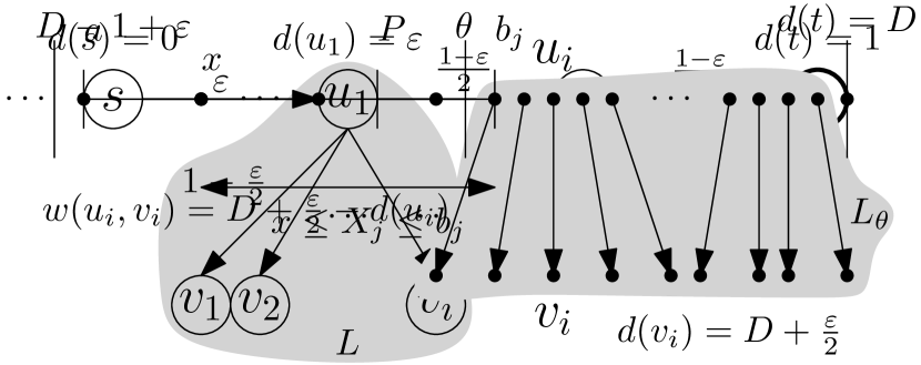
(a) No pruning, even if predictions are perfect ($\varepsilon=0$).

(b) No pruning, even if many relevant edges $(u_{i},v_{i})\in L_{\theta}$.

Figure 1: Instances in which no savings can be expected from our algorithm

4.2 Partial Random Instances

Based on these examples, it is clear that we need to further restrict the power of the adversary. We therefore introduce randomness in the instances to obtain a more fine-grained understanding of the savings achieved by our algorithm. Generally speaking, we will do this by enforcing randomness on some of the edges, while allowing the adversary to still control the rest of the input instance.

The setup is as follows: We suppose that the adversary can fix the set $Q=\{u_{1},\dots,u_{l}\}$ of nodes that are removed from the priority queue, where $u_{i}$ is the node removed in iteration $i$, and the corresponding distances $d(u_{1})\leq\dots\leq d(u_{l})$ of these nodes. Further, the adversary can fix all outgoing edges of the nodes in $Q$. Note that by doing so we implicitly allow that the adversary can fix the weights of certain edges to enforce this configuration (because these weights determine the order in which the nodes are removed from the priority queue). Crucially, however, we do not allow that the adversary can fix the weights of the relevant edges in $L_{\theta}$: the weight of each relevant edge in $L_{\theta}$ is random.

Now, in this partially random setting, the weights for all edges $(u,v)\in L_{\theta}$ are independent and the distance labels $d(u)+w(u,v)$ are uniform on $[D,d(u)+1]$ (Bast et al. (2003)). This is because $(u,v)\in L_{\theta}$ implies $d(u)+w(u,v)\geq D$ and $d(u)+w(u,v)\leq d(u)+1$, but nothing else.

Given this partially random adversarial setting, we can lower bound the probability of pruning an edge in $L_{\theta}$. Like in the previous examples, the adversary still has enough power to setup the instance such that none of these edges are pruned based on the bound $B$. In contrast, each of these edges is pruned with positive probability due to the prediction $P$. For the edges in $L_{\theta}$ we know that the necessary condition for pruning, $d(u)>D+1-\varepsilon$, holds.

Lemma 1.

Suppose $L_{\theta}$ is defined as above, with $\theta=D+\gamma\varepsilon-1$, for some $\gamma\in(1,\frac{1}{\varepsilon}]$. Let $X_{e}$ be a random variable which equals 1 if edge $e\in L_{\theta}$ is pruned and zero otherwise. Then $\mathbf{P}(X_{e}=1)\geq 1-\frac{1}{\gamma}.$

Proof.

Let $e=(u,v)\in L_{\theta}$ be a relevant edge and let $d(v)$ be the distance of $v$ at the end of the algorithm. Then $e$ is pruned whenever the tentative distance $tent:=d(u)+w(u,v)$ exceeds the prediction $P$. As argued before, $e\in L_{\theta}$ implies that $d(u)+w(u,v)$ is uniformly distributed on $[D,d(u)+1]$. Furthermore, note that $1-(D-d(u))\geq\gamma\varepsilon$ follows from $d(u)\geq\theta$ and the definition of $\theta$ and note that $D+\varepsilon$ is contained in the interval $[D,d(u)+1]$, since $D+\varepsilon\leq D+\gamma\varepsilon\leq d(u)+1$. We can simply apply the cumulative distribution function for the uniform distribution:

$$\mathbf{P}(X_{e}=1)=\mathbf{P}(tent\geq P)=\mathbf{P}(d(u)+w(u,v)\geq D+\varepsilon)=\frac{d(u)+1-(D+\varepsilon)}{d(u)+1-D}\geq 1-\frac{1}{\gamma}.$$

∎

We give some intuition for the lemma: The number of edges in $L_{\theta}$ is largest when $\gamma$ is close to 1, and the lemma shows there is a small positive probability for each of those to be pruned by the prediction. As $\gamma$ increases to $\frac{1}{\varepsilon}$, the threshold $\theta$ approaches $D$ and the size of $L_{\theta}$ decreases. So the number of relevant edges decreases, while the probability that each such edge is pruned increases.

Define $X$ as the total number of pruned edges in $L_{\theta}$, i.e., $X=\sum_{e\in L_{\theta}}X_{e}$. theoremprunedEdgesWhp Suppose $L_{\theta}$ is defined as above, with $\theta=D+\gamma\varepsilon-1$, for some $\gamma\in(1,\frac{1}{\varepsilon}]$. Then the expected number of pruned edges in $L_{\theta}$ is $\mathbf{E}[X]\geq(1-\tfrac{1}{\gamma})|L_{\theta}|.$ Further, if $(1-\frac{1}{\gamma})|L_{\theta}|\geq 8\ln n$, then $X\geq\frac{1}{2}(1-\frac{1}{\gamma})|L_{\theta}|$ with high probability, i.e., $\mathbf{P}(X\geq\frac{1}{2}(1-\frac{1}{\gamma})|L_{\theta}|)\geq 1-\frac{1}{n}$.

Proof.

By linearity of expectation, it follows from Lemma 1:

$$\mathbf{E}[X]=\mathbf{E}\left[\sum_{e\in L_{\theta}}X_{e}\right]=\sum_{e\in L_{\theta}}\mathbf{E}[X_{e}]=\sum_{e\in L_{\theta}}\mathbf{P}(X_{e}=1).$$

Note that $X=\sum_{e\in L_{\theta}}X_{e}$ is a sum of $|L_{\theta}|$ independent random variables. Let $\mu:=\mathbf{E}[X]$ be the expected value of $X$. The following (standard) Chernoff bound holds for every $\delta\in(0,1)$:

$$\mathbf{P}(X\leq(1-\delta)\mu)\leq e^{-\mu\delta^{2}/2}.$$

By choosing $\delta=\frac{1}{2}$, we obtain

$$\mathbf{P}\left(X\leq\frac{1}{2}\mu\right)\leq e^{-\mu/8}\leq\frac{1}{n},$$

where the second inequality holds because $\mu=\mathbf{E}[X]\geq(1-\frac{1}{\gamma})|L_{\theta}|\geq 8\ln n$ by our assumption.

Using this, we conclude that

$$\mathbf{P}\left(X\geq\frac{1}{2}\left(1-\frac{1}{\gamma}\right)|L_{\theta}|\right)\geq\mathbf{P}\left(X\geq\frac{1}{2}\mu\right)\geq 1-\frac{1}{n}.$$

∎

4.3 Random model

We consider random instances constructed according to the model introduced in Section 2. For these instances, we show that our Dijkstra-Prediction algorithm saves a significant number of queue operations compared to Dijkstra-Pruning.

In the random model, it is not straightforward to compute the size of $L_{\theta}$. Therefore, we will consider a specific subset of $L_{\theta}$ for which we are able to compute the size. More specifically, we only consider the edges $(u,v)$ from $L_{\theta}$ for which the final distance $d(v)$ is larger than $D$, i.e., edges from $L_{\theta}$ that lead to a node $v$ which is not in $Q$. Note that there could be multiple edges in $L_{\theta}$ that lead to such a node $v\not\in Q$. In that case, we only consider the (unique) edge in $L_{\theta}$ which has led to an insertion of $v$ into the priority queue in the standard Dijkstra algorithm (disregarding edges that have led to a decrease priority operation). We use $L^{\prime}_{\theta}$ to denote this subset of $L_{\theta}$:

$$L^{\prime}_{\theta}:=\{(u,v)\in L_{\theta}\;:\;\text{$(u,v)$ leads to insertion of $v$ in {PQ}\ of {Dijkstra}}\}.$$

In the Dijkstra algorithm, all the end nodes of edges in $L_{\theta}^{\prime}$ are inserted in the priority queue, but they are never removed. Dijkstra-Prediction can actually save a number of these insert operations by pruning the edges in $L_{\theta}^{\prime}$. We will lower bound these savings by computing an upper bound for the number of these nodes which are still inserted in our Dijkstra-Prediction algorithm. Consequently, all the edges which lead to nodes which are not inserted in Dijkstra-Prediction are pruned.

First, we will prove the following Key Lemma which will help us to upper bound the probability of inserting an edge below. Below, we use $[k]$ to denote the set $\{1,\ldots,k\}$.

[Key Lemma]lemmakeyLemma Let $X_{j},j=1,\ldots,k+1$, be $k+1$ uniform random variables, with $X_{j}$ uniform on $[a,b_{j}]$ and $b_{1}\leq\cdots\leq b_{k+1}$. Let $P>0$ be a real number, which is contained in all intervals, i.e., $a<P<b_{1}$. Let $\mathcal{E}_{1}$ be the event $\{X_{k+1}\leq X_{j},\forall j\in[k]\}$ and let $\mathcal{E}_{2}$ be the event $\{X_{k+1}\leq P\}$. Then: $\textstyle\mathbf{P}(\mathcal{E}_{1}\wedge\mathcal{E}_{2})\leq\frac{1}{k+1}(1-(1-\frac{P-a}{b_{k}-a})^{k+1}).$

Proof.

We will upper bound the probability by conditioning on values of $X_{k+1}$, using the law of total probability and applying the density function of $X_{k+1}$: $f_{X_{k+1}}(s)=\frac{1}{b_{k+1}-a}$.

$$\mathbf{P}(\mathcal{E}_{1}\wedge\mathcal{E}_{2}) =\int_{a}^{b_{k+1}}\mathbf{P}(\mathcal{E}_{1}\wedge\mathcal{E}_{2}\;|\;X_{k+1}=x)f_{X_{k+1}}(x)dx$$

$$=\frac{1}{b_{k+1}-a}\int_{a}^{b_{k+1}}\mathbf{P}(\mathcal{E}_{1}\wedge\mathcal{E}_{2}\;|\;X_{k+1}=x)dx$$

Since $\mathbf{P}(\mathcal{E}_{1}\wedge\mathcal{E}_{2}\;|\;X_{k+1}=x)=0$ if $x>P$, we can write:

$$\mathbf{P}(\mathcal{E}_{1}\wedge\mathcal{E}_{2}\;|\;X_{k+1}=x) =\mathbf{P}(\mathcal{E}_{1}\wedge\mathcal{E}_{2}\;|\;\{X_{k+1}=x\}\wedge\{x\leq P\})$$

$$=\mathbf{P}(\{X_{k+1}\leq X_{j},\forall j\}\wedge\{X_{k+1}\leq P\}\;|\;\{X_{k+1}=x\}\wedge\{x\leq P\})$$

$$=\mathbf{P}(x\leq X_{j},j=1,\ldots,k\;|\;\{X_{k+1}=x\}\wedge\{x\leq P\})$$

$$=\mathbf{P}(x\leq X_{j},j=1,\ldots,k\;|\;x\leq P)$$

$$=\prod_{j=1}^{k}\mathbf{P}(x\leq X_{j}\;|\;x\leq P)$$

$$=\prod_{j=1}^{k}\left(1-\frac{x-a}{b_{j}-a}\right)$$

$$\leq\left(1-\frac{x-a}{b_{k}-a}\right)^{k}.$$

The third equality holds because the conditioning already implies that $X_{k+1}\leq P$. The fourth equality holds since the value of $X_{j},j=1,\ldots,k$ is independent of the value of $X_{k+1}$. Thereafter we use that all the $X_{j}$’s are identically distributed, and we use the cumulative distribution function of the uniform distribution. In the last inequality we exploit that $b_{j}-a\leq b_{k}-a$ for all $j$. We can use this, together with $\frac{b_{k}-a}{b_{k+1}-a}\leq 1$, to upper bound the expectation of $\mathcal{E}_{1}\wedge\mathcal{E}_{2}$:

$$\mathbf{P}(\mathcal{E}_{1}\wedge\mathcal{E}_{2}) \leq\frac{1}{b_{k+1}-a}\int_{a}^{P}\left(1-\frac{x-a}{b_{k}-a}\right)^{k}dx$$

$$=\frac{1}{b_{k+1}-a}\left[-\frac{b_{k}-a}{k+1}\left(1-\frac{x-a}{b_{k}-a}\right)^{k+1}\right]_{a}^{P}$$

$$=\frac{1}{b_{k+1}-a}\left[-\frac{b_{k}-a}{k+1}\left(1-\frac{P-a}{b_{k}-a}\right)^{k+1}+\frac{b_{k}-a}{k+1}\right]$$

$$=\frac{b_{k}-a}{b_{k+1}-a}\frac{1}{k+1}\left[1-\left(1-\frac{P-a}{b_{k}-a}\right)^{k+1}\right]$$

$$\leq\frac{1}{k+1}\left[1-\left(1-\frac{P-a}{b_{k}-a}\right)^{k+1}\right].$$

∎

We will continue to lower bound the expected number of end nodes of edges in $L_{\theta}^{\prime}$ which are inserted in the Dijkstra-Prediction algorithm, despite the prunings. We call this quantity $\text{INRP}_{\theta}$. We condition on the event $E_{l}$, which implies not only the adversarial setting introduced in the previous section, but also that the size of $L_{\theta}^{\prime}$ equals $l$.

theoremINRPtheorem Suppose $L_{\theta}^{\prime}$ is defined as above, with $\theta=D+\gamma\varepsilon-1$, for some $\gamma\in(1,\frac{1}{\varepsilon}]$. Let $\text{INRP}_{\theta}$ be the number of end nodes of edges in $L_{\theta}^{\prime}$ which are inserted but never removed in the Dijkstra-Prediction algorithm. Under the conditioning of the event $E_{l}$, i.e., $|L_{\theta}^{\prime}|=l$ and the adversarial setting, we have that: $\textstyle\mathbf{E}[\text{INRP}_{\theta}\;|\;E_{l}]\leq\frac{1}{q}(1+\ln(\frac{lq}{\gamma})).$

Proof.

Let $l$ be the size of $L_{\theta}^{\prime}$ and let $e_{1}=(u_{1},v_{1}),e_{2}=(u_{2},v_{2}),\ldots,e_{l}=(u_{l},v_{l})$ be all the edges in $L_{\theta}^{\prime}$. Note that there might be repetitions in the $u_{i}$’s, but all the $v_{i}$’s are distinct. For $i=1,\ldots,l$, define $X_{i}=d(u_{i})+w(e_{i})$. We observed in the previous section that for all edges $e_{i}$ in $L_{\theta}^{\prime}$ it holds that $X_{i}$ is random uniform on $[D,d(u_{i})+1]$.

In Dijkstra-Pruning  $e_{i}$ leads to an insertion only if $X_{i}$ is smaller than $X_{j}$ for every free $v_{j}$, with $j<i$. Suppose that there are $k$ of these free $v_{j}$’s preceding $v_{i}$ in the endpoints of $L_{\theta}^{\prime}$. In Dijkstra-Prediction, an extra condition must be met, namely that $X_{i}$ does not exceed the prediction. To lower bound the expectation of $\text{INRP}_{\theta}$, we partition over $k$, the number of free $v_{j}$ preceding $v_{i}$:

$$\mathbf{E}[\text{INRP}_{\theta}\;|\;E_{l}]\leq\sum_{1\leq i\leq l}\sum_{0\leq k<i}\binom{i-1}{k}q^{k}(1-q)^{i-1-k}\mathbf{P}(\{X_{i}\leq X_{j},\forall j\in[k]\}\wedge\{X_{i}\leq P\})$$

To be able to apply our Key Lemma (Lemma 4.3), we need that the variables $X_{j}$ must be random uniform. We have already shown that they are random uniform on $[D,d(u_{j})+1]$, for which the upper bounds increase as $j$ increases. Moreover, we need that $P<b_{1}$, which holds since for all edges in $L_{\theta}^{\prime}$ we have $d(u_{i})+1>P$. Therefore, we can apply our Key Lemma to upper bound the probability in the sum above by

$$\textstyle\frac{1}{k+1}\left[1-\left(1-\frac{P-D}{d(u_{k})+1-D}\right)^{k+1}\right]\textstyle\leq\frac{1}{k+1}\left[1-\left(1-\frac{1}{\gamma}\right)^{k+1}\right],$$

which gives

$$\mathbf{E}[\text{INRP}_{\theta}\;|\;E_{l}] \leq\sum_{1\leq i\leq l}\sum_{0\leq k<i}\binom{i-1}{k}q^{k}(1-q)^{i-1-k}\frac{1}{k+1}$$ (2)

$$-\sum_{1\leq i\leq l}\sum_{0\leq k<i}\binom{i-1}{k}q^{k}(1-q)^{i-1-k}\frac{1}{k+1}\left(1-\frac{1}{\gamma}\right)^{k+1}.$$ (3)

We know from Bast et al. (2003) that (2) is equal to $\sum_{1\leq i\leq l}\frac{1}{iq}(1-(1-q)^{i})$. We will use similar techniques to obtain such an expression for (3). As in Bast et al. (2003), we use $\binom{i-1}{k}\frac{1}{k+1}=\frac{1}{i}\binom{i}{k+1}$, and then use the binomium of Newton to rewrite the sum:

$$\eqref{eq:line2}=\sum_{1\leq i\leq l}\frac{1}{iq}\sum_{0\leq k<i}\binom{i}{k+1}\left(q\left(1-\frac{1}{\gamma}\right)\right)^{k+1}(1-q)^{i-(k+1)}$$

$$=\sum_{1\leq i\leq l}\frac{1}{iq}\left[\sum_{0\leq k\leq i}\binom{i}{k}q^{k}\left(1-\frac{1}{\gamma}\right)^{k}(1-q)^{i-k}-(1-q)^{i}\right]=\sum_{1\leq i\leq l}\frac{1}{iq}\left[\left(1-\frac{q}{\gamma}\right)^{i}-(1-q)^{i}\right].$$

Combining these two bounds, we obtain

$$\mathbf{E}[\text{INRP}_{\theta}\;|\;E_{l}] \leq\sum_{1\leq i\leq l}\frac{1}{iq}\left[1-(1-q)^{i}-\left(1-\frac{q}{\gamma}\right)^{i}+(1-q)^{i}\right]=\sum_{1\leq i\leq l}\frac{1}{iq}\left[1-\left(1-\frac{q}{\gamma}\right)^{i}\right].$$

As in Bast et al. (2003), we split the sum at a yet to be determined index $i_{0}$. For $i<i_{0}$, we estimate $(1-(1-\frac{q}{\gamma})^{i})\leq\frac{iq}{\gamma}$, and for $i\geq i_{0}$, we use $(1-(1-\frac{q}{\gamma})^{i})\leq 1$. We obtain:

$$\mathbf{E}[\text{INRP}_{\theta}\;|\;E_{l}] \leq\frac{i_{0}}{\gamma}+\frac{1}{q}\sum_{i_{0}\leq i\leq l}\frac{1}{i}\approx\frac{i_{0}}{\gamma}+\frac{1}{q}\ln\left(\frac{l}{i_{0}}\right)\leq\frac{1}{q}\left(1+\ln\left(\frac{lq}{\gamma}\right)\right),$$

where the last inequality follows by noting that $\frac{i_{0}}{\gamma}+\frac{1}{q}\ln(\frac{l}{i_{0}})$ attains its minimum with respect to $i_{0}$ at $i_{0}=\frac{\gamma}{q}$. ∎

Now, suppose $D$ lies in $[0,1-\varepsilon)$ and let $\gamma$ be $\frac{1-D}{\varepsilon}$, which makes $\theta$ equal to 0. This means that all the edges which lead to nodes that are inserted but not removed by Dijkstra are in the set $L_{\theta}^{\prime}$. Said differently, the size of $|L_{\theta}^{\prime}|$ is equal to the number of nodes that are inserted but never removed in the priority queue by the Dijkstra algorithm. Bast et al. (2003) estimate the expected value of this quantity, conditional on that many nodes are reachable from $s$ (“$R$ is large”). We summarise their findings in the following proposition.

Proposition 1 (Bast et al. (2003)).

Consider an instance from the random model introduced in Section 2. Let $R$ be the number of reachable nodes from $s$ in the random graph. Then if $c\geq 8$ and $f\geq 4\ln(n)$, it holds that $R$ is large, i.e. $R\geq(1-\delta)\alpha n$, for some $\alpha$ such that $\alpha=1-\exp(-c\alpha)$ and $\delta$ small like 0.01. Moreover, the expected number of nodes that are inserted but never removed in the priority queue by the Dijkstra algorithm, given that $R$ is large, is approximately:

$$\mathbf{E}[INRS\;|\;R\text{ is large}]\approx\frac{c-1}{q}.$$

By exploiting this proposition, we can drop the dependency on the size of $L_{\theta}$ and we obtain the following theorem. theoremfinalSavings Suppose $D$ lies in $[0,1-\varepsilon)$. Let INRP be the number of nodes that are inserted but never removed by Dijkstra-Prediction. Then $\textstyle\mathbf{E}[\text{INRP}\;|\;R\text{ is large}\,]\leq\frac{1}{q}\left(1+\ln(c-1)-\ln\left(\frac{1-D}{\varepsilon}\right)\right).$

Proof.

We can upper bound the expected value of $\text{INRP}_{\theta}$ given in Theorem 4.3 as follows: Since $\ln(\frac{lq}{\gamma})$ is a convex function of $l$, we can replace $l$ simply by the expectation of INRS (using Proposition 1). We obtain

$$\textstyle\mathbf{E}[\text{INRP}\;|\;R\text{ is large}\,] \textstyle\leq\frac{1}{q}\left(1+\ln\left(\frac{(c-1)q\varepsilon}{q(1-D)}\right)\right)=\frac{1}{q}\left(1+\ln(c-1)-\ln\left(\frac{1-D}{\varepsilon}\right)\right).$$

∎

Let INRR denote the number of nodes that are inserted but never removed by Dijkstra-Pruning. It is shown in Bast et al. (2003) that $\mathbf{E}[\text{INRR}\;|\;R\text{ is large}\,]\leq\frac{1}{q}\left(1+\ln(c-1)\right).$ That is, compared to the Dijkstra-Pruning algorithm, our Dijkstra-Prediction algorithm saves $\frac{1}{q}\ln(\frac{1-D}{\varepsilon})$ insertions of such nodes. So even though Dijkstra-Pruning already saves a significant number of insertions, Dijkstra-Prediction is able to further improve on this. Naturally, these savings grow whenever the prediction becomes more accurate and $\varepsilon$ decreases.

In our experiments, we consider random instances with $n=1000$, $c=8$ and $q=0.02$. For these instances, $D$ is approximately 0.55. With a prediction $P=D+\varepsilon$ which overestimates $D$ by at most $\varepsilon=0.1$ (which seems reasonable from the experiments), the expected number of INRP of Dijkstra-Prediction is at most 63. In comparison, the expected number of INRS of Dijkstra is 350; so our algorithm saves at least 287 of these insertions. The expected number of INRR of Dijkstra-Pruning is at most 137; our algorithms significantly improves upon this by exploiting the prediction.

5 Prediction Methods

The Prediction algorithm used in our algorithm Dijkstra-Prediction can be obtained in numerous ways. Below, we explain how we obtain a prediction algorithm based on a machine learning approach. We elaborate on two different machine learning models and compare them to a benchmark prediction. Moreover, two alternative prediction methods based on breadth-first search (BFS) are given.

5.1 ML-based Predictions

In order to make a prediction after $i_{0}$ iterations, we need to be able to describe the current optimisation run by means of some characteristic features. One of the challenges here is to come up with features that capture the essence of the current run such that they can be used by the machine learning model to make a good prediction of the shortest path distance. We do this by keeping track of a lower and upper bound on the shortest path distance in each iteration. More precisely, in iteration $i\leq i_{0}$, the distance $d(u)$ of the node $u$ extracted from the priority queue serves as the lower bound $d_{i}$ and the current value of the pruning bound $B$ is used as the upper bound $B_{i}$. The resulting sequence $X=((d_{1},B_{1}),(d_{2},B_{2}),\dots,(d_{i_{0}},B_{i_{0}}))$ of these lower and upper bounds for the first $i_{0}$ iterations then constitutes what we call the trace of the algorithm.

A training sample and target for the machine learning algorithm then consists of the trace $X$ and the corresponding shortest path distance $D$, respectively. The set of samples for the machine learning models can be created by executing a run of Dijkstra-Pruning on each problem instance of the training set. During this run, both the trace $X$ and the final shortest path distance $D$ need to be stored. Before the traces are used to train the machine learning models, we normalise each feature by subtracting the mean and divide by the standard deviation. To prevent blowing up the mean value of the upper bound feature, all bounds $B_{i}$ which are equal to the initial value of $B=\infty$ are set to $0$.

We implemented and compared two standard machine learning models, namely a neural network model and a linear regression model. The neural network model that we use is a straightforward multilayer perceptron network consisting of two hidden layers, for which we optimise the number of nodes per layer by a $k$-fold cross validation (see, e.g., Refaeilzadeh et al. (2009) for more details). To verify whether anything has been learned by these models at all, the results for these models are compared with a straightforward benchmark prediction. This benchmark prediction, which is independent of the instance, is computed by taking the average of the shortest path distance for each instance in the training set.

5.2 BFS-based Predictions

As an alternative to the machine learning models given in Section 5, we implement two prediction methods that are based on breadth-first search (BFS). For each instance, we can simply run a BFS from the source node $s$ to determine a path $P^{\textit{BFS}}$ to any of the target nodes having the smallest number of edges. We also call $P^{\textit{BFS}}$ a BFS-path and use $L^{\textit{BFS}}$ to denote its length (i.e., number of edges). Note that, equivalently, $L^{\textit{BFS}}$ is the shortest path distance to any of the target nodes if all edge weights are set to 1. We use this BFS-path to derive two different predictions of the actual shortest path distance $D$: (i) bfs: We define the prediction $P$ as $L^{\textit{BFS}}\cdot\mu_{w}$, where $\mu_{w}$ is the expected edge weight. (ii) $w$-bfs: We define the prediction $P$ as the sum of the actual weights on $P^{\textit{BFS}}$, i.e., $P=\sum_{e\in P^{\textit{BFS}}}w(e)$. Note that that the latter prediction might overestimate but never underestimate the actual distance $D$.

6 Experimental Findings

In this section, we present our experimental findings. We first introduce our experimental setup and then discuss the results and insights we obtained from the experiments.

6.1 Experimental Setup

We generated 100,000 instances of the SSMTSP problem using the random model described in Section 2 with $n=1000$ nodes, edge probability $p=c/n$ with $c=8$, and target probability $q=f/n$ with $f=20$. The edge weights were chosen independently uniformly at random from $[0,1]$. Further, we fixed the length of the constructed traces to $i_{0}=10$. We only accepted an instance if Dijkstra-Pruning executed more than $i_{0}$ iterations to ensure that Dijkstra-Prediction reaches the point where a prediction is made. This set of 100,000 instances was split into a training set of 80,000 instances used for building the machine learning models, a validation set of 10,000 instances used for parameter tuning and a test set of 10,000 instances used for the final experiments.

To get an idea of a few parameters related to the shortest path distance in the generated instances, we provide some statistical data for the validation and test set in Table 1. We computed the average number of edges on a shortest path, the average, minimum and maximum cost of a shortest path, and the average weight of an edge on a shortest path. Note that the first row refers to these parameters with respect to the actual random weights, while the second row refers to the case when all edge weights are set to $1$.

	edges	mean	min	max	$w$-mean
rand	4.363	0.553	0.065	1.848	0.127
unit	2.225	1.154	0.129	3.217	1.000

Table 1: Statistics on different shortest path parameters for 20,000 instances (validation and test set).

6.2 Machine Learning Results

For each of the 80,000 graphs in the training set, we executed a run of Dijkstra-Pruning, during which we stored both the features $X$ and the final returned shortest path distance $y$. After running this, we had a training set of 80,000 samples, where each sample was of shape $(X,y)$. We used these 80,000 samples to built both a neural network and a linear regression model.

The number of nodes in the two hidden layers of the neural network was optimised by minimising the mean absolute error (MAE) in a $k$-fold cross validation with $k=4$ and a batch size of 256. We tested layer sizes $8,16,32,64$ and $128$; the results for the smoothed validation Mean Absolute Error can be found in Figure 2. We decided to use 16 nodes per layer and train for 47 epochs. We did not use the validation set of 10,000 instances in the $k$-fold cross validation, since it was used to tune parameters $\alpha$ and $\beta$. We also tested a linear regression and the benchmark prediction, but the neural network performed best in both the training and the test set.

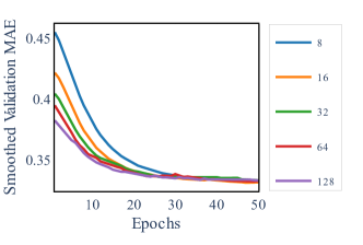
Figure 2: Normalised smoothed mean absolute error of the validation set for different hidden layer sizes.

Algorithm	NN	LR	AB
Train MAE	0.0619	0.0883	0.1469
Train MAPE	0.1228	0.1844	0.3150
Test MAE	0.0617	0.0880	0.1477
Test MAPE	0.1217	0.1837	0.3160

Table 2: Mean absolute error (MAE) and mean absolute percentage error (MAPE) for neural network (NN), linear regression (LR) and averaging benchmark (AB).

The results for the performance of the neural network, linear regression and the benchmark are given in Table 2. Both machine learning models perform better than the benchmark prediction, in both the training and test set. Moreover, the neural network outperforms the linear regression model on both the training and the test set.

6.3 Benchmark Algorithm Oracle

In order to assess the performance of the different algorithms, we decided to use the following (idealised) benchmark algorithm to compare against: We run Dijkstra-Pruning with the pruning bound $B$ being initialised with the actual shortest path distance $D$. We refer to this algorithm as Oracle.

Note that this algorithm only inserts nodes into the priority queue which are necessary for finding the shortest path distance $D$. Said differently, the algorithm spends the minimum possible amount of work to provide a certificate of optimality for the shortest path distance $D$; no other algorithm could spend less work (as long as we insist that the shortest path distance is computed correctly always).

6.4 Parameter Tuning

There are two parameters in the Update-Prediction procedure which decide how to handle the machine learning prediction. The first one is $\alpha$, which specifies the amount by which the initial prediction is inflated. The second one is $\beta$, the amount by which the prediction is inflated. We investigate the impact of these parameters on the queue size; see Figure 3 (bottom layer, both figures for same instance). On the left, we fix $\beta=1.3$ and vary $\alpha$; on the right we fix $\alpha=1.3$ and vary $\beta$. As is visible from these plots, a larger $\alpha$ means that the first call of Update-Prediction occurs later. Also, a larger $\beta$ leads to a larger number of nodes inserted during Update-Prediction.

We tested several configurations for $\alpha$ and $\beta$ on the instances in the validation set. Table 3 and Table 4 state the respective number of queue operations $Q$ and the cumulative queue size $C$ for various choices. As it turns out, for both these performance indicators it is best to choose $\alpha$ and $\beta$ small.

$\alpha\backslash\beta$	1.05	1.10	1.20	1.50	2.00
1.00	153.08	153.59	154.90	158.55	160.20
1.05	154.37	154.80	155.83	158.08	158.84
1.10	156.06	156.37	157.06	158.39	158.74
1.20	160.38	160.50	160.82	161.20	161.30
1.50	172.57	172.58	172.58	172.61	172.61
2.00	182.27	182.27	182.27	182.27	182.27

Table 3: Average number of queue operations ($Q$) for Dijkstra-Prediction for different values of $\alpha$ and $\beta$ on the validation set.

$\alpha\backslash\beta$	1.05	1.10	1.20	1.50	2.00
1.00	2446.0	2561.9	2740.4	3115.7	3274.6
1.05	2573.5	2669.2	2815.5	3067.5	3150.1
1.10	2732.6	2805.3	2914.2	3065.1	3104.4
1.20	3112.6	3148.4	3197.7	3251.9	3266.3
1.50	4104.3	4106.6	4109.5	4114.2	4114.2
2.00	4809.9	4809.9	4809.9	4809.9	4809.9

Table 4: Average cumulative queue size ($C$) for Dijkstra-Prediction for different values of $\alpha$ and $\beta$ on the validation set.

6.5 Discussion of Results

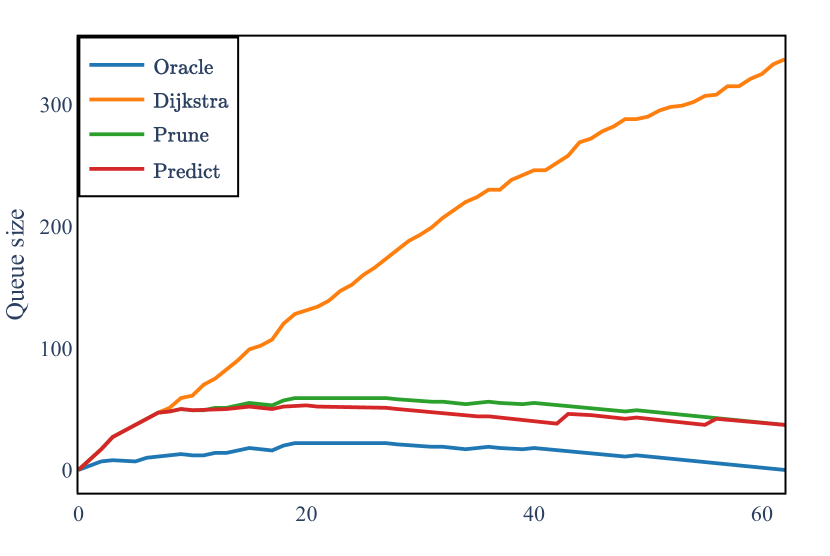
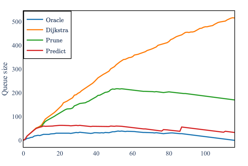
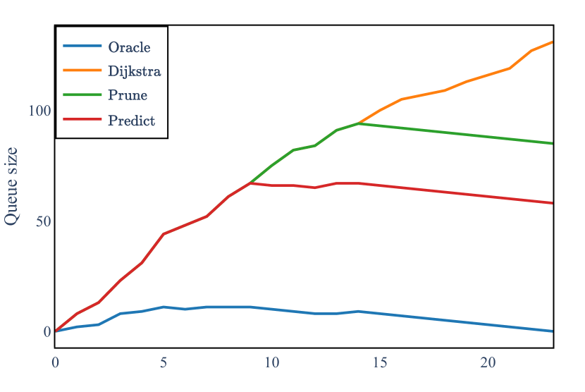
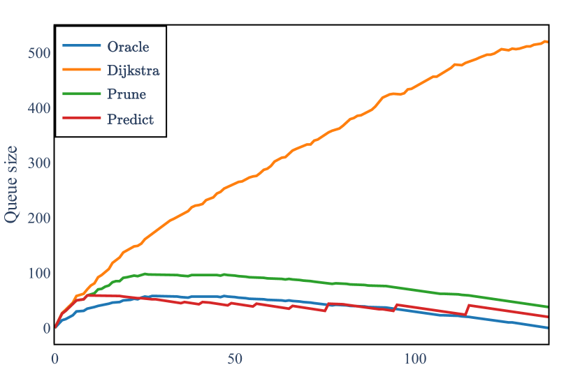
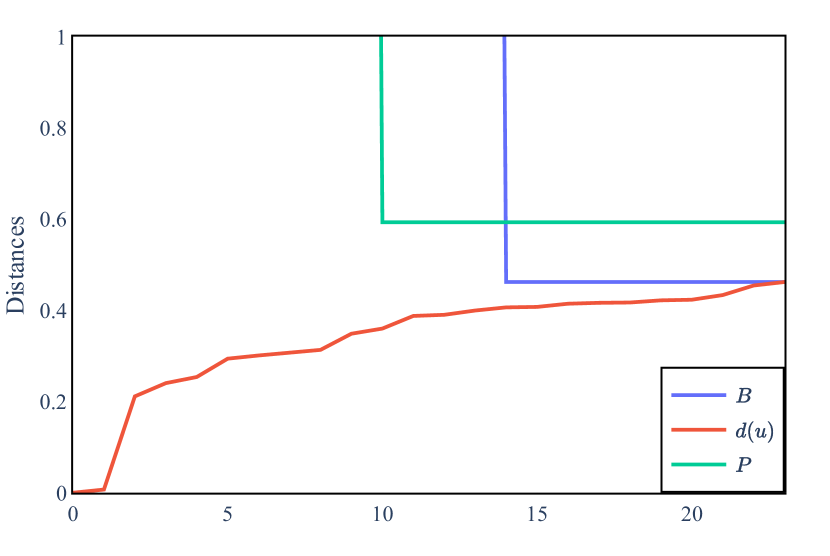
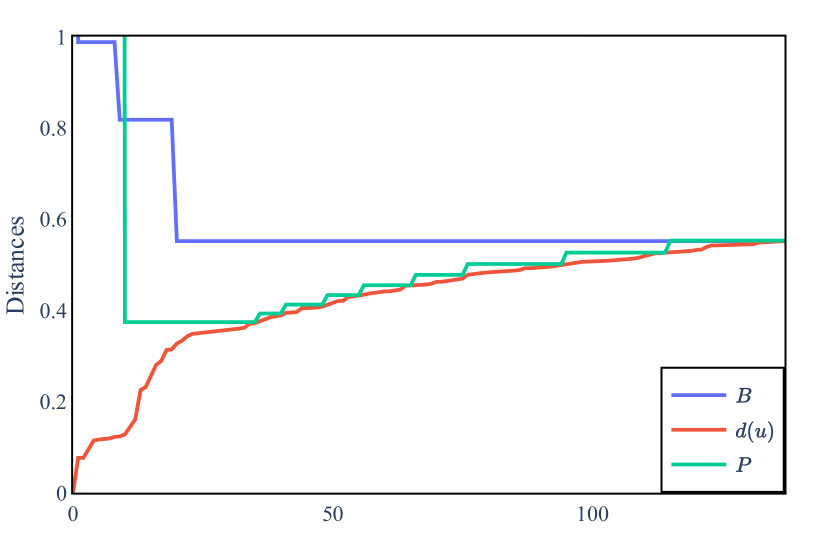
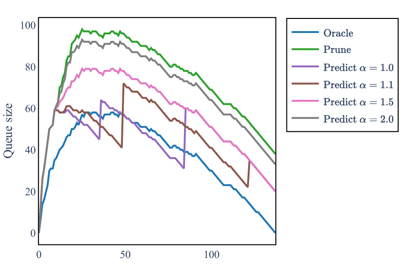
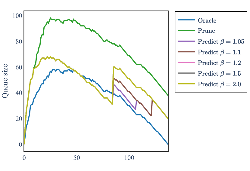
Figure 3: (In all plots the $x$-axis refers to the number of iterations.) Top two layers (four distinctive instances): queue size of the algorithms. Third layer (same instances as in layer two): distance $d(u)$ together with $B$ and $P$ for the Dijkstra-Prediction. Bottom layer: queue size for fixed $\beta=1.3$ and varying $\alpha$ (left) and fixed $\alpha=1.3$ and varying $\beta$ (right) for Dijkstra-Prediction.

We start by considering how the queue sizes differ for the different algorithms; see Figure 3 top 2 rows. As to be expected, the queue size of Dijkstra-Prediction never exceeds the one of Dijkstra-Pruning and is larger or close to the one Oracle. The improvement of our Dijkstra-Prediction with respect to Dijkstra-Pruning varies and depends on the instance. Next, we comment on the Update-Prediction procedure; see Figure 3 third row. On the left, no restart was necessary since the prediction was not an overestimation of $D$. This plot also indicates the interplay of the prediction $P$ and the pruning bound $B$; first the former and later the latter providing the smaller upper bound. On the right, we needed to do several Update-Prediction because the initial prediction turned out to be too small. Update-Prediction adds some nodes from the reserve list to the priority queue (queue size increases) and continues. After several inflations of the prediction with $\beta$, the prediction was sufficiently high to find the shortest path distance.

If we zoom in to obtain a more fine-grained picture of the different queue operations executed by the algorithms, the results are as specified in Table 5 (test set). The respective rows state the number of Remove-Min (RM), Insert (IS) and Decrease-Prio (DP) operations, the total number of queue operations ($Q$), the number of trials ($T$), the cumulative queue size $C$ (over all iterations), and the cumulative queue size relative to the Oracle $\bar{C}$. As to be expected, Oracle inserts and removes the minimum possible number of nodes only. As can also be inferred from Invariant 3.2, Dijkstra, Dijkstra-Pruning and Dijkstra-Prediction have the same number of Remove-Min operations.

Observe that the results show that our algorithm Dijkstra-Prediction outperforms all other algorithms, both in terms of the total number of queue operations and cumulative queue size. Dijkstra-Prediction outperforms Dijkstra-Pruning mostly on the number of insertions, as expected from the analysis in Section 4. In terms of cumulative queue size, our algorithm Dijkstra-Prediction even comes close to the benchmark Oracle, the average cumulative queue size being only 1.7 times larger then the one of Oracle; Dijkstra-Pruning perform much worse, being off by a factor $3.6$.

	Oracle	Dijks	Prune	Prediction	bfs	$w$-bfs
RM	59.39	59.39	59.39	59.39	59.39	59.39
IS	59.39	335.50	122.91	91.73	117.66	118.86
DP	0.78	43.96	5.87	2.89	5.29	5.46
$Q$	119.55	438.85	188.17	154.01	182.33	183.70
$T$	1.00	1.00	1.00	2.28	1.23	1.00
$C$	1456.16	13949.37	5245.96	2476.35	4825.09	4980.69
$\bar{C}$	1.00	9.58	3.60	1.70	3.31	3.42

Table 5: Number of Remove-Min (RM), Insert (IS) and Decrease-Prio (DP) operations, the total number of queue operations ($Q$), the number of trials ($T$), the cumulative queue size $C$ (over all iterations), and the cumulative queue size relative to the Oracle $\bar{C}$ for Dijkstra, Dijkstra-Pruning, Dijkstra-Prediction and the oracle algorithm. Averaged over all graphs in the test set.

6.6 Results for Different Graph Parameters

In all results so far, we used a fixed set of parameters for the random graph model, namely an average degree $c$ of 8, and a target probability $q$ of 0.02. A natural question which might arise is how our algorithm performs on a less specific random graph structure. To answer this question, we built a new ML model, which is based on graphs with various random graph parameters, opposed to the single setting it was based on before. This new ML model showed us that, even though this new model is based on graphs with various input parameters, Dijkstra-Prediction is still able to reduce the cumulative queue size.

By taking $c$ from $\{2,5,8,16,32\}$ and $q$ from $\{0.02,0.06,0.18\}$, we created 15 pairs of random graph parameters. For each of these pairs, we constructed 80.000 graphs, which together formed a large training set of 1.2 million instances. We created a machine learning prediction model based on this training set, as explained before in Section 6.2.

For each of the pairs of random graph parameters, we performed the Oracle, Dijkstra, Dijkstra-Pruning and Dijkstra-Prediction algorithm and compared the cumulative queue size of each algorithm to that of the Oracle. Table 6 shows the average relative cumulative queue size of a thousand instances. These results show us two things. Firstly and crucially, for each pair of random graph parameters, Dijkstra-Prediction is able to reduce the cumulative queue size compared to Dijkstra-Pruning. This means that our algorithm does not lose its power to decrease the cumulative queue size, even when it is used on less specific random graph structures. For lower values of $q$, which means there are less target nodes in the instances, Dijkstra-Prediction has a larger improvement over Dijkstra-Pruning than for larger values of $q$. A second and minor thing which these results show us is that the relative cumulative queue size can be lower than 1.0. E.g. when $c=2$ and $q=0.02$, Dijkstra-Prediction has a lower cumulative queue size than Oracle. This seems unexpected, but can be explained by the average number of Update-Prediction routines done for those graph settings, which is 4.83. This fairly large number of Update-Prediction routines shows that the prediction was significantly too low and had to be increased several times. The low prediction caused the queue size to be low as well, which explains the small $\bar{C}$.

	$q=0.02$			0.06			0.18
	Dijkstra	Pruning	Predict	Dijkstra	Pruning	Predict	Dijkstra	Pruning	Predict
$c=2$	2.20	1.57	0.40	2.55	1.61	0.90	2.84	1.66	1.49
5	6.10	2.62	1.01	7.71	2.92	2.19	8.86	2.95	2.82
8	9.58	3.60	1.82	12.97	4.13	3.35	15.02	3.64	3.50
16	16.04	4.76	2.84	24.78	5.26	4.51	31.20	5.07	4.92
32	22.55	6.05	4.15	43.21	6.76	5.95	57.54	6.03	5.89

Table 6: Cumulative queue sizes ($\bar{C}$) relative to the the cumulative queue size of Oracle for Dijkstra, Dijkstra-Pruning and Dijkstra-Prediction algorithm, for different random graph parameters $c$ and $q$.

6.7 Timing results

Next to fine grained results counting operations on random graphs, we also tested the speed of our algorithm. We did this on certain graph instances which amplify the benefit of our algorithm. We call those instances the fortunate instances, which we define in more detail below. Furthermore, we assumed that we had a perfect prediction in our pruning algorithm ($P=D$ and $\alpha=0$), and assumed this prediction was available from the start ($i_{0}=0$).

A fortunate graph instance is defined as follows (see Figure 4 for an example). Two input parameters must be given: the number of nodes, $n\in\mathbb{N}$, and the fraction of nodes which is on the shortest path, $r\in\mathbb{R}_{+}$. From these parameters, the number of nodes on the shortest path, $x$, can be derived: $x:=\lfloor r\cdot n\rfloor$. We denote these nodes on the shortest path as $u_{i}$, for $i=0,\ldots,x-1$. Furthermore, we label $u_{0}$ as the start $s$ and label $u_{x-1}$ as the target $t$. The rest of the $n-x$ nodes in the graph are denoted by $v_{j}$, for $j=1,2,\ldots,n-x$. Next to these $n$ nodes, there are $(x-1)(1+n-x)$ edges in the fortunate graph. There is an edge $(u_{i},u_{i+1})$ for $i=0,1,\dots,x-2$, each with weight $\frac{1}{x-1}$. Together, these edges form the shortest path from $s$ to $t$, counting up to a shortest path length of exactly 1. Furthermore, there are edges $(u_{i},v_{j})$ for $i=0,1,\ldots,x-2$ and $j=1,2,\dots,n-x$. Each edge from $u_{i}$ to $v_{j}$ has length $2-\frac{2i}{x-1}$.

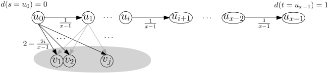
Figure 4: Fortunate instances used for timing analysis. Input parameters: the number of nodes $n\in\mathbb{N}$ and the fraction of nodes which is on the shortest path: $r\in\mathbb{R}_{+}$. The number of nodes on the shortest path, $x\in\mathbb{N}$ can be derived from $n$ and $r$ as follows $x:=\lfloor r\cdot n\rfloor$.

For $i=0,1,\ldots,x-2$ and $j=1,2,\dots,n-x$, we define $P_{ij}$ to be the path going through the first $i+1$ nodes on the shortest path, after which it goes to $v_{j}$, i.e. $P_{ij}=(u_{0},u_{1},\ldots,u_{i},v_{j})$. Then the total length of $P_{ij}$ is as follows:

$$w(P_{ij})=i\cdot\frac{1}{x-1}+2-\frac{2i}{x-1}=2-\frac{i}{x-1}.$$

This means that for a certain node $v_{j}$, the sequence of $w(P_{ij})$’s decreases as $i$ increases, but the path lengths never drop below the shortest path distance which equals 1. Since these $w(P_{ij})$’s strictly decrease, the tentative distance to $v_{j}$ will be updated in each iteration. In the pruning algorithm, this will result in a Decrease-Prio operation in the priority queue. In the Pruning algorithm, this will result in a update of the tentative distance for a node in the reserve set.

	Oracle		Dijkstra		Pruning		orpr
	time	count	time	count	time	count	time	count
RM	0	1250	0	1250	0	1250	0.01	1250
IS	0	1250	0.01	5000	0	5000	0	1250
DP	0	0	2.88	4680000	2.93	4676250	0	0
RRM	-	-	-	-	-	-	0	0
RIS	-	-	-	-	-	-	0.01	3750
RDP	-	-	-	-	-	-	2.22	4676250

Table 7: Number of, and time span of, Remove-Min (RM), Insert (IS) and Decrease-Prio (DP) operations for the priority queue and deletions (RRM), insertions (RIS) and distance updates (RDP) for the reserve set. For a fortunate graph instance with $n=5000$ and $r=0.250$. For the Prediction algorithm, we assumed a perfect prediction which is known from the start: $P=D$, $\alpha=1$ and $i_{0}=0$. A binomial heap structure was used for the priority queues in all four algorithms.

We counted and timed the operations for the Oracle, Dijkstra, Pruning and Prediction algorithm for a fortunate graph instance with $n=5000$ and $r=0.25$, for which the results are shown in 7. As expected due to the construction of the graph, there are many decrease priority operations, which take up most of the time. In the Predict algorithm, these nodes are never inserted into the priority queue, but remain in the reserve set. Therefore, there are many distance updates in the reserve set (exactly as many as DP operations in for Pruning). Crucially however, these distance updates take less time, which makes the Predict algorithm more efficient.

We executed this test for multiple values of $r$ and for two different heap structures, binomial heap and fibonacci heaps. The run time can be seen in Table 8. Especially for the binomial heap and for large $r$, the benefit of our algorithm becomes clearly visible. For the binomial heap structure and the graph instance in which $r=0.35$, the Predict algorithm is 35% faster than the fastest algorithm without prediction (Dijkstra).

		$r=$0.05	0.1	0.25	0.35
binomial	Oracle:	0	0.01	0	0.01
	Dijkstra:	1.41	2.73	5.5	6.54
	Pruning:	1.18	3.09	5.4	7.52
	Predict:	1.3	2.28	4.2	4.82
fibonacci	Oracle:	0.01	0	0.01	0.02
	Dijkstra:	1.06	1.74	3.79	4.67
	Pruning:	1.08	1.85	4.31	4.78
	Predict:	1.03	2.04	4.49	5.08

Table 8: Time for different fortunate graph instances with $n=5000$ and varying fraction of nodes on the shortest path $r$. Two different heap structures where used for the priority queues in the different algorithms.

References

- Bagheri et al. (2008) A. Bagheri, M. R. Akbarzadeh Totonchi, et al. Finding shortest path with learning algorithms. International Journal of Artificial Intelligence, 1, 2008.
- Bast et al. (2003) H. Bast, K. Mehlhorn, G. Schäfer, and H. Tamaki. A heuristic for Dijkstra’s algorithm with many targets and its use in weighted matching algorithms. Algorithmica, 36(1):75–88, 2003.
- Bauer and Delling (2010) R. Bauer and D. Delling. Sharc: Fast and robust unidirectional routing. Journal of Experimental Algorithmics (JEA), 14:2–4, 2010.
- Bengio et al. (2020) Y. Bengio, A. Lodi, and A. Prouvost. Machine learning for combinatorial optimization: a methodological tour d’horizon. European Journal of Operational Research, 2020.
- Chen et al. (2022) J. Chen, S. Silwal, A. Vakilian, and F. Zhang. Faster fundamental graph algorithms via learned predictions. In K. Chaudhuri, S. Jegelka, L. Song, C. Szepesvari, G. Niu, and S. Sabato, editors, Proceedings of the 39th International Conference on Machine Learning, volume 162 of Proceedings of Machine Learning Research, pages 3583–3602. PMLR, 17–23 Jul 2022. URL https://proceedings.mlr.press/v162/chen22v.html.
- Chugh et al. (2021) G. Chugh, S. Kumar, and N. Singh. Survey on machine learning and deep learning applications in breast cancer diagnosis. Cognitive Computation, pages 1–20, 2021.
- Cormen et al. (2009) T. H. Cormen, C. E. Leiserson, R. L. Rivest, and C. Stein. Introduction to algorithms. MIT press, 2009.
- Dijkstra (1959) E. W. Dijkstra. A note on two problems in connexion with graphs. Numerische mathematik, 1(1):269–271, 1959.
- Dinitz et al. (2021) M. Dinitz, S. Im, T. Lavastida, B. Moseley, and S. Vassilvitskii. Faster matchings via learned duals. In M. Ranzato, A. Beygelzimer, Y. Dauphin, P. Liang, and J. W. Vaughan, editors, Advances in Neural Information Processing Systems, volume 34, pages 10393–10406. Curran Associates, Inc., 2021. URL https://proceedings.neurips.cc/paper/2021/file/5616060fb8ae85d93f334e7267307664-Paper.pdf.
- Driscoll et al. (1988) J. R. Driscoll, H. N. Gabow, R. Shrairman, and R. E. Tarjan. Relaxed heaps: An alternative to fibonacci heaps with applications to parallel computation. Communications of the ACM, 31(11):1343–1354, 1988.
- Eden et al. (2022) T. Eden, P. Indyk, and H. Xu. Embeddings and labeling schemes for a. In 13th Innovations in Theoretical Computer Science Conference (ITCS 2022). Schloss Dagstuhl-Leibniz-Zentrum für Informatik, 2022.
- Elkin and Peleg (2004) M. Elkin and D. Peleg. (1+epsilon,)-spanner constructions for general graphs. SIAM Journal on Computing, 33(3):608–631, 2004.
- Fakcharoenphol and Rao (2006) J. Fakcharoenphol and S. Rao. Planar graphs, negative weight edges, shortest paths, and near linear time. Journal of Computer and System Sciences, 72(5):868–889, 2006.
- Fredman and Tarjan (1987) M. L. Fredman and R. E. Tarjan. Fibonacci heaps and their uses in improved network optimization algorithms. Journal of the ACM (JACM), 34(3):596–615, 1987.
- Fredman and Willard (1990a) M. L. Fredman and D. E. Willard. Blasting through the information theoretic barrier with fusion trees. In Proceedings of the twenty-second annual ACM symposium on Theory of Computing, pages 1–7, 1990a.
- Fredman and Willard (1990b) M. L. Fredman and D. E. Willard. Trans-dichotomous algorithms for minimum spanning trees and shortest paths. In Proceedings [1990] 31st Annual Symposium on Foundations of Computer Science, pages 719–725. IEEE, 1990b.
- Fredman and Willard (1993) M. L. Fredman and D. E. Willard. Surpassing the information theoretic bound with fusion trees. Journal of computer and system sciences, 47(3):424–436, 1993.
- Gavoille et al. (2004) C. Gavoille, D. Peleg, S. Pérennes, and R. Raz. Distance labeling in graphs. Journal of Algorithms, 53(1):85–112, 2004.
- Geisberger et al. (2008) R. Geisberger, P. Sanders, D. Schultes, and D. Delling. Contraction hierarchies: Faster and simpler hierarchical routing in road networks. In Experimental Algorithms: 7th International Workshop, WEA 2008 Provincetown, MA, USA, May 30-June 1, 2008 Proceedings 7, pages 319–333. Springer, 2008.
- Geisberger et al. (2012) R. Geisberger, P. Sanders, D. Schultes, and C. Vetter. Exact routing in large road networks using contraction hierarchies. Transportation Science, 46(3):388–404, 2012.
- Gilbert (1959) E. N. Gilbert. Random graphs. The Annals of Mathematical Statistics, 30(4):1141–1144, 1959.
- Gkatzelis et al. (2022) V. Gkatzelis, K. Kollias, A. Sgouritsa, and X. Tan. Improved price of anarchy via predictions. In Proceedings of the 23rd ACM Conference on Economics and Computation, EC ’22, page 529?557, New York, NY, USA, 2022. Association for Computing Machinery. ISBN 9781450391504. doi: 10.1145/3490486.3538296. URL https://doi.org/10.1145/3490486.3538296.
- Goldberg and Werneck (2005) A. V. Goldberg and R. F. F. Werneck. Computing point-to-point shortest paths from external memory. In ALENEX/ANALCO, pages 26–40, 2005.
- Gutman (2004) R. J. Gutman. Reach-based routing: A new approach to shortest path algorithms optimized for road networks. ALENEX/ANALC, 4:100–111, 2004.
- Hagerup (2000) T. Hagerup. Improved shortest paths on the word ram. In Automata, Languages and Programming: 27th International Colloquium, ICALP 2000 Geneva, Switzerland, July 9–15, 2000 Proceedings 27, pages 61–72. Springer, 2000.
- Han (2001) Y. Han. Improved fast integer sorting in linear space. Information and Computation, 170(1):81–94, 2001.
- Hilger et al. (2009) M. Hilger, E. Köhler, R. H. Möhring, and H. Schilling. Fast point-to-point shortest path computations with arc-flags. The Shortest Path Problem: Ninth DIMACS Implementation Challenge, 74:41–72, 2009.
- ich Lauther (2006) U. ich Lauther. An extremely fast, exact algorithm for finding shor test paths in static networks with geographical background. 2006.
- Köhler et al. (2005) E. Köhler, R. H. Möhring, and H. Schilling. Acceleration of shortest path and constrained shortest path computation. In Experimental and Efficient Algorithms: 4th International Workshop, WEA 2005, Santorini Island, Greece, May 10-13, 2005. Proceedings 4, pages 126–138. Springer, 2005.
- Kumar et al. (2018) R. Kumar, M. Purohit, and Z. Svitkina. Improving online algorithms via ml predictions. In Proceedings of the 32nd International Conference on Neural Information Processing Systems, NIPS’18, page 9684?9693, Red Hook, NY, USA, 2018. Curran Associates Inc.
- Lattanzi et al. (2020) S. Lattanzi, T. Lavastida, B. Moseley, and S. Vassilvitskii. Online scheduling via learned weights. In Proceedings of the Fourteenth Annual ACM-SIAM Symposium on Discrete Algorithms, pages 1859–1877. SIAM, 2020.
- Lu and Weng (2007) D. Lu and Q. Weng. A survey of image classification methods and techniques for improving classification performance. International journal of Remote sensing, 28(5):823–870, 2007.
- Lykouris and Vassilvitskii (2021) T. Lykouris and S. Vassilvitskii. Competitive caching with machine learned advice. J. ACM, 68(4), jul 2021. ISSN 0004-5411. doi: 10.1145/3447579. URL https://doi.org/10.1145/3447579.
- Madkour et al. (2017) A. Madkour, W. G. Aref, F. U. Rehman, M. A. Rahman, and S. Basalamah. A survey of shortest-path algorithms. arXiv preprint arXiv:1705.02044, 2017.
- Maue et al. (2010) J. Maue, P. Sanders, and D. Matijevic. Goal-directed shortest-path queries using precomputed cluster distances. Journal of Experimental Algorithmics (JEA), 14:3–2, 2010.
- Medina and Vassilvitskii (2017) A. M. Medina and S. Vassilvitskii. Revenue optimization with approximate bid predictions. In Proceedings of the 31st International Conference on Neural Information Processing Systems, NIPS’17, pages 1856–1864, Red Hook, NY, USA, 2017. Curran Associates Inc. ISBN 9781510860964.
- Mitzenmacher and Vassilvitskii (2020) M. Mitzenmacher and S. Vassilvitskii. Algorithms with predictions. CoRR, abs/2006.09123, 2020. URL https://arxiv.org/abs/2006.09123.
- Möhring et al. (2007) R. H. Möhring, H. Schilling, B. Schütz, D. Wagner, and T. Willhalm. Partitioning graphs to speedup dijkstra’s algorithm. Journal of Experimental Algorithmics (JEA), 11:2–8, 2007.
- Otter et al. (2020) D. W. Otter, J. R. Medina, and J. K. Kalita. A survey of the usages of deep learning for natural language processing. IEEE Transactions on Neural Networks and Learning Systems, 32(2):604–624, 2020.
- Papadimitriou and Steiglitz (1998) C. H. Papadimitriou and K. Steiglitz. Combinatorial Optimization : Algorithms and Complexity. Dover Publications, July 1998. ISBN 0486402584.
- Qayyum et al. (2020) A. Qayyum, J. Qadir, M. Bilal, and A. Al-Fuqaha. Secure and robust machine learning for healthcare: A survey. IEEE Reviews in Biomedical Engineering, 14:156–180, 2020.
- Refaeilzadeh et al. (2009) P. Refaeilzadeh, L. Tang, and H. Liu. Cross-Validation, pages 532–538. Springer US, Boston, MA, 2009. ISBN 978-0-387-39940-9. URL https://doi.org/10.1007/978-0-387-39940-9_565.
- Rizi et al. (2018) F. S. Rizi, J. Schloetterer, and M. Granitzer. Shortest path distance approximation using deep learning techniques. 2018 IEEE/ACM International Conference on Advances in Social Networks Analysis and Mining (ASONAM), Aug 2018. doi: 10.1109/asonam.2018.8508763. URL http://dx.doi.org/10.1109/ASONAM.2018.8508763.
- Sanders and Schultes (2005) P. Sanders and D. Schultes. Highway hierarchies hasten exact shortest path queries. In ESA, volume 3669, pages 568–579. Springer, 2005.
- Sanders and Schultes (2006) P. Sanders and D. Schultes. Engineering highway hierarchies. In ESA, volume 6, pages 804–816. Springer, 2006.
- Schulz et al. (2000) F. Schulz, D. Wagner, and K. Weihe. Dijkstra’s algorithm on-line: An empirical case study from public railroad transport. Journal of Experimental Algorithmics (JEA), 5:12–es, 2000.
- Silver et al. (2017) D. Silver, J. Schrittwieser, K. Simonyan, I. Antonoglou, A. Huang, A. Guez, T. Hubert, L. Baker, M. Lai, A. Bolton, et al. Mastering the game of go without human knowledge. nature, 550(7676):354–359, 2017.
- Silver et al. (2018) D. Silver, T. Hubert, J. Schrittwieser, I. Antonoglou, M. Lai, A. Guez, M. Lanctot, L. Sifre, D. Kumaran, T. Graepel, et al. A general reinforcement learning algorithm that masters chess, shogi, and go through self-play. Science, 362(6419):1140–1144, 2018.
- Sommer (2014) C. Sommer. Shortest-path queries in static networks. ACM Computing Surveys (CSUR), 46(4):1–31, 2014.
- Thorup (1999) M. Thorup. Undirected single-source shortest paths with positive integer weights in linear time. Journal of the ACM (JACM), 46(3):362–394, 1999.
- Thorup and Zwick (2005) M. Thorup and U. Zwick. Approximate distance oracles. Journal of the ACM (JACM), 52(1):1–24, 2005.
- van Emde Boas (1975) P. van Emde Boas. Preserving order in a forest in less than logarithmic time. In 16th Annual Symposium on Foundations of Computer Science (sfcs 1975), pages 75–84. IEEE, 1975.
- Xu and Lu (2022) C. Xu and P. Lu. Mechanism design with predictions. In L. D. Raedt, editor, Proceedings of the Thirty-First International Joint Conference on Artificial Intelligence, IJCAI-22, pages 571–577. International Joint Conferences on Artificial Intelligence Organization, 7 2022. doi: 10.24963/ijcai.2022/81. URL https://doi.org/10.24963/ijcai.2022/81. Main Track.
- Zhao et al. (2010) X. Zhao, A. Sala, C. Wilson, H. Zheng, and B. Y. Zhao. Orion: shortest path estimation for large social graphs. networks, 1:5, 2010.
- Zhao et al. (2011) X. Zhao, A. Sala, H. Zheng, and B. Y. Zhao. Efficient shortest paths on massive social graphs. In 7th International Conference on Collaborative Computing: Networking, Applications and Worksharing (CollaborateCom), pages 77–86. IEEE, 2011.