Stability analysis of an eight parameter SIR-type model including loss of immunity, and disease and vaccination fatalities

Abstract

We revisit here a landmark five parameter SIR-type model of (DvdD, 93, Sec. 4), which is maybe the simplest example where a complete picture of all cases, including non-trivial bistability behavior, may be obtained using simple tools. We also generalize it by adding essential vaccination and vaccination induced death parameters, with the aim of revealing the role of vaccination and its possible failure. The main result is Theorem 5, which describes the stability behavior of our model in all possible cases.

1 Introduction

Motivation. This paper has the dual purpose of providing a short guide to students of deterministic mathematical epidemiology, among which we count ourselves, and at the same time to illustrate the technical work one is faced with in an elementary, but not simple “exercise”. Of course, one can easily find at least five must-read excellent textbooks and thesis surveying this field (with different emphasis: epidemiological, stability, or control), see for example AAM (92); ST (11); Mar (15); Thi (18); BCCF (19); Mon (20); Bac (21); DM (21), and also at least a hundred major papers which are a must read. We hope however that our little guide may help future students decide as to the order in which these materials must be assimilated.

A bit of history. Deterministic mathematical modelling of diseases started with works of Ross on malaria, and imposed itself after the work of KM (27) on the Bombay plague of 1905–06. This was subsequently followed by works on measles, smallpox,chickenpox, mumps, typhoid fever and diphtheria, see for example  Ear (08), and recently the COVID-19 pandemic (see for example   Sch (20); Bac (20); Ket (20); CELT (20); DDMC⁺ (20); SRE⁺ (20); AAL (20); HKT (20); DLKM (20); Fra (20); Bak (20); CGF⁺ (20, 21), to cite just a few representatives of a huge literature). Note that at its beginning, mathematical epidemiology was a collection of similar examples dealing with current epidemics, and no one bothered to define precisely what is an epidemic, mathematically. One answer to this question, reviewed in Appendix B, may be found in the recent paper KS (08).

The deterministic mathematical epidemiology literature may be divided into three streams.

1. “Constant total population” models are the easiest to study. However,  since death is an essential factor of epidemics, the assumption of constant total population (clearly a short term or very large population approximation) deserves some comment. One possible rigorous justification for deterministic constant population epidemiological models comes from slow-fast analysis KK (02); JKKPS (21); Gin (21). This is best understood for models with demography (birth, death), which happen typically on a slower scale than the infectious phenomena. Here there is a natural partition of the compartments into a vector $\vec{\;}\mathsf{i}(t)\in\mathbb{R}_{+}^{-}$ of disease/infectious compartments (asymptomatic, infectious hospitalized,etc). These interact (quickly) with the other input classes like the susceptibles and output classes like the recovered and dead.

   For constant total population” models the total population $N$ clearly plays no role, and one may use the assumption that the rate of infection is independent of $N$, of the form $\beta S(t)I(t)$ (which was called pseudo, or simple mass-action incidence dJDH (95)). Note that this simplification of the rate of infection (adopted in the majority of the literature) is inappropriate for varying population models.

2. Models with constant birth rate (in the analog stochastic model, this would correspond to emigration). These models include the previous class, and preserve some of its nice features, like the uniqueness of the endemic fixed point. They typically satisfy the “${\mathcal{R}}_{0}$ alternative”, established via the next generation matrix approach, and also the fact that the endemic point exists only when ${\mathcal{R}}_{0}>1$ – see DlSNAQI (19) for a recent nice review of several stability results for this class of models.

3. Finally, we arrive to the class our paper is concerned with: models with linear birth-rate $\Lambda N$ ( or constant birth-rate per capita in the analog stochastic model), varying total population $N$, and “proportionate mixing” rate of infection

   $$\beta S(t)\frac{I(t)}{N(t)}.$$

   As far as we know, this stream of literature was initiated in BvdD (90, 93), and allows the possibility of bi-stability when ${\mathcal{R}}_{0}<1$ (absent from the previous models), even in a SIR example with five parameters DvdD (93). .

   This last stream of literature is quite important, since constant birth-rate per capita is a natural assumption.

Despite further remarkable works on particular examples – see for example Gre (97); LGWK (99); Raz (01); LM (02); SH (10); YSA (10); LL (18) (which preferred all direct stability analyses to the next generation matrix approach), the literature on models with varying total population, unlike the two preceding streams, has not yet reached general results.

To understand this failure, it seemed to us a good idea to revisit an important SIR model with disease-induced deaths and loss of immunity DvdD (93); Raz (01). These important works illustrate already some of the complexities which may arise for varying population models, in particular the possibility of bi-stability when ${\mathcal{R}}_{0}<1$. This surprising fact lead us to introduce the concept of strong global stability of the DFE (disease free equilibrium), and to find conditions for this to hold in our example, (see Proposition 4). Since the method used is simply linear programming, we hope to extend this in future work.

Our model. We further added to the extension of KM (27) introduced in  DvdD (93); Raz (01) vaccinations. Grouping together the recovered and vaccinated, our “SIR/V+S” model is described by:

$$S^{\prime}(t) =\Lambda N(t)-\frac{\beta}{N(t)}S(t)I(t)-(\gamma_{s}+\mu)S(t)+\gamma_{r}R(t),$$

$$I^{\prime}(t) =I(t)\left(\frac{\beta}{N(t)}S(t)+\frac{\beta_{r}}{N(t)}R(t)-\gamma-\mu-\nu_{i}\right),$$

$$R^{\prime}(t) =\gamma_{s}S(t)+\gamma I(t)-(\gamma_{r}+\mu+\nu_{r})R(t)-\frac{\beta_{r}}{N(t)}R(t)I(t),$$

$$D^{\prime}(t) =\mu(S(t)+I(t)+R(t)),$$

$$D_{e}^{\prime}(t) =\nu_{i}I(t)+\nu_{r}R(t),$$

$$N^{\prime}(t) =(S(t)+I(t)+R(t))^{\prime}=(\Lambda-\mu)N(t)-\nu_{i}I(t)-\nu_{r}R(t),$$ (1.1)

It involves six states: $S:\mathbb{R}_{\geq 0}\rightarrow\mathbb{N}_{>0}$ describing the number of susceptible individuals in the population, $I:\mathbb{R}_{\geq 0}\rightarrow\mathbb{N}_{>0}$ describing the number of infections, $R:\mathbb{R}_{\geq 0}\rightarrow\mathbb{N}_{>0}$ describing the number of recovered or vaccinated, $D:\mathbb{R}_{\geq 0}\rightarrow\mathbb{N}_{>0}$ describing the number of natural deaths in the population, $D_{e}:\mathbb{R}_{\geq 0}\rightarrow\mathbb{N}_{>0}$ describing the number of deaths originated by the disease, and $N:\mathbb{R}_{\geq 0}\rightarrow\mathbb{N}_{>0}$ describing the total number of (alive) individuals in the population.

The parameters $\Lambda\in\mathbb{R}_{\geq 0}$ and $\mu\in\mathbb{R}_{\geq 0}$ denote the average birth and death rates in the population (in the absence of the disease), respectively, $\gamma_{s}\in\mathbb{R}_{\geq 0}$ is the vaccination rate, $\gamma_{r}\in\mathbb{R}_{\geq 0}$ denotes the rate at which immune individuals lose immunity (this is the reciprocal of the expected duration of immunity), $\gamma\in\mathbb{R}_{>0}$ is the rate at which infected individuals recover from the disease, $\nu_{i}\in\mathbb{R}_{\geq 0}$ is the extra death rate due to the disease, and $\nu_{r}\in\mathbb{R}_{\geq 0}$ is an average death rate in the recovered-vaccinated compartment (due to e.g. deaths caused by the vaccine). Note that in what follows we use the notation $\gamma_{c}$ to denote the total rate at which individuals leave a certain compartment $C$ towards other non-deceased compartments, and we use $\nu_{c}$ to denote the rate at which individuals leave compartment $C$ towards a deceased compartment.

In (1), susceptible individuals become infected at rate $\frac{\beta}{N(t)}I(t)$ (thus moving to the $I$ compartment), they are vaccinated at rate $\gamma_{s}$ (thus moving to the $R$ compartment), and deaths occur at rate $\mu$ (thus moving to the $D$ compartment); infected individuals recover at rate $\gamma$ (thus moving to the $R$ compartment), die of non-disease related causes at rate $\mu$ (thus moving to the $D$ compartment), and die of disease-related causes at rate $\nu_{i}$ (thus moving to the $D_{e}$ compartment); recovered individuals lose immunity at rate $\gamma_{r}$ (thus moving to the $S$ compartment), die of non-disease related causes at rate $\mu$ (thus moving to the $D$ compartment), die of disease-related causes at rate $\nu_{r}$, and become re-infected at rate $\frac{\beta_{r}}{N(t)}I(t)$ (thus moving to the $I$ compartment) (see Remark 1 for a discussion on re-infections).

Note that ${D,D_{e}}$ are completely determined once the other classes are found. These “output classes” will not be mentioned further (since they are only relevant in control problems, which are outside our scope). The dynamics of $I$, the disease class, allows computing the basic reproduction number via the next generation matrix method. Finally, the input classes $S,R$ determine by themselves the disease free equilibrium.

Remark 1.

Models of the form (1) that account for non-constant population sizes can be especially useful in two scenarios: (i) to study diseases that remain infectious for long periods of time with small disease mortality rate, where the natural death/birth rate of the population plays a central role (such as HIV/AIDS, malaria and tuberculosis), as well as (ii) to study diseases with short infectious periods but with a substantial disease mortality rate, where the death rate due to the disease plays a central role (such as measles, influenza, SARS/COVID).

The two-way transfers between the recovered and infected compartments (recall that $R\overset{\beta_{r}}{\underset{\gamma}{\rightleftarrows}}I$). can be used to account for multiple variants of the disease, whereby immunity to one variant does not guarantee immunity to all other variants. For instance, diseases such as HIV can develop resistance to medications, and such resistance can be transmitted to a partner. In this cases, even when the second party has recovered, it may become re-infected with a different variant. Notice that, an even more general case is considered in Raz (01), where vaccinated individuals may transition to the infected compartment.

Remark 2.

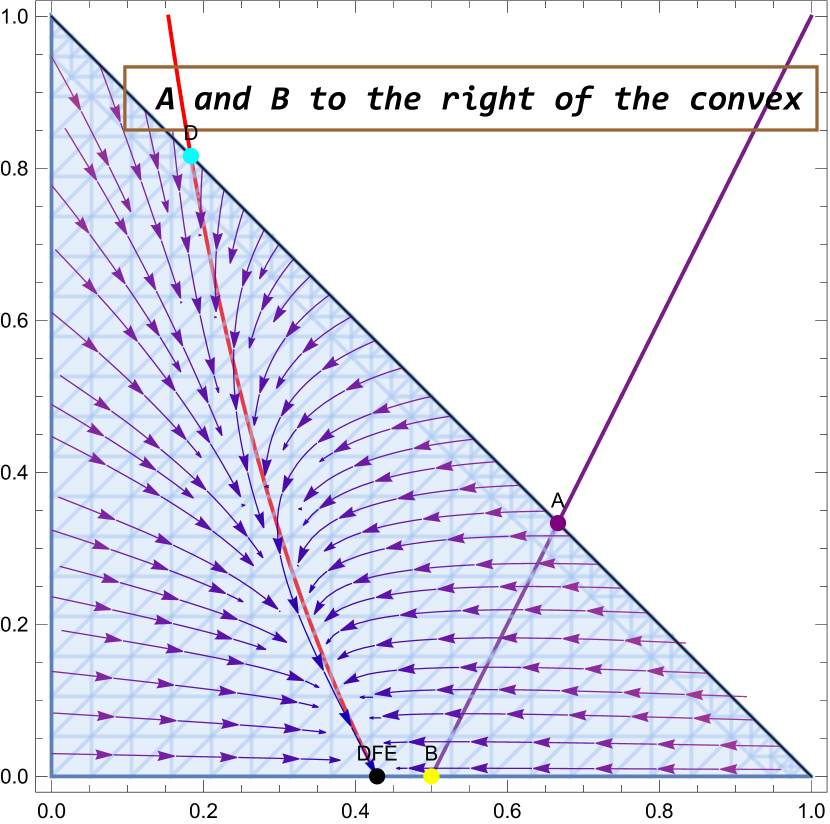
(a) ${\mathcal{R}}_{0}=0.952381<1,\beta=4,\beta_{r}=2,\Lambda+\gamma+\nu_{i}=1+1+1=3,\beta_{r}^{(+)}=1.625,\gamma_{r}=1/2,\gamma_{s}=2,\beta_{r}<\Lambda+\nu_{i}+\gamma<\beta,\nu_{i}<\beta,\beta_{r}>\beta_{r}^{(+)},\;\text{and}\;\gamma_{s}>\gamma_{s}^{*}\Leftrightarrow s_{B}>s_{dfe}$.

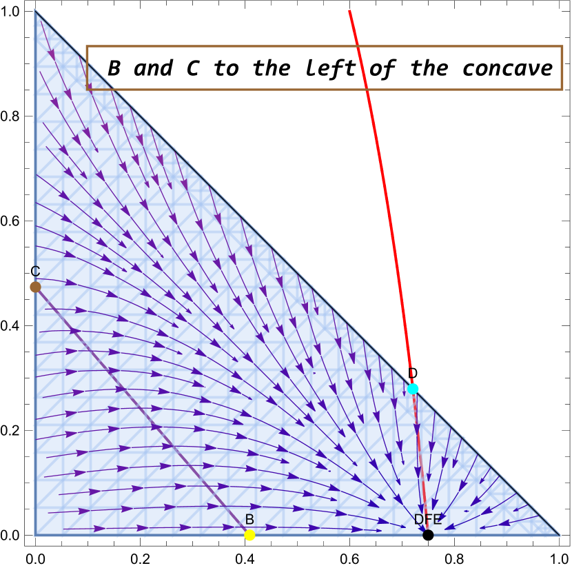
(b) $\beta=0.03,\beta_{r}=0.25,\Lambda+\gamma+\nu_{i}=0.03+0.07+0.06=0.16,\beta_{r}^{(+)}=0.0219597,\gamma_{r}=0.03,\gamma_{s}=0,02,\beta<\nu_{i}<\Lambda+\nu_{i}+\gamma<\beta_{r},\beta_{r}>\beta_{r}^{(+)},\;\text{and}\;\gamma_{s}<\gamma_{s}^{*}\Leftrightarrow s_{B}<s_{dfe}$.

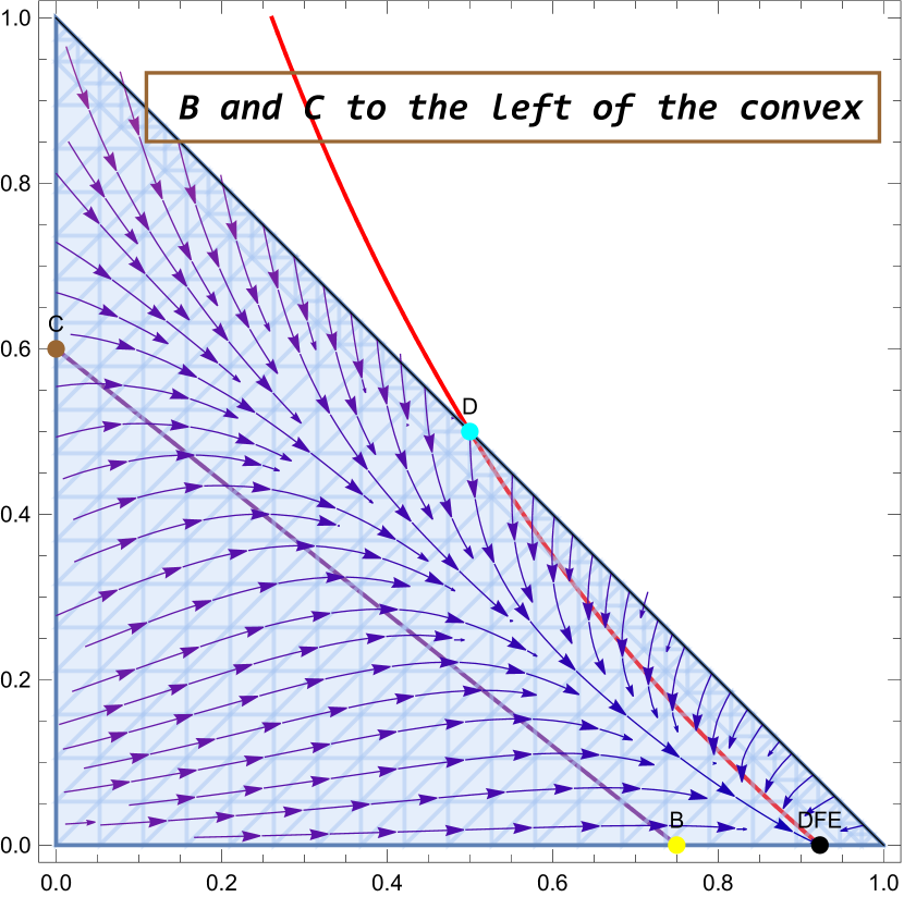
(c) $\beta=0.1,\beta_{r}=0.3,\Lambda+\gamma+\nu_{i}=0.03+0.07+0.05=0.15,\beta_{r}^{(+)}=0.729883,\gamma_{r}=0.03,\gamma_{s}=0,02,\nu_{i}<\beta<\Lambda+\nu_{i}+\gamma\leq\beta_{r},\beta_{r}<\beta_{r}^{(+)},\;\text{and}\;\gamma_{s}<\gamma_{s}^{*}\Leftrightarrow s_{B}<s_{dfe}$.

(d) $\beta=0.2,\beta_{r}=0.4,\Lambda+\gamma+\nu_{i}=0.01+0.07+0.15=0.23,\beta_{r}^{(+)}=0.327443,\gamma_{r}=10^{-4},\gamma_{s}=0,002,\nu_{i}<\beta<\Lambda+\gamma+\nu_{i}<\beta_{r},\beta_{r}\geq\beta_{r}^{(+)},\;\text{and}\;s_{B}<s_{dfe}$.

(e) $\Lambda+\gamma+\nu_{i}=1+2.1+0.1=3.2>\beta_{r}=3.1>\beta=3,\gamma_{r}=0.1,\gamma_{s}=0.3,\beta<\beta_{r}<\Lambda+\gamma+\nu_{i},\;\text{and}\;\beta>\nu_{i}$.

(f) $\Lambda+\gamma+\nu_{i}=1+1+2.5=4.5>\beta=0.5>\beta_{r}=0.25,\gamma_{r}=1,\gamma_{s}=1,\beta_{r}<\beta<\Lambda+\gamma+\nu_{i},\;\text{and}\;\beta<\nu_{i}$.

Figure 6: Stream plots of $(\;\mathsf{s},\;\mathsf{i})$ when $\gamma_{s}>0$, in six cases when ${\mathcal{R}}_{0}<1$. The DFE is the only stable sink in the boundary of the domain, with the exception of case (d), when EE1=($0.313823,0.428942$) is a second sink, and EE2=($0.799177,0.0406582$) is a saddle point.

In practical situations, certain parameter relations, for instance $\beta_{r}>\beta,\nu_{r}>\nu_{i},$ might seem “unreasonable from a medical point of view”. In what follows, we choose not to assume any relationship among the parameters in (1) in order to highlight the fact surprising mathematical behaviors like bistability– see Figure 6(d) – may arise when “things go wrong”.

We make now several remarks, which serve as an appetizer for the rest of the paper.

Remark 3.

The critical value $\beta=\beta_{r}$ defines a model where both the sickness and the vaccination do not affect the infectivity (neither confers any immunity). The recovered class might be better viewed then as a susceptible class $S_{o}$ of older individuals, with extra mortality rate $\nu_{r}>0$ and no births:

$$S^{\prime}(t) =\Lambda N(t)-\frac{\beta}{N(t)}S(t)I(t)-(\gamma_{s}+\mu)S(t)+\gamma_{r}S_{o}(t),$$

$$S_{o}^{\prime}(t) =-\frac{\beta}{N(t)}S_{o}(t)I(t)-(\gamma_{r}+\mu+\nu_{r})S_{o}(t)+\gamma_{s}S(t)+\gamma I(t),$$

$$I^{\prime}(t) =I(t)\left(\frac{\beta}{N(t)}\left(S(t)+S_{o}(t)\right)-\gamma-\mu-\nu_{i}\right).$$

A moment of reflection reveals that this particular case has two surprising features: a) after the infection is over, transfers only occur towards the old class $S_{o}$, and b) transfers between the two age groups occur; it is hard to make sense of this, without further imposing $\gamma_{s}=\gamma_{r}=0$.

Remark 4.

When $\beta_{r}=0$, our model is an example of matrix-SIR Arino model with linear birth rate, a class of models for which only few general results are available AAB⁺ (21).

In what follows, we will investigate the stability properties of an equivalent system to (1) obtained by investigating the normalized quantities $\;\mathsf{s}=\frac{S}{N},\;\mathsf{i}=\frac{I}{N},\;\mathsf{r}=\frac{R}{N}$ and given by (see Proposition 1, Section 2 for a detailed derivation).

$$\begin{cases}&\;\mathsf{s}^{\prime}(t)=\Lambda+\gamma_{r}\;\mathsf{r}(t)-\left(\beta\;\mathsf{i}(t)+\gamma_{s}\right)\;\mathsf{s}(t)+\;\mathsf{s}(t)(-\Lambda+\nu_{i}\;\mathsf{i}(t)+\nu_{r}\;\mathsf{r}(t)),\\ &\;\mathsf{i}^{\prime}(t)=\;\mathsf{i}(t)\left[\beta\;\mathsf{s}(t)+\nu_{i}\;\mathsf{i}(t)+(\nu_{r}+\beta_{r})\;\mathsf{r}(t)-\left(\gamma+{\nu_{i}+\Lambda}\right)\right],\\ &\;\mathsf{r}^{\prime}(t)=\gamma\;\mathsf{i}(t)+\gamma_{s}\;\mathsf{s}(t)-{(\gamma_{r}+\Lambda+\nu_{r})}\;\mathsf{r}(t)+\;\mathsf{r}(t)(-\beta_{r}\;\mathsf{i}(t)+\nu_{i}\;\mathsf{i}(t)+\nu_{r}\;\mathsf{r}(t)),\\ &\;\mathsf{s}(t)+\;\mathsf{i}(t)+\;\mathsf{r}(t)=1.\end{cases}$$

Remark 5.

Note this reduces to the classic SIR model KM (27) when $\Lambda=\nu_{i}=\nu_{r}=\gamma_{r}=\gamma_{s}=\beta_{r}=0$.

Remark 6.

Factoring the second equation reveals the threshold after which the infection starts decreasing

$$\beta\;\mathsf{s}(t)+\nu_{i}\;\mathsf{i}(t)+(\nu_{r}+\beta_{r})\;\mathsf{r}(t)<\Lambda+\gamma+\nu_{i}$$ (1.2)

herd immunity $(\;\mathsf{s},\;\mathsf{i})$ line, or max-line (line since $\;\mathsf{r}=1-\;\mathsf{s}-\;\mathsf{i}$). Notice that, in contrast with the case of models with constant population size and no loss of immunity where the herd immunity condition depends only on the susceptible state, the above condition depends on three states $(\;\mathsf{s},\;\mathsf{i},\;\mathsf{r})$. Also, when $\nu_{i}=\nu_{r}=\beta_{r}=0$, this reduces to the well-studied herd immunity threshold.

1) The inequality obtained at the DFE, when $\;\mathsf{i}=0$,

$$\beta s_{dfe}+(\nu_{r}+\beta_{r})r_{dfe}\leq\Lambda+\gamma+\nu_{i}\Leftrightarrow\frac{\beta s_{dfe}+(\nu_{r}+\beta_{r})r_{dfe}}{\Lambda+\gamma+\nu_{i}}:={\mathcal{R}}_{0}<1$$ (1.3)

turns out to ensure the local stability of the disease free equilibrium (disease free equilibrium)  – see section 3.

2) ${\mathcal{R}}_{0}$ introduced above coincides with the famous basic reproduction number defined via the next generation matrix approach.

3) The disease free equilibrium (obtained by plugging $\;\mathsf{i}=0,\;\mathsf{r}=1-\;\mathsf{s}$ in the fixed point equation) is such that

$$s_{dfe}:=\frac{\Lambda+\gamma_{r}}{\Lambda+\gamma_{r}+\gamma_{s}}\in[0,1],\quad s_{dfe}=1\Leftrightarrow\gamma_{s}=0$$ (1.4)

Remark 7.

A) The equality ${\mathcal{R}}_{0}=1$ is linear in $\gamma_{s}$ and yields the so called “critical vaccination”

$${\gamma_{s}^{*}}=\left(\Lambda+\gamma_{r}\right)\frac{\beta-\left(\Lambda+\gamma+\nu_{i}\right)}{\Lambda+\gamma+\nu_{i}-\beta_{r}},$$ (1.5)

provided that the denominator doesn’t blow-up.

This formula is positive if either $\beta_{r}\leq\Lambda+\gamma+\nu_{i}\leq\beta$, or $\beta\leq\Lambda+\gamma+\nu_{i}\leq\beta_{r}$. When $\beta_{r}=0$, we recover a classical critical vaccination formula

$${\gamma_{s}^{*}}=\left(\Lambda+\gamma_{r}\right)\left(\mathcal{R}-1\right),\mathcal{R}=\frac{\beta}{\Lambda+\gamma+\nu_{i}}.$$ (1.6)

B) The equality ${\mathcal{R}}_{0}=1$ is also linear in $\beta$ and yields a “critical contact rate ”

$$\beta^{*}=\frac{\left(\gamma+\nu_{i}+\Lambda\right)\left(\Lambda+\gamma_{r}+\gamma_{s}\right)-\beta_{r}\gamma_{s}}{\Lambda+\gamma_{r}}.$$ (1.7)

It may be checked that at this critical value the value $i_{ee}$ of the infectious at the lower endemic point crosses the $i=0$ axis, and may reduce the number of endemic points from 3 to 2 – see Figure 7 for details.

Contents. Section 2 reviews the dimension reduction available for the proportions of models with linear birth rate, and emphasizes the fact that the well studied deterministic model is an approximation of the model with linear birth rate studied here. A second, finer “intermediate approximation” is introduced as well.

Section 3 computes ${\mathcal{R}}_{0}$ via the next generation matrix approach (NGM), establishing thereby the well-known weak ${\mathcal{R}}_{0}$ alternative VdDW (08); it also introduces the concept of “strong global stability” of the DFE in Proposition 4, which may be useful for more advanced models.

The endemic equilibria are discussed in Section 4.

Section 5 identifies more precisely, in the particular case $\nu_{r}=0$, the case when global stability does not hold. The results involve heavily the vaccination parameter $\gamma_{s}$ and its critical value. The increased complexity of the model forces a geometric approach, already hinted at in (DvdD, 93, Sec. 4). This ends up in the consideration of 10 cases, one of which, Theorem 52.(c), remains only partly resolved.

Section 6 discusses the particular case $\gamma_{s}=0$, generalizing and providing missing details of the results in (DvdD, 93, Sec. 4).

Section 7 gives the simpler results for the first approximation FA (actually for a slightly more general “classic/pedagogical model”).

Finally, Section 8 provides the proof of a technical result, and Section 9 reviews the pillar of deterministic epidemic models: the definition of the basic reproduction number via the next generation matrix method.

2 Dimension reduction for the SIR/V+S model with linear birth rate

It is convenient to reformulate (1) in terms of the normalized fractions

$$\;\mathsf{s} =\frac{S}{N}, \;\mathsf{i} =\frac{I}{N}, \;\mathsf{r} =\frac{R}{N}.$$ (2.1)

This process, sometimes called “non-dimensionalizing” (see for example  Ras (21)), allows us to provide the following equivalent representation of (1).

Proposition 1.

Let $\;\mathsf{s},\;\mathsf{i},\;\mathsf{r}$ be as defined in (2.1). Then, the dynamics (1) can be equivalently rewritten as:

$$\;\mathsf{s}^{\prime}(t) =\Lambda+\gamma_{r}\;\mathsf{r}(t)-\left(\beta\;\mathsf{i}(t)+\gamma_{s}\right)\;\mathsf{s}(t)+\;\mathsf{s}(t)(-\Lambda+\nu_{i}\;\mathsf{i}(t)+\nu_{r}\;\mathsf{r}(t)),$$

$$\;\mathsf{i}^{\prime}(t) =\;\mathsf{i}(t)\left[\beta\;\mathsf{s}(t)+\nu_{i}\;\mathsf{i}(t)+(\nu_{r}+\beta_{r})\;\mathsf{r}(t)-\left(\gamma+{\nu_{i}+\Lambda}\right)\right],$$

$$\;\mathsf{r}^{\prime}(t) =\gamma\;\mathsf{i}(t)+\gamma_{s}\;\mathsf{s}(t)-{(\gamma_{r}+\Lambda+\nu_{r})}\;\mathsf{r}(t)+\;\mathsf{r}(t)(-\beta_{r}\;\mathsf{i}(t)+\nu_{i}\;\mathsf{i}(t)+\nu_{r}\;\mathsf{r}(t)),$$

$$\;\mathsf{s}(t) +\;\mathsf{i}(t)+\;\mathsf{r}(t)=1.$$ (2.2)

Proof. By using

$$N^{\prime}(t)/N(t)=(\Lambda-\mu)-\nu_{i}\;\mathsf{i}(t)-\nu_{r}\;\mathsf{r}(t),$$ (2.3)

we obtain for the susceptibles:

$$\;\mathsf{s}^{\prime}(t) =\frac{S^{\prime}}{N}-\frac{N^{\prime}}{N^{2}}S$$

$$=\frac{\Lambda(N)}{N}-\frac{\beta S(t)I(t)}{N^{2}}+\frac{\gamma_{r}R(t)-(\mu+\gamma_{s})S(t)}{N}-S(t)\frac{(\Lambda-\mu)-\nu_{i}\;\mathsf{i}(t)-\nu_{r}\;\mathsf{r}(t)}{N}$$

$$=\Lambda(1-\;\mathsf{s}(t))-\beta\;\mathsf{s}(t)\;\mathsf{i}(t)+\gamma_{r}\;\mathsf{r}(t)+\;\mathsf{s}(t)\left(\mu+\nu_{i}\;\mathsf{i}(t)+\nu_{r}\;\mathsf{r}(t)-\mu-\gamma_{s}\right)$$

$$=\Lambda-\beta\;\mathsf{s}(t)\;\mathsf{i}(t)+\gamma_{r}\;\mathsf{r}(t)-{(\gamma_{s}+\Lambda)}\;\mathsf{s}(t)+\;\mathsf{s}(t)(\nu_{i}\;\mathsf{i}(t)+\nu_{r}\;\mathsf{r}(t)).$$

Similarly,

$$\;\mathsf{i}^{\prime}(t) =\frac{I^{\prime}}{N}-\frac{N^{\prime}}{N^{2}}I=\beta\;\mathsf{s}(t)\;\mathsf{i}(t)-(\gamma+\mu+\nu_{i})\;\mathsf{i}(t)-I(t)\frac{(\Lambda-\mu)-\nu_{i}\;\mathsf{i}(t)-\nu_{r}\;\mathsf{r}(t)}{N}$$

$$=-\;\mathsf{i}(t)\Lambda+\;\mathsf{i}(t)(\beta\;\mathsf{s}(t)+\beta_{r}\;\mathsf{r}(t))-(\gamma+\mu+\nu_{i})\;\mathsf{i}(t)+\;\mathsf{i}(t)\left(\mu+\nu_{i}\;\mathsf{i}(t)+\nu_{r}\;\mathsf{r}(t)\right)$$

$$=\;\mathsf{i}(t)\left[\beta\;\mathsf{s}(t)+\nu_{i}\;\mathsf{i}(t)+(\beta_{r}+\nu_{r})\;\mathsf{r}(t)-\left(\Lambda+\gamma+\nu_{i}\right)\right],$$

and

$$\;\mathsf{r}^{\prime}(t) =\frac{R^{\prime}}{N}-\frac{N^{\prime}}{N^{2}}R$$

$$=\gamma\;\mathsf{i}(t)+\gamma_{s}\;\mathsf{s}(t)-(\gamma_{r}+\mu+\nu_{r})\;\mathsf{r}(t)-R(t)\frac{(\Lambda-\mu)-\nu_{i}\;\mathsf{i}(t)-\nu_{r}\;\mathsf{r}(t)}{N}$$

$$=\gamma\;\mathsf{i}(t)+\gamma_{s}\;\mathsf{s}(t)-{(\gamma_{r}+\Lambda+\nu_{r})}\;\mathsf{r}(t)+\;\mathsf{r}(t)(-\beta_{r}\;\mathsf{i}(t)+\nu_{i}\;\mathsf{i}(t)+\nu_{r}\;\mathsf{r}(t)).$$

Finally, $\;\mathsf{s}(t)+\;\mathsf{i}(t)+\;\mathsf{r}(t)=1$ follows from $N^{\prime}(t)=(S(t)+I(t)+R(t))^{\prime}$ by substituting (2.1), which proves the equivalence between (1) and (1). $\blacksquare$

Remark 8.

Note that the natural death rate $\mu$ does not intervene in (1), which is to be expected. Indeed, since this rate is the same for all the compartments, it has no effect on the fractions.

Remark 9.

1. Note that the conservation equation

   $$\mathsf{n}:=\;\mathsf{s}+\;\mathsf{i}+\;\mathsf{r}=1,$$

   in general, does not follow from the first three equations in (1). Indeed, by summing the right hand-sides we have:

   $$\mathsf{n}^{\prime}(t)=\left[1-\;\mathsf{s}(t)-\;\mathsf{r}(t)-\;\mathsf{i}(t)\right](\Lambda-\nu_{i}\;\mathsf{i}(t)-\nu_{r}\;\mathsf{r}(t)),$$

   which shows that $\mathsf{n}^{\prime}(t)\neq 0$ in general cases. However, the above differential equation guarantees that if $\;\mathsf{s}(t_{0})+\;\mathsf{i}(t_{0})+\;\mathsf{r}(t_{0})=1$ for some $t_{0}\in\mathbb{R}_{\geq 0}$, then $\;\mathsf{s}(t)+\;\mathsf{i}(t)+\;\mathsf{r}(t)=1$ for all $t\geq t_{0}$. Accordingly, the manifold

   $$\mathcal{D}:=\{\;\mathsf{s}+\;\mathsf{i}+\;\mathsf{r}=1,\;\mathsf{s}\geq 0,\;\mathsf{i}\geq 0,\;\mathsf{r}\geq 0\}$$

   is forward-invariant, since the flow along its boundaries is directed towards the interior – see Raz (01) . Note that the conservation equation may replace either the last or the first equation in the dynamics, and allows reducing the computation of fixed points to dimension $2$.

2. The Jacobian matrix of (1) is given by

   $$J(s,i)=\left(\begin{array}[]{cc}i\left(\nu_{i}-\beta\right)-\Lambda-\gamma_{r}-\gamma_{s}&s\left(\nu_{i}-\beta\right)-\gamma_{r}\\ i\left(\beta-\beta_{r}\right)&-\gamma+2i\nu_{i}-\nu_{i}-2i\beta_{r}-\Lambda+\beta_{r}+s\left(\beta-\beta_{r}\right)\\ \end{array}\right).$$ (2.4)

   Following LGWK (99), let us investigate when this system is order preserving in the interior of the convex feasible region $\mathcal{D}$. The Jacobian (2.4) is a Metzler matrix $\forall(s,i)\in\mathcal{D}$ iff $\nu_{i}-\beta-\gamma_{r}>0,\gamma_{r}\leq 0,\beta>\beta_{r}\Leftrightarrow\nu_{i}>\beta+\gamma_{r},\gamma_{r}\leq 0,\beta>\beta_{r}$. Thus, if $\begin{cases}\nu_{i}>\beta+\gamma_{r}\\ \gamma_{r}\leq 0\\ \beta>\beta_{r}\end{cases},$ the system (1) is order preserving with respect to  the partial ordering defined by the orthant $\left\{(s,i)\in\mathbb{R}^{2},\;s\geq 0,\;i\geq 0\right\}$.

   

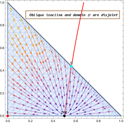
   Figure 1: Stream Plot of $(\;\mathsf{s},\;\mathsf{i})$ when $\nu_{i}>\beta+\gamma_{r},\gamma_{r}=0,\beta>\beta_{r}$, with $\beta=\frac{1}{2},\beta_{r}=\frac{1}{4},\Lambda=1,\nu_{i}=1.01,\gamma=1,\gamma_{r}=0,\gamma_{s}=1$. The DFE is a stable sink.

   Analogously, if $\begin{cases}\nu_{i}<\beta+\gamma_{r}\\ \gamma_{r}>0\\ \beta<\beta_{r}\end{cases},$ the system (1) is order preserving with respect to  the partial ordering defined by the orthant $\left\{(s,i)\in\mathbb{R}^{2},\;s\leq 0,\;i\geq 0\right\}$.

   

   (a) ${\mathcal{R}}_{0}<1$, with $\beta=1.01,\beta_{r}=2,\Lambda=1,\nu_{i}=1,\gamma=1,\gamma_{r}=1,\gamma_{s}=1$, the DFE is a stable sink.

   

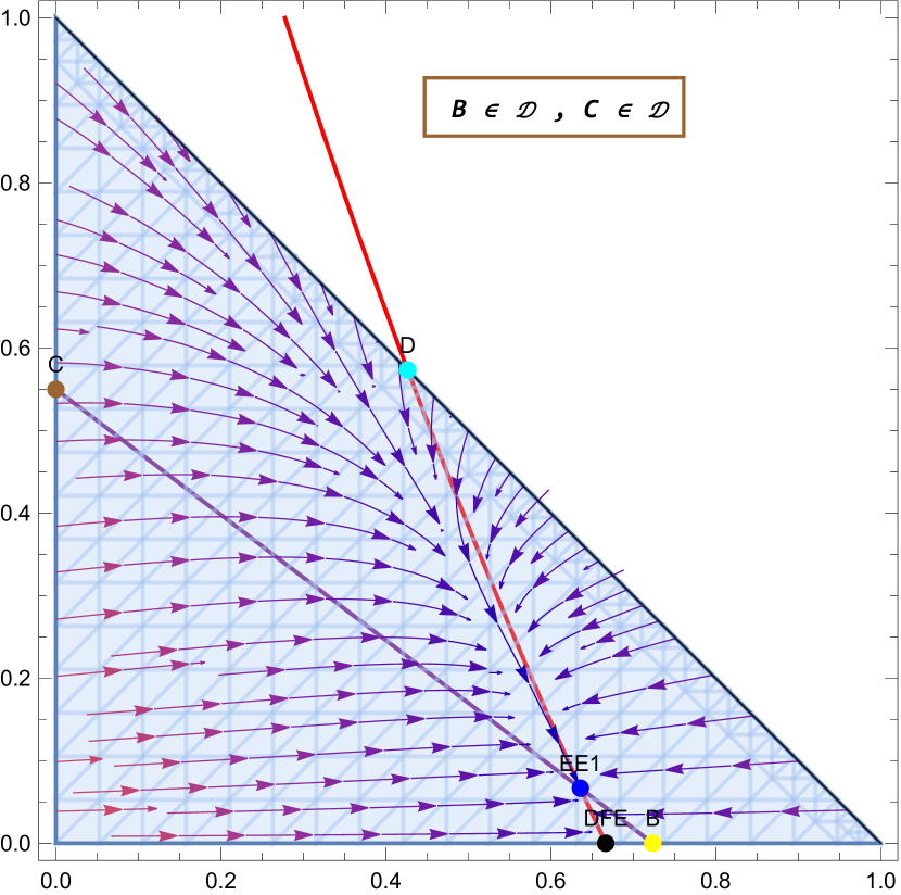
   (b) $B,C\in\mathcal{D},{\mathcal{R}}_{0}>1$, with $\beta=1.1,\beta_{r}=3,\Lambda=1,\nu_{i}=\frac{1}{2},\gamma=\frac{1}{8},\gamma_{r}=1,\gamma_{s}=1$, The DFE is a saddle point and EE is a stable sink.

   Figure 2: Stream Plot of $(\;\mathsf{s},\;\mathsf{i})$ when $\nu_{i}<\beta+\gamma_{r},\gamma_{r}>0,\beta<\beta_{r}$.

The study of the dynamics in Proposition 1 is quite challenging, and it may be useful sometimes to consider also the two approximations introduced in the following definition.

Definition 1.

Let $\Phi_{s},\Phi_{i},\Phi_{r}\in\{0,1\}$ and let

$$\;\mathsf{s}^{\prime}(t) =\Lambda-\beta\;\mathsf{s}(t)\;\mathsf{i}(t)+\gamma_{r}\;\mathsf{r}(t)-{(\gamma_{s}+\Lambda)}\;\mathsf{s}(t)+\Phi_{s}\;\mathsf{s}(t)(\nu_{i}\;\mathsf{i}(t)+\nu_{r}\;\mathsf{r}(t)),$$

$$\;\mathsf{i}^{\prime}(t) =\;\mathsf{i}(t)\left[\beta\;\mathsf{s}(t)+\beta_{r}\;\mathsf{r}(t)-\left(\gamma+{\nu_{i}+\Lambda}\right)\right]+\Phi_{i}\;\mathsf{i}(t)(\nu_{i}\;\mathsf{i}(t)+\nu_{r}\;\mathsf{r}(t)),$$

$$\;\mathsf{r}^{\prime}(t) =\gamma\;\mathsf{i}(t)+\gamma_{s}\;\mathsf{s}(t)-{(\gamma_{r}+\Lambda+\nu_{r})}\;\mathsf{r}(t)-\beta_{r}\;\mathsf{r}(t)\;\mathsf{i}(t)+\Phi_{r}\;\mathsf{r}(t)(\nu_{i}\;\mathsf{i}(t)+\nu_{r}\;\mathsf{r}(t)),$$

$$\;\mathsf{s}(t) +\;\mathsf{i}(t)+\;\mathsf{r}(t)=1.$$ (2.5)

1. The model (1) with $\Phi_{s}=\Phi_{i}=\Phi_{r}=1$ will be called scaled model (SM).

2. The model (1) with $\Phi_{s}=\Phi_{i}=\Phi_{r}=0$ will be called first approximation (FA) in the specific case $\Lambda=\mu$. The FA is thus:

   $$\;\mathsf{s}^{\prime}(t) =\Lambda-\beta\;\mathsf{s}(t)\;\mathsf{i}(t)+\gamma_{r}\;\mathsf{r}(t)-{(\gamma_{s}+\Lambda)}\;\mathsf{s}(t),$$

   $$\;\mathsf{i}^{\prime}(t) =\;\mathsf{i}(t)\left[\beta\;\mathsf{s}(t)+\beta_{r}\;\mathsf{r}(t)-\left(\gamma+{\nu_{i}+\Lambda}\right)\right],$$

   $$\;\mathsf{r}^{\prime}(t) =\gamma\;\mathsf{i}(t)+\gamma_{s}\;\mathsf{s}(t)-{(\gamma_{r}+\Lambda+\nu_{r})}\;\mathsf{r}(t)-\beta_{r}\;\mathsf{r}(t)\;\mathsf{i}(t),$$

   $$\;\mathsf{s}(t) +\;\mathsf{i}(t)+\;\mathsf{r}(t)=1.$$ (2.6)

3. The model (1) with $\Phi_{s}=\Phi_{r}=1$ and $\Phi_{i}=0$ will be called intermediate approximation (IA).

Remark 10.

Each model, in particular SIR/V+S, has a SM, FA and IA version, which will be denoted by SIR/V+S-SM, SIR/V+S-FA, SIR/V+S-IA.

Remark 11.

The FA is not a constant population model when $\nu_{c}>0$, for some compartment $c$.

Remark 12.

It follows from $N^{\prime}(t)/N(t)=(\Lambda-\mu)-\nu_{i}\;\mathsf{i}(t)-\nu_{r}\;\mathsf{r}(t)$ that $N^{\prime}(t)=0$ for all $t\in\mathbb{R}_{\geq 0}$ if and only if $\mu=\Lambda$ and $\nu_{i}=\nu_{r}=0$. Thus, the popular assumption of constant population size Het (76) applies only to epidemics without extra-deaths, which contradicts the essence of most epidemics (BCCF, 19, Ch. 10.2). Clearly, constant population papers have in mind some large $N$ or short term approximation, but this is rather vague. On the other hand, the FA approximation (2) with $\mu=\Lambda$, as well as IA, may be heuristically justified as approximations obtained by ignoring certain quadratic terms in (1). This justifies studying FA without restrictive assumptions like $\nu_{i}=0$.

Remark 13.

A considerable part of the epidemics literature studies (1) with $N(t)=1$ (this produces an analog of (2) with $\mu\neq\Lambda$). The justification for studying this model is of course an assumption that $N$ is “approximately constant”. The purpose of our paper is not to assume that; however, we chose to include results about them, under the name “classic/pedagogic models” (PM), to be in line with this part of the literature. As explained, we need here only results on the FA model (which approximate the object of interest to us (1)), and these may be easily recovered by replacing $\mu$ with $\Lambda$.

We conclude this section by illustrating in Figure 3 a comparison between the trajectories of the first approximation, of the intermediate approximation, and of the scaled model. Note that the approximate dynamics are an accurate approximation of the SM at the beginning of the epidemic (i.e., when $\;\mathsf{i}(t)\approx 0$). This period starts with the lower part in Figure 3, and continues until the processes start turning towards their distinct endemic points – see JKKPS (21) for a rigorous slow-fast analysis of similar models.

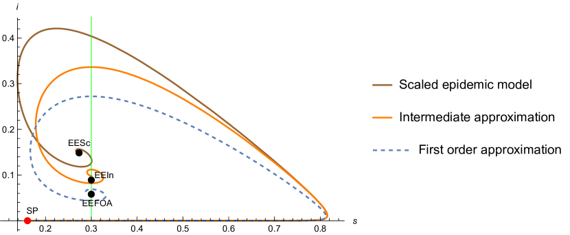
Figure 3: Parametric $(\;\mathsf{s},\;\mathsf{i})$ plots of the scaled epidemic (1) and its FA (2) and intermediate approximations for a SIR-type model with one infectious class, starting from a starting point SP with $i_{0}=10^{-6},\mathcal{R}_{0}=3.21,$ critical vaccination $0.622222$, and $\gamma_{s}=.01$. The other parameters are $\beta=5,\;\gamma=1/2,\;\Lambda=\mu=1/10,\;\gamma_{r}=1/6,\;\nu_{i}=.9,\;\nu_{r}=0$. $EESc,EEIn,EEF0A$ are the stable endemic points of the scaled model, intermediate model, and the FA model, respectively. The green vertical line denotes the immunity threshold $1/\mathcal{R}=s_{EEF0A}=s_{EEIn}.$ Note that the epidemic will spend at first a long time (since births and deaths have slow rates as compared to the disease) in the vicinity of the manifold $\vec{\;}\mathsf{i}(t)=0$, where the three processes are indistinguishable, before turning towards the endemic equilibrium point(s).

2.1 The disease free system and its equilibria

It is convenient to eliminate $\;\mathsf{r}$ from $\;\mathsf{s}+\;\mathsf{i}+\;\mathsf{r}=1$, and work with the following two-dimensional scaled dynamic

$$\begin{cases}\;\mathsf{s}^{\prime}(t)=\Lambda-\;\mathsf{s}(t)\;\mathsf{i}(t)(\beta-\nu_{i})-(\gamma_{s}+\Lambda)\;\mathsf{s}(t)+(\gamma_{r}+\nu_{r}\;\mathsf{s}(t))(1-\;\mathsf{s}(t)-\;\mathsf{i}(t))\\ \;\mathsf{i}^{\prime}(t)=\;\mathsf{i}(t)\left[\;\mathsf{s}(t)\beta+\nu_{i}\;\mathsf{i}(t)+(\nu_{r}+\beta_{r})(1-\;\mathsf{s}(t)-\;\mathsf{i}(t))\right]-\;\mathsf{i}(t)\left(\Lambda+\gamma+\nu_{i}\right)\end{cases},$$ (2.7)

defined on the positively invariant region Raz (01)

$$\mathcal{D}=\left\{(s,i),\;s\geq 0,\;i\geq 0,\;s+i\leq 1\right\}.$$

The fixed points are the solutions of

$$\begin{cases}\;\mathsf{s}\left[\nu_{r}\;\mathsf{s}+\;\mathsf{i}(\beta-\nu_{i}+\nu_{r})+\Lambda+\gamma_{s}+\gamma_{r}-\nu_{r}\right]+\;\mathsf{i}\gamma_{r}-(\Lambda+\gamma_{r})=0\\ \;\mathsf{i}\left[\;\mathsf{s}(\beta-\nu_{r}-\beta_{r})+(\nu_{i}-\nu_{r}-\beta_{r})\;\mathsf{i}+\nu_{r}+\beta_{r}-(\Lambda+\gamma+\nu_{i})\right]=0\end{cases}.$$ (2.8)

The disease free system ( with $\;\mathsf{i}=0,\;\mathsf{r}=1-\;\mathsf{s}$) reduces to

$$\begin{split}\;\mathsf{s}^{\prime}(t)=\Lambda-(\gamma_{s}+\Lambda)\;\mathsf{s}(t)+(\gamma_{r}+\nu_{r}\;\mathsf{s}(t))(1-\;\mathsf{s}(t))\\ =\Lambda+\gamma_{r}-(\gamma_{s}+\gamma_{r}+\Lambda-\nu_{r})\;\mathsf{s}(t)-\nu_{r}\;\mathsf{s}(t)^{2},\end{split}$$ (2.9)

and its fixed points are such that $\;\mathsf{s}$ satisfies  the equation

$$\begin{cases}\Lambda+\gamma_{r}-\;\mathsf{s}\left[\nu_{r}\;\mathsf{s}+\Lambda+\gamma_{r}+\gamma_{s}-\nu_{r}\right]=0&\nu_{r}>0\\ \;\mathsf{s}\left[\Lambda+\gamma_{r}+\gamma_{s}\right]-(\Lambda+\gamma_{r})=0&\nu_{r}=0\end{cases}.$$

One root

$$s_{dfe}=\begin{cases}\frac{\Lambda+\gamma_{r}}{\Lambda+\gamma_{r}+\gamma_{s}}&\nu_{r}=0\\ \frac{\sqrt{\Delta_{dfe}}-\left(\Lambda+\gamma_{r}+\gamma_{s}-\nu_{r}\right)}{2\nu_{r}},\quad\Delta_{dfe}=4\nu_{r}\left(\Lambda+\gamma_{r}\right)+\left(\Lambda+\gamma_{r}+\gamma_{s}-\nu_{r}\right)^{2}&\nu_{r}>0\end{cases}$$ (2.10)

is always in $[0,1]$ and will be denoted by $s_{dfe}$.

Remark 14.

$s_{dfe}$ is continuous in $\nu_{r}$, since for $\nu_{r}$ small,

$$s_{dfe}\approx\frac{\Lambda+\gamma_{r}+\gamma_{s}-\nu_{r}+\frac{2\nu_{r}\left(\Lambda+\gamma_{r}\right)}{\Lambda+\gamma_{r}+\gamma_{s}-\nu_{r}}-\left(\Lambda+\gamma_{r}+\gamma_{s}-\nu_{r}\right)}{2\nu_{r}}\to\frac{\Lambda+\gamma_{r}}{\Lambda+\gamma_{r}+\gamma_{s}}$$

Remark 15.

The other root in the quadratic case $\nu_{r}>0$

$$\frac{\nu_{r}-\left(\Lambda+\gamma_{r}+\gamma_{s}\right)-\sqrt{4\nu_{r}\left(\Lambda+\gamma_{r}\right)+\left(\Lambda+\gamma_{r}+\gamma_{s}-\nu_{r}\right)^{2}}}{2\nu_{r}}$$ (2.11)

is strictly negative, unless

$$\begin{cases}\Lambda+\gamma_{r}=0\\ \nu_{r}\geq\gamma_{s}+\Lambda+\gamma_{r}\end{cases}\Leftrightarrow\begin{cases}\Lambda=\gamma_{r}=0\\ \nu_{r}\geq\gamma_{s}\end{cases},$$ (2.12)

in which case it yields a second DFE point with $\;\mathsf{s}=0=\;\mathsf{i}$.

Assumption 1.

We will exclude from now on the particular boundary case (2.12), which may be resolved by elementary explicit eigenvalues computations – see Raz (01) .

Once this case is removed, the DFE is unique, and we may apply the next generation matrix method, the first step of which consists in checking the local asymptotic stability of $s_{dfe}$ for the disease-free equation (2.9).

In our case, this amounts to proving that

$$\lambda_{-}:=\nu_{r}-(\Lambda+\gamma_{r}+\gamma_{s})-2\nu_{r}s_{dfe}<0.$$ (2.13)

This is automatic both when $\nu_{r}=0$, and when $\nu_{r}>0,$ since by (2.10) $\lambda_{-}=-\sqrt{\Delta_{dfe}}<0$.

3 Local DFE stability via the next generation matrix approach vdDW (02)

Recall (cf. Assumption 1) that we exclude the case $\Lambda=\gamma_{r}=0,\nu_{r}\geq\gamma_{s}$ (2.12), so that the DFE defined in (2.10) is unique and locally stable in the disease free space (2.13), so that the next generation matrix approach may be attempted.

This proceeds in the following steps:

1. Separate the “infected equation” for $\;\mathsf{i}$ (1) as a difference of two terms, $\mathcal{F},\mathcal{V}$, as follows

   $$\;\mathsf{i}^{\prime}(t) =\;\mathsf{i}(t)\left[\;\mathsf{s}(t)\beta+(\nu_{r}+\beta_{r})(1-\;\mathsf{s}(t)-\;\mathsf{i}(t))\right]-\;\mathsf{i}(t)\left[\Lambda+\gamma+\nu_{i}-\nu_{i}\;\mathsf{i}(t)\right]$$

   $$=\mathcal{F}(s,i)-\mathcal{V}(i)$$

   where $\begin{cases}\mathcal{F}(s,i):=\;\mathsf{i}(t)\left[\;\mathsf{s}(t)\beta+(\nu_{r}+\beta_{r})(1-\;\mathsf{s}(t)-\;\mathsf{i}(t))\right]\\ \mathcal{V}(i):=\;\mathsf{i}(t)\left[\Lambda+\gamma+\nu_{i}+\nu_{i}\;\mathsf{i}(t)\right]\end{cases}.$ The necessary decomposition conditions on $\mathcal{F},\mathcal{V}$ (9.2) are immediate, and the gradients

   $$F=\left[\frac{\partial\mathcal{F}}{\partial\;\mathsf{i}}\right]_{i=0,s=s_{dfe}}=\beta s_{dfe}+(\nu_{r}+\beta_{r})r_{dfe},V=\left[\frac{\partial\mathcal{V}}{\partial\;\mathsf{i}}\right]_{i=0,s=s_{dfe}}=\gamma+\nu_{i}+\Lambda,$$

   satisfy$F\geq 0,V>0$, as required.

One may conclude then, by the NGM result (VdDW, 08, Thm 1), that:

Proposition 2.

The DFE is locally stable if the Perron-Frobenius eigenvalue of the next generation matrix satisfies

$${\mathcal{R}}_{0}:=\lambda_{P}(FV^{-1})=\frac{\beta s_{dfe}+(\nu_{r}+\beta_{r})r_{dfe}}{\gamma+\nu_{i}+\Lambda}<1,$$ (3.1)

and is unstable if ${\mathcal{R}}_{0}>1$.

Remark 16.

The equality ${\mathcal{R}}_{0}=1$ is linear in $\gamma_{s}$ and yields

$$\gamma_{s}=\frac{\left(\Lambda+\nu_{i}+\gamma-\beta\right)\left(\nu_{r}\left(\gamma+\nu_{i}-\gamma_{r}-\nu_{r}\right)-\beta_{r}\left(\Lambda+\gamma_{r}+\nu_{r}\right)+\beta\left(\Lambda+\gamma_{r}\right)\right)}{\left(\beta-\beta_{r}-\nu_{r}\right)\left(-\gamma-\nu_{i}-\Lambda+\beta_{r}+\nu_{r}\right)}:=\gamma_{s}^{*},$$ (3.2)

provided that the denominator doesn’t blow-up. The parameter $\gamma_{s}^{*}$ is called “critical vaccination”.

The daunting formula (3.2) simplifies and turns out to provide crucial help for stability analysis in the following particular cases

$$\begin{cases}\nu_{r}=0&\Longrightarrow\frac{\gamma_{s}^{*}}{\Lambda+\gamma_{r}}=\frac{\beta-\left(\Lambda+\gamma+\nu_{i}\right)}{\Lambda+\gamma+\nu_{i}-\beta_{r}}\\ \beta_{r}=0&\Longrightarrow\frac{\gamma_{s}^{*}}{\Lambda+\gamma_{r}}=\mathcal{R}-1,\mathcal{R}=\frac{\beta}{\Lambda+\gamma+\nu_{i}}\end{cases}.$$ (3.3)

The first formula is positive if either $\beta_{r}\leq\Lambda+\gamma+\nu_{i}\leq\beta$, or $\beta\leq\Lambda+\gamma+\nu_{i}\leq\beta_{r}$, and a geometric consequence of this is provided in Section 5.

Remark 17 (Direct stability analysis for the DFE).

The Jacobian of (2.7) (with $\;\mathsf{r}$ eliminated) is

$$J=\left(\begin{array}[]{cc}-i\left(\beta-\nu_{i}+\nu_{r}\right)-\gamma_{s}-\Lambda-\gamma_{r}+\nu_{r}-2s\nu_{r}&-s\left(\beta-\nu_{i}+\nu_{r}\right)-\gamma_{r}\\ i\left(\beta-\beta_{r}-\nu_{r}\right)&s\left(\beta-\beta_{r}-\nu_{r}\right)-\Lambda-\gamma+(2i-1)\left(\nu_{i}-\nu_{r}-\beta_{r}\right)\\ \end{array}\right).$$ (3.4)

Plugging $i=0$ yields

$$J_{dfe}=\left(\begin{array}[]{cc}-2s\nu_{r}+\nu_{r}-\Lambda-\gamma_{r}-\gamma_{s}&-s\left(\beta-\nu_{i}+\nu_{r}\right)-\gamma_{r}\\ 0&s\left(\beta-\nu_{r}-\beta_{r}\right)-\gamma-\Lambda-\nu_{i}+\nu_{r}+\beta_{r}\\ \end{array}\right),$$

with eigenvalues $\begin{cases}\lambda_{P}=s_{dfe}\left(\beta-\nu_{r}-\beta_{r}\right)-\gamma-\nu_{i}-\Lambda+\nu_{r}+\beta_{r}\\ =s_{dfe}\beta+(\nu_{r}+\beta_{r})r_{dfe}-\gamma-\nu_{i}-\Lambda\\ \lambda_{-}=-2s_{dfe}\nu_{r}+\nu_{r}-\Lambda-\gamma_{r}-\gamma_{s}\end{cases}.$

We recover the same result as via the next generation matrix method. The DFE is locally stable iff $\lambda_{-}<0$, and

$$\lambda_{P}<0\Leftrightarrow\frac{s_{dfe}\beta+(\nu_{r}+\beta_{r})r_{dfe}}{\Lambda+\gamma+\nu_{i}}<1.$$ (3.5)

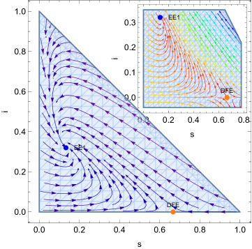
Figure 4: Stream plots of $(s,i)$ for the scaled model (2.7) illustrating the case when $\gamma_{s}$ is less than the critical vaccination $\gamma_{s}^{*}$ defined in (3.2), EE1 is a stable equilibrium point, DFE is a (boundary) saddle point, and EE2 is outside the domain.

3.1 Global stability of the disease free equilibrium

Proposition 3.

If $\mathcal{R}_{0}<1$ and DFE is the unique equilibrium point, then it is globally asymptotically stable in the invariant set $\mathcal{D}$.

Proof: Each solution starting in $\mathcal{D}$ is obviously bounded so its $\omega$-limit set is not empty. The Poincare-Bendixon Theorem implies that this is the unique equilibrium point DFE, since else it would be a closed orbit ( see HS (74)) and one may check similarly as in (DvdD, 93, Thm 3.1) that there exist no periodic orbits. $\blacksquare$

Since the explicit conditions for the uniqueness of the equilibrium point are pretty complicated, we prefer to give them only in a particular case, in section 5.

For the general case, we may find a simple criteria if we weaken the concept of global stability of the disease free equilibrium as follows

Proposition 4.

If

$$\max[\beta_{r}+\nu_{r},\beta,\Lambda+\gamma+\nu_{i}]=\Lambda+\gamma+\nu_{i},$$

then the DFE is “strongly globally stable”, in the sense that the function $L(\;\mathsf{s},\;\mathsf{i})=\;\mathsf{i}$ is Lyapunov over the invariant region $\mathcal{D}:=\left\{(\;\mathsf{s},\;\mathsf{i})\in\mathbb{R}_{+}^{2}:\;0\leq\;\mathsf{s}+\;\mathsf{i}\leq 1\right\}.$

Remark 18.

In lay terms, we may say that “the epidemics never picks up” in this case.

Proof: The non-negative function $L(\;\mathsf{s},\;\mathsf{i})=\;\mathsf{i}$, with $L(1,0)=0,$ is Lyapunov (i.e. the epidemics may never increase) iff

$$L^{\prime}(\;\mathsf{s},\;\mathsf{i})=\;\mathsf{i}^{\prime}\leq 0\Leftrightarrow s(\beta-\beta_{r}-\nu_{r})+(\nu_{i}-\nu_{r}-\beta_{r})i+\beta_{r}+\nu_{r}-\Lambda-\gamma-\nu_{i}\leq 0.$$

The maximimization of $\;\mathsf{i}^{\prime}$ reduces thus to a simple linear programming problem. Thus, there must exist an extremal point of $\mathcal{D}$ where the maximum is attained, and

$$\max_{(s,i)\in\mathcal{D}}s(\beta-\beta_{r}-\nu_{r})+(\nu_{i}-\nu_{r}-\beta_{r})i+\beta_{r}+\nu_{r}-\Lambda-\gamma-\nu_{i}=$$

$$\max[\beta_{r}+\nu_{r}-\Lambda-\gamma-\nu_{i},\beta-\Lambda-\gamma-\nu_{i},-\Lambda-\gamma]\leq 0,$$

provided that

$$\beta_{r}+\nu_{r}\leq\Lambda+\gamma+\nu_{i},{\mathcal{R}}_{0}<1\Leftrightarrow\max[\beta_{r}+\nu_{r},\beta,\Lambda+\gamma+\nu_{i}]=\Lambda+\gamma+\nu_{i}.$$ (3.6)

$\blacksquare$

4 The endemic equilibria

The endemic equilibrium set may be obtained algebraically by solving one of the variables from $\;\mathsf{i}^{\prime}/\;\mathsf{i}=0$ in (2.8), and plugging into the other equation. Eliminating $\;\mathsf{s}$ using

$$s=1-i+\frac{i(\nu_{i}-\beta)+\beta-\left(\Lambda+\gamma+\nu_{i}\right)}{-\beta+\beta_{r}+\nu_{r}},\beta\neq\beta_{r}+\nu_{r},$$

yields a quadratic equation $Ai^{2}+Bi+C=0$ where $A=\left(\beta-\beta_{r}\right)\left(\beta-\nu_{i}\right)\left(\beta_{r}+\nu_{r}-\nu_{i}\right),$ and the other coefficients are very complicated.

Thus, in the complex plane, $i^{(EE)}_{1,2}=\frac{-B\pm\sqrt{\Delta}}{2A}.$ Since locating analytically the endemic points requires considerable effort, we will restrict starting with the next section to the case $\nu_{r}=0$.

Remark 19.

We note however already that:

1. The equation is quadratic iff $\beta\neq\beta_{r},\beta\neq\nu_{i}$ and $\beta_{r}+\nu_{r}\neq\nu_{i}$. We will exclude at first these particular cases, but note that they suggest that different regimes occur when the respective thresholds are crossed – this will be further explained below.

2. Locating the endemic points may be achieved geometrically by studying the intersection of the vertical and horizontal isoclines:

   1. the $i^{\prime}=0$ isocline is given by $i=0$ and by the herd immunity line

      $$s\left(\beta-\beta_{r}-\nu_{r}\right)+i(\nu_{i}-\beta_{r}-\nu_{r})=\Lambda+\gamma+\nu_{i}-\beta_{r}-\nu_{r},$$ (4.1)

      with slope $\frac{\beta-\beta_{r}-\nu_{r}}{\beta_{r}+\nu_{r}-\nu_{i}}$.

   2. the $s^{\prime}=0$ isocline is

      $$\frac{\nu_{r}}{\Lambda+\gamma_{r}+\gamma_{s}}s^{2}+is\frac{\beta-\nu_{i}+\nu_{r}}{\Lambda+\gamma_{r}+\gamma_{s}}+s+i\frac{\gamma_{r}}{\Lambda+\gamma_{r}+\gamma_{s}}-\frac{\Lambda+\gamma_{r}}{\Lambda+\gamma_{r}+\gamma_{s}}=0,$$ (4.2)

      which is a hyperbola.

      This passes by definition through the DFE, and intersects therefore necessarily the domain when

      $$s_{dfe}<1\Leftrightarrow\gamma_{s}>0.$$

5 The case $\nu_{r}=0,\gamma_{s}>0$

Getting sharper stability results beyond the weak ${\mathcal{R}}_{0}$ alternative requires locating the endemic points, and this seems quite difficult in general. Therefore, we will restrict from now on to the case $\nu_{r}=0$, which avoids the necessity of handling the complications arising from the square root formula of $s_{dfe}$. The case $\gamma_{s}=0$, essentially covered in (DvdD, 93, Sec. 4), requires special treatment – see Section 6.

The quadratic equation $Ai^{2}+Bi+C=0$ has coefficients

$$\begin{cases}C=-\left(\gamma+\nu_{i}+\Lambda\right)\left(\Lambda+\gamma_{r}+\gamma_{s}\right)+\beta\left(\Lambda+\gamma_{r}\right)+\beta_{r}\gamma_{s}\\ B=\beta\left(-\gamma-\nu_{i}-\Lambda+\beta_{r}-\gamma_{r}\right)-\beta_{r}\left(\nu_{i}+\Lambda+\gamma_{s}\right)+\nu_{i}\left(\gamma+\nu_{i}+2\Lambda+\gamma_{r}+\gamma_{s}\right)\\ A=\left(\beta-\nu_{i}\right)\left(\nu_{i}-\beta_{r}\right)\end{cases}.$$ (5.1)

The endemic points are still complicated:

$$EE_{1,2}=\begin{cases}s=\frac{\beta\left(\gamma+\nu_{i}+\Lambda-\beta_{r}-\gamma_{r}\right)-\nu_{i}\left(\gamma+\nu_{i}-\beta_{r}-\gamma_{r}-\gamma_{s}\right)-\beta_{r}\left(\Lambda+\gamma_{s}\right)\pm\sqrt{\Delta}}{2\left(\beta-\beta_{r}\right)\left(\beta-\nu_{i}\right)}\\ i=\frac{\beta\gamma+\beta\Lambda+\beta\nu_{i}-\gamma\nu_{i}-2\Lambda\nu_{i}-\nu_{i}^{2}+\nu_{i}\beta_{r}+\Lambda\beta_{r}-\beta\beta_{r}\mp\sqrt{\Delta}}{2\left(\nu_{i}-\beta\right)\left(\beta_{r}-\nu_{i}\right)}\end{cases},$$

where

$$\Delta=4\left(\beta-\beta_{r}\right)\left(\beta-\nu_{i}\right)\left(\Lambda\left(-\nu_{i}+\beta_{r}+\nu_{r}\right)+(\gamma+\mu)\gamma_{r}\right)$$ (5.2)

$$+\left(\beta\left(-\gamma-\nu_{i}-\mu+\beta_{r}+\gamma_{r}+\nu_{r}\right)+\beta_{r}\left(-\nu_{i}+\mu+\gamma_{s}\right)+\nu_{i}\left(\gamma+\nu_{i}-\gamma_{r}-\gamma_{s}\right)-\nu_{r}\left(\gamma+\nu_{i}-\gamma_{s}\right)\right){}^{2}.$$

By solving $C=0$, we may compute however an important critical value for $\beta$,

$$\beta_{*}=\frac{\left(\gamma+\nu_{i}+\Lambda\right)\left(\Lambda+\gamma_{r}+\gamma_{s}\right)-\beta_{r}\gamma_{s}}{\Lambda+\gamma_{r}}$$ (5.3)

above which one (the higher) of the endemic points crosses above the $i=0$ axis, entering therefore $\mathcal{D}$ (equivalently, ${\mathcal{R}}_{0}$ become larger than $1$).

Locating the endemic points may be attempted algebraically –see Lemma 2 in the Appendix seemed quite difficult.

We resorted therefore to a geometric study of the isoclines in Theorem 5, attempting to explain geometrically all the possible cases. For example, the case ${\mathcal{R}}_{0}>1$ turned out equivalent to the unicity of the endemic point, and to the fact that the immunity line intersection with the domain lie on both sides of the $s^{\prime}=0$ isocline.

Remark 20.

Since the number of crossing points must be odd on one hand, and less than two on the other, identifying such a crossing is equivalent to the uniqueness of the endemic point.

We turn now to listing some elementary geometric facts, in particular the coordinates of various intersections points.

1. When $\nu_{i}\neq\beta$, the $s^{\prime}=0$ isocline becomes the hyperbola

   $$s_{dfe}=is\frac{\beta-\nu_{i}}{\Lambda+\gamma_{r}+\gamma_{s}}+\frac{\gamma_{r}}{\Lambda+\gamma_{r}+\gamma_{s}}i+s$$

   $$=i\frac{\beta-\nu_{i}}{\Lambda+\gamma_{r}+\gamma_{s}}\left(s+\frac{\gamma_{r}}{\beta-\nu_{i}}\right)+s+\frac{\gamma_{r}}{\beta-\nu_{i}}-\frac{\gamma_{r}}{\beta-\nu_{i}}$$

   $$\Leftrightarrow\left(i\frac{\beta-\nu_{i}}{\Lambda+\gamma_{r}+\gamma_{s}}+1\right)\left(s+\frac{\gamma_{r}}{\beta-\nu_{i}}\right)=s_{dfe}+\frac{\gamma_{r}}{\beta-\nu_{i}},$$

   with asymptotes $s=\frac{\gamma_{r}}{\nu_{i}-\beta},i=\frac{\Lambda+\gamma_{r}+\gamma_{s}}{\nu_{i}-\beta}$. Note that the center is in the first quadrant when $\beta<\nu_{i}$ and in the third quadrant otherwise, and that the intersection $E$ with the line $s=0$ has $i_{E}=1+\frac{\Lambda}{\gamma_{r}}$, outside $\mathcal{D}$. Also important will be the convexity of the branch which intersects $\mathcal{D}$. From

   $$i^{\prime\prime}(s_{dfe})=2\frac{s_{dfe}+k}{(s+k)^{3}}\frac{\Lambda+\gamma_{r}+\gamma_{s}}{\beta-\nu_{i}},k=\frac{\gamma_{r}}{\beta-\nu_{i}},$$

   we find that our branch is convex when $\beta>\nu_{i}$ and concave otherwise. The equality case $\nu_{i}=\beta$ is analyzed in the following remark.

   Remark 21.

   When $\nu_{i}=\beta$, the $s^{\prime}=0$ hyperbola degenerates into a line $s(\Lambda+\gamma_{r})+i\gamma_{r}-\gamma_{r}-\Lambda=0$. The intersection of the two lines gives a unique endemic point $EE=\left(\frac{(\gamma+\Lambda)\gamma_{r}}{\Lambda\left(\beta_{r}-\nu_{i}\right)}+1,\frac{(\gamma+\Lambda)\left(\Lambda+\gamma_{r}\right)}{\Lambda\left(\nu_{i}-\beta_{r}\right)}\right)$ which never belongs to the feasible region. Indeed $i_{ee}>0$ if and only if $\nu_{i}>\beta_{r}$, and this implies further

   $$s_{ee}+i_{ee}=1+\frac{(\gamma+\Lambda)\Lambda}{\Lambda(\nu_{i}-\beta_{r})}>1\Longrightarrow EE\notin\mathcal{D}.$$

2. A crucial role in the analysis is played by the point where the immunity line intersects $i=0$, given by $B(\frac{\Lambda+\nu_{i}+\gamma-\beta_{r}}{\beta-\beta_{r}},0),\beta_{r}\neq\beta$ (when $\beta_{r}=\beta$, $B$ goes to $\infty$). This point satisfies:

   $$\begin{cases}s_{B}<0&\text{if }\Lambda+\nu_{i}+\gamma<\beta_{r}<\beta,\text{ or }\beta<\beta_{r}<\Lambda+\nu_{i}+\gamma\\ s_{B}\in[0,1]&\text{if }\beta\leq\Lambda+\nu_{i}+\gamma<\beta_{r},\text{ or }\beta_{r}<\Lambda+\nu_{i}+\gamma<\beta\\ s_{B}>1&\text{if }\beta_{r}<\beta<\Lambda+\nu_{i}+\gamma\text{ or }\Lambda+\nu_{i}+\gamma<\beta<\beta_{r}\end{cases}.$$ (5.4)

   The six cases listed above are the basis of our geometric analysis provided in Theorem 5.

   Remark 22.

   $s_{B}$ coincides with $s_{dfe}$ iff $\gamma_{s}=\gamma_{s}^{*}$, which fits with the fact that $\gamma_{s}^{*}\in(0,1)$ iff one of these two cases occurs – recall Remark 16.

3. Another important point is the point $A$ where the immunity line (4.1) intersects $i=1-s$, with coordinates

   $$(s_{A},i_{A})=\left(\frac{\gamma+\Lambda}{\beta-\nu_{i}},\frac{\beta-\left(\gamma+\nu_{i}+\Lambda\right)}{\beta-\nu_{i}}\right).$$ (5.5)

   It is easy to show that $A\in\mathcal{D}$ iff $\beta>\Lambda+\nu_{i}+\gamma$, that it moves then to the fourth quadrant when $\Lambda+\nu_{i}+\gamma\geq\beta>\nu_{i}$, and that it jumps from the fourth to the second quadrant when $\beta$ decreases below the threshold $\nu_{i}$.

4. The point where the immunity line intersects $s=0$ is $C(0,1+\frac{\gamma+\Lambda}{\nu_{i}-\beta_{r}}).$ This is negative when $\nu_{i}<\beta_{r}<\Lambda+\gamma+\nu_{i}$, in the domain when $\beta_{r}\geq\Lambda+\gamma+\nu_{i}$, and bigger than $1$ when $\beta_{r}\leq\nu_{i}$. More precisely,

   $$C=\frac{\Lambda+\gamma+\nu_{i}-\beta_{r}}{\nu_{i}-\beta_{r}}\text{ satisfies\ }\begin{cases}i_{C}\leq 0&\text{if }\nu_{i}<\beta_{r}<\Lambda+\nu_{i}+\gamma\\ i_{C}\in[0,1]&\text{if }\beta_{r}\geq\Lambda+\nu_{i}+\gamma\\ i_{C}>1&\text{if }\beta_{r}<\nu_{i}\end{cases}.$$

5. The unique point $D$ where the hyperbola intersects $\;\mathsf{s}+\;\mathsf{i}=1$ within the domain has coordinates

   $$\begin{cases}s_{D}=\frac{1}{2}+\frac{\Lambda+\gamma_{s}-\sqrt{4\Lambda\left(\nu_{i}-\beta\right)+\left(\beta-\nu_{i}+\Lambda+\gamma_{s}\right){}^{2}}}{2\left(\beta-\nu_{i}\right)}\\ i_{D}=\frac{1}{2}+\frac{-\Lambda-\gamma_{s}+\sqrt{4\Lambda\left(\nu_{i}-\beta\right)+\left(\beta-\nu_{i}+\Lambda+\gamma_{s}\right){}^{2}}}{2\left(\beta-\nu_{i}\right)}\end{cases}.$$ (5.6)

Remark 23.

When $\beta=\beta_{r}$, the slope $\frac{\beta-\beta_{r}}{\beta_{r}-\nu_{i}}$ of the immunity line becomes $0$ and $i_{C}=i_{A}=\frac{\beta-\left(\gamma+\nu_{i}+\Lambda\right)}{\beta-\nu_{i}}=\frac{1}{\gamma+\nu_{i}+\Lambda}\frac{{\mathcal{R}}_{0}-1}{\beta-\nu_{i}}.$ The dynamical system admits a unique endemic point and a unique EE given by

$$EE=\left(\frac{\Lambda\left(\beta-\nu_{i}+\gamma_{r}\right)+\gamma\gamma_{r}}{\left(\beta-\nu_{i}\right)\left(\beta-\gamma-\nu_{i}+\gamma_{r}+\gamma_{s}\right)},\frac{\beta-\Lambda+\gamma+\nu_{i}}{\beta-\nu_{i}}\right),$$

which may be checked to belong to the feasible region iff

$$\mathcal{R}=\frac{\beta}{\Lambda+\gamma+\nu_{i}}>1.$$

Indeed, $i_{ee}>0$ requires either $\beta<\nu_{i}$, which leads subsequently to a contradiction, or $\beta>\Lambda+\gamma+\nu_{i}$, which may be shown to imply $s>0,s+i<1$. The stability analysis of this case is elementary and left to the reader.

The formula (5.4) and the subsequent Remark 22 suggest splitting the analysis according to the order of the three quantities $\beta,\Lambda+\gamma+\nu_{i},\beta_{r}$ and on the orders of $\gamma_{s},\gamma_{s}^{*}=\left(\Lambda+\gamma_{r}\right)\frac{\beta-\left(\Lambda+\gamma+\nu_{i}\right)}{\Lambda+\gamma+\nu_{i}-\beta_{r}}$ and of $(\nu_{i},\beta)$. We end up with ten cases, nine of which are fully resolved in Theorem 5, and one of which is left partly open. Note that, as proved in the Appendix, these ten cases form a disjoint decomposition of the parameter space, if only strict inequalities are allowed.

Before stating Theorem 5, we provide graphical illustrations of the 10 cases.

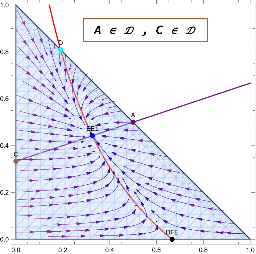
(a) $\beta=5>\beta_{r}=4>3=\Lambda+\gamma+\nu_{i}=1+1+1,\gamma_{r}=1,\gamma_{s}=1>\gamma_{s}^{*}\Leftrightarrow s_{B}>1,\beta>\beta_{r}>\gamma+\nu_{i}+\Lambda,$.

(b) $\beta_{r}=4>\beta=3.5>0.21=\Lambda+\gamma+\nu_{i}=1+1+0.1,\gamma_{r}=1/6,\gamma_{s}=0.01.$

(c) $B,A\in\mathcal{D}$, with $\beta=0.3>0.21=\Lambda+\gamma+\nu_{i}=0.01+0.05+0.15>\beta_{r}=0.1,\gamma_{r}=1/26,\gamma_{s}.=.015<\gamma_{s}^{*}\Leftrightarrow s_{B}<s_{dfe}$.

(d) $B,C\in\mathcal{D}$, with ${\mathcal{R}}_{0}=1.04762>1,\beta=2<\Lambda+\gamma+\nu_{i}=1+1+1=3<\beta_{r}=4,\gamma_{r}=1/2,\gamma_{s}=2>\gamma_{s}^{*}\Leftrightarrow s_{B}>s_{dfe}$.

Figure 5: Stream plots of $(\;\mathsf{s},\;\mathsf{i})$ when $\gamma_{s}>0$, in four cases when ${\mathcal{R}}_{0}>1$. The DFE is a saddle point and EE is a stable sink.

Figure 7: Diagram bifurcation with respect to $\beta$, in the case $\max[\Lambda+\gamma+\nu_{i},\beta_{r}^{(+)}]<\beta_{r}$. For $\beta<\nu_{i}$ we are in the case of Fig. 4(b) (Thm. 5.2.b)), with the immunity line to the left of the hyperbola, and no endemic points. The same situation occurs for $\nu_{i}<\beta<\beta_{2}$, where $\beta_{2}$ is the largest root of $\Delta(\beta)=0$, except that the hyperbola changes to convex – see Fig. 4(c) (Thm. 5.2.c)(i)). After $\beta_{2}$ two endemic points emerge – see Fig. 4(d) (Thm. 5.2.c)(ii)). The lower endemic point exits through the boundary $i=0$ at $\beta*$, defined in (5.3), after which the remaining endemic point remains the only stable point.

Theorem 5.

Suppose $\nu_{r}=0$, and that neither two of the three parameters $\beta,\beta_{r},\nu_{i}$ coincide. Then, one of the following cases must arise:

1. ${\mathcal{R}}_{0}>1\Leftrightarrow$ precisely one endemic point lies in $\mathcal{D}$, which may occur in one of the following four ways:

   1. $AC\in\mathcal{D}$ crosses the hyperbola with positive slope $\Lambda+\gamma+\nu_{i}\leq\beta_{r}<\beta$ –see Figure 3(a);

   2. $AC\in\mathcal{D}$ crosses the hyperbola with negative slope $\Lambda+\gamma+\nu_{i}\leq\beta<\beta_{r}$ –see Figure 3(b);

   3. $\beta_{r}\leq\Lambda+\gamma+\nu_{i}\leq\beta,\gamma_{s}<\gamma_{s}^{*}\Leftrightarrow$ $BA\in\mathcal{D}$ crosses the hyperbola – Fig. 3(c);

   4. $\beta\leq\Lambda+\gamma+\nu_{i}\leq\beta_{r},\gamma_{s}\geq\gamma_{s}^{*}\Leftrightarrow$ $BC\in\mathcal{D}$ crosses the hyperbola – Fig. 3(d).

   In all these cases, the endemic point is a sink and DFE is a saddle point.

2. ${\mathcal{R}}_{0}\leq 1$ is the union of the following six cases (similar to the above, but taking also into account the convexity of the hyperbola branch, in some cases):

   1. $$\beta_{r}<\Lambda+\gamma+\nu_{i}<\beta,\nu_{i}<\beta,$$

      when both the points $A,B$ lie to the right of a convex hyperbola branch, and the isoclines do not intersect in $\mathcal{D}$–see Figure 4(a).

   2. $$\beta<\nu_{i}<\Lambda+\gamma+\nu_{i}<\beta_{r},$$

      when both the points $C,B$ lie to the left of a concave hyperbola branch, and the isoclines do not intersect in $\mathcal{D}$–see Figure 4(b).

   3. When both the points $C,B$ lie to the left of a convex hyperbola branch, we have two subcases:

      1. When

         $$\nu_{i}<\beta<\Lambda+\gamma+\nu_{i}<\beta_{r},\gamma_{s}<\gamma_{s}^{*},\Delta<0,$$

         the isoclines intersect $\mathcal{D}$, but do not intersect each other –see Figure 4(c).

      2. The isoclines intersect in $\mathcal{D}$, yielding two endemic points –see Figure 4(d). Necessary conditions for this are

         $$\nu_{i}<\beta{<\Lambda+\gamma+\nu_{i}<\beta_{r}},\gamma_{s}<\gamma_{s}^{*},\Delta\geq 0,$$

         and we conjecture that the necessary and sufficient conditions are obtained by adding $\beta_{r}\geq\beta_{r}^{(+)}$, where $\beta_{r}^{(+)}$ is defined in (5.8).

         In this case, the DFE is one of two sink points, whose attraction domains are separated by the separatrices of the third fixed saddle point.

   4. The $i^{\prime}/i=0$ isocline does not intersect the interior of $\mathcal{D}$ in the following two cases:

      1. $\beta\leq\beta_{r}\leq\Lambda+\gamma+\nu_{i}$, with hyperbole concave – see figure 5(a)– or convex, according to whether $\beta>\nu_{i}$ or not;

      2. $\beta_{r}<\beta\leq\Lambda+\gamma+\nu_{i}$, with hyperbole convex – see figure 5(b)– or convave, according to whether $\beta<\nu_{i}$ or not;

3. In all the cases when the DFE is the unique fixed point within the domain, it is a globally stable sink.

Proof:

1. As noted already, $\beta>\Lambda+\gamma+\nu_{i}$ is equivalent to fact that the point $A=(\frac{\gamma+\Lambda}{\beta-\nu_{i}},\frac{\beta-\nu_{i}-\gamma-\Lambda}{\beta-\nu_{i}})$ lies in $\mathcal{D}$, which applies in the cases 1.(a), 1.(b), 1.(c). Furthermore, we may check that in this case the point $A$ is always to the right (above) the hyperbola, i.e.

   $$s_{D}=\frac{1}{2}+\frac{\Lambda+\gamma_{s}-\sqrt{4\Lambda\left(\nu_{i}-\beta\right)+\left(\beta-\nu_{i}+\Lambda+\gamma_{s}\right){}^{2}}}{2\left(\beta-\nu_{i}\right)}<\frac{\gamma+\Lambda}{\beta-\nu_{i}}=s_{A}.$$

   To conclude the existence of a unique endemic point, it is enough then to find in these three cases a point of the immunity line below the hyperbola. Referring to Figures 3, we see that the following cases may arise:

   1. $AC\in\mathcal{D}$ crosses the hyperbola, and $s_{B}<0$. We must then be in the case $\Lambda+\gamma+\nu_{i}<\beta_{r}<\beta$, which implies $\beta_{r}\geq\Lambda+\nu_{i}+\gamma$, and so $C\in\mathcal{D}$ is below the hyperbola –see Figure 3(a).

   2. $AC\in\mathcal{D}$ crosses the hyperbola, and $s_{B}\geq 1$. We must then be in the case $\Lambda+\gamma+\nu_{i}<\beta<\beta_{r}$, which implies again $\beta_{r}\geq\Lambda+\nu_{i}+\gamma$, and so $C\in\mathcal{D}$ is again below the hyperbola – see Figure 3(b).

   3. $BA\in\mathcal{D}$ crosses the hyperbola when ${\mathcal{R}}_{0}>1,\beta>\Lambda+\gamma+\nu_{i}>\beta_{r},s_{B}\leq s_{dfe}\Leftrightarrow\gamma_{s}\leq\gamma_{s}^{*}$, since $B$ is below the hyperbola –see Figure 3(c).

   4. $BC\in\mathcal{D}$ crosses the hyperbola (and $A\notin\mathcal{D}$) when ${\mathcal{R}}_{0}>1,\beta_{r}>\Lambda+\gamma+\nu_{i}>\beta,s_{B}>s_{dfe}\Leftrightarrow\gamma_{s}\geq\gamma_{s}^{*}$, since $B$ is below the hyperbola –see Figure 3(d).

2. We turn now to the case ${\mathcal{R}}_{0}\leq 1$, when the point $A$ lies in the fourth quadrant if $\nu_{i}<\beta$, and in the second quadrant otherwise.

   1. In this case $s_{B}>s_{dfe},s_{A}>s_{D}$. Since the immunity line is to the right of a convex hyperbola branch, it is clear geometrically that they cannot intersect within the domain – see Figure 4(a).

   2. Similarly, the end points in $\mathcal{D}$ of the immunity line are to the left of a concave hyperbola branch, and so they cannot intersect within the domain – see Figure 4(b).

   3. For two endemic points to exist, it is necessary that $s_{B}=\frac{\Lambda+\nu_{i}+\gamma-\beta_{r}}{\beta-\beta_{r}}\in(0,s_{dfe})$, which requires that

      $$\beta\leq\Lambda+\gamma+\nu_{i}\leq\beta_{r},$$

      and this implies that the other intercept $C=(0,\frac{\Lambda+\gamma+\nu_{i}-\beta_{r}}{\nu_{i}-\beta_{r}})$ is also in $\mathcal{D}$.

      The $i^{\prime}/i=0$ isocline intersects then $\mathcal{D}$, and may also intersect the hyperbola, when the discriminant

      $$\Delta=\left(\nu_{i}(\nu_{i}-\beta_{r}+\gamma-\gamma_{r}-\gamma_{s})+\beta_{r}(\gamma_{s}+\Lambda)+\beta(\beta_{r}-\gamma+\gamma_{r}-\Lambda-\nu_{i})\right)^{2}$$

      $$+4(\beta-\beta_{r})(\beta-\nu_{i})(\gamma\gamma_{r}+\Lambda(\beta_{r}+\gamma_{r}-\nu_{i}))$$ (5.7)

      satisfies  $\Delta\geq 0$.

      The inequality $\Delta>0$ is quadratic in $\beta_{r}$ and maybe rewritten as

      $$\beta_{r}+\Lambda+\gamma_{r}-\nu_{i}+\frac{\Lambda\left(\Lambda+\gamma_{r}\right)}{\beta-\nu_{i}-\Lambda}-\frac{\gamma\left(\beta-\nu_{i}\right)\left(\beta-\nu_{i}+\Lambda+2\gamma_{r}\right)}{\left(\beta-\nu_{i}-\Lambda\right){}^{2}}\notin[-\mathcal{L},\mathcal{L}]$$

      $$\mathcal{L}=2\frac{\sqrt{\gamma\left(\Lambda+\gamma_{r}\right)\left(\beta-\nu_{i}\right){}^{2}\left(\beta-\nu_{i}+\gamma_{r}\right)\left(\Lambda+\gamma+\nu_{i}-\beta\right)}}{\left(\beta-\nu_{i}-\Lambda+\gamma_{s}\right){}^{2}+4\Lambda\gamma_{s}}$$ (5.8)

      (note that $\mathcal{L}>0$ when $\mathcal{R}<1,\nu_{i}<\beta)$.

      We conjecture based on numerical evidence that the two endemic points belong to $\mathcal{D}$ only when $\beta_{r}$ is larger than the largest root $\beta_{r}^{(+)}$ of $\Delta=0$, defined implicitly in (5.8)

   4. In the last case we must show that the $i^{\prime}/i=0$ isocline does not intersect the interior of $\mathcal{D}$. Equivalently, we must show that in each of the two subcases

      $$\begin{cases}\beta<\beta_{r}\leq\Lambda+\gamma+\nu_{i}\\ \beta_{r}\leq\beta\leq\Lambda+\gamma+\nu_{i}\end{cases}$$

      none of the points $A,B,C$ belongs to $\mathcal{D}$. This is a tedious computation, not reproduced here. For a quick check, we offer a Mathematica file on our website (we rely mostly on FindInstance with empty output to show that certain cases do not exist, and on the command Reduce to decompose other cases into subcases).

$\blacksquare$

6 The boundary case $\gamma_{s}=\nu_{r}=0$

The case $\gamma_{s}=\nu_{r}=0$, generalizes on the particular case $\gamma_{s}=\nu_{r}=0=\gamma_{r}$, which was called SIRI model in (DvdD, 93, Sec. 4).

Note first that in this case $s_{dfe}=1$. It follows that  the 4, 5 cases (1(d) and 2(a)) may not arise,and the case 6 (2(b)) becomes degenerate since $s_{dfe}=1$. It becomes now possible that the hyperbola does not intersect the domain. This is equivalent to its slope at the DFE $i^{\prime}(s_{dfe})=-\frac{\Lambda+\gamma_{r}}{\beta-\nu_{i}+\gamma_{r}}$ being either positive or less than $-1$, and further equivalent to

$$\beta\leq\Lambda+\nu_{i}.$$

This further implies $\mathcal{R}_{0}<1$, and, together with the absence of endemic points and of periodic solutions, leads to the fact that the DFE is the global attractor.

After having dealt with this case, which includes also the concave case $\beta>\nu_{i}$, one may restrict to the case when the hyperbola does intersect the domain, which is equivalent to its slope at the DFE being such that

$$-1<i^{\prime}(s_{dfe})<0\Leftrightarrow\beta>\Lambda+\nu_{i}$$

(note this implies that its center is in the third quadrant).

The proof becomes simpler than in the previous section. For example, the point $D$ of intersection of the hyperbola with $i=1-s$ satisfies

$$s_{D}=\frac{\Lambda}{\beta-\nu_{i}}{\in(0,1)},$$

and hence belongs to $\mathcal{D}$.

The roots of $\Delta=0$ simplify now to:

$$\beta_{r}^{(\pm)}:=\nu_{i}-\Lambda-\gamma_{r}-\frac{\Lambda\left(\Lambda+\gamma_{r}\right)}{\beta-\nu_{i}-\Lambda}+\frac{\gamma\left(\beta-\nu_{i}\right)\left(\beta-\nu_{i}+\Lambda+2\gamma_{r}\right)}{\left(\beta-\nu_{i}-\Lambda\right){}^{2}}\pm\mathcal{L},$$ (6.1)

$$\mathcal{L}=2\frac{\sqrt{\gamma\left(\Lambda+\gamma_{r}\right)\left(\beta-\nu_{i}\right){}^{2}\left(\beta-\nu_{i}+\gamma_{r}\right)\left(\Lambda+\gamma+\nu_{i}-\beta\right)}}{\left(-\beta+\nu_{i}+\Lambda\right){}^{2}}.$$

7 The classic/pedagogical SIR/V+S model

The pedagogical model is defined as follows:

$$\;\mathsf{s}^{\prime}(t) =\Lambda-\beta\;\mathsf{s}(t)\;\mathsf{i}(t)+\gamma_{r}\;\mathsf{r}(t)-{(\gamma_{s}+\mu)}\;\mathsf{s}(t),$$

$$\;\mathsf{i}^{\prime}(t) =\;\mathsf{i}(t)\left[\beta\;\mathsf{s}(t)+\beta_{r}\;\mathsf{r}(t)-\left(\gamma+{\nu_{i}+\mu}\right)\right],$$

$$\;\mathsf{r}^{\prime}(t) =\gamma\;\mathsf{i}(t)+\gamma_{s}\;\mathsf{s}(t)-{(\gamma_{r}+\mu+\nu_{r})}\;\mathsf{r}(t)-\beta_{r}\;\mathsf{r}(t)\;\mathsf{i}(t).$$ (7.1)

The following properties hold:

1. The region

   $$\mathcal{D}=\{(\;\mathsf{s},\;\mathsf{i},N)\in\mathbb{R}_{{+}}^{3},\;\mathsf{s}+\;\mathsf{i}\leq N\leq\Lambda/\mu\}$$ (7.2)

   may be shown to   be positively invariant with respect to (7); therefore, this region must include an attractor set MLH (92); VDL (09).

2. The DFE equilibrium point of the pedagogic system is obtained plugging $i_{dfe}=0$ in (7). Solving with respect to $(\;\mathsf{s},\;\mathsf{r})$ the remaining first and third equation

   $$\begin{cases}0=\Lambda-(\gamma_{s}+\mu)\;\mathsf{s}+\gamma_{r}\;\mathsf{r},\\ 0=\gamma_{s}\;\mathsf{s}-(\gamma_{r}+\mu+\nu_{r})\;\mathsf{r},\end{cases}$$

   yields

   $$X^{(DFE)}=\left(\frac{\Lambda\left(\mu+\gamma_{r}+\nu_{r}\right)}{\mu\gamma_{r}+\left(\mu+\nu_{r}\right)\left(\mu+\gamma_{s}\right)},0,\frac{\Lambda\gamma_{s}}{\mu\gamma_{r}+\left(\mu+\nu_{r}\right)\left(\mu+\gamma_{s}\right)}\right).$$ (7.3)

   In particular, the DFE for the FA model is obtained by substituting $\Lambda=\mu$ in (7.3):

   $$X^{(DFE)}=\left(\frac{\Lambda\left(\Lambda+\gamma_{r}+\nu_{r}\right)}{\Lambda\gamma_{r}+\left(\Lambda+\nu_{r}\right)\left(\Lambda+\gamma_{s}\right)},0,\frac{\Lambda\gamma_{s}}{\Lambda\gamma_{r}+\left(\Lambda+\nu_{r}\right)\left(\Lambda+\gamma_{s}\right)}\right).$$ (7.4)

   Note the relation $\nu_{r}\gamma_{s}=0\Longrightarrow i_{dfe}+r_{dfe}+s_{dfe}=1.$

3. When $\beta_{r}>0$ there may be two endemic equilibrium points (we omit their complicated expressions), but when $\beta_{r}=0$ there is a unique FA EE, obtained by plugging

   $$s=\frac{1}{\mathcal{R}}=\frac{\gamma+\Lambda+\nu_{i}}{\beta}$$

   in the first and third equation, and solving the linear system

   $$\begin{cases}\Lambda+\gamma_{r}\;\mathsf{r}(t)-\beta\;\mathsf{i}/\mathcal{R}-(\gamma_{s}+\Lambda)/\mathcal{R}=0,\\ \gamma\;\mathsf{i}+\gamma_{s}/\mathcal{R}-(\gamma_{r}+\Lambda+\nu_{r})\;\mathsf{r}=0\end{cases}.$$ (7.5)

   This yields $X^{(EE)}=$

   $$\left(\frac{1}{\mathcal{R}},\frac{\gamma_{r}(\Lambda-\Lambda\mathcal{R})+(\Lambda+\nu_{r})(\gamma_{s}+\Lambda-\Lambda\mathcal{R})}{\gamma\gamma_{r}\mathcal{R}-\beta(\gamma_{r}+\Lambda+\nu_{r})},\frac{\gamma\mathcal{R}(\gamma_{s}+\Lambda-\Lambda\mathcal{R})-\beta\gamma_{s}}{\mathcal{R}(\gamma\gamma_{r}\mathcal{R}-\beta(\gamma_{r}+\Lambda+\nu_{r}))}\right)$$ (7.6)

   $$=\left(\frac{1}{\mathcal{R}},\frac{\mathcal{R}s_{dfe}-1}{z},\frac{\gamma\mathcal{R}(\gamma_{s}+\Lambda-\Lambda\mathcal{R})-\beta\gamma_{s}}{\mathcal{R}(\gamma\gamma_{r}\mathcal{R}-\beta(\gamma_{r}+\Lambda+\nu_{r}))}\right),$$

   where $z:=\mathcal{R}\left[\frac{\gamma_{r}(\Lambda+\nu_{i})+(\Lambda+\nu_{r})(\gamma+\Lambda+\nu_{i})}{\Lambda\gamma_{r}+\left(\Lambda+\nu_{r}\right)\left(\Lambda+\gamma_{s}\right)}\right]$.

   Note the intriguing simplification of $i^{(EE)}$, which shows that

   $$i^{(EE)}\geq 0\Leftrightarrow 1\leq\mathcal{R}s_{dfe},$$

   and it may be shown that the endemic point belongs to the domain iff $1\leq\mathcal{R}s_{dfe}$. This gives a pre-warning on the role of the parameter $\mathcal{R}s_{dfe}:=\mathcal{R}_{0}$ in the stability of the DFE.

Example 1.

In the particular case $\nu_{r}=\gamma_{r}=\gamma_{s}=0\Longrightarrow s_{dfe}=1$, we recover the SIR-FA example, for which the sharp threshold property holds (SvdD, 13, (4.1)), i.e. the disease free equilibrium is globally stable iff $\mathcal{R}_{0}=\mathcal{R}\;s_{dfe}\leq 1$.

The endemic point simplifies to

$$X^{(EE)}=\left(\frac{1}{\mathcal{R}},\frac{\Lambda}{\beta}\left(\mathcal{R}-1\right),\frac{\gamma}{\beta}\left(\mathcal{R}-1\right)\right).$$

We may observe that the endemic point $X^{(EE)}$ is positif if $\mathcal{R}>1$.

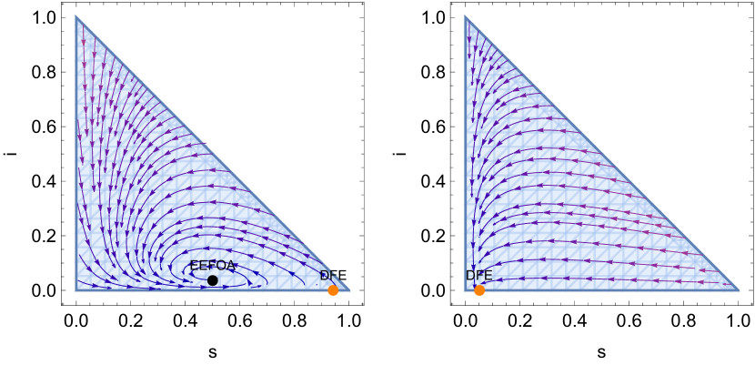
Figure 8: Stream plots of $(s,i)$ for the FA model when $\gamma_{s}\in\left\{1/100,3\right\}$ is smaller and bigger, respectively, than the critical vaccination $\gamma_{s}^{*}=0.239087$ defined in (3.3).

8 Appendix A: Auxiliary lemmas

Lemma 1.

If only strict inequalities between $\Lambda+\gamma+\nu_{i},\beta_{r}$ and $\beta$ are allowed, then the following ten cases

$$\begin{cases}\Lambda+\gamma+\nu_{i}<\beta_{r}<\beta\\ \Lambda+\gamma+\nu_{i}<\beta<\beta_{r}\\ \beta_{r}<\Lambda+\gamma+\nu_{i}<\beta,\gamma_{s}<\gamma_{s}^{*}\\ \beta<\Lambda+\gamma+\nu_{i}<\beta_{r},\gamma_{s}\geq\gamma_{s}^{*}\\ \beta_{r}<\Lambda+\gamma+\nu_{i}<\beta,\nu_{i}<\beta\\ \beta<\nu_{i}<\Lambda+\gamma+\nu_{i}<\beta_{r}\\ \nu_{i}<\beta{<\Lambda+\gamma+\nu_{i}<\beta_{r}},\gamma_{s}<\gamma_{s}^{*},\Delta<0\\ \nu_{i}<\beta{<\Lambda+\gamma+\nu_{i}<\beta_{r}},\gamma_{s}<\gamma_{s}^{*},\Delta\geq 0\\ \beta<\beta_{r}<\Lambda+\gamma+\nu_{i}\\ \beta_{r}<\beta<\Lambda+\gamma+\nu_{i}\end{cases},$$

form a disjoint decomposition of the parameter space.

Proof: We note first that in all cases where equality is allowed, the equality case may be arbitrarily assigned to any of the two cases it separates. It is enough therefore to consider only strict inequalities in this Lemma.

We want to show that the union of the ten cases equals the union of the six cases representing the possible orders of $\beta,\beta_{r},\Lambda+\gamma+\nu_{i}$, which are

$$\begin{cases}\beta>\beta_{r}>\gamma+\nu_{i}+\Lambda&1\\ \beta_{r}>\beta>\gamma+\nu_{i}+\Lambda&2\\ \beta>\gamma+\nu_{i}+\Lambda>\beta_{r}&3\\ \beta_{r}>\gamma+\nu_{i}+\Lambda>\beta&4\\ \gamma+\nu_{i}+\Lambda>\beta_{r}>\beta&5\\ \gamma+\nu_{i}+\Lambda>\beta>\beta_{r}&6\end{cases}.$$

Now the cases $1,2,$ with $\Lambda+\gamma+\nu_{i}<\min[\beta,\beta_{r}]$, and the cases $9,10,$ with $\Lambda+\gamma+\nu_{i}>\min[\beta,\beta_{e}]$ appear only once in the ten cases of theorem 5, as case 1.(a), 1(b), and 2(d)(i-ii).

Next, we may check that the union of the cases 3 and 5 (1.(c) and 2.(a) in the Theorem) form together the permutation 3. This requires checking that the other two of the four formal cases taking into account the possible orders between $\beta,\nu_{i}$ and $\gamma_{s},\gamma_{s}^{*}$ are void; the tedious verification is included in the Mathematica file available on our website.

To conclude, it remains to check that the cases 4,6,7,8 (i.e. 1.(d), 2.(b), 2.(c)(i) and 2.(c)(ii) in the Theorem) form together a partition of the permutation 4. Note first that cases 7 and 8 may be combined in $\nu_{i}<\beta<\Lambda+\gamma+\nu_{i}<\beta_{r},\gamma_{s}<\gamma_{s}^{*}$. Next, we show in the Mathematica file that the case 4 $\beta<\Lambda+\gamma+\nu_{i}<\beta_{r},\gamma_{s}\geq\gamma_{s}^{*}$ is incompatible with $\beta<\nu_{i}$, and so we can modify the case 4 to $\nu_{i}<\beta<\Lambda+\gamma+\nu_{i}<\beta_{r},\gamma_{s}\geq\gamma_{s}^{*}$. So, 4, 6 and 7-8 become

$$\begin{cases}\nu_{i}<\beta<\Lambda+\gamma+\nu_{i}<\beta_{r},\gamma_{s}\geq\gamma_{s}^{*}\\ \beta<\nu_{i}<\Lambda+\gamma+\nu_{i}<\beta_{r}\\ \nu_{i}<\beta{<\Lambda+\gamma+\nu_{i}<\beta_{r}},\gamma_{s}<\gamma_{s}^{*},\end{cases}$$

whose union is clearly the permutation 4. $\square$

Lemma 2.

A) A necessary and sufficient condition for having precisely one endemic point with $s\in(0,1)$ is $C(A+B+C)<0$, where $A,B,C$ are defined in (5.1).

B) Necessary and sufficient conditions for having precisely two endemic points with $s\in(0,1)$ are $\Delta>0$ and

$$-2<\frac{B}{A}<0<\frac{C}{A},\frac{B}{A}>-1-\frac{C}{A}.$$

Proof: The conditions for having two roots bigger than 0 are $\frac{B}{A}<0<\frac{C}{A}$, and the conditions for having two roots smaller than 1 are obtained by applying these, after substituting $y=1-x$, yielding the result. $\square$

Since expressing these simple conditions in terms of the parameters of the model turned out quite difficult, we did not finalize this approach.

9 Apendix B: A short review of deterministic epidemic models

9.1 What is a deterministic epidemic model?

To put in perspective our work, we would like to start by a definition of deterministic epidemic models, lifted from KS (08).

Definition 2.

A deterministic epidemic model is a dynamical system with two types of variables $\vec{x}(t):=(\vec{\;}\mathsf{i}(t),\vec{z}(t))\in{\mathbb{R}}_{+}^{N}$, where

1. $\vec{\;}\mathsf{i}(t)$ model the number (or density) in different compartments of infected individuals (i.e. latent, infectious, hospitalized, etc) which should ideally disappear eventually if the epidemic ever ends;

2. $\vec{z}(t)$ model numbers (or densities) in compartments of individuals who are not infected (i.e. susceptibles, immunes, recovered individuals, etc).

The system must admit an equilibrium called disease free equilibrium (DFE), and hence a “quasi-triangular” linearization the form

$$\vec{\;}\mathsf{i}^{\prime}(t) =\vec{\;}\mathsf{i}(t)A_{i,i}(\vec{x}(t)),\vec{x}(t)\in\mathcal{D}\subset{\mathbb{R}}_{+}^{N}$$ (9.1)

$$\vec{z}^{\prime}(t) =\vec{\;}\mathsf{i}(t)A_{z,i}(\vec{x}(t))+(\vec{z}(t)-\vec{z}_{dfe})A_{z,z}(\vec{x}(t)),$$

where $\mathcal{D}$ is some forward-invariant subset, where “quasi-triangular” refers to the fact that the functions $A_{i,i},A_{z,i},A_{z,z}$ depend on all the variables $\vec{x}(t)$, and where $N$ is the dimension of $\vec{x}(t)$. $\square$

As shown in KS (08), any epidemic model admitting an equilibrium point $(\vec{0},\vec{z}_{dfe})$ admits the representation (9.1), under suitable smoothness assumptions. In what follows, we will call the point $x_{dfe}=(\vec{0},\vec{z}_{dfe})$ a disease free equilibrium  (DFE).

Remark 24.

Note that the essential feature of (9.1) is the “factorization of the disease equations”. $\square$

9.2 The basic reproduction number and the next generation matrix method

One of the central objectives in mathematical epidemiology is to study the stability of DFE, i.e. the conditions which make possible eradicating the sickness. For simple models, this amounts, independently of the initial state, to verifying that a famous threshold parameter called basic reproduction number ${\mathcal{R}}_{0}$ is less than $1$ (and the fundamental problem of interest is, when ${\mathcal{R}}_{0}>1$, to offer control strategies which force the epidemic to reach the DFE).

The basic reproduction number or “net reproduction rate” ${\mathcal{R}}_{0}$ is a pillar concept in demography, branching processes and mathematical epidemiology – see the introduction of the book Bac (21).

1. The notation was first introduced by the father of mathematical demography Lotka Lot (39); Die (93). In epidemiology, the basic reproduction number models the expected number of secondary cases which one infected case would produce in a homogeneous, completely susceptible stochastic population, in the next generation. As well known in the simplest setup of branching process, having this parameter smaller than $1$ makes extinction sure. The relation to epidemiology is that an epidemics is well approximated by a branching process at its inception, a fact which goes back to Bartlett and Kendall.

2. With more infectious classes, one deals at inception with multi-class branching processes, and stability holds when the Perron-Frobenius eigenvalue of the “next generation matrix ” (NGM) of means is smaller than $1$.

3. For deterministic epidemic models, it seems at first that the basic reproduction number ${\mathcal{R}}_{0}$ is lost, since the generations disappear in this setup – but see (Bac, 21, Ch. 3), who recalls a method to introduce generations which goes back to Lotka, and which is reminiscent of the iterative Lotka-Volterra approach of solving integro-differential. At the end of the tunnel, a unified method for defining ${\mathcal{R}}_{0}$ emerged only much later, via the “next generation matrix” approach DHM (90); vdDW (02); VdDW (08); DHR (10); Per (18). The final result is that local stability of the disease free equilibrium holds iff the spectral radius of a certain matrix called “next generation matrix”, which depends only on a set of “infectious compartments” $\vec{\;}\mathsf{i}$ (which we aim to reduce to $0$), is less than one. This approach works provided that certain assumptions listed below hold .

1. The foremost assumption is that the disease-free equilibrium $(\vec{0},z_{dfe})$ is unique and locally asymptotically stable within the disease-free space $\vec{\;}\mathsf{i}=0$, meaning that all solutions of

   $$\vec{z}^{\prime}(t)=(\vec{z}(t)-\vec{z}_{dfe})A_{z,z}(\vec{0},\vec{z}(t)),\quad\vec{z}(0)=\vec{z}_{0}$$

   must approach the point $z_{dfe}$ when $t\to\infty$).

2. Other conditions are related to an “admissible splitting” as a difference of two parts $\mathcal{F},\mathcal{V}$, called respectively  “new infections”, and “transitions”

   Definition 3.

   A splitting

   $$\vec{\;}\mathsf{i}^{\prime}(t)=\mathcal{F}(\vec{\;}\mathsf{i}(t),\vec{z}(t))-\mathcal{V}(\vec{\;}\mathsf{i}(t),\vec{z}(t))$$

   will be called admissible if $\mathcal{F},\mathcal{V}$ satisfy the following conditions VdDW (08); SvdD (13):

   1. $$\begin{cases}\mathcal{F}(\vec{0},\vec{z}(t))=\mathcal{V}(\vec{0},\vec{z}(t))=0\\ \mathcal{F}(\vec{\;}\mathsf{i}(t),\vec{z}(t))\geq 0,\forall(\vec{\;}\mathsf{i}(t),\vec{z}(t))\\ \mathcal{V}_{j}(\vec{\;}\mathsf{i}(t),\vec{z}(t))\leq 0,\text{ when }\vec{\;}\mathsf{i}_{j}=0,\\ \sum_{j=1}^{n}\mathcal{V}_{j}(\vec{\;}\mathsf{i}(t),\vec{z}(t))\geq 0,\forall(\vec{\;}\mathsf{i}(t),\vec{z}(t)).\end{cases},$$ (9.2)

      where the subscript $j$ refers the $j$’th component.

   Remark 25.

   The splitting of the infectious equations has its origins in epidemiology. Mathematically, it is related to the ”splitting of Metzler matrices”– see for example  FIST (07). Note however that the splitting conditions may be satisfied for several or for no subset of compartments (see for example  the SEIT model, discussed in VdDW (08), (Mar, 15, Ch 5)). Unfortunately, for deterministic epidemic models, there is no clear-cut definition of ${\mathcal{R}}_{0}$ Rob (07); LB ; Thi (18).

3. We turn now to the last conditions, which concern the linearization of the infectious equations around the DFE. Putting $L=A_{i,i}(\vec{0},\vec{z}_{dfe})$, and letting $f$ denote the perturbation from the linearization, we may write:

   $$\vec{\;}\mathsf{i}^{\prime}(t) =\vec{\;}\mathsf{i}(t)L-f(\vec{\;}\mathsf{i}(t),\vec{z}(t))=\vec{\;}\mathsf{i}(t)(F-V)-f(\vec{\;}\mathsf{i}(t),\vec{z}(t)),$$

   $$F:=\left[\frac{\partial\mathcal{F}}{\partial\;\mathsf{i}}\right]_{x_{dfe}}V=\left[\frac{\partial\mathcal{V}}{\partial\;\mathsf{i}}\right]_{x_{dfe}},L=F-V.$$

   The “transmission and transition” linearization matrices $F,V$ must satisfy that $F\geq 0$ componentwise and $V$ is a non-singular M-matrix, which ensures that $V^{-1}\geq 0$.

Under the assumptions above, the next generation matrix method concludes that ${\mathcal{R}}_{0}:=\lambda_{PF}(FV^{-1})$ is a threshhold parameter in the following sense (VdDW, 08, Thm 1):

1. 1. When ${\mathcal{R}}_{0}<1$, the DFE is locally asymptotically stable, while

   2. when ${\mathcal{R}}_{0}>1$, the DFE is unstable.

   We will call this the “weak ${\mathcal{R}}_{0}$ alternative”.

2. Also, global asymptotic stability of the DFE holds when ${\mathcal{R}}_{0}\leq 1$, provided the “perturbation from linearity” $f=i(F-V)-\mathcal{F}+\mathcal{V}$ is non-negative (VdDW, 08, Thm 2). This result has been called the “strong ${\mathcal{R}}_{0}$ alternative” in GL (06); SvdD (13). .

References

- AAB+ (21) Florin Avram, Rim Adenane, Lasko Basnarkov, Gianluca Bianchin, Dan Goreac, and Andrei Halanay, On matrix-sir arino models with linear birth rate, loss of immunity, disease and vaccination fatalities, and their approximations, arXiv preprint arXiv:2112.03436 (2021).
- AAL (20) Fernando E Alvarez, David Argente, and Francesco Lippi, A simple planning problem for COVID-19 lockdown, Tech. report, National Bureau of Economic Research, 2020.
- AAM (92) Roy M Anderson, B Anderson, and Robert M May, Infectious diseases of humans: dynamics and control, Oxford university press, 1992.
- AFG (22) Florin Avram, Lorenzo Freddi, and Dan Goreac, Optimal control of a sir epidemic with icu constraints and target objectives, Applied Mathematics and Computation 418 (2022), 126816.
- Bac (20) Nicolas Bacaër, Un modèle mathématique des débuts de l’épidémie de coronavirus en france, Mathematical Modelling of Natural Phenomena 15 (2020), 29.
- Bac (21) , Mathématiques et épidémies, 2021.
- Bak (20) Rose Baker, Reactive social distancing in a SIR model of epidemics such as COVID-19, arXiv preprint arXiv:2003.08285 (2020).
- BCCF (19) Fred Brauer, Carlos Castillo-Chavez, and Zhilan Feng, Mathematical models in epidemiology, Springer, New York, NY, 2019.
- BvdD (90) Stavros Busenberg and P van den Driessche, Analysis of a disease transmission model in a population with varying size, Journal of mathematical biology 28 (1990), no. 3, 257–270.
- BvdD (93) Stavros Busenberg and Pauline van den Driessche, A method for proving the non-existence of limit cycles, Journal of mathematical analysis and applications 172 (1993), no. 2, 463–479.
- CELT (20) Arthur Charpentier, Romuald Elie, Mathieu Laurière, and Viet Chi Tran, COVID-19 pandemic control: balancing detection policy and lockdown intervention under ICU sustainability, Mathematical Modelling of Natural Phenomena 15 (2020), 57.
- CGF+ (20) Jonathan Caulkins, Dieter Grass, Gustav Feichtinger, Richard Hartl, Peter M Kort, Alexia Prskawetz, Andrea Seidl, and Stefan Wrzaczek, How long should the COVID-19 lockdown continue?, Plos one 15 (2020), no. 12, e0243413.
- CGF+ (21) Jonathan P Caulkins, Dieter Grass, Gustav Feichtinger, Richard F Hartl, Peter M Kort, Alexia Prskawetz, Andrea Seidl, and Stefan Wrzaczek, The optimal lockdown intensity for COVID-19, Journal of Mathematical Economics 93 (2021), 102489.
- DDMC+ (20) Ramses Djidjou-Demasse, Yannis Michalakis, Marc Choisy, Micea T Sofonea, and Samuel Alizon, Optimal COVID-19 epidemic control until vaccine deployment, medRxiv (2020).
- DHM (90) Odo Diekmann, Johan Andre Peter Heesterbeek, and Johan AJ Metz, On the definition and the computation of the basic reproduction ratio R0 in models for infectious diseases in heterogeneous populations, Journal of mathematical biology 28 (1990), no. 4, 365–382.
- DHR (10) Odo Diekmann, JAP Heesterbeek, and Michael G Roberts, The construction of next-generation matrices for compartmental epidemic models, Journal of the Royal Society Interface 7 (2010), no. 47, 873–885.
- Die (93) Klaus Dietz, The estimation of the basic reproduction number for infectious diseases, Statistical methods in medical research 2 (1993), no. 1, 23–41.
- dJDH (95) Mart CM de Jong, Odo Diekmann, and Hans Heesterbeek, How does transmission of infection depend on population size, Epidemic models: their structure and relation to data 84 (1995).
- DLKM (20) Francesco Di Lauro, István Z Kiss, and Joel Miller, Optimal timing of one-shot interventions for epidemic control, medRxiv (2020).
- DlSNAQI (19) Manuel De la Sen, R Nistal, Santiago Alonso-Quesada, and Asier Ibeas, Some formal results on positivity, stability, and endemic steady-state attainability based on linear algebraic tools for a class of epidemic models with eventual incommensurate delays, Discrete Dynamics in Nature and Society 2019 (2019).
- DM (21) Rossella Della Marca, Problemi di controllo in epidemiologia matematica e comportamentale.
- DvdD (93) WR Derrick and P van den Driessche, A disease transmission model in a nonconstant population, Journal of Mathematical Biology 31 (1993), no. 5, 495–512.
- Ear (08) David JD Earn, A light introduction to modelling recurrent epidemics, Mathematical epidemiology, Springer, Berlin, Heidelberg, 2008, pp. 3–17.
- FIST (07) A Fall, Abderrahman Iggidr, Gauthier Sallet, and Jean-Jules Tewa, Epidemiological models and Lyapunov functions, Mathematical Modelling of Natural Phenomena 2 (2007), no. 1, 62–83.
- Fra (20) Elisa Franco, A feedback SIR (fSIR) model highlights advantages and limitations of infection-based social distancing, arXiv preprint arXiv:2004.13216 (2020).
- Gin (21) Jean-Marc Ginoux, Slow invariant manifolds of slow–fast dynamical systems, International Journal of Bifurcation and Chaos 31 (2021), no. 07, 2150112.
- GL (06) Hongbin Guo and Michael Yi Li, Global dynamics of a staged progression model for infectious diseases, Mathematical Biosciences & Engineering 3 (2006), no. 3, 513.
- Gre (97) D Greenhalgh, Hopf bifurcation in epidemic models with a latent period and nonpermanent immunity, Mathematical and Computer Modelling 25 (1997), no. 2, 85–107.
- Het (76) Herbert W Hethcote, Qualitative analyses of communicable disease models, Mathematical Biosciences 28 (1976), no. 3-4, 335–356.
- HKT (20) Leonhard Horstmeyer, Christian Kuehn, and Stefan Thurner, Balancing quarantine and self-distancing measures in adaptive epidemic networks, arXiv preprint arXiv:2010.10516 (2020).
- HS (74) M Hirsch and D Smale, Differential equations,dynamical systems and linear algebra, Academic-Press, 1974.
- JKKPS (21) Hildeberto Jardón-Kojakhmetov, Christian Kuehn, Andrea Pugliese, and Mattia Sensi, A geometric analysis of the SIR, SIRS and SIRWS epidemiological models, Nonlinear Analysis: Real World Applications 58 (2021), 103220.
- Ket (20) David I Ketcheson, Optimal control of an SIR epidemic through finite-time non-pharmaceutical intervention, arXiv preprint arXiv:2004.08848 (2020).
- KK (02) Hans G Kaper and Tasso J Kaper, Asymptotic analysis of two reduction methods for systems of chemical reactions, Physica D: Nonlinear Phenomena 165 (2002), no. 1-2, 66–93.
- KM (27) W. O. Kermack and A. G. McKendrick, A contribution to the mathematical theory of epidemics, Proc. R. Soc. Lond. Series A, Containing papers of a mathematical and physical character 115 (1927), no. 772, 700–721.
- KS (08) Jean Claude Kamgang and Gauthier Sallet, Computation of threshold conditions for epidemiological models and global stability of the disease-free equilibrium (DFE), Mathematical biosciences 213 (2008), no. 1, 1–12.
- (37) Jing Li and Daniel Blakeley, The failure of R0, Computational and Mathematical Methods in Medicine 2011.
- LGWK (99) Michael Y Li, John R Graef, Liancheng Wang, and János Karsai, Global dynamics of a SEIR model with varying total population size, Mathematical biosciences 160 (1999), no. 2, 191–213.
- LL (18) Guichen Lu and Zhengyi Lu, Global asymptotic stability for the seirs models with varying total population size, Mathematical biosciences 296 (2018), 17–25.
- LM (02) Jianquan Li and Zhien Ma, Qualitative analyses of SIS epidemic model with vaccination and varying total population size, Mathematical and Computer Modelling 35 (2002), no. 11-12, 1235–1243.
- Lot (39) Alfred James Lotka, Analyse démographique avec application particulière à l’espèce humaine, Hermann, Paris, 1939.
- Mar (15) Maia Martcheva, An introduction to mathematical epidemiology, vol. 61, Springer, New York, NY, 2015.
- MLH (92) Jaime Mena-Lorcat and Herbert W Hethcote, Dynamic models of infectious diseases as regulators of population sizes, Journal of Mathematical Biology 30 (1992), no. 7, 693–716.
- Mon (20) Rubem P Mondaini, Trends in biomathematics: Modeling cells, flows, epidemics, and the environment, Springer, 2020.
- MSW (20) Laurent Miclo, Daniel Spiro, and Jörgen Weibull, Optimal epidemic suppression under an ICU constraint, arXiv preprint arXiv:2005.01327 (2020).
- Per (18) Antoine Perasso, An introduction to the basic reproduction number in mathematical epidemiology, ESAIM: Proceedings and Surveys 62 (2018), 123–138.
- Ras (21) Peter Rashkov, A model for a vector-borne disease with control based on mosquito repellents: A viability analysis, Journal of Mathematical Analysis and Applications 498 (2021), no. 1, 124958.
- Raz (01) MR Razvan, Multiple equilibria for an SIRS epidemiological system, arXiv preprint (2001), arXiv:0101051.
- Rob (07) MG Roberts, The pluses and minuses of 0, Journal of the Royal Society Interface 4 (2007), no. 16, 949–961.
- Sch (20) Robert Schaback, On COVID-19 modelling, Jahresbericht der Deutschen Mathematiker-Vereinigung 122 (2020), no. 3, 167–205.
- SH (10) Chengjun Sun and Ying-Hen Hsieh, Global analysis of an SEIR model with varying population size and vaccination, Applied Mathematical Modelling 34 (2010), no. 10, 2685–2697.
- SRE+ (20) Mircea T Sofonea, Bastien Reyné, Baptiste Elie, Ramsès Djidjou-Demasse, Christian Selinger, Yannis Michalakis, and Samuel Alizon, Epidemiological monitoring and control perspectives: application of a parsimonious modelling framework to the COVID-19 dynamics in France.
- ST (11) Hal L Smith and Horst R Thieme, Dynamical systems and population persistence, vol. 118, American Mathematical Soc., 2011.
- SvdD (13) Zhisheng Shuai and Pauline van den Driessche, Global stability of infectious disease models using Lyapunov functions, SIAM Journal on Applied Mathematics 73 (2013), no. 4, 1513–1532.
- Thi (18) Horst R Thieme, Mathematics in population biology, Princeton University Press, Princeton, NJ, 2018.
- vdDW (02) Pauline van den Driessche and James Watmough, Reproduction numbers and sub-threshold endemic equilibria for compartmental models of disease transmission, Mathematical biosciences 180 (2002), no. 1-2, 29–48.
- VdDW (08) P. Van den Driessche and James Watmough, Further notes on the basic reproduction number, Mathematical Epidemiology, Springer Berlin Heidelberg, Berlin, Heidelberg, 2008, pp. 159–178.
- VDL (09) Cruz Vargas-De-León, Constructions of Lyapunov functions for classic SIS, SIR and SIRS epidemic models with variable population size, Foro-Red-Mat: Revista electrónica de contenido matemático 26 (2009), 1–12.
- YSA (10) Wei Yang, Chengjun Sun, and Julien Arino, Global analysis for a general epidemiological model with vaccination and varying population, Journal of Mathematical Analysis and Applications 372 (2010), no. 1, 208–223.