Non-ergodic extended states in the -ensemble
Abstract
Matrix models showing chaotic-integrable transition in the spectral statistics are important for understanding Many Body Localization (MBL) in physical systems. One such example is the -ensemble, known for its structural simplicity. However, eigenvector properties of -ensemble remain largely unexplored, despite energy level correlations being thoroughly studied. In this work we numerically study the eigenvector properties of -ensemble and find that the Anderson transition occurs at and ergodicity breaks down at if we express the repulsion parameter as . Thus other than Rosenzweig-Porter ensemble (RPE), -ensemble is another example where Non-Ergodic Extended (NEE) states are observed over a finite interval of parameter values (). We find that the chaotic-integrable transition coincides with the breaking of ergodicity in -ensemble but with the localization transition in the RPE or the 1-D disordered spin-1/2 Heisenberg model. As a result, the dynamical time-scales in the NEE regime of -ensemble behave differently than the later models.
pacs:
05.45.Mtpacs:
02.10.Ynpacs:
89.75.Da1 Introduction
Canonically invariant classical ensembles including Dyson’s threefold ways [1] and their extensions over symmetric spaces [2, 3] (e.g. Laguerre [4], Jacobi [5], Circular [6] ensembles) are central to the paradigm of Random Matrix Theory (RMT) [7] epitomizing completely ergodic [8] and chaotic [9] dynamics in quantum mechanical systems. Corresponding energy levels tend to repel each other, where the degree of repulsion is called the Dyson’s index, having values 1, 2 and 4 for the Gaussian Orthogonal, Unitary and Symplectic ensembles respectively [10]. On the other hand, regular dynamics observed in integrable systems [11, 12] is usually captured by the Poisson ensemble [13], where energy levels are uncorrelated with inclination to be clustered (hence can be assigned ). However, several physical systems (e.g. kicked top [14], pseudo-integrable billiards [15], Harper [16], Anderson model [17] etc.) show a spectral property intermediate between the aforementioned ideal limits. While phenomenological models [18, 19, 20] can mimic the spectral properties in the intermediate regions, there exist several generalizations of the classical ensembles capturing the physics of mixed dynamics [21, 22, 23, 24, 25, 26, 27, 28, 29]. In particular, the Joint Probability Distribution Function (JPDF) of eigenvalues for the classical ensembles can be expressed as a Gibbs-Boltzmann weight of a 2-D system of particles, known as the Coulomb gas model [30], where is no longer restrained to be quantized. Specifically, a harmonic confining potential yields the Gaussian (also known as the Hermite) -ensemble characterized by the following JPDF,
| (1) | ||||
where is the normalization constant and is the set of eigenvalues [31]. Such ensembles were originally conceived as lattice gas systems [32] in connection to the ground state wave-functions of the Calogero-Sutherland model [33]. Following the rescaling , we can express the partition function as [34],
| (2) | ||||
where the potential has a confining term competing with the pairwise logarithmic repulsion between fictitious particles. The strength of such interactions is controlled by [35], which can be interpreted as the inverse temperature. In the infinite temperature limit (), the energy levels are allowed to come arbitrarily close to each other, resulting in Poisson statistics, i.e. a signature of integrability [13]. On the other hand, for , Eq. (1) coincides with the JPDF of Gaussian Orthogonal Ensemble (GOE), yielding Wigner-Dyson statistics characterized by complete level repulsion, i.e. a signature of chaos [9]. Thus tuning , it is possible to control the degree of level repulsion in the energy spectrum of -ensemble with indicating the chaotic-integrable transition. Corresponding Hamiltonians can be represented as real, symmetric and tridiagonal matrices, , with following non-zero elements [36],
| (3) |
where is the Normal distribution and is the Chi-distribution with a degree of freedom . There has been extensive studies on -ensemble in terms of the Density of States (DOS) [37, 32, 38, 39], associated fluctuations [40, 41, 42, 43, 44], connection to stochastic differential operators [45, 46, 47], extreme eigenvalues [48, 49, 50, 51]. In this work we give numerical evidence of chaoticintegrable, ergodicnon-ergodic and delocalizationlocalization transitions by thoroughly studying the properties of eigenvalues (Sec. 2), eigenfunctions (Sec. 3) and dynamics (Sec. 4). Therefore we identify the critical values of segregating ergodic, Non-Ergodic Extended (NEE) and localized regimes. We compare the spectral properties of the -ensemble with the properties of another matrix model, namely Rosenzweig-Porter ensemble (RPE) [21, 52], where for a real symmetric matrix, , all the elements are randomly distributed with
| (4) |
Moreover, as an impetus to applications in physical systems, we compare both -ensemble and RPE to the widely studied 1-D disordered spin-1/2 Heisenberg model [53, 54, 55], where for simplicity we will consider the chain to be isotropic. The Hamiltonian of such a chain of length with magnetic field in the Z-direction is defined as,
| (5) |
where are the Pauli matrices, is the random magnetic field applied in Z-direction on the site and is the coupling constant. We assume periodic boundary condition (i.e. ), and to be uniform random numbers sampled from , i.e. the disorder in Heisenberg model can be controlled by tuning . While the model is integrable exactly at , even an infinitesimal fluctuation in magnetic fields on different sites is expected to induce chaos in the thermodynamic limit () [54]. Increasing further introduces more defects in the chain leading to Many-Body Localization (MBL) where the critical disorder strength, for ergodic to MBL transition depends on the energy density [55]. Since the Z-component of total spin, is conserved in the Heisenberg model, we take to be even and choose the largest symmetry sector having eigenvalues for our analysis.
One can intuitively speculate the existence of two critical points in -ensemble, considering that the diagonal part, , is competing with the perturbation from the off-diagonal part . The overall interaction strength can be calculated in terms of the Frobenius norm of , i.e. , where is the mean value of (as distribution has mean ). Similarly, the strength of diagonal contribution is . Thus for weak perturbation (), one may expect the energy states of -ensemble to localize while they should be extended for . Therefore it is convenient to express the Dyson’s index as
| (6) |
So the perturbation strength can be expressed as and it is reasonable to expect that is the Anderson transition point such that the energy states are localized for .
The role of the control parameter manifested in the off-diagonal terms of -ensemble is reminiscent of the RPE, where relative strength of perturbation indicates that Anderson transition occurs at [56]. Moreover, due to the random sign altering nature of the RPE matrix elements, there exists an ergodic transition at segregating three distinct phases: ergodic, NEE and localized states [56]. Similarly, for -ensemble, even though the off-diagonal elements, ’s are strictly positive, the diagonal terms, ’s can be positive or negative at random. If we equate the rescaled perturbation, to the total fluctuation from on-site terms, , we expect ergodic transition at such that the energy states occupy the entire Hilbert space in the regime . However, these heuristic arguments based on the norm alone cannot account for any phase transition. For example, eigenvectors are exponentially localized in tridiagonal matrices with i.i.d. random elements [57]. Thus the inhomogeneity of the off-diagonal terms evident from Eq. (3) is essential for the existence of NEE in the -ensemble as will be demonstrated in the following sections.
2 Properties of Energy Levels
Now we would like to study the energy level properties of -ensemble following the Hamiltonian in Eq. (3) and identify the transition from integrable to chaotic regimes as we vary the Dyson’s index. We also compare the properties of -ensemble with the results known for RPE and Heisenberg model. Some of the results in this section are known and we list them for completeness.
Density of States (DOS):
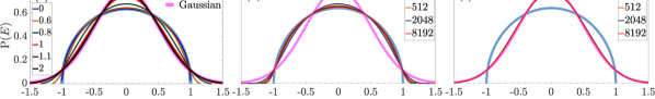
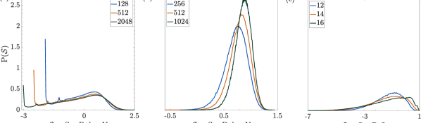
As a starting point we look at the DOS, which is the marginal PDF of energy levels. The bulk eigenvalues of -ensemble roughly scale with system size as [58]. So we scale the eigenvalues as and obtain the DOS numerically, as shown in Fig. 1(a) for and various . For we obtain such that the DOS converges to the Gaussian distribution, with increasing , as illustrated in Fig. 1(c) for a specfic value of . Exactly at , the DOS is system size independent and follows a shape intermediate between Gaussian distribution and Wigner semi-circle law since . But for , the DOS converges to the semicircle law upon increasing , as shown in Fig. 1(b) for a specific value of . However, in the limit (i.e. and ), all the eigenvalues of -ensemble freeze and produce a picket-fence spectrum [59]. A qualitative evolution of the shape of the DOS in - plane is shown in Fig. 2 of [35].
In case of the RPE, bulk eigenvalues scale as: . Consequently the scaled DOS of RPE () varies from Wigner’s semicircle to Gaussian similar to -ensemble as is increased from . Contrarily for 1-D disordered spin-1/2 Heisenberg model, DOS always follows a Gaussian distribution spreading with the disorder strength, which is typical of many-body systems with local interactions [60]. However, the differences in global shapes of DOS from these different models do not dictate the correlations in the respective local energy scales as demonstrated below.
Nearest Neighbour Spacing (NNS):
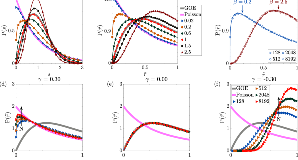
One of the most commonly investigated quantity reflecting local spectral correlations is the distribution of NNS of the ordered and unfolded eigenvalues (see Appx. A), which follows Wigner’s surmise and exponential distribution for the chaotic and integrable systems respectively [7]. As the nature of correlation present in the spectrum edge is different than that of the bulk energy levels, we numerically evaluate the PDF of NNS choosing only middle 25% of the spectrum. The results for are shown in Fig. 2(a) via markers along with the approximate empirical PDF of NNS (Eqs. (12) and (13) in [35]), which is -independent, provided . Such a functional form also implies that for , , thus the degree of level repulsion is indeed quantified via , as expected from Eq. (1). We observe a crossover from Wigner’s surmise to exponential distribution in Fig. 2(a) as we decrease , implying a suppression of chaos. A similar crossover is observed in RPE [61] and 1-D disordered spin-1/2 Heisenberg model [62] as well.
Ratio of Nearest Neighbour Spacing (RNNS):
Another notable measure of the short-range spectral correlations is the RNNS, which is much simpler to study since unfolding of the energy spectrum is not required [63, 64]. If we define , where is the RNNS, then , with being the Heaviside step function. We show PDF of via markers in Fig. 2(b) for along with the empirical PDF of RNNS (Eq. (1) in [65]). Again a crossover w.r.t. is immediately apparent. For , the density of RNNS is system size independent, as shown in Fig. 2(c) for two values of while varying . This can inferred from Fig. 3(a) as well, where the ensemble averaged values of as a function of collapse for different provided . In Figs. 2(d), (e) and (f), we show the density of for different values of while varying . For any value of as (i.e. ), the energy levels are highly correlated and strongly repel each other. The increase in level repulsion with is shown in Fig. 2(f) for a fixed value of . Exactly at (i.e. ) the density of is independent of and matches that of GOE (Fig. 2(e)). On the other hand for any and (i.e. ), the energy levels become uncorrelated and clustered as in Poisson ensemble. In Fig. 2(d) we show that the density of converges towards Poisson expression as we increase for a fixed value of . The analyses above imply that the signatures of chaos in the short-range spectral correlations are lost as we lower the repulsion parameter . Now we identify the exact nature of such a transition.
Criticality in chaotic-integrable transition:
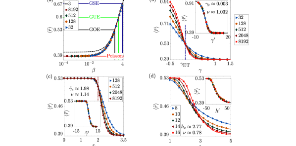
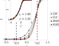
For a fixed , the quick convergence of PDF of RNNS with system size (Fig. 3(a)) enables us to conclude that the has one to one correspondence with when . increases with for any (as ), hence should also increase with and vice versa. Figure 3(b) conforms to the above expectations suggesting a scaling hypothesis for . Let us assume that there exists a relevant correlation length showing a power law divergence around a critical point, , i.e. , where is a critical exponent. Then any quantity showing non-analytical behaviour close to should behave as
| (7) |
where is a universal function and we assume to scale with instead of . Such a scaling ansatz valid for order phase transition is shown to hold in case of the Kullback-Leibler divergence of RPE [61]. We collapse the crossover curves from different system sizes based on Eq. (7) (see Appx. A) and obtain and as shown in the inset of Fig. 3(b). Such a critical behaviour can also be inferred from the scale invariance of w.r.t. (Fig. 3(a)). Comparing this with Eq. (7), we get and , which is consistent with our numerical analysis.
We show the curves for different system sizes and chain lengths in Fig. 3(c) and (d) for RPE and Heisenberg model respectively. Again assuming a power law behaviour like Eq. (7), we are able to collapse the data for RPE using . For Heisenberg chain we assume that and get . Note that the critical disorder strength found here corresponds to the middle 25% of eigenspectrum, hence conforms to the energy density phase diagram of MBL transition present in the literature [55].
Thus we show that the chaotic-integrable transition in all three models is order in nature. The crucial difference lies in the physical significance of these critical points. We observe that the chaotic-integrable transition occurs at in the case of RPE, i.e. the energy states localize as soon as the energy levels start to cluster. Contrarily in case of -ensemble, chaotic-integrable transition occurs at which we previously argued to be , i.e. where ergodicity breaks down. Thus in the thermodynamic limit (), there will be extended states for which energy levels are uncorrelated, which has a profound implication in the dynamical properties of -ensemble (Sec. 4). Thus our analysis shows that the eigenstate localization property is not necessarily indicative of the degree of repulsion present in the energy spectrum as also observed in certain structured matrix ensembles [66, 67, 68].
Power spectrum:
Short-range spectral correlations in -ensemble exhibit criticality only around . We also expect a second critical point associated with the localization transition, which can be captured by the long-range spectral correlations, e.g. power spectrum of statistics defined as [69, 70],
| (8) |
where is the fluctuation of the unfolded energy level, around its mean value, . Ensemble average of , denoted by , is explored for 1-D disordered spin-1/2 Heisenberg model in [71, 72]. For , there exists a critical frequency in -ensemble [73] such that for identifying completely chaotic behaviour whereas for , which is a signature of Poisson ensemble. Note that the power spectrum of some physical systems like Robnik billiard [74], kicked top [75] exhibit a homogeneous behaviour, , across all frequencies with .
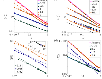
In Fig. 4(a), we show the power spectrum of -ensemble as a function of dimensionless frequency, for and various with the bold curves showing the analytical forms of for Poisson and GOE (Eq. (10) in [69]). In Fig. 4(b), we show for same values of but also by varying denoted by different colors. We see that for finite and , for a typical value of . However, we observe that for and (i.e. ), there are fluctuations around behavior due to the energy spectrum attaining a picket-fence structure. For , we can identify two critical points separating three distinct regimes by looking at Fig. 4(b) or from the analytical calculations in [73]:
-
•
: for any energy levels are correlated at all scales even in the thermodynamic limit
-
•
: Heterogeneous spectra separating Poisson and GOE like scaling. In Fig. 4(c), we show for and various , which clearly reflects the heterogeneous features. In the inset we show numerically obtained vs. .
-
•
: for any energy levels are uncorrelated at all scales even in the thermodynamic limit
Note that for and , i.e. signature of chaotic spectrum prevails over infinitely many frequencies. However, their support set constitute a zero fraction of the set of principle frequencies as for any ( is the highest frequency required to fully reconstruct the original spectrum [69]). Such a fractal behaviour suggests the absence of ergodicity in the -ensemble for . For example, in case of RPE, eigenstates occupy zero fraction of the Hilbert space volume despite being extended in the NEE phase () [56]. Corresponding power spectrum also exhibits heterogeneous behaviour as shown in Fig. 4(d). Thus we can attribute the heterogeneity in power spectrum of statistics to the existence of NEE phase and we can conclude that -ensemble enters the NEE phase for where ergodicity breaks down at and Anderson transition occurs at .
With this primary evidence of the existence of NEE regime in -ensemble, in the next section we will study the eigenfunction properties and obtain the fractal scaling of NEE states.
3 Properties of Eigenstates
Due to the canonical invariance, the eigenvectors of GOE matrices are uniformly distributed in the unit -dimensional sphere, resulting in mutually independent eigenvector components. Contrarily for -ensemble, all elements but the first component of the eigenvector can be expressed in terms of the eigenvalue and different matrix elements [36]. Hence even for typical values of (i.e. ), the eigenvector properties of Wigner-Dyson and -ensemble are different from each other, although their energy level statistics are identical. This can be readily verified from the distribution of ( is component of the eigenstate ), which has a long tail for in -ensemble compared to GOE.
Localization transition:
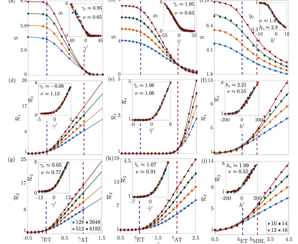
In order to characterize the Anderson transition from the properties of eigenstates, we begin by computing the Shannon entropy, defined as, with . In Fig. 5(a), we show ensemble averaged S, obtained from the eigenstates taken from middle 25% of the spectra, exhibiting a non-analyticity around . Assuming a power-law behaviour of the relevant correlation length, we obtain critical parameter and exponent using Eq. (7), while the collapsed data is shown in the inset of Fig. 5(a). We also observe that the Inverse Participation Ratio (IPR), I exhibits a criticality around as shown in Fig. 6. Thus we confirm that the Anderson transition occurs at for -ensemble, while at for RPE [Fig. 5(b)].
For 1-D disordered spin-1/2 Heisenberg model, Shannon entropy is almost constant for a particular if disorder strength is small () and slowly decaying for . Similar behaviour for IPR indicates that the energy states of the Heisenberg model in the MBL regime are extended in the Hilbert space exhibiting a non-trivial multifractal behaviour [55]. However according to [54], one may look at the ratio of Shannon entropies of Heisenberg model and GOE, i.e. , where is the Hilbert space dimension of the symmetry sector. The finite-size scaling of gives the numerical estimate of the MBL transition point to be for our choice of . This is the same critical point beyond which energy levels start to cluster [Fig. 3(d)]. Such a conclusion is also verified via studies of entanglement entropy, magnetization fluctuations [55]. Thus unlike -ensemble, eigenstates start to localize as soon as energy levels begin to cluster for both RPE and 1-D disordered spin-1/2 Heisenberg model.
Ergodic to non-ergodic transition:
We now quantify the loss of ergodicity by computing the relative Rényi () entropy between a pair of eigenfunctions [76] having similar energy densities. Let be the eigenvector of the disordered realization of an ensemble. We define two kinds of as follows:
| (9) | ||||
Here and measure similarity among wavefunctions obtained from the same and different samples respectively. For eigenstates of GOE, , where are i.i.d. random variables and for , assuming wavefunctions are normalized. Then, , where is the modified Bessel function of kind. Then,
| (10) | ||||
Thus for any pair of completely extended wavefunctions and this value is used to benchmark our numerical estimates. The relative Rényi entropy can be viewed as a generalization of the Kullback-Leibler divergence exhibiting critical behaviour in the case of RPE [61]. We will investigate and in the similar spirit with the premises of finding:
-
•
Ergodic regime: for any pair of wavefunctions, as both of them are uniformly extended
-
•
Localized regime: will diverge as different wavefunctions localize at separate sites
-
•
Non-ergodic regime having two possibilities:
-
–
If energy levels of repel each other, then such energy states come from the same symmetry sector, i.e. the same subspace of the Hilbert space. Thus are likely to hybridize if the governing Hamiltonian is sufficiently dense [61], giving .
-
–
In absence of any level repulsion, the energy states in the NEE phase are likely to be extended over different parts of the Hilbert space, thus will diverge.
-
–
Let us now illustrate the measures for the well studied case of RPE. For two nearby energy states with comparable energy densities, for and for as chaotic-integrable transition occurs at . On the other hand, the energy states from different samples, say , are likely to have different support set in the NEE phase, as different governing Hamiltonians cannot hybridize them even if their energy densities are comparable giving for . In Fig. 5(e) and (h) we show for RPE exhibiting order phase transitions clearly identifying the critical points and respectively.
Recall that for -ensemble chaotic-integrable transition occurs at , hence should show non-analyticity at the same point. Previously we argued that is also the ergodic transition point, thus should exhibit criticality there as well. The critical behaviours of are evident in Fig. 5(d) and (g), where scaling analysis gives .
In the case of 1-D disordered spin-1/2 Heisenberg model, we find that the scaling of indicate a in Fig. 5(i) while earlier we identified . This indicates the existence of NEE in 1-D disordered spin-1/2 Heisenberg model for an intermediate range of disorder in agreement with the existing study on participation entropy, survival probability [54] and momentum distribution fluctuations [71]. Therefore one would expect to show criticality at since it is also the chaotic-integrable transition point. However the Hamiltonians of 1-D disordered spin-1/2 Heisenberg model are so sparse that they fail to completely hybridize the NEE eigenstates even from the same subspace of the Hilbert space. As a result shows criticality at [Fig. 5(f)], a value in between and . Below the critical values, in all three models as expected from Eq. (10).
Localization length:
In the previous section, we noticed that the spectral properties of -ensemble and RPE have an important difference: chaotic-integrable transition occurs at for -ensemble and for RPE. The degree of level repulsion, has been interpreted as the rescaled localization length in various systems [77, 78, 79, 80] though there are exceptions as well [81]. Now we look at the entropic localization length w.r.t. the Shannon entropy, , such that or for a fully ergodic or localized energy state respectively [77]. In case of RPE or 1-D disordered spin-1/2 Heisenberg model, one can numerically fit the PDF of NNS with any phenomenological model (e.g. Brody [18], Berry-Robnik [19] etc.) to estimate the repulsion parameter, . However, such a numerical fit pertains to the global shape of the PDF of NNS [77], without necessarily reflecting the behaviour of , which is the true measure of level repulsion in a system. Thus we exploit the one to one correspondence between and the mean value of RNNS. We observe a sub-linear behaviour when is small and converges to 1 when [Fig. 7(b) and (c)]. Hence energy states are completely extended whenever the energy levels repel each other and this justifies the coincidence of chaotic-integrable transition with the delocalization-localization transition in RPE and 1-D disordered spin-1/2 Heisenberg model.
We show as a function of for various system sizes in case of -ensemble in Fig. 7(a). Here the relationship between the localization length and the degree of level repulsion is super-linear throughout. Moreover, becomes independent of for while as shown in the inset of Fig. 7(a). This implies that the localization transition should occur roughly at as chaotic-integrable transition occurs at . This supports our earlier observation that does not coincide with the chaotic-integrable transition point in the case of -ensemble unlike RPE or Heisenberg model.
Scaling of eigenstate fluctuations:
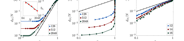
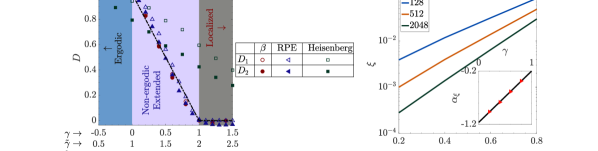
It is important to analyse the eigenfunction fluctuations which can be quantified via Rényi entropy, where ’s are fractal dimensions for different values of [82]. For , the Rényi entropy converges to the Shannon entropy, . Similarly for , one obtains the scaling in IPR . In the ergodic regime the fractal dimensions, as eigenstates occupy the full Hilbert space volume, while in the localized regime. In the NEE phase, , which implies that the eigenstates are extended over infinitely many but a zero fraction of all possible sites in the thermodynamic limit (i.e. but if ). Since distributions of Shannon entropy and IPR are quite broad and skewed (Fig. 9(a)), median instead of mean has been used to estimate such fractal dimensions [83]. The numerically estimated clearly identifies the ergodic, NEE and localized regimes for -ensemble and RPE as shown in Fig. 8 ( and in the NEE phase for -ensemble and RPE respectively). However, in the case of Heisenberg model, does not vanish for resulting from non-trivial multifractality in the MBL phase [55].
To probe finer details of the eigenstructure of -ensemble, we look at the density of Shannon entropy. The distributions from different system sizes collapse on top of each other at upon a rescaling . However, in the NEE phase (), two peaks emerge in the histogram of S: i) a broad peak whose location roughly scales as , ii) a sharp peak at , whose height decreases with (Fig. 9(a)). The existence of the peak (which is absent for RPE, Fig. 9(b) and Heisenberg model, Fig. 9(c)) implies that a small albeit finite fraction of eigenstates are localized for . In Fig. 8(b), we show , the fraction of localized eigenstates as a function of for various . Inset of the same figure shows , the system size scaling exponent of , which implies roughly . Thus in the thermodynamic limit, there will be an infinite number of completely localized states in the intermediate regime of -ensemble (since for ), which constitutes a zero fraction of all possible eigenstates (since for ). By looking at the median and mode of IPR of individual eigenstates for different system sizes, we find that the high energy states (i.e. the ones in the middle of spectrum) have a greater tendency to be localized compared to the ones close to the ground state in the NEE regime. Thus contrary to RPE, -ensemble offers two kinds of eigenstates in the NEE phase: number of completely localized and number of NEE states.
4 Properties of Dynamics
So far we have looked at the statistical picture of the energy level correlation, eigenstate localization end ergodic properties of -ensemble. Now we want to look at the dynamical aspects of -ensemble, revealing important time and energy scales. In this regard, one of the largest time scales is the Heisenberg time, defined as the inverse of mean level spacing. Beyond such a time, the energy level dynamics of a system equilibrates e.g. the spectral form factor attains a stationary state [84]. Now we explicitly look at the time evolution of an initially localized state and identify the relevant dynamical timescales.
Survival probability:
An important characterization of the dynamics of a quantum mechanical system is often done by monitoring the time evolution of a given wavefunction. We choose a unit vector having energy close to the spectrum centre of as our initial state. Let be the eigenpair of such that the time evolution of the initial state is given by,
| (11) |
The spread of initial state over all other states is controlled by the off-diagonal terms in and is quantified by the survival probability [85]
| (12) |
In general, the survival probability decays till , known as the Thouless time [86]. This is the time required for to maximally spread over the Hilbert space. For example, in disordered (ergodic) metals, a particle diffuses to the sample boundaries within . The inverse of gives the Thouless energy, below which the spectral correlations are similar to those of Wigner-Dyson ensemble. Moreover, a finite-sized closed quantum system always equilibrates [87] and the equilibrium value of survival probability is given by
| (13) |
Thus is the IPR of initial state in the eigenbasis . The time required to reach is known as the relaxation time, . The gap between and is known as the correlation hole, . A finite is a direct manifestation of the spectral rigidity, i.e. the presence of long range correlation among energy levels [88, 54, 89].
The time evolution of survival probability for -ensemble is shown in Fig. 10(a) and (b) for various system sizes and values. Tuning , we observe three qualitatively different behaviours as follows:
1. Ergodic regime The correlation hole is always present with easily identifiable Thouless and relaxation times. exhibits an approximately scaling close to (inset of Fig. 10(a)), which can be understood from sparsity of the Hamiltonian. Contrarily in the ergodic regime of RPE, is independent of system size due to the presence of all to all coupling [56, 90]. We also observe that within , is non-monotonic unlike 1-D disordered spin-1/2 Heisenberg model [85].
2. NEE phase We show as a function of for different system sizes in Fig. 10(c) where for . The inset shows that as increases. Recall that chaotic-integrable transition occurs at , beyond which long range correlation among energy levels (e.g. see power spectrum) is lost. The spectral rigidity is necessary for the existence of [88], which explains the absence of correlation hole in the NEE regime in the thermodynamic limit. On the other hand, a finite exists in the NEE phases of RPE and 1-D disordered spin-1/2 Heisenberg model, as chaotic-integrable transition occurs at and respectively.
3. Localized phase Exactly at , we observe survival probability curves from different system sizes to collapse on top of each other, showing a critical behaviour similar to RPE. In the localized regime (i.e. ), is completely absent while converges to 1 upon increasing either or .
We show the equilibrium value of survival probability, , as a function of in Fig. 10(d). We observe that for which is expected as the initial state, is an eigenstate in the localized regime. Inset of Fig. 10(d) shows system size scaling of , indicating that in the NEE regime denoting the extent of spread over the Hilbert space for an initially localized state.
5 Conclusions
In this work we study the spectral properties of -ensemble with a motivation that the competition between diagonal and off-diagonal terms may lead to a NEE phase. As customary in random matrix theory, we discuss the DOS and short-range spectral correlations, namely, NNS, RNNS and observe a transition from chaos to integrability at . The next pertinent question is whether this transition can be associated with the ergodic and/or localization transitions. A simple analysis of the power spectrum of noise in the eigensequence identifies two critical points: ergodic transition at and Anderson transition at , separating three distinct phases: ergodic (), NEE () and localized () phase. Thus similar to RPE [56], related ensembles [91, 92] and certain floquet systems [93, 94, 95], -ensemble is another matrix model where NEE phase exists over a finite interval of system parameters.
The above observations can be consolidated from the eigenfunction properties as both Shannon entropy and IPR show criticality at , confirming it to be the Anderson transition point. The system size scaling of the above quantities gives us the fractal dimensions , clearly demarcating the three phases. For Relative Rényi entropies of type 1 and 2, criticality is seen at , thus confirming it to be the chaotic-integrable as well as the ergodic transition point. Moreover, the distribution of Shannon entropy indicates that in the NEE phase, there is a coexistence of number of completely localized and number of NEE states.
Finally, we identify the relevant dynamical timescales from the time evolution of the survival probability, of an initially localized state and find that the correlation hole, , is always present in the ergodic regime and absent in the NEE phase for as energy levels become uncorrelated. Moreover for and as expected in a localized phase. The NEE phase in -ensemble is quite distinct from that in RPE, where the energy levels repel each other since integrability breaks down at the Anderson transition point. Again the chaotic-integrable transition point is energy density dependent and ergodicity breaks at a lower disorder strength in the case of 1-D disordered spin-1/2 Heisenberg model. We calculate the entropic localization length to explain why chaotic-integrable transition in -ensemble does not coincide with the localization transition point. These subtle differences imply that -ensemble is not a suitable model for spin systems like 1-D disordered spin-1/2 Heisenberg model. The proposition that -ensemble can model Heisenberg chain [62] has also been contradicted in [96, 97] via analyses of higher order level spacings, Spectral Form Factor (SFF) and in [65] by studying RNNS crossover. However, we observe that in the ergodic regime of the -ensemble, Thouless time scales with the system size similar to sparse Hamiltonians [85]. Thus our analyses suggest that the -ensemble can imitate the spectral properties of various Hamiltonians provided ergodicity breaks down at the chaotic-integrable transition point in such systems.
Acknowledgment: We thank Lea F. Santos and Ivan Khaymovich for many useful comments on the manuscript. AKD is supported by INSPIRE Fellowship, DST, India.
Appendix A Numerical details
Unfolding:
For fixed values of system parameters and size, we obtain , the cumulative density of eigenvalues from all disordered realizations. Next we smooth using a moving average filter. Then for the original eigenvalue , unfolding implies the interpolation of [10].
Scaling of crossover curves:
Let us look at an observable for a system parameter . If we observe non-analytical behavior of the corresponding crossover curves from different system sizes, we assume to behave according to Eq. (7). So we take an array of parameters and measure for two system sizes and , giving us two arrays . Following Eq. (7), we take the function . Now define the function for . For the correct guess of and , vs. and vs. should behave similarly. The observed non-analyticity of the curves vs. and vs. gives a good idea of the initial value of and we take as the starting value. For these initial guesses of and , we interpolate vs. w.r.t. to create a new array . Next we calculate the Residual Sum of Squares (RSS) between and , defined as . Since RSS should be 0 for the correct choice of and , we iteratively change and to minimize the RSS, which gives us the desired values of and for and . We repeat this exercise for all pairs of system sizes and report the average of the obtained parameters.
References
- [1] F. J. Dyson, “The threefold way. algebraic structure of symmetry groups and ensembles in quantum mechanics,” Journal of Mathematical Physics, vol. 3, no. 6, pp. 1199–1215, 1962.
- [2] A. Altland and M. R. Zirnbauer, “Nonstandard symmetry classes in mesoscopic normal-superconducting hybrid structures,” Phys. Rev. B, vol. 55, pp. 1142–1161, Jan 1997.
- [3] D. A. Ivanov, Random-Matrix Ensembles in p-Wave Vortices, pp. 253–265. Berlin, Heidelberg: Springer Berlin Heidelberg, 2002.
- [4] A. Dubbs, A. Edelman, P. Koev, and P. Venkataramana, “The beta-wishart ensemble,” Journal of Mathematical Physics, vol. 54, no. 8, p. 083507, 2013.
- [5] A. Dubbs and A. Edelman, “The beta-manova ensemble with general covariance,” Random Matrices: Theory and Applications, vol. 03, no. 01, p. 1450002, 2014.
- [6] R. Killip and I. Nenciu, “Matrix models for circular ensembles,” International Mathematics Research Notices, vol. 2004, no. 50, pp. 2665–2701, 2004.
- [7] M. Mehta, Random Matrices. Pure and Applied Mathematics, Elsevier Science, 2004.
- [8] F. Borgonovi, F. Izrailev, L. Santos, and V. Zelevinsky, “Quantum chaos and thermalization in isolated systems of interacting particles,” Physics Reports, vol. 626, pp. 1 – 58, 2016. Quantum chaos and thermalization in isolated systems of interacting particles.
- [9] O. Bohigas, M. J. Giannoni, and C. Schmit, “Characterization of chaotic quantum spectra and universality of level fluctuation laws,” Phys. Rev. Lett., vol. 52, pp. 1–4, Jan 1984.
- [10] T. Guhr, A. Müller–Groeling, and H. A. Weidenmüller, “Random-matrix theories in quantum physics: common concepts,” Physics Reports, vol. 299, no. 4, pp. 189 – 425, 1998.
- [11] E. A. Yuzbashyan, B. L. Altshuler, and B. S. Shastry, “The origin of degeneracies and crossings in the 1d hubbard model,” Journal of Physics A: Mathematical and General, vol. 35, pp. 7525–7547, aug 2002.
- [12] E. Corrigan and R. Sasaki, “Quantum versus classical integrability in calogero$ndash$moser systems,” Journal of Physics A: Mathematical and General, vol. 35, pp. 7017–7061, aug 2002.
- [13] M. Berry and M. Tabor, “Level clustering in the regular spectrum,” Proceedings of the Royal Society of London A: Mathematical, Physical and Engineering Sciences, vol. 356, no. 1686, pp. 375–394, 1977.
- [14] F. Haake, M. Kuś, and R. Scharf, “Classical and quantum chaos for a kicked top,” Zeitschrift für Physik B Condensed Matter, vol. 65, pp. 381–395, Sep 1987.
- [15] A. Y. Abul-Magd, B. Dietz, T. Friedrich, and A. Richter, “Spectral fluctuations of billiards with mixed dynamics: From time series to superstatistics,” Phys. Rev. E, vol. 77, p. 046202, Apr 2008.
- [16] S. N. Evangelou and J.-L. Pichard, “Critical quantum chaos and the one-dimensional harper model,” Phys. Rev. Lett., vol. 84, pp. 1643–1646, Feb 2000.
- [17] B. I. Shklovskii, B. Shapiro, B. R. Sears, P. Lambrianides, and H. B. Shore, “Statistics of spectra of disordered systems near the metal-insulator transition,” Phys. Rev. B, vol. 47, pp. 11487–11490, May 1993.
- [18] T. Brody, “A statistical measure for the repulsion of energy levels,” Lettere al Nuovo Cimento (1971-1985), vol. 7, no. 12, pp. 482–484, 1973.
- [19] M. V. Berry and M. Robnik, “Semiclassical level spacings when regular and chaotic orbits coexist,” Journal of Physics A: Mathematical and General, vol. 17, no. 12, p. 2413, 1984.
- [20] F. Izrailev, “Quantum localization and statistics of quasienergy spectrum in a classically chaotic system,” Physics Letters A, vol. 134, no. 1, pp. 13 – 18, 1988.
- [21] N. Rosenzweig and C. E. Porter, “Repulsion of energy levels in complex atomic spectra,” Phys. Rev., vol. 120, pp. 1698–1714, Dec 1960.
- [22] J. X. de Carvalho, M. S. Hussein, M. P. Pato, and A. J. Sargeant, “Symmetry-breaking study with deformed ensembles,” Phys. Rev. E, vol. 76, p. 066212, Dec 2007.
- [23] G. Casati, L. Molinari, and F. Izrailev, “Scaling properties of band random matrices,” Phys. Rev. Lett., vol. 64, pp. 1851–1854, Apr 1990.
- [24] A. D. Mirlin, Y. V. Fyodorov, F.-M. Dittes, J. Quezada, and T. H. Seligman, “Transition from localized to extended eigenstates in the ensemble of power-law random banded matrices,” Phys. Rev. E, vol. 54, pp. 3221–3230, Oct 1996.
- [25] F. Toscano, R. O. Vallejos, and C. Tsallis, “Random matrix ensembles from nonextensive entropy,” Physical Review E, vol. 69, no. 6, p. 066131, 2004.
- [26] A. Y. Abul-Magd, “Random matrix theory within superstatistics,” Phys. Rev. E, vol. 72, p. 066114, Dec 2005.
- [27] C. M. Canali, “Model for a random-matrix description of the energy-level statistics of disordered systems at the anderson transition,” Phys. Rev. B, vol. 53, pp. 3713–3730, Feb 1996.
- [28] A. Pandey and M. L. Mehta, “Gaussian ensembles of random hermitian matrices intermediate between orthogonal and unitary ones,” Communications in Mathematical Physics, vol. 87, pp. 449–468, Dec 1983.
- [29] P. Bántay and G. Zala, “Ultrametric matrices and representation theory,” Journal of Physics A: Mathematical and General, vol. 30, pp. 6811–6820, oct 1997.
- [30] F. J. Dyson, “Statistical theory of the energy levels of complex systems. i,” Journal of Mathematical Physics, vol. 3, no. 1, pp. 140–156, 1962.
- [31] P. J. Forrester, Log-gases and random matrices (LMS-34). Princeton University Press, 2010.
- [32] T. H. Baker and P. J. Forrester, “The calogero-sutherland model and generalized classical polynomials,” Communications in Mathematical Physics, vol. 188, no. 1, pp. 175–216, 1997.
- [33] P. Choquard, “Coulomb system equivalent to the energy spectrum of the calogero-sutherland-moser (csm) model,” Journal of statistical physics, vol. 89, no. 1, pp. 61–68, 1997.
- [34] G. Livan, M. Novaes, and P. Vivo, Classified Material, pp. 53–56. Cham: Springer International Publishing, 2018.
- [35] G. Le Caër, C. Male, and R. Delannay, “Nearest-neighbour spacing distributions of the -hermite ensemble of random matrices,” Physica A: Statistical Mechanics and its Applications, vol. 383, no. 2, pp. 190–208, 2007.
- [36] I. Dumitriu and A. Edelman, “Matrix models for beta ensembles,” Journal of Mathematical Physics, vol. 43, no. 11, pp. 5830–5847, 2002.
- [37] A. Pandey, “Statistical properties of many-particle spectra: Iii. ergodic behavior in random-matrix ensembles,” Annals of Physics, vol. 119, no. 1, pp. 170–191, 1979.
- [38] I. Dumitriu, A. Edelman, and G. Shuman, “Mops: Multivariate orthogonal polynomials (symbolically),” Journal of Symbolic Computation, vol. 42, no. 6, pp. 587–620, 2007.
- [39] J. T. Albrecht, C. P. Chan, and A. Edelman, “Sturm sequences and random eigenvalue distributions,” Foundations of Computational Mathematics, vol. 9, no. 4, pp. 461–483, 2009.
- [40] K. Johansson, “On fluctuations of eigenvalues of random Hermitian matrices,” Duke Mathematical Journal, vol. 91, no. 1, pp. 151 – 204, 1998.
- [41] P. Desrosiers and P. J. Forrester, “Hermite and laguerre -ensembles: Asymptotic corrections to the eigenvalue density,” Nuclear Physics B, vol. 743, no. 3, pp. 307–332, 2006.
- [42] R. Killip and M. Stoiciu, “Eigenvalue statistics for CMV matrices: From Poisson to clock via random matrix ensembles,” Duke Mathematical Journal, vol. 146, no. 3, pp. 361 – 399, 2009.
- [43] P. Forrester, “Global fluctuation formulas and universal correlations for random matrices and log-gas systems at infinite density,” Nuclear Physics B, vol. 435, no. 3, pp. 421–429, 1995.
- [44] A. B. De Monvel, L. Pastur, and M. Shcherbina, “On the statistical mechanics approach in the random matrix theory: integrated density of states,” Journal of statistical physics, vol. 79, no. 3, pp. 585–611, 1995.
- [45] B. Valkó and B. Virág, “Continuum limits of random matrices and the brownian carousel,” Inventiones mathematicae, vol. 177, no. 3, pp. 463–508, 2009.
- [46] A. Edelman and B. D. Sutton, “From random matrices to stochastic operators,” Journal of Statistical Physics, vol. 127, no. 6, pp. 1121–1165, 2007.
- [47] J. Ramirez, B. Rider, and B. Virág, “Beta ensembles, stochastic airy spectrum, and a diffusion,” Journal of the American Mathematical Society, vol. 24, no. 4, pp. 919–944, 2011.
- [48] L. Dumaz and B. Virág, “The right tail exponent of the Tracy–Widom distribution,” Annales de l’Institut Henri Poincaré, Probabilités et Statistiques, vol. 49, no. 4, pp. 915 – 933, 2013.
- [49] G. Borot, B. Eynard, S. N. Majumdar, and C. Nadal, “Large deviations of the maximal eigenvalue of random matrices,” Journal of Statistical Mechanics: Theory and Experiment, vol. 2011, p. P11024, nov 2011.
- [50] R. Allez and L. Dumaz, “Tracy–widom at high temperature,” Journal of Statistical Physics, vol. 156, no. 6, pp. 1146–1183, 2014.
- [51] A. Edelman, P.-O. Persson, and B. D. Sutton, “Low-temperature random matrix theory at the soft edge,” Journal of Mathematical Physics, vol. 55, no. 6, p. 063302, 2014.
- [52] A. K. Das and A. Ghosh, “Eigenvalue statistics for generalized symmetric and hermitian matrices,” Journal of Physics A: Mathematical and Theoretical, vol. 52, p. 395001, sep 2019.
- [53] L. F. Santos, “Integrability of a disordered heisenberg spin-1/2 chain,” Journal of Physics A: Mathematical and General, vol. 37, pp. 4723–4729, apr 2004.
- [54] E. J. Torres-Herrera and L. F. Santos, “Extended nonergodic states in disordered many-body quantum systems,” Annalen der Physik, vol. 529, no. 7, p. 1600284, 2017.
- [55] D. J. Luitz, N. Laflorencie, and F. Alet, “Many-body localization edge in the random-field heisenberg chain,” Phys. Rev. B, vol. 91, p. 081103, Feb 2015.
- [56] V. E. Kravtsov, I. M. Khaymovich, E. Cuevas, and M. Amini, “A random matrix model with localization and ergodic transitions,” New Journal of Physics, vol. 17, p. 122002, dec 2015.
- [57] J. Schenker, “Eigenvector localization for random band matrices with power law band width,” Communications in Mathematical Physics, vol. 290, no. 3, pp. 1065–1097, 2009.
- [58] I. Dumitriu and A. Edelman, “Global spectrum fluctuations for the -hermite and -laguerre ensembles via matrix models,” Journal of Mathematical Physics, vol. 47, no. 6, p. 063302, 2006.
- [59] J. Gustavsson, “Gaussian fluctuations of eigenvalues in the gue,” Annales de l’I.H.P. Probabilités et statistiques, vol. 41, no. 2, pp. 151–178, 2005.
- [60] T. A. Brody, J. Flores, J. B. French, P. A. Mello, A. Pandey, and S. S. M. Wong, “Random-matrix physics: spectrum and strength fluctuations,” Rev. Mod. Phys., vol. 53, pp. 385–479, Jul 1981.
- [61] M. Pino, J. Tabanera, and P. Serna, “From ergodic to non-ergodic chaos in rosenzweig–porter model,” Journal of Physics A: Mathematical and Theoretical, vol. 52, p. 475101, oct 2019.
- [62] W. Buijsman, V. Cheianov, and V. Gritsev, “Random matrix ensemble for the level statistics of many-body localization,” Physical review letters, vol. 122, no. 18, p. 180601, 2019.
- [63] Y. Y. Atas, E. Bogomolny, O. Giraud, and G. Roux, “Distribution of the ratio of consecutive level spacings in random matrix ensembles,” Phys. Rev. Lett., vol. 110, p. 084101, Feb 2013.
- [64] V. Oganesyan and D. A. Huse, “Localization of interacting fermions at high temperature,” Phys. Rev. B, vol. 75, p. 155111, Apr 2007.
- [65] A. L. Corps and A. Relaño, “Distribution of the ratio of consecutive level spacings for different symmetries and degrees of chaos,” Phys. Rev. E, vol. 101, p. 022222, Feb 2020.
- [66] W. Tang and I. M. Khaymovich, “Non-ergodic delocalized phase with poisson level statistics,” 2021.
- [67] T. Mondal, S. Sadhukhan, and P. Shukla, “Extended states with poisson spectral statistics,” Phys. Rev. E, vol. 95, p. 062102, Jun 2017.
- [68] T. Mondal and P. Shukla, “Statistical analysis of chiral structured ensembles: Role of matrix constraints,” Phys. Rev. E, vol. 99, p. 022124, Feb 2019.
- [69] E. Faleiro, J. M. G. Gómez, R. A. Molina, L. Muñoz, A. Relaño, and J. Retamosa, “Theoretical derivation of noise in quantum chaos,” Phys. Rev. Lett., vol. 93, p. 244101, Dec 2004.
- [70] R. Riser, V. A. Osipov, and E. Kanzieper, “Power spectrum of long eigenlevel sequences in quantum chaotic systems,” Phys. Rev. Lett., vol. 118, p. 204101, May 2017.
- [71] A. L. Corps, R. A. Molina, and A. Relaño, “Thouless energy challenges thermalization on the ergodic side of the many-body localization transition,” Phys. Rev. B, vol. 102, p. 014201, Jul 2020.
- [72] A. L. Corps and A. Relaño, “Long-range level correlations in quantum systems with finite hilbert space dimension,” Phys. Rev. E, vol. 103, p. 012208, Jan 2021.
- [73] A. Relaño, L. Muñoz, J. Retamosa, E. Faleiro, and R. A. Molina, “Power-spectrum characterization of the continuous gaussian ensemble,” Phys. Rev. E, vol. 77, p. 031103, Mar 2008.
- [74] J. M. G. Gómez, A. Relaño, J. Retamosa, E. Faleiro, L. Salasnich, M. Vraničar, and M. Robnik, “ noise in spectral fluctuations of quantum systems,” Phys. Rev. Lett., vol. 94, p. 084101, Mar 2005.
- [75] M. S. Santhanam and J. N. Bandyopadhyay, “Spectral fluctuations and noise in the order-chaos transition regime,” Phys. Rev. Lett., vol. 95, p. 114101, Sep 2005.
- [76] Á. Nagy and E. Romera, “Relative rényi entropy and fidelity susceptibility,” EPL (Europhysics Letters), vol. 109, p. 60002, mar 2015.
- [77] S. Sorathia, F. M. Izrailev, V. G. Zelevinsky, and G. L. Celardo, “From closed to open one-dimensional anderson model: Transport versus spectral statistics,” Phys. Rev. E, vol. 86, p. 011142, Jul 2012.
- [78] F. M. Izrailev, “Simple models of quantum chaos: Spectrum and eigenfunctions,” Physics Reports, vol. 196, no. 5, pp. 299–392, 1990.
- [79] G. Casati, B. V. Chirikov, I. Guarneri, and F. M. Izrailev, “Band-random-matrix model for quantum localization in conservative systems,” Phys. Rev. E, vol. 48, pp. R1613–R1616, Sep 1993.
- [80] J. Flores, L. Gutiérrez, R. A. Méndez-Sánchez, G. Monsivais, P. Mora, and A. Morales, “Anderson localization in finite disordered vibrating rods,” EPL (Europhysics Letters), vol. 101, p. 67002, mar 2013.
- [81] E. Benito-Matías and R. A. Molina, “Localization length versus level repulsion in one-dimensional driven disordered quantum wires,” Phys. Rev. B, vol. 96, p. 174202, Nov 2017.
- [82] Y. Y. Atas and E. Bogomolny, “Multifractality of eigenfunctions in spin chains,” Phys. Rev. E, vol. 86, p. 021104, Aug 2012.
- [83] A. D. Mirlin and F. Evers, “Multifractality and critical fluctuations at the anderson transition,” Phys. Rev. B, vol. 62, pp. 7920–7933, Sep 2000.
- [84] J. Šuntajs, J. Bonča, T. Prosen, and L. Vidmar, “Quantum chaos challenges many-body localization,” Phys. Rev. E, vol. 102, p. 062144, Dec 2020.
- [85] M. Schiulaz, E. J. Torres-Herrera, and L. F. Santos, “Thouless and relaxation time scales in many-body quantum systems,” Phys. Rev. B, vol. 99, p. 174313, May 2019.
- [86] D. Thouless, “Electrons in disordered systems and the theory of localization,” Physics Reports, vol. 13, no. 3, pp. 93–142, 1974.
- [87] A. J. Short, “Equilibration of quantum systems and subsystems,” New Journal of Physics, vol. 13, p. 053009, may 2011.
- [88] E. J. Torres-Herrera and L. F. Santos, “Dynamical manifestations of quantum chaos: correlation hole and bulge,” Philosophical Transactions of the Royal Society A: Mathematical, Physical and Engineering Sciences, vol. 375, no. 2108, p. 20160434, 2017.
- [89] T. Nosaka, D. Rosa, and J. Yoon, “The thouless time for mass-deformed syk,” Journal of High Energy Physics, vol. 2018, no. 9, pp. 1–40, 2018.
- [90] G. D. Tomasi, M. Amini, S. Bera, I. M. Khaymovich, and V. E. Kravtsov, “Survival probability in Generalized Rosenzweig-Porter random matrix ensemble,” SciPost Phys., vol. 6, p. 14, 2019.
- [91] G. Biroli and M. Tarzia, “Lévy-rosenzweig-porter random matrix ensemble,” Phys. Rev. B, vol. 103, p. 104205, Mar 2021.
- [92] I. M. Khaymovich, V. E. Kravtsov, B. L. Altshuler, and L. B. Ioffe, “Fragile extended phases in the log-normal rosenzweig-porter model,” Phys. Rev. Research, vol. 2, p. 043346, Dec 2020.
- [93] S. Ray, A. Ghosh, and S. Sinha, “Drive-induced delocalization in the aubry-andré model,” Phys. Rev. E, vol. 97, p. 010101, Jan 2018.
- [94] S. Roy, I. M. Khaymovich, A. Das, and R. Moessner, “Multifractality without fine-tuning in a Floquet quasiperiodic chain,” SciPost Phys., vol. 4, p. 25, 2018.
- [95] M. Sarkar, R. Ghosh, A. Sen, and K. Sengupta, “Mobility edge and multifractality in a periodically driven aubry-andré model,” Phys. Rev. B, vol. 103, p. 184309, May 2021.
- [96] P. Sierant and J. Zakrzewski, “Model of level statistics for disordered interacting quantum many-body systems,” Phys. Rev. B, vol. 101, p. 104201, Mar 2020.
- [97] P. Sierant and J. Zakrzewski, “Level statistics across the many-body localization transition,” Phys. Rev. B, vol. 99, p. 104205, Mar 2019.