Asymptotics of arithmetic functions of GCD and LCM of random integers in hyperbolic regions

Abstract.

We prove limit theorems for the greatest common divisor and the least common multiple of random integers. While the case of integers uniformly distributed on a hypercube with growing size is classical, we look at the uniform distribution on sublevel sets of multivariate symmetric polynomials, which we call hyperbolic regions. Along the way of deriving our main results, we obtain some asymptotic estimates for the number of integer points in these hyperbolic domains, when their size goes to infinity.

1. Introduction

Let $f:\mathbb{N}\to\mathbb{C}$ be an arithmetic function, with $\mathbb{N}$ denoting $\{1,2,\ldots\}$. The motivation for the present paper comes from the recent study of hyperbolic sums

$$f_{G}(n):=\sum_{ij\leqslant n}f({\rm GCD}\,(i,j))\quad\text{and}\quad f_{L}(n):=\sum_{ij\leqslant n}f({\rm LCM}\,(i,j))$$ (1.1)

carried out in [6], where the authors derived asymptotics of $f_{G}(n)$ and $f_{L}(n)$, as $n\to\infty$, for certain classes of arithmetic functions $f$. For example, Theorem 2.2 in [6] yields the following asymptotics

$$\lim_{n\to\infty}\frac{f_{G}(n)}{n\log n}=\frac{1}{\zeta(2)}\sum_{k=1}^{\infty}\frac{f(k)}{k^{2}},$$ (1.2)

provided that $f(n)=o(n^{\beta}\log^{\delta}n)$, as $n\to\infty$, for some $\beta<1$, $\delta\in\mathbb{R}$ and with $\zeta$ being the Riemann zeta-function.

To set up the scene, recast (1.1) and (1.2) in the probabilistic language as follows. Assume that on a certain probability space $(\Omega,\mathcal{F},\mathbb{P})$, there is a sequence of random vectors $\bigl{(}(V_{1}^{(n)},V_{2}^{(n)})\bigr{)}_{n\in\mathbb{N}}$ such that, for every fixed $n$, $(V_{1}^{(n)},V_{2}^{(n)})$ has a uniform distribution on the finite set

$$H_{2,2}(n):=\{(i_{1},i_{2})\in\mathbb{N}^{2}:i_{1}i_{2}\leqslant n\}$$

(the choice of notation $H_{2,2}$ will be explained below, see (2.1)). This means that, for all $(i_{1},i_{2})\in H_{2,2}(n)$,

$$\mathbb{P}\{(V_{1}^{(n)},V_{2}^{(n)})=(i_{1},i_{2})\}=\frac{1}{|H_{2,2}(n)|}.$$

Then

$$f_{G}(n)=|H_{2,2}(n)|\cdot\mathbb{E}f({\rm GCD}\,(V_{1}^{(n)},V_{2}^{(n)}))\quad\text{and}\quad f_{L}(n)=|H_{2,2}(n)|\cdot\mathbb{E}f({\rm LCM}\,(V_{1}^{(n)},V_{2}^{(n)})).$$ (1.3)

Taking into account the asymptotics

$$|H_{2,2}(n)|=\sum_{i_{1}=1}^{n}\sum_{i_{2}=1}^{\lfloor n/i_{1}\rfloor}1=\sum_{i_{1}=1}^{n}\lfloor n/i_{1}\rfloor~{}\sim~{}n\log n,\quad n\to\infty,$$

where $\lfloor x\rfloor$ denotes the integer part of $x\in\mathbb{R}$ and the notation $a_{n}\sim b_{n}$ means that $\lim_{n\to\infty}(a_{n}/b_{n})=1$, we conclude that (1.2) is equivalent to

$$\lim_{n\to\infty}\mathbb{E}f({\rm GCD}\,(V_{1}^{(n)},V_{2}^{(n)}))=\frac{1}{\zeta(2)}\sum_{k=1}^{\infty}\frac{f(k)}{k^{2}}.$$ (1.4)

Remarkably, the quantity on the right-hand side coincides with $\mathbb{E}f(U^{(2,\infty)})$, where by Theorem 1 in [5], the distribution of $U^{(2,\infty)}$ is the distributional limit of ${\rm GCD}\,(Z_{1}^{(n)},Z_{2}^{(n)})$ as $n\to\infty$, the pair $(Z_{1}^{(n)},Z_{2}^{(n)})$ being uniformly distributed in the square $\{1,2,\ldots,n\}^{2}$. Since (1.4) holds for all bounded arithmetic functions, it actually tells us that there is the convergence in distribution

$$\lim_{n\to\infty}\mathbb{P}\{{\rm GCD}\,(V_{1}^{(n)},V_{2}^{(n)})=m\}=\mathbb{P}\{U^{(2,\infty)}=m\},\quad m\in\mathbb{N}.$$

Therefore, ${\rm GCD}\,(V_{1}^{(n)},V_{2}^{(n)})$ for large $n$ behaves as the GCD of two independent integers picked uniformly at random from $\{1,2,\ldots,n\}$.

We shall show in the present paper that it is not a coincidence but rather a simple instance of a much deeper and general phenomenon. This observation will allow us to extend some results in [6] to an arbitrary dimension and cover more general hyperbolic regions defined by the standard symmetric polynomials.

Acknowledgments

We thank the anonymous referee for several useful comments and suggestions.

2. Hyperbolic regions and hyperbolic sums

Fix $r\in\mathbb{N}$ and $1\leqslant\ell\leqslant r$, and let $P_{\ell}(x_{1},x_{2},\ldots,x_{r})$ be the $\ell$-th standard symmetric polynomial in $r$ variables, that is,

$$P_{\ell}(x_{1},x_{2},\ldots,x_{r}):=\sum_{1\leqslant i_{1}<i_{2}<\cdots<i_{\ell}\leqslant r}x_{i_{1}}x_{i_{2}}\cdots x_{i_{\ell}}.$$

In particular,

$$P_{1}(x_{1},x_{2},\ldots,x_{r})=x_{1}+x_{2}+\cdots+x_{r}\quad\text{and}\quad P_{r}(x_{1},x_{2},\ldots,x_{r})=x_{1}x_{2}\cdots x_{r}.$$

Now we introduce ‘discrete’ hyperbolic regions in $\mathbb{N}^{r}$ given, for $n\geqslant\binom{r}{\ell}$, by

$$H_{\ell,r}(n):=\{(i_{1},\ldots,i_{r})\in\mathbb{N}^{r}:P_{\ell}(i_{1},i_{2},\ldots,i_{r})\leqslant n\}.$$ (2.1)

Observe that the condition $n\geqslant\binom{r}{\ell}$ ensures $H_{\ell,r}(n)\neq\varnothing$. Moreover, for $r=\ell=2$, (2.1) is consistent with the definition of $H_{2,2}(n)$ in the introduction. In what follows, we fix $r\in\{2,3,\ldots\}$ and $\ell\in\{1,2,\ldots,r\}$. Let $(V_{1}^{(n)},V_{2}^{(n)},\ldots,V_{r}^{(n)})$ be a random vector uniformly distributed in $H_{\ell,r}(n)$, that is,

$$\mathbb{P}\{(V_{1}^{(n)},V_{2}^{(n)},\ldots,V_{r}^{(n)})=(i_{1},i_{2},\ldots,i_{r})\}=\frac{1}{|H_{\ell,r}(n)|},\quad(i_{1},i_{2},\ldots,i_{r})\in H_{\ell,r}(n),\quad n\geqslant\binom{r}{\ell}.$$

We shall also use the following ‘continuous’ counterparts of the discrete regions $H_{\ell,r}(n)$:

$$\mathcal{H}_{\ell,r}(c):=\{(x_{1},x_{2},\ldots,x_{r})\in\mathbb{R}_{\geqslant 0}^{r}:P_{\ell}(x_{1},x_{2},\ldots,x_{r})\leqslant c\},\quad 1\leqslant\ell\leqslant r,\quad c>0,$$ (2.2)

where $\mathbb{R}_{\geqslant 0}:=[0,\infty)$. See Figure 1 for a few illustrations. Note that $\mathcal{H}_{\ell,r}(c)=c^{1/\ell}\mathcal{H}_{\ell,r}(1)$, by the homogeneity property of $P_{\ell}$. Let ${\bf Vol}\,$ denote the $r$-dimensional Lebesgue measure on $\mathbb{R}^{r}$. It is clear that ${\bf Vol}\,(\mathcal{H}_{1,r}(1))=1/r!<\infty$ and ${\bf Vol}\,(\mathcal{H}_{r,r}(1))=\infty$. It will be shown in Lemma 4.3 below that the volumes of all intermediate regions are finite. Since these volumes will play an important role in what follows, we introduce the following notation:

$$\mathcal{V}_{\ell,r}:={\bf Vol}\,(\mathcal{H}_{\ell,r}(1))=\underbrace{\int_{0}^{\infty}\cdots\int_{0}^{\infty}}_{r\text{ times}}\mathbbm{1}_{\{P_{\ell}(y_{1},y_{2},\ldots,y_{r})\leqslant 1\}}{\rm d}y_{1}\cdots{\rm d}y_{r},\quad 1\leqslant\ell<r.$$

We do not know whether $\mathcal{V}_{\ell,r}$ admits a closed-form expression, for $1<\ell<r$.

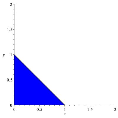
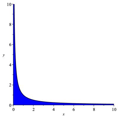
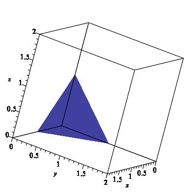
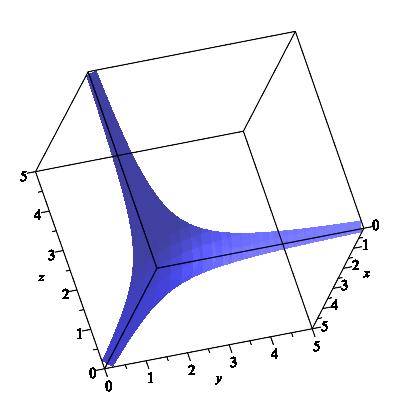
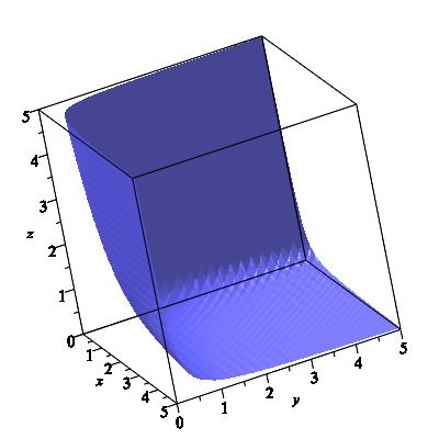
Figure 1. Hyperbolic regions defined by (2.2) with $c=1$. The first row: $\mathcal{H}_{1,2}(1)$ and $\mathcal{H}_{2,2}(1)$. The second row: $\mathcal{H}_{1,3}(1)$, $\mathcal{H}_{2,3}(1)$ and $\mathcal{H}_{3,3}(1)$. The adjective ‘hyperbolic’ stems from the fact that, for $r\geqslant 2$ and $1<\ell\leqslant r$, the set $\{(x_{1},x_{2})\in\mathbb{R}^{2}_{\geqslant 0}:P_{\ell}(x_{1},x_{2},c_{3},\ldots,c_{r})=c\}$ defines either a hyperbola or an empty set for all $c_{3},\ldots,c_{r}>0$ and $c>0$. This term is not quite appropriate in the case $\ell=1$, in which $\mathcal{H}_{1,r}(c)$ is an $r$-dimensional polytope.

For an arithmetic function $f:\mathbb{N}\to\mathbb{C}$ and $n\geqslant\binom{r}{\ell}$, consider the random variables

$$f_{\ell,r,G}(n):=f({\rm GCD}\,(V_{1}^{(n)},V_{2}^{(n)},\ldots,V_{r}^{(n)}))~{}\text{and}~{}f_{\ell,r,L}(n):=f({\rm LCM}\,(V_{1}^{(n)},V_{2}^{(n)},\ldots,V_{r}^{(n)})).$$ (2.3)

The following equalities extend formula (1.3):

$$\mathbb{E}f_{\ell,r,G}(n) =\frac{1}{|H_{\ell,r}(n)|}\sum_{(i_{1},\ldots,i_{r})\in H_{\ell,r}(n)}f({\rm GCD}\,(i_{1},i_{2},\ldots,i_{r})),$$

$$\mathbb{E}f_{\ell,r,L}(n) =\frac{1}{|H_{\ell,r}(n)|}\sum_{(i_{1},\ldots,i_{r})\in H_{\ell,r}(n)}f({\rm LCM}\,(i_{1},i_{2},\ldots,i_{r})).$$

Thus, deriving the asymptotics of the hyperbolic sums $\sum_{(i_{1},\ldots,i_{r})\in H_{\ell,r}(n)}f({\rm GCD}\,(i_{1},i_{2},\ldots,i_{r}))$ and $\sum_{(i_{1},\ldots,i_{r})\in H_{\ell,r}(n)}f({\rm LCM}\,(i_{1},i_{2},\ldots,i_{r}))$ is equivalent to finding the asymptotics of the counting function $|H_{\ell,r}(n)|$ and the expectations $\mathbb{E}f_{\ell,r,G}(n)$ and $\mathbb{E}f_{\ell,r,L}(n)$, respectively. The latter will be obtained for various functions $f$ from the corresponding distributional limit theorems for

$${\rm GCD}\,(V_{1}^{(n)},V_{2}^{(n)},\ldots,V_{r}^{(n)})\quad\text{and}\quad{\rm LCM}\,(V_{1}^{(n)},V_{2}^{(n)},\ldots,V_{r}^{(n)}).$$

3. Statement of the main results

3.1. First properties of the uniform distribution on $H_{\ell,r}(n)$

We start with some basic asymptotic properties of the distribution of $(V_{1}^{(n)},V_{2}^{(n)},\ldots,V_{r}^{(n)})$, which, we recall, is the uniform distribution on the set $H_{\ell,r}(n)$ defined in (2.1).

Proposition 3.1.

Assume that $r\geqslant 2$ and $1\leqslant\ell<r$. Then, for $\alpha_{1},\ldots,\alpha_{r}>0$,

$$\lim_{n\to\infty}\mathbb{P}\left\{V_{1}^{(n)}\leqslant\alpha_{1}n^{1/\ell},\ldots,V_{r}^{(n)}\leqslant\alpha_{r}n^{1/\ell}\right\}=\frac{1}{\mathcal{V}_{\ell,r}}\int_{0}^{\alpha_{1}}\cdots\int_{0}^{\alpha_{r}}\mathbbm{1}_{\{P_{\ell}(y_{1},y_{2},\ldots,y_{r})\leqslant 1\}}{\rm d}y_{1}\cdots{\rm d}y_{r}.$$

Proposition 3.1, as well as all subsequent results stated in this section, will be proved in Section 4.

In the case $r=\ell$, the limit relation is of different nature, for the volume $\mathcal{V}_{r,r}$ is infinite. In the sequel, we find it more convenient to write distributional limit relations using ‘$\overset{{\rm d}}{\underset{n\to\infty}{\longrightarrow}}$’ notation. Specifically, for fixed $r\in\mathbb{N}$, the notation

$$(X_{n,1},\ldots,X_{n,r})\overset{{\rm d}}{\underset{n\to\infty}{\longrightarrow}}(X_{1},\ldots,X_{r})$$

means that $\mathbb{P}\{X_{n,1}\leqslant x_{1},\ldots,X_{n,r}\leqslant x_{r}\}\to\mathbb{P}\{X_{1}\leqslant x_{1},\ldots,X_{r}\leqslant x_{r}\}$, as $n\to\infty$, for each continuity point $(x_{1},\ldots,x_{r})$ of the distribution function $(y_{1},\ldots,y_{r})\mapsto\mathbb{P}\{X_{1}\leqslant y_{1},\ldots,X_{r}\leqslant y_{r}\}$.

Let $Z_{1},\ldots,Z_{r-1}$ be independent random variables with continuous uniform distribution on $[0,1]$. Denote by $Z^{(1)}<Z^{(2)}<\ldots<Z^{(r-1)}$ their order statistics. Put $Z^{(r)}:=1$,

$$J_{1}:=Z^{(1)}\quad\text{and}\quad J_{k}=Z^{(k)}-Z^{(k-1)},\quad k=2,\ldots,r.$$

Proposition 3.2.

Assume that $r=\ell\geqslant 2$. Then

$$\left(\frac{\log V_{1}^{(n)}}{\log n},\frac{\log V_{2}^{(n)}}{\log n},\ldots,\frac{\log V_{r}^{(n)}}{\log n}\right)\overset{{\rm d}}{\underset{n\to\infty}{\longrightarrow}}\left(J_{1},J_{2},\ldots,J_{r}\right),$$ (3.1)

or, equivalently,

$$\left(\frac{\log V_{1}^{(n)}}{\log n},\frac{\log(V_{1}^{(n)}V_{2}^{(n)})}{\log n},\ldots,\frac{\log(V_{1}^{(n)}\cdots V_{r}^{(n)})}{\log n}\right)\overset{{\rm d}}{\underset{n\to\infty}{\longrightarrow}}\left(Z^{(1)},Z^{(2)},\ldots,Z^{(r)}\right).$$ (3.2)

The next result deals with limit theorems for the product $V_{1}^{(n)}V_{2}^{(n)}\cdots V_{r}^{(n)}$.

Proposition 3.3.

Assume that $r=\ell\geqslant 2$. Then

$$\frac{V_{1}^{(n)}V_{2}^{(n)}\cdots V_{r}^{(n)}}{n}\overset{{\rm d}}{\underset{n\to\infty}{\longrightarrow}}U_{r,r},$$ (3.3)

where $U_{r,r}$ has a continuous uniform distribution on $[0,1]$.

Assume that $1\leqslant\ell<r$. Then

$$\frac{V_{1}^{(n)}V_{2}^{(n)}\cdots V_{r}^{(n)}}{n^{r/\ell}}\overset{{\rm d}}{\underset{n\to\infty}{\longrightarrow}}U_{\ell,r},$$ (3.4)

where $U_{\ell,r}$ has the distribution function

$$\mathbb{P}\{U_{\ell,r}\leqslant x\}=\frac{1}{\mathcal{V}_{\ell,r}}\int_{0}^{\infty}\cdots\int_{0}^{\infty}\mathbbm{1}_{\{P_{\ell}(y_{1},y_{2},\ldots,y_{r})\leqslant 1,\;y_{1}y_{2}\cdots y_{r}\leqslant x\}}{\rm d}y_{1}\cdots{\rm d}y_{r},\quad x\in\left[0,\,x^{\ast}_{\ell,r}\right],$$ (3.5)

and $x^{\ast}_{\ell,r}:=\binom{r}{\ell}^{-r/\ell}$.

In both cases, for $n\geqslant\binom{r}{\ell}$ (with $\ell=r$ in the first case),

$$\mathbb{P}\left\{0\leqslant\frac{V_{1}^{(n)}V_{2}^{(n)}\cdots V_{r}^{(n)}}{n^{r/\ell}}\leqslant 1\right\}=1.$$ (3.6)

In particular, all power moments of positive orders in relations (3.3) and (3.4) converge to the corresponding moments of the limit random variables.

Example 3.4.

The distribution function of $U_{1,2}$ can be explicitly calculated and takes the following form:

$$\mathbb{P}\{U_{1,2}\leqslant x\}=1-\sqrt{1-4x}+2x\log\left(\frac{1+\sqrt{1-4x}}{1-\sqrt{1-4x}}\right),\quad x\in[0,\,1/4],$$

with a density (the derivative) $x\mapsto 2\log\left(\frac{1+\sqrt{1-4x}}{1-\sqrt{1-4x}}\right)\mathbbm{1}_{[0,\,1/4]}(x)$. For other values of $\ell<r$, there seems to be no simple closed form expression for $\mathbb{P}\{U_{\ell,r}\leqslant x\}$.

3.2. Arithmetic properties of the uniform distribution on $H_{\ell,r}(n)$

Our next result shows that without any assumptions on the function $f$, the random variables $f_{\ell,r,G}(n)$ in (2.3) converge in distribution, as $n\to\infty$.

As a preparation, we introduce a collection of random variables, which is of major importance for the subsequent analysis. Let $\mathcal{P}$ denote the set of prime numbers and $(\mathcal{G}_{k}(p))_{k\in\mathbb{N},p\in\mathcal{P}}$ be a collection of mutually independent random variables with the following geometric distributions

$$\mathbb{P}\{\mathcal{G}_{k}(p)=j\}=\left(1-\frac{1}{p}\right)\frac{1}{p^{j}},\quad j=0,1,2,\ldots$$

Finally, let $\lambda_{p}(n)\in\{0,1,2,\ldots\}$ denote the multiplicity of a prime $p$ in the prime decomposition of an integer $n$, that is,

$$n=\prod_{p\in\mathcal{P}}p^{\lambda_{p}(n)}.$$

Theorem 3.5.

Let $f:\mathbb{N}\to\mathbb{C}$ be an arithmetic function. Then

$$f_{\ell,r,G}(n)\overset{{\rm d}}{\underset{n\to\infty}{\longrightarrow}}f\left(\prod_{p\in\mathcal{P}}p^{\min_{k=1,\ldots,r}\mathcal{G}_{k}(p)}\right).$$ (3.7)

Remark 3.6.

The distribution of the random variable

$$U^{(r,\infty)}:=\prod_{p\in\mathcal{P}}p^{\min_{k=1,\ldots,r}\mathcal{G}_{k}(p)}$$

can be characterized as follows. Since the minimum of independent geometric variables has again a geometric distribution with the parameter being the product of the parameters of individual variables, the Mellin transform of $U^{(r,\infty)}$ is given by

$$\mathbb{E}\bigl{(}(U^{(r,\infty)})^{s}\bigr{)}=\prod_{p\in\mathcal{P}}\mathbb{E}p^{s\min_{k=1,\ldots,r}\mathcal{G}_{k}(p)}=\prod_{p\in\mathcal{P}}\left(\sum_{j=0}^{\infty}p^{sj}\left(1-\frac{1}{p^{r}}\right)\frac{1}{p^{rj}}\right)=\frac{\zeta(r-s)}{\zeta(r)},\quad s<r-1.$$

We have used Euler’s product formula for the last equality.

Theorem 3.7 below is a limit theorem for the ${\rm LCM}\,$.

Theorem 3.7.

The following convergence in distribution holds true:

$$\frac{{\rm LCM}\,(V_{1}^{(n)},V_{2}^{(n)},\ldots,V_{r}^{(n)})}{V_{1}^{(n)}V_{2}^{(n)}\cdots V_{r}^{(n)}} \overset{{\rm d}}{\underset{n\to\infty}{\longrightarrow}}\prod_{p\in\mathcal{P}}p^{\max_{k=1,\ldots,r}\mathcal{G}_{k}(p)-\sum_{k=1}^{r}\mathcal{G}_{k}(p)},\vskip 6.0pt plus 2.0pt minus 2.0pt$$ (3.8)

$$\frac{{\rm LCM}\,(V_{1}^{(n)},V_{2}^{(n)},\ldots,V_{r}^{(n)})}{n^{r/\ell}} \overset{{\rm d}}{\underset{n\to\infty}{\longrightarrow}}U_{\ell,r}\prod_{p\in\mathcal{P}}p^{\max_{k=1,\ldots,r}\mathcal{G}_{k}(p)-\sum_{k=1}^{r}\mathcal{G}_{k}(p)},$$ (3.9)

where the random variable $U_{\ell,r}$ on the right-hand side of (3.9) is independent of the $\mathcal{G}_{k}(p)$ and has the distribution given by (3.5) if $\ell<r$, and has the uniform distribution on $[0,1]$ if $\ell=r$. Moreover, in both relations (3.8) and (3.9), all power moments of positive orders converge to the corresponding moments of the limit random variables.

Our last result is concerned with the asymptotic behavior of the average $\mathbb{E}f_{\ell,r,L}(n)$. Recall that a real-valued measurable function $f$ defined in a neighbourhood of $+\infty$ is called regularly varying at $\infty$ if there exists $\beta\in\mathbb{R}$ such that, for all $\lambda>0$,

$$\lim_{t\to\infty}\frac{f(\lambda t)}{f(t)}=\lambda^{\beta}.$$

The parameter $\beta$ is called the index of regular variation of $f$ at $\infty$. We refer to [3] for a comprehensive information on regularly varying functions.

Corollary 3.8.

Let $f:\mathbb{R}^{r}_{\geqslant 0}\to\mathbb{R}$ be a locally bounded function which varies regularly at $\infty$ of index $\beta>0$. Then, as $n\to\infty$,

$$\mathbb{E}f_{\ell,r,L}(n)=\frac{1}{|H_{\ell,r}(n)|}\sum_{(i_{1},\ldots,i_{r})\in H_{\ell,r}(n)}f({\rm LCM}\,(i_{1},i_{2},\ldots,i_{r}))\\ \sim~{}\mathbb{E}(U_{\ell,r}^{\beta})\mathbb{E}\left(\biggl{(}\prod_{p\in\mathcal{P}}p^{\max_{k=1,\ldots,r}\mathcal{G}_{k}(p)-\sum_{k=1}^{r}\mathcal{G}_{k}(p)}\biggr{)}^{\beta}\right)f(n^{r/\ell}).$$

4. Proofs of the main results

We start with the detailed analysis of the counting functions $|H_{\ell,r}(n)|$, which is an essential ingredient for the proofs of our main results.

4.1. Properties of the counting function when $\ell=1$ and $\ell=r$.

We first consider the case $\ell=1$ and $r\in\mathbb{N}$. Then

$$H_{1,r}(n)=\{(i_{1},\ldots,i_{r})\in\mathbb{N}^{r}:i_{1}+i_{2}+\cdots+i_{r}\leqslant n\},$$

and there is the obvious exact formula $|H_{1,r}(n)|=\binom{n}{r}$, which entails that, as $n\to\infty$,

$$|H_{1,r}(n)|~{}\sim~{}\frac{n^{r}}{r!}.$$ (4.1)

Assume now that $r=\ell\geqslant 2$. Then

$$H_{r,r}(n)=\{(i_{1},\ldots,i_{r})\in\mathbb{N}^{r}:i_{1}i_{2}\cdots i_{r}\leqslant n\}.$$

Although there is no simple exact formula for the cardinality of $H_{r,r}(n)$, one can easily derive the exact growth rate of $|H_{r,r}(n)|$. This is given in the next proposition.

Proposition 4.1.

For fixed $r\geqslant 2$, as $n\to\infty$,

$$|H_{r,r}(n)|=\frac{n\log^{r-1}n}{(r-1)!}+O(n\log^{r-2}n).$$

Proof.

Put $W_{r}(n):=|H_{r,r}(n)|$. Then $W_{1}(n)=n$ and

$$W_{r}(n)=\sum_{i=1}^{n}W_{r-1}\left(\left\lfloor\frac{n}{i}\right\rfloor\right),\quad r\geqslant 2.$$ (4.2)

The claim of Proposition 4.1 follows by induction on $r$ with the help of the asymptotic relation

$$\sum_{i=1}^{n}\left\lfloor\frac{n}{i}\right\rfloor\log^{k-1}\left(\left\lfloor\frac{n}{i}\right\rfloor\right)=\sum_{i=1}^{n}\frac{n}{i}\log^{k-1}\left(\frac{n}{i}\right)+O(n\log^{k-1}n)=\frac{n\log^{k}n}{k}+O(n\log^{k-1}n),\quad n\to\infty,$$

which holds for every fixed $k\in\mathbb{N}$. ∎

Corollary 4.2.

For fixed $r\in\mathbb{N}$, the sequence $(|H_{r,r}(n)|)_{n\in\mathbb{N}}$ is regularly varying at $\infty$ of index $1$, that is, for each $\lambda>0$,

$$\lim_{n\to\infty}\frac{|H_{r,r}(\lfloor\lambda n\rfloor)|}{|H_{r,r}(n)|}=\lambda.$$

The result of Corollary 4.2 is less precise than that of Proposition 4.1. It is stated here only for comparison to its counterpart, Corollary 4.5, which treats the case $1<\ell<r$.

4.2. Properties of the counting function when $1<\ell<r$.

Comparing (4.1) and Proposition 4.1 and keeping in mind the homogeneity properties of $P_{\ell}$, one could think that the asymptotics of $|H_{\ell,r}(n)|$ in the intermediate regimes should be of the form $C_{r}n^{r/\ell}\log^{\ell-1}n$. This, however, turns out to be wrong in that there is no logarithmic factor, that is, the correct answer is $|H_{\ell,r}(n)|\sim C_{r}n^{r/\ell}$ for an appropriate $C_{r}>0$. This is, in fact, a consequence of the finiteness of the volumes $\mathcal{V}_{\ell,r}$ for $\ell<r$.

Lemma 4.3.

For all $r\geqslant 2$ and $1\leqslant\ell<r$, ${\bf Vol}\,(\mathcal{H}_{\ell,r}(c))=c^{r/\ell}{\bf Vol}\,(\mathcal{H}_{\ell,r}(1))<\infty$.

Proof.

We proceed in two steps. First, we show that

$${\bf Vol}\,(\mathcal{H}_{r-1,r}(1))<\infty.$$ (4.3)

As a second step, we prove that

$$\mathcal{H}_{\ell,r}(1)\subseteq\mathcal{H}_{r-1,r}(r),\quad\ell<r.$$ (4.4)

To check (4.3), observe that

$${\bf Vol}\,(\mathcal{H}_{r-1,r}(1))=\int_{0}^{\infty}\cdots\int_{0}^{\infty}\mathbbm{1}_{\{P_{r-1}(y_{1},y_{2},\ldots,y_{r})\leqslant 1\}}{\rm d}y_{1}\cdots{\rm d}y_{r}.$$

Changing the variables $z_{j}:=(y_{1}y_{2}\cdots y_{r})/y_{j}$ or, equivalently, $y_{j}=(z_{1}z_{2}\cdots z_{r})^{1/(r-1)}z_{j}^{-1}$, $j=1,\ldots,r$, we conclude that the partial derivatives are given by

$$\frac{\partial y_{j}}{\partial z_{k}}=\begin{cases}(r-1)^{-1}(z_{1}z_{2}\cdots z_{r})^{1/(r-1)}z_{j}^{-1}z_{k}^{-1},&j\neq k,\\ \frac{2-r}{r-1}(z_{1}z_{2}\cdots z_{r})^{1/(r-1)}z_{j}^{-2},&j=k.\\ \end{cases}$$

Thus, the Jacobian determinant $J$ is equal to

$$J=(z_{1}z_{2}\cdots z_{r})^{\frac{r}{r-1}}\left|\begin{matrix}\frac{2-r}{r-1}\frac{1}{z_{1}^{2}}&\frac{1}{r-1}\frac{1}{z_{1}z_{2}}&\cdots&\frac{1}{r-1}\frac{1}{z_{1}z_{r}}\\ \frac{1}{r-1}\frac{1}{z_{2}z_{1}}&\frac{2-r}{r-1}\frac{1}{z_{2}^{2}}&\cdots&\frac{1}{r-1}\frac{1}{z_{2}z_{r}}\\ \vdots&\vdots&\ddots&\vdots\\ \frac{1}{r-1}\frac{1}{z_{r}z_{1}}&\frac{1}{r-1}\frac{1}{z_{r}z_{2}}&\cdots&\frac{2-r}{r-1}\frac{1}{z_{r}^{2}}\end{matrix}\right|=\frac{1}{(z_{1}z_{2}\cdots z_{r})^{\frac{r-2}{r-1}}}\left|\begin{matrix}\frac{2-r}{r-1}&\frac{1}{r-1}&\cdots&\frac{1}{r-1}\\ \frac{1}{r-1}&\frac{2-r}{r-1}&\cdots&\frac{1}{r-1}\\ \vdots&\vdots&\ddots&\vdots\\ \frac{1}{r-1}&\frac{1}{r-1}&\cdots&\frac{2-r}{r-1}\end{matrix}\right|\\ =\frac{(-1)^{r-1}}{(r-1)(z_{1}z_{2}\cdots z_{r})^{\frac{r-2}{r-1}}},$$

whence

$${\bf Vol}\,(\mathcal{H}_{r-1,r}(1))=\frac{1}{r-1}\int_{0}^{\infty}\cdots\int_{0}^{\infty}\frac{\mathbbm{1}_{\{z_{1}+z_{2}+\cdots+z_{r}\leqslant 1\}}}{(z_{1}z_{2}\cdots z_{r})^{\frac{r-2}{r-1}}}{\rm d}z_{1}\cdots{\rm d}z_{r}\\ \leqslant\frac{1}{r-1}\int_{0}^{1}\cdots\int_{0}^{1}\frac{1}{(z_{1}z_{2}\cdots z_{r})^{\frac{r-2}{r-1}}}{\rm d}z_{1}\cdots{\rm d}z_{r}=(r-1)^{r-1}<\infty.$$

This proves (4.3).

Turning to (4.4), pick $(x_{1},x_{2},\ldots,x_{r})\in\mathcal{H}_{\ell,r}(1)$. Then

$$x_{i_{1}}x_{i_{2}}\cdots x_{i_{\ell}}\leqslant 1,\quad\text{ for every }\ell\text{-tuple}\quad 1\leqslant i_{1}<i_{2}<\cdots<i_{\ell}\leqslant r.$$

Fix $k=1,\ldots,r$ and multiply the above inequalities over all $\ell$-tuples taken from $\{1,2,\ldots,k-1,k+1,\ldots,r\}$. This yields $x_{1}x_{2}\cdots x_{k-1}x_{k+1}\cdots x_{r}\leqslant 1$ and thereupon $P_{r-1}(x_{1},x_{2},\ldots,x_{r})\leqslant r$, meaning that $(x_{1},x_{2},\ldots,x_{r})\in\mathcal{H}_{r-1,r}(r)$. ∎

Proposition 4.4.

For fixed $r\geqslant 2$ and $\ell<r$,

$$\lim_{n\to\infty}\frac{|H_{\ell,r}(n)|}{n^{r/\ell}}=\mathcal{V}_{\ell,r}.$$

Proof.

By homogeneity of $P_{\ell}$,

$$\frac{|H_{\ell,r}(n)|}{n^{r/\ell}}=\frac{1}{n^{r/\ell}}\sum_{i_{1}=1}^{\infty}\cdots\sum_{i_{r}=1}^{\infty}\mathbbm{1}_{\{P_{\ell}(i_{1},\ldots,i_{r})\leqslant n\}}=\frac{1}{(n^{1/\ell})^{r}}\sum_{i_{1}=1}^{\infty}\cdots\sum_{i_{r}=1}^{\infty}\mathbbm{1}_{\{P_{\ell}(i_{1}/n^{1/\ell},\ldots,i_{r}/n^{1/\ell})\leqslant 1\}}.$$

The claim follows from Proposition A.1 (see Appendix A) applied to the function $g(y_{1},\ldots,y_{r}):=\mathbbm{1}_{\{P_{\ell}(y_{1},\ldots,y_{r})\leqslant 1\}}$. Indeed, while this function is obviously coordinatewise nonincreasing, its integrability follows from Lemma 4.3. ∎

Corollary 4.5.

For fixed $r\geqslant 2$ and $1\leqslant\ell<r$, the sequence $(|H_{\ell,r}(n)|)_{n\geqslant\binom{r}{\ell}}$ is regularly varying at $\infty$ of index $r/\ell$, that is, for each $\lambda>0$,

$$\lim_{n\to\infty}\frac{|H_{\ell,r}(\lfloor n\lambda\rfloor)|}{|H_{\ell,r}(n)|}=\lambda^{r/\ell}.$$

Proposition 4.6.

For fixed $r\geqslant 2$, $1\leqslant\ell\leqslant r$ and $t_{1},\ldots,t_{r}>0$,

$$\lim_{n\to\infty}\frac{|\{(i_{1},\ldots,i_{r})\in\mathbb{N}^{r}:P_{\ell}(t_{1}i_{1},\ldots,t_{r}i_{r})\leqslant n\}|}{|H_{\ell,r}(n)|}=\left(\prod_{k=1}^{r}t_{k}\right)^{-1}.$$

Proof.

If $\ell=r$, the claim immediately follows from Corollary 4.2, because

$$|\{(i_{1},\ldots,i_{r})\in\mathbb{N}^{r}:P_{r}(t_{1}i_{1},\ldots,t_{r}i_{r})\leqslant n\}|\\ =|\{(i_{1},\ldots,i_{r})\in\mathbb{N}^{r}:t_{1}i_{1}\cdots t_{r}i_{r}\leqslant n\}|=\left|H_{r,r}\left(\left\lfloor\frac{n}{t_{1}t_{2}\cdots t_{r}}\right\rfloor\right)\right|.$$

From now on, we assume that $\ell<r$. Write

$$|\{(i_{1},\ldots,i_{r})\in\mathbb{N}^{r}:P_{\ell}(t_{1}i_{1},\ldots,t_{r}i_{r})\leqslant n\}| =\sum_{i_{1}=1}^{\infty}\cdots\sum_{i_{r}=1}^{\infty}\mathbbm{1}_{\{P_{\ell}(t_{1}i_{1},\ldots,t_{r}i_{r})\leqslant n\}}$$

$$=\sum_{i_{1}=1}^{\infty}\cdots\sum_{i_{r}=1}^{\infty}\mathbbm{1}_{\{P_{\ell}(t_{1}i_{1}/n^{1/\ell},\ldots,t_{r}i_{r}/n^{1/\ell})\leqslant 1\}}.$$

Applying Proposition A.1 with the function $g(y_{1},\ldots,y_{r}):=\mathbbm{1}_{\{P_{\ell}(t_{1}y_{1},\ldots,t_{r}y_{r})\leqslant 1\}}$ and using Proposition 4.4, we infer

$$\lim_{n\to\infty}\frac{|\{(i_{1},\ldots,i_{r})\in\mathbb{N}^{r}:P_{\ell}(t_{1}i_{1},\ldots,t_{r}i_{r})\leqslant n\}|}{|H_{\ell,r}(n)|}\\ =\frac{1}{\mathcal{V}_{\ell,r}}\int_{0}^{\infty}\cdots\int_{0}^{\infty}\mathbbm{1}_{\{P_{\ell}(t_{1}y_{1},\ldots,t_{r}y_{r})\leqslant 1\}}{\rm d}y_{1}\cdots{\rm d}y_{r}=\left(\prod_{k=1}^{r}t_{k}\right)^{-1}.$$

For future use, we note here that

$$|\{(i_{1},\ldots,i_{r})\in\mathbb{N}^{r}:P_{\ell}(t_{1}i_{1},\ldots,t_{r}i_{r})\leqslant n\}|\leqslant\frac{n^{r/\ell}\mathcal{V}_{\ell,r}}{t_{1}t_{2}\cdots t_{r}},\quad 1\leqslant\ell<r,$$ (4.5)

which is a direct consequence of monotonicity. ∎

4.3. Proofs of Propositions 3.1, 3.2 and 3.3

Proof of Proposition 3.1.

The proof again relies on Proposition A.1 from the Appendix. Note that

$$\mathbb{P} \left\{V_{1}^{(n)}\leqslant\alpha_{1}n^{1/\ell},\ldots,V_{r}^{(n)}\leqslant\alpha_{r}n^{1/\ell}\right\}$$

$$=\frac{|\{(i_{1},\ldots,i_{r})\in\mathbb{N}^{r}:P_{\ell}(i_{1},\ldots,i_{r})\leqslant n,i_{1}\leqslant\alpha_{1}n^{1/\ell},\ldots,i_{r}\leqslant\alpha_{r}n^{1/\ell}\}|}{|H_{\ell,r}(n)|}$$

$$=\frac{n^{-r/\ell}|\{(i_{1},\ldots,i_{r})\in\mathbb{N}^{r}:P_{\ell}(i_{1}/n^{1/\ell},\ldots,i_{r}/n^{1/\ell})\leqslant 1,i_{1}/n^{1/\ell}\leqslant\alpha_{1},\ldots,i_{r}/n^{1/\ell}\leqslant\alpha_{r}\}|}{n^{-r/\ell}|H_{\ell,r}(n)|},$$

and the right-hand side converges, as $n\to\infty$, to

$$\frac{1}{\mathcal{V}_{\ell,r}}\int_{0}^{\alpha_{1}}\cdots\int_{0}^{\alpha_{r}}\mathbbm{1}_{\{P_{\ell}(y_{1},y_{2},\ldots,y_{r})\leqslant 1\}}{\rm d}y_{1}\cdots{\rm d}y_{r}.\qed$$

We first prove Proposition 3.3, for this result will be used in the proof of Proposition 3.2.

Proof of Proposition 3.3.

For a proof of (3.3), note that, for $x\in[0,\,1]$ and $n\in\mathbb{N}$,

$$\mathbb{P}\{V_{1}^{(n)}V_{2}^{(n)}\cdots V_{r}^{(n)}\leqslant xn\}=\frac{|\{(i_{1},\ldots,i_{r})\in\mathbb{N}^{r}:i_{1}i_{2}\cdots i_{r}\leqslant xn\}|}{|\{(i_{1},\ldots,i_{r})\in\mathbb{N}^{r}:i_{1}i_{2}\cdots i_{r}\leqslant n\}|},$$ (4.6)

which, in view of Corollary 4.2, converges to $x$, as $n\to\infty$. As for (3.4), write

$$\mathbb{P}\{V_{1}^{(n)}V_{2}^{(n)}\cdots V_{r}^{(n)}\leqslant xn^{r/\ell}\}=\frac{|\{(i_{1},\ldots,i_{r})\in\mathbb{N}^{r}:P_{\ell}(i_{1},\ldots,i_{r})\leqslant n,i_{1}\cdots i_{r}\leqslant xn^{r/\ell}\}|}{|H_{\ell,r}(n)|}\\ =\frac{n^{-r/\ell}|\{(i_{1},\ldots,i_{r})\in\mathbb{N}^{r}:P_{\ell}(i_{1}/n^{1/\ell},\ldots,i_{r}/n^{1/\ell})\leqslant 1,(i_{1}/n^{1/\ell})\cdots(i_{r}/n^{1/\ell})\leqslant x\}|}{n^{-r/\ell}|H_{\ell,r}(n)|}.$$

While the numerator converges to the integral on the right-hand side of (3.5), by Proposition A.1 applied with $g(y_{1},\ldots,y_{r})=\mathbbm{1}_{\{P_{\ell}(y_{1},\ldots,y_{r})\leqslant 1,\;y_{1}\cdots y_{r}\leqslant x\}}$, the denominator converges to $\mathcal{V}_{\ell,r}$, by Proposition 4.4. The value $x^{\ast}_{\ell,r}$ in (3.5) is the supremum of the support of $U_{\ell,r}$. It can be found as the largest real number such that the surfaces $P_{\ell}(x_{1},\ldots,x_{r})=1$ and $x_{1}\cdots x_{r}=x^{\ast}_{\ell,r}$ have a nonempty intersection.

Formula (3.6) is obvious for $\ell=r$, since, by construction, $(V_{1}^{(n)},\ldots,V_{r}^{(n)})$ is a point chosen at random in the set $H_{r,r}(n)$. Alternatively, (3.6) follows on putting $x=1$ in (4.6). If $\ell<r$, formula (3.6) can be proved as follows. By definition, $P_{\ell}(V_{1}^{(n)},\ldots,V_{r}^{(n)})\leqslant n$, which implies

$$\mathbb{P}\left\{\frac{V_{i_{1}}^{(n)}}{n^{1/\ell}}\frac{V_{i_{2}}^{(n)}}{n^{1/\ell}}\cdots\frac{V_{i_{\ell}}^{(n)}}{n^{1/\ell}}\leqslant 1\right\}=1,$$

for all $\ell$-tuples taken from $\{1,2,\ldots,r\}$. Multiplying all these inequalities, we obtain (3.6). ∎

Proof of Proposition 3.2.

We first observe that (3.3) implies

$$\lim_{n\to\infty}\mathbb{P}\left\{V_{1}^{(n)}\cdots V_{r}^{(n)}\leqslant n^{\beta}\right\}=0,$$ (4.7)

for every fixed $\beta<1$.

We shall prove a relation equivalent to (3.2), namely, for all $0<\beta_{1}<\ldots<\beta_{r-1}<\beta_{r}<1$ and sufficiently small $h_{1},\ldots,h_{r-1},h_{r}>0$ such that the intervals

$$(\beta_{1},\beta_{1}+h_{1}],(\beta_{2},\beta_{2}+h_{2}],\ldots,(\beta_{r-1},\beta_{r-1}+h_{r-1}],(\beta_{r},\beta_{r}+h_{r}]$$

are disjoint,

$$\lim_{n\to\infty}\mathbb{P}\{V_{1}^{(n)}\in(n^{\beta_{1}},n^{\beta_{1}+h_{1}}],V_{1}^{(n)}V_{2}^{(n)}\in(n^{\beta_{2}},n^{\beta_{2}+h_{2}}],\ldots,V_{1}^{(n)}V_{2}^{(n)}\cdots V_{r}^{(n)}\in(n^{\beta_{r}},n^{\beta_{r}+h_{r}}]\}\\ =\mathbb{P}\{Z^{(1)}\in(\beta_{1},\beta_{1}+h_{1}],Z^{(2)}\in(\beta_{2},\beta_{2}+h_{2}],\ldots,Z^{(r)}\in(\beta_{r},\beta_{r}+h_{r}]\}\\ =(r-1)!h_{1}\cdots h_{r-1}\mathbbm{1}_{\{\beta_{r}+h_{r}\geqslant 1\}}.\hskip 215.10284pt$$ (4.8)

The second equality in (4.8) follows from the fact that $(Z^{(1)},\ldots,Z^{(r-1)})$ has a constant density in the region $\{(x_{1},\ldots,x_{r-1})\in[0,1]^{r-1}:x_{1}\leqslant\cdots\leqslant x_{r-1}\leqslant 1\}$, which is equal to $(r-1)!$, see, for instance, formula (1.4) on p. 238 in [8]. An appeal to (4.7) and the fact that $V_{1}^{(n)}V_{2}^{(n)}\cdots V_{r}^{(n)}\leqslant n$ justifies the equivalence of (4.8) and

$$\lim_{n\to\infty}\mathbb{P}\{V_{1}^{(n)}\in(n^{\beta_{1}},n^{\beta_{1}+h_{1}}],V_{1}^{(n)}V_{2}^{(n)}\in(n^{\beta_{2}},n^{\beta_{2}+h_{2}}],\ldots,V_{1}^{(n)}V_{2}^{(n)}\cdots V_{r-1}^{(n)}\in(n^{\beta_{r-1}},n^{\beta_{r-1}+h_{r-1}}]\}\\ =(r-1)!h_{1}\cdots h_{r-1}.$$ (4.9)

The probability on the left-hand side of (4.9) is equal to

$$\frac{|\{(i_{1},\ldots,i_{r}):i_{1}\in(n^{\beta_{1}},n^{\beta_{1}+h_{1}}],\ldots,i_{1}\cdots i_{r-1}\in(n^{\beta_{r-1}},n^{\beta_{r-1}+h_{r-1}}],i_{1}\cdots i_{r}\leqslant n\}|}{|H_{r,r}(n)|}.$$

Hence, according to Proposition 4.1, formula (4.9) follows once we can check that the numerator is asymptotically equivalent to $h_{1}\cdots h_{r-1}n\log^{r-1}n$, as $n\to\infty$. The latter relation can be written as

$$\sum_{i_{1}=1}^{\infty}\mathbbm{1}_{\{i_{1}\in(n^{\beta_{1}},n^{\beta_{1}+h_{1}}]\}}\sum_{i_{2}=1}^{\infty}\mathbbm{1}_{\{i_{2}\in(n^{\beta_{2}}/i_{1},n^{\beta_{2}+h_{2}}/i_{1}]\}}\cdots\sum_{i_{r-1}=1}^{\infty}\mathbbm{1}_{\{i_{r-1}\in(n^{\beta_{r-1}}/(i_{1}\cdots i_{r-2}),n^{\beta_{r-1}+h_{r-1}}/(i_{1}\cdots i_{r-2})]\}}\\ \sum_{i_{r}=1}^{\infty}\mathbbm{1}_{\{i_{r}\leqslant n/(i_{1}\cdot\ldots\cdot i_{r-1})\}}~{}\sim~{}h_{1}\cdots h_{r-1}n\log^{r-1}n,$$

or after calculating the rightmost sum as

$$\sum_{i_{1}=1}^{\infty}\frac{\mathbbm{1}_{\{i_{1}\in(n^{\beta_{1}},n^{\beta_{1}+h_{1}}]\}}}{i_{1}}\sum_{i_{2}=1}^{\infty}\frac{\mathbbm{1}_{\{i_{2}\in(n^{\beta_{2}}/i_{1},n^{\beta_{2}+h_{2}}/i_{1}]\}}}{i_{2}}\cdots\sum_{i_{r-1}=1}^{\infty}\frac{\mathbbm{1}_{\{i_{r-1}\in(n^{\beta_{r-1}}/(i_{1}\cdots i_{r-2}),n^{\beta_{r-1}+h_{r-1}}/(i_{1}\cdots i_{r-2})]\}}}{i_{r-1}}\\ ~{}\sim~{}h_{1}\cdots h_{r-1}\log^{r-1}n.$$ (4.10)

Relation (4.10) readily follows by induction on $r\geqslant 2$ with the help of the formula

$$\sum_{i=1}^{\infty}\frac{\mathbbm{1}_{\{i\in[xn^{a},xn^{a+h}]\}}}{i}=h\log n+O(1),\quad n\to\infty,$$

which holds for all fixed $a,h>0$, uniformly in $x$ and $n$ satisfying $xn^{a}\to\infty$. In our setting, the latter relation is secured by $n^{\beta_{k-1}}/(i_{1}\cdots i_{k-2})\to\infty$ for every $k\geqslant 3$, which, in its turn, follows in view of $\beta_{k-2}+h_{k-2}<\beta_{k-1}$. ∎

4.4. Prime decomposition

The following proposition lies in the core of our main theorems and shows that as far as divisibility properties are concerned, the random vector $(V_{1}^{(n)},V_{2}^{(n)},\ldots,V_{r}^{(n)})$, uniformly distributed in the hyperbolic region $H_{\ell,r}(n)$, behaves as a set of $r$ independent variables uniformly distributed in $\{1,2,\ldots,n\}$, see, for example, Lemma 3.1 in [4].

Proposition 4.7.

Assume that $r\geqslant 2$. The following convergence in distribution holds true:

$$\left(\frac{V_{1}^{(n)}V_{2}^{(n)}\cdots V_{r}^{(n)}}{n^{r/\ell}},\left(\lambda_{p}(V_{1}^{(n)}),\ldots,\lambda_{p}(V_{r}^{(n)})\right)_{p\in\mathcal{P}}\right)\overset{{\rm d}}{\underset{n\to\infty}{\longrightarrow}}\left(U_{\ell,r},\left(\mathcal{G}_{1}(p),\ldots,\mathcal{G}_{r}(p)\right)_{p\in\mathcal{P}}\right)$$

on $\mathbb{R}\times(\mathbb{R}^{r})^{\infty}$, where $U_{\ell,r}$ on the right-hand side is independent of the $\mathcal{G}_{k}(p)$, for all $k=1,\ldots,r$ and $p\in\mathcal{P}$.

Proof.

Fix $m\in\mathbb{N}$, $x\geqslant 0$, pairwise distinct primes $p_{1},\ldots,p_{m}\in\mathcal{P}$ and arbitrary $j_{k,t}\in\{0,1,2,\ldots\}$ for $k=1,\ldots,r$ and $t=1,\ldots,m$. Write

$$\mathbb{P}\{V_{1}^{(n)}V_{2}^{(n)}\cdots V_{r}^{(n)}\leqslant xn^{r/\ell},\lambda_{p_{t}}(V_{k}^{(n)})\geqslant j_{k,t}\text{ for all }k=1,\ldots,r\text{ and }t=1,\ldots,m\}$$

$$=\mathbb{P}\{V_{1}^{(n)}V_{2}^{(n)}\cdots V_{r}^{(n)}\leqslant xn^{r/\ell},p_{t}^{j_{k,t}}\text{ divides }V_{k}^{(n)}\text{ for all }k=1,\ldots,r\text{ and }t=1,\ldots,m\}$$

$$=\frac{1}{|H_{\ell,r}(n)|}\sum_{i_{1}=1}^{\infty}\cdots\sum_{i_{r}=1}^{\infty}\mathbbm{1}\{P_{\ell}(i_{1},\ldots,i_{r})\leqslant n,i_{1}\cdots i_{r}\leqslant xn^{r/\ell},$$

$$\hskip 128.0374ptp_{t}^{j_{k,t}}\text{ divides }i_{k}\text{ for all }k=1,\ldots,r\text{ and }t=1,\ldots,m\}$$

$$=\frac{1}{|H_{\ell,r}(n)|}\sum_{i_{1}=1}^{\infty}\cdots\sum_{i_{r}=1}^{\infty}\mathbbm{1}\Big{\{}P_{\ell}(i_{1},\ldots,i_{r})\leqslant n,i_{1}\cdots i_{r}\leqslant xn^{r/\ell},$$

$$\hskip 128.0374pt\prod_{t=1}^{m}p_{t}^{j_{k,t}}\text{ divides }i_{k}\text{ for all }k=1,\ldots,r\Big{\}}.$$

For notational simplicity, put $\mu_{k}:=\prod_{t=1}^{m}p_{t}^{j_{k,t}}$. Since the sum over $i_{k}$ in the formula above is actually taken over multiples of $\mu_{k}$, $k=1,\ldots,r$, we obtain

$$\mathbb{P}\{V_{1}^{(n)}V_{2}^{(n)}\cdots V_{r}^{(n)}\leqslant xn^{\ell/r},\lambda_{p_{t}}(V_{k}^{(n)})\geqslant j_{k,t}\text{ for all }k=1,\ldots,r\text{ and }t=1,\ldots,m\}\\ =\frac{|\{(i_{1},\ldots,i_{r})\in\mathbb{N}^{r}:P_{\ell}(\mu_{1}i_{1},\ldots,\mu_{r}i_{r})\leqslant n,(\mu_{1}i_{1})\cdots(\mu_{r}i_{r})\leqslant xn^{r/\ell}\}|}{|H_{\ell,r}(n)|}.$$ (4.11)

If $\ell=r$, the last quantity converges as $n\to\infty$ to $x/(\mu_{1}\cdots\mu_{r})$, by Corollary 4.2. If $\ell<r$, it converges to

$$\frac{1}{\mathcal{V}_{\ell,r}}\int_{0}^{\infty}\cdots\int_{0}^{\infty}\mathbbm{1}_{\{P_{\ell}(\mu_{1}y_{1},\ldots,\mu_{r}y_{r})\leqslant 1,\;(\mu_{1}y_{1})\cdots(\mu_{r}y_{r})\leqslant x\}}{\rm d}y_{1}\cdots{\rm d}y_{r}=\frac{1}{\mu_{1}\cdots\mu_{r}}\mathbb{P}\{U_{\ell,r}\leqslant x\},$$

by Proposition A.1. This finishes the proof, because

$$\frac{1}{\mu_{1}\cdots\mu_{r}}=\mathbb{P}\{\mathcal{G}_{k}(p_{t})\geqslant j_{k,t}\text{ for all }k=1,\ldots,r\text{ and }t=1,\ldots,m\}.\qed$$

4.5. Proof of Theorem 3.5

We start by noting that the infinite product on the right-hand side of (3.7) converges almost surely (a.s.) and in mean. For $r=2$, a proof can be found in formula (6.8) of [1], see also [5]. Since the infinite product is nonincreasing in $r$ a.s., it must also converge for all $r\geqslant 3$.

We shall use a representation

$${\rm GCD}\,(V_{1}^{(n)},V_{2}^{(n)},\ldots,V_{r}^{(n)}))=\prod_{p\in\mathcal{P}}p^{\min_{k=1,\ldots,r}\lambda_{p}(V_{k}^{(n)})}=\left(\prod_{p\in\mathcal{P},p\leqslant M}\cdots\right)\left(\prod_{p\in\mathcal{P},p>M}\cdots\right),$$

where $M>0$ is a fixed large number. As $n\to\infty$, the first product converges in distribution to

$$\prod_{p\in\mathcal{P},p\leqslant M}p^{\min_{k=1,\ldots,r}\mathcal{G}_{k}(p)},$$

which, in its turn, is a.s. converging, as $M\to\infty$, to the right-hand side of (3.7). According to Theorem 3.2 in [2], it remains to check that

$$\lim_{M\to\infty}\limsup_{n\to\infty}\mathbb{P}\left\{\prod_{p\in\mathcal{P},p>M}p^{\min_{k=1,\ldots,r}\lambda_{p}(V_{k}^{(n)})}\neq 1\right\}=0,$$

which is equivalent to

$$\lim_{M\to\infty}\limsup_{n\to\infty}\mathbb{P}\left\{\text{ for some }p\in\mathcal{P},p>M,\min_{k=1,\ldots,r}\lambda_{p}(V_{k}^{(n)})>0\right\}=0.$$ (4.12)

Using Boole’s inequality and formula (4.11) we write

$$\mathbb{P}\left\{\text{ for some }p\in\mathcal{P},p>M,\min_{k=1,\ldots,r}\lambda_{p}(V_{k}^{(n)})>0\right\}$$

$$\leqslant\sum_{p\in\mathcal{P},p>M}\mathbb{P}\{\lambda_{p}(V_{1}^{(n)})\geqslant 1,\ldots,\lambda_{p}(V_{r}^{(n)})\geqslant 1\}$$

$$=\sum_{p\in\mathcal{P},p>M}\frac{|\{(i_{1},\ldots,i_{r})\in\mathbb{N}^{r}:P_{\ell}(pi_{1},\ldots,pi_{r})\leqslant n\}|}{|H_{\ell,r}(n)|}$$

$$=\sum_{p\in\mathcal{P},p>M}\frac{|\{(i_{1},\ldots,i_{r})\in\mathbb{N}^{r}:P_{\ell}(i_{1},\ldots,i_{r})\leqslant n/p^{\ell}\}|}{|H_{\ell,r}(n)|}$$

$$=\sum_{p\in\mathcal{P},p>M}\frac{|H_{\ell,r}(\lfloor n/p^{\ell}\rfloor)|}{|H_{\ell,r}(n)|}.$$

Invoking Corollaries 4.2 and 4.5 in conjunction with Potter’s bound for regularly varying functions (Theorem 1.5.6 in [3]), we infer, for $n\in\mathbb{N}$ large enough,

$$\frac{|H_{\ell,r}(\lfloor n/p^{\ell}\rfloor)|}{|H_{\ell,r}(n)|}\leqslant\frac{2}{(p^{\ell})^{(2r-1)/(2\ell)}}=\frac{2}{p^{r-1/2}}\leqslant\frac{2}{p^{3/2}}.$$

This yields (4.12), because

$$\lim_{M\to\infty}\sum_{p\in\mathcal{P},p>M}\frac{2}{p^{3/2}}=0.$$

4.6. Proof of Theorem 3.7 and Corollary 3.8

Similarly to the proof of Theorem 3.5, we start with a decomposition

$$\frac{{\rm LCM}\,(V_{1}^{(n)},V_{2}^{(n)},\ldots,V_{r}^{(n)})}{V_{1}^{(n)}V_{2}^{(n)}\cdots V_{r}^{(n)}}=\prod_{p\in\mathcal{P}}p^{\max_{k=1,\ldots,r}\lambda_{p}(V_{k}^{(n)})-\sum_{k=1}^{r}\lambda_{p}(V_{k}^{(n)})}\\ =\left(\prod_{p\in\mathcal{P},p\leqslant M}\cdots\right)\left(\prod_{p\in\mathcal{P},p>M}\cdots\right),$$

where $M$ is a fixed large integer. As $n\to\infty$, the first product converges to

$$\prod_{p\in\mathcal{P},p\leqslant M}p^{\max_{k=1,\ldots,r}\mathcal{G}_{k}(p)-\sum_{k=1}^{r}\mathcal{G}_{k}(p)}$$

by virtue of Proposition 4.7. As $M\to\infty$, the latter converges a.s. to

$$\prod_{p\in\mathcal{P}}p^{\max_{k=1,\ldots,r}\mathcal{G}_{k}(p)-\sum_{k=1}^{r}\mathcal{G}_{k}(p)},$$

which is an a.s. finite random variable, see Proposition 2.1 in [4].

Appealing once again to Theorem 3.2 in [2], we see that it is enough to check that

$$\lim_{M\to\infty}\limsup_{n\to\infty}\mathbb{P}\left\{\prod_{p\in\mathcal{P},p>M}p^{\max_{k=1,\ldots,r}\lambda_{p}(V_{k}^{(n)})-\sum_{k=1}^{r}\lambda_{p}(V_{k}^{(n)})}\neq 1\right\}=0,$$

which is equivalent to

$$\lim_{M\to\infty}\limsup_{n\to\infty}\mathbb{P}\left\{\text{ for some }p\in\mathcal{P},p>M,\max_{k=1,\ldots,r}\lambda_{p}(V_{k}^{(n)})\neq\sum_{k=1}^{r}\lambda_{p}(V_{k}^{(n)})\right\}=0.$$ (4.13)

Observe that

$$\left\{\max_{k=1,\ldots,r}\lambda_{p}(V_{k}^{(n)})\neq\sum_{k=1}^{r}\lambda_{p}(V_{k}^{(n)})\right\}\subset\left\{\sum_{k=1}^{r}\lambda_{p}(V_{k}^{(n)})\geqslant 2\right\}.$$

Thus

$$\mathbb{P} \left\{\text{ for some }p\in\mathcal{P},p>M,\max_{k=1,\ldots,r}\lambda_{p}(V_{k}^{(n)})\neq\sum_{k=1}^{r}\lambda_{p}(V_{k}^{(n)})\right\}$$

$$\leqslant\sum_{p\in\mathcal{P},p>M}\mathbb{P}\left\{\sum_{k=1}^{r}\lambda_{p}(V_{k}^{(n)})\geqslant 2\right\}$$

$$\leqslant\sum_{p\in\mathcal{P},p>M}\mathbb{P}\left\{\lambda_{p}(V_{k}^{(n)})\geqslant 2\text{ for some }k=1,\ldots,r\right\}$$

$$\hskip 28.45274pt+\sum_{p\in\mathcal{P},p>M}\mathbb{P}\left\{\lambda_{p}(V_{i}^{(n)})\geqslant 1,\lambda_{p}(V_{j}^{(n)})\geqslant 1\text{ for some }i,j=1,\ldots,r,\,i\neq j\right\}.$$

Using the fact that the vector $(V_{1}^{(n)},V_{2}^{(n)},\ldots,V_{r}^{(n)})$ is exchangeable, that is, its distribution is invariant under permutations, and then applying formula (4.11), we conclude that

$$\mathbb{P} \left\{\text{ for some }p\in\mathcal{P},p>M,\max_{k=1,\ldots,r}\lambda_{p}(V_{k}^{(n)})\neq\sum_{k=1}^{r}\lambda_{p}(V_{k}^{(n)})\right\}$$

$$\leqslant r\sum_{p\in\mathcal{P},p>M}\mathbb{P}\left\{\lambda_{p}(V_{1}^{(n)})\geqslant 2\right\}+r(r-1)\sum_{p\in\mathcal{P},p>M}\mathbb{P}\left\{\lambda_{p}(V_{1}^{(n)})\geqslant 1,\lambda_{p}(V_{2}^{(n)})\geqslant 1\right\}$$

$$=r\sum_{p\in\mathcal{P},p>M}\frac{|\{(i_{1},\ldots,i_{r})\in\mathbb{N}^{r}:P_{\ell}(p^{2}i_{1},i_{2},\ldots,i_{r})\leqslant n\}|}{|H_{\ell,r}(n)|}$$

$$\hskip 28.45274pt+r(r-1)\sum_{p\in\mathcal{P},p>M}\frac{|\{(i_{1},\ldots,i_{r})\in\mathbb{N}^{r}:P_{\ell}(pi_{1},pi_{2},i_{3},\ldots,i_{r})\leqslant n\}|}{|H_{\ell,r}(n)|}.$$

If $\ell=r$, the right-hand side is equal to

$$r^{2}\sum_{p\in\mathcal{P},p>M}\frac{|H_{r,r}(\lfloor n/p^{2}\rfloor)|}{|H_{r,r}(n)|}$$

and (4.13) follows by appealing to Potter’s bound in the same fashion as we did in the proof of Theorem 3.5. If $\ell<r$, we apply inequality (4.5) to obtain

$$\mathbb{P}\left\{\text{ for some }p\in\mathcal{P},p>M,\max_{k=1,\ldots,r}\lambda_{p}(V_{k}^{(n)})\neq\sum_{k=1}^{r}\lambda_{p}(V_{k}^{(n)})\right\}\leqslant r^{2}\frac{n^{r/\ell}\mathcal{V}_{\ell,r}}{|H_{\ell,r}(n)|}\left(\sum_{p\in\mathcal{P},p>M}\frac{1}{p^{2}}\right).$$

Sending first $n\to\infty$ and using Proposition 4.4, and then letting $M\to\infty$ yields (4.13). Thus, (3.8) has been proved. The second limit relation (3.9) is justified by the continuous mapping theorem in combination with the joint convergence

$$\left(\frac{V_{1}^{(n)}V_{2}^{(n)}\cdots V_{r}^{(n)}}{n^{r/\ell}},\frac{{\rm LCM}\,(V_{1}^{(n)},V_{2}^{(n)},\ldots,V_{r}^{(n)})}{V_{1}^{(n)}V_{2}^{(n)}\cdots V_{r}^{(n)}}\right)~{}\overset{{\rm d}}{\underset{n\to\infty}{\longrightarrow}}~{}\left(U_{\ell,r},\prod_{p\in\mathcal{P}}p^{\max_{k=1,\ldots,r}\mathcal{G}_{k}(p)-\sum_{k=1}^{r}\mathcal{G}_{k}(p)}\right),$$

which holds true, by Proposition 4.7. The convergence of all power moments of positive orders follows from the fact that both variables on the left-hand side are supported by $[0,1]$.

Corollary 3.8 follows immediately from formula (3.9) and Proposition A.2 in the Appendix, upon applying the Skorohod representation theorem, see, for instance, Theorem 4.30 in [7]. The theorem guarantees that there exist versions of the random variables on the left-hand side of (3.9), which converge almost surely to a version of the limit random variable in (3.9).

Appendix A Two convergence results

First, we state a result concerning multivariate infinite Riemann sums.

Proposition A.1.

Let $r\in\mathbb{N}$ and $g:\mathbb{R}^{r}_{\geqslant 0}\to\mathbb{R}_{\geqslant 0}$ be a coordinatewise nonincreasing function. Assume that

$$I:=\int_{0}^{\infty}\cdots\int_{0}^{\infty}g(y_{1},y_{2},\ldots,y_{r}){\rm d}y_{1}\cdots{\rm d}y_{r}<\infty.$$

Then

$$\lim_{n\to\infty}\frac{1}{n^{r}}\sum_{i_{1}=1}^{\infty}\cdots\sum_{i_{r}=1}^{\infty}g\left(\frac{i_{1}}{n},\frac{i_{2}}{n},\ldots,\frac{i_{r}}{n}\right)=I.$$

Proof.

Put

$$I_{n}:=\int_{1/n}^{\infty}\cdots\int_{1/n}^{\infty}g(y_{1},y_{2},\ldots,y_{r}){\rm d}y_{1}\cdots{\rm d}y_{r}$$

and note that, by monotonicity,

$$I_{n}\leqslant\frac{1}{n^{r}}\sum_{i_{1}=1}^{\infty}\cdots\sum_{i_{r}=1}^{\infty}g\left(\frac{i_{1}}{n},\frac{i_{2}}{n},\ldots,\frac{i_{r}}{n}\right)\leqslant I.$$

By the dominated convergence theorem,

$$0\leqslant I-I_{n}=\int_{0}^{\infty}\cdots\int_{0}^{\infty}g(y_{1},y_{2},\ldots,y_{r})\mathbbm{1}_{\{\min(y_{1},y_{2},\ldots,y_{r})\leqslant n^{-1}\}}{\rm d}y_{1}\cdots{\rm d}y_{r}\to 0,\quad n\to\infty.\qed$$

Proposition A.2 is used in the proof of the moment convergence in Theorem 3.8. Even though the result looks rather standard, we have not been able to locate it in the literature.

Proposition A.2.

Assume that $X$ is a random variable with $\mathbb{P}\{X=0\}<1$, and $(X_{n})_{n\in\mathbb{N}}$ is a sequence of random variables on some probability space $(\Omega,\mathcal{F},\mathbb{P})$ such that, $\mathbb{P}$-a.s.,

$$\frac{X_{n}}{a_{n}}\to X\quad\text{ as \quad}n\to\infty,\quad\text{and}\quad 0\leqslant\frac{X_{n}}{a_{n}}\leqslant C\quad\text{for some constant }C>0,$$

where $a_{n}\to\infty$. Let $f:\mathbb{R}_{\geqslant 0}\to\mathbb{R}$ be a locally bounded function which varies regularly at $\infty$ of index $\beta>0$. Then, as $n\to\infty$,

$$\mathbb{E}f(X_{n})~{}\sim~{}(\mathbb{E}X^{\beta})f(a_{n}).$$

Proof.

By Theorem 1.5.3 in [3], there exists a nondecreasing function $g$ such that $g(x)\sim f(x)$, as $x\to\infty$. Fix $\varepsilon>0$ and write

$$\frac{g(X_{n})}{g(a_{n})}=\frac{g((X_{n}/a_{n})a_{n})}{g(a_{n})}=\frac{g((X_{n}/a_{n})a_{n})}{g(a_{n})}\mathbbm{1}_{\{X_{n}/a_{n}>\varepsilon\}}+\frac{g((X_{n}/a_{n})a_{n})}{g(a_{n})}\mathbbm{1}_{\{X_{n}/a_{n}\leqslant\varepsilon\}}=:I_{n}(\varepsilon)+J_{n}(\varepsilon).$$

By the uniform convergence theorem for regularly varying functions (Theorem 1.5.2 in [3]),

$$\lim_{n\to\infty}I_{n}(\varepsilon)=X^{\beta}\mathbbm{1}_{\{X>\varepsilon\}}\quad\mathbb{P}-\text{a.s.}$$

By monotonicity,

$$\limsup_{n\to\infty}J_{n}(\varepsilon)\leqslant\varepsilon^{\beta}\quad\mathbb{P}-\text{a.s.}$$

and thereupon

$$\limsup_{n\to\infty}\frac{g(X_{n})}{g(a_{n})}\leqslant X^{\beta}\mathbbm{1}_{\{X>\varepsilon\}}+\varepsilon^{\beta}\quad\mathbb{P}-\text{a.s.}$$

Hence,

$$\limsup_{n\to\infty}\frac{g(X_{n})}{g(a_{n})}\leqslant X^{\beta}\quad\mathbb{P}-\text{a.s.}$$

The converse inequality for the $\liminf$ is a consequence of

$$\frac{g(X_{n})}{g(a_{n})}\geqslant\frac{g(X_{n})}{g(a_{n})}\mathbbm{1}_{\{X_{n}/a_{n}>\varepsilon\}}\to X^{\beta}\mathbbm{1}_{\{X>\varepsilon\}},\quad n\to\infty\quad\mathbb{P}-\text{a.s.}$$

Thus,

$$\lim_{n\to\infty}\frac{g(X_{n})}{g(a_{n})}=X^{\beta}\quad\mathbb{P}-\text{a.s.}$$

By monotonicity and regular variation of $g$ in conjunction with the assumption $X_{n}/a_{n}\leqslant C$, the left-hand side is bounded, which entails

$$\lim_{n\to\infty}\frac{\mathbb{E}g(X_{n})}{g(a_{n})}=\mathbb{E}X^{\beta}.$$

Further,

$$\lim_{n\to\infty}\frac{\mathbb{E}g(X_{n})}{f(a_{n})}=\mathbb{E}X^{\beta}.$$

It remains to note that

$$\lim_{n\to\infty}\frac{\mathbb{E}g(X_{n})}{\mathbb{E}f(X_{n})}=1.$$ (A.1)

Indeed, given $\varepsilon>0$, there exists $x_{0}>0$ such that $(1-\varepsilon)f(x)\leqslant g(x)\leqslant(1+\varepsilon)f(x)$, for all $x\geqslant x_{0}$. Thus,

$$(1-\varepsilon)\mathbb{E}f(X_{n})-(1-\varepsilon)\sup_{x\in[0,\,x_{0}]}f(x)\leqslant(1-\varepsilon)\mathbb{E}f(X_{n})\mathbbm{1}_{\{X_{n}>x_{0}\}}\leqslant\mathbb{E}g(X_{n})\leqslant(1+\varepsilon)\mathbb{E}f(X_{n})+g(x_{0}),$$

and (A.1) follows. ∎

References

- [1] Alsmeyer, G., Kabluchko, Z. and Marynych, A. (2019). Limit theorems for the least common multiple of a random set of integers. Trans. Amer. Math. Soc., 372, 4585–4603
- [2] Billingsley, P. (1999). Convergence of probability measures. Second edition. Wiley Series in Probability and Statistics. John Wiley & Sons
- [3] Bingham, N. H., Goldie, C. M. and Teugels, J. L. (1989). Regular variation. Encyclopedia of Mathematics and its Applications, 27. Cambridge University Press
- [4] Bostan, A., Marynych, A. and Raschel, K. (2019). On the least common multiple of several random integers. J. Number Theory, 204, 113–133
- [5] Diaconis, P. and Erdős, P. (2004). On the distribution of the greatest common divisor. Lecture Notes Monogr. Ser., 45, 56–61
- [6] Heyman, R. and Tóth, L. (2021). On certain sums of arithmetic functions involving the GCD and LCM of two positive integers. Results Math., 76, Paper No. 49
- [7] Kallenberg, O. (2002). Foundations of modern probability. Second Edition. Probability and its Applications. Springer-Verlag
- [8] Karlin, S. (1966). A first course in stochastic processes. Academic Press