A numerical method for singularly perturbed convection-diffusion problems posed on smooth domains

Abstract

A finite difference method is constructed to solve singularly perturbed convection-diffusion problems posed on smooth domains. Constraints are imposed on the data so that only regular exponential boundary layers appear in the solution. A domain decomposition method is used, which uses a rectangular grid outside the boundary layer and a Shishkin mesh, aligned to the curvature of the outflow boundary, near the boundary layer. Numerical results are presented to demonstrate the effectiveness of the proposed numerical algorithm.

Keywords: Singularly perturbed, convection-diffusion, Shishkin mesh, smooth domain.

AMS subject classifications: 65N12, 65N15, 65N06.

1 Introduction

The numerical solution of singularly perturbed elliptic problems, of convection-diffusion type, posed on smooth domains presents several challenges. In order to generate a pointwise accurate global approximation to the solution using piecewise polynomial basis functions, the grid needs to insert mesh points into the layer regions, where the derivatives of the solution depend inversely on the magnitude of the singular perturbation parameter. To avoid the dimension of the discrete problem depending on the inverse of the singular perturbation parameter, a quasi-uniform discretization of the continuous domain will not suffice [3]. Outside the layer regions one only needs a coarse mesh and within the layers one requires a fine mesh. However, spurious oscillations will appear on a coarse mesh, unless some particular discretization is used to preserve the inverse monotoniticity of the differential operator [2, 4]. Finite element discretizations using triangles are well suited to discretizing domains with smooth geometries; but it is difficult to generate an inverse-monotone system matrix to a singularly perturbed convection-diffusion problem using triangular elements [1, 8]. Upwinded finite difference operators (or finite volumes [12]) can be used to guarantee stability, but it is not easy to work with these constructions over anisotropic meshes posed on a smooth domain.

In addition to these complications, our objective is to design a parameter-uniform numerical method [3], which will be accurate both for the classical case (where the singular perturbation parameter is large) and the singularly perturbed case (where the singular perturbation parameter is very small), and will also deal with all the intermediate values of the singular perturbation parameter. Moreover, given that boundary layers will be present, we are only interested in global approximations that are pointwise accurate at all points in the domain. Hence, although we use a finite difference formulation, our focus is not primarily on the nodal accuracy of the numerical method, but on the global accuracy of the interpolated approximation generated by the numerical algorithm.

To circumvent the difficulties mentioned above, we employ a domain decomposition algorithm. The domain is first covered with a rectangle to generate an initial approximation to the solution. On this rectangle, we simply use an upwinded finite difference operator on a tensor product of uniform meshes. This classical method will produce an accurate and stable approximation outside of the boundary layers. A correction within the layers is generated across a subdomain that is aligned to the curved outflow boundary of the original domain [13, 15]. Across this subdomain, a coordinate transformation is used and a piecewise-uniform Shishkin mesh [3] is employed in the normal direction to the boundary.

On any closed domain, there will be characteristic points on the boundary, where the tangent to the boundary is parallel to the convective direction $\vec{a}$, which is associated with the characteristics of the reduced first order problem. In order to establish the theoretical error bound in Theorem 2 below, we impose constraints on the data via three assumptions. The first assumption (4) prevents characteristic boundary layers forming. The second assumption (6) ensures that the solution is sufficiently regular for the numerical analysis within the paper to apply. The final assumption (11) prevents internal layers emerging within the solution. The numerical results in §4 suggest that these theoretical constraints are excessive, as the numerical method continues to display first order parameter-uniform under significantly weaker constraints. The identification of necessary data constraints to retain the error bound in Theorem 2 remains an open question.

In §2, the continuous problem is discussed and the solution is decomposed into a regular and a singular component. Pointwise bounds on the derivatives (up to third order) of these components are deduced. In §3, a numerical method is constructed and an asymptotic error bound is deduced in Theorem 2. Numerical results for three sample problems are presented in the final section.

Notation If $D$ is the domain of some function $f$ and $D\subset D^{*}$, then throughout we denote the extension of the function to the larger domain by $f^{*}$. In addition, $f(x,y)=\tilde{f}(r,t)$, where $(r,t)$ is a co-ordinate system aligned to the boundary of the domain. Here and thoughout $C$ denotes a generic constant that is independent of both the singular perturbation parameter $\varepsilon$ and the discretization parameter $N$.

2 Continuous problem

Let $\Omega$ be a two dimensional domain with a smooth closed boundary $\partial\Omega$. The origin is located within the domain. As in [6] we introduce a local curvilinear coordinate system associated with the boundary. Let the boundary $\partial\Omega$ be parameterized by

$$\partial\Omega:=\{(x,y))|x=\phi(t),y=\psi(t),\ 0\leq t\leq T\},\quad\gamma(t):=(\phi(t),\psi(t));$$

where $(\phi(0),\psi(0))=(\phi(T),\psi(T))$. As the variable $t$ increases, the boundary points move in an anti-clockwise direction. At any point on the boundary, the magnitude of the tangent vector $(\phi^{\prime},\psi^{\prime})$ is denoted by $\tau(t)$ and the curvature of the boundary by $|\kappa(t)|$, which are given by

$$\tau(t):=\sqrt{(\phi^{\prime})^{2}+(\psi^{\prime})^{2}}\quad\hbox{and}\quad\kappa(t):=\frac{\phi^{\prime}\psi^{\prime\prime}-\psi^{\prime}\phi^{\prime\prime}}{\tau^{3}}.$$

A curvilinear local coordinate system $(r,t)$ is defined by

$$x=\phi(t)+rn_{1}(t),\ n_{1}:=\frac{-\psi^{\prime}}{\tau};\qquad y=\psi(t)+rn_{2}(t),\ n_{2}:=\frac{\phi^{\prime}}{\tau}.$$ (1)

Note that $\vec{n}=(n_{1},n_{2})$ is the inward unit normal and

$$n_{1}^{\prime}=-\phi^{\prime}\kappa=-\kappa\tau n_{2},\quad n_{2}^{\prime}=-\psi^{\prime}\kappa=\kappa\tau n_{1}.$$

These coordinates are orthogonal in the sense that

$$(\frac{\partial x}{\partial r},\frac{\partial y}{\partial r})\cdot(\frac{\partial x}{\partial t},\frac{\partial y}{\partial t})=(n_{1},n_{2})\cdot(\phi^{\prime}+rn_{1}^{\prime},\psi^{\prime}+rn_{2}^{\prime})=0.$$

In these coordinates , the transformed Laplacian will contain no mixed second order derivative and we have [6, Lemma 2.1]

$$\triangle u=\eta^{-1}\frac{\partial}{\partial r}\bigl{(}\eta\frac{\partial\tilde{u}}{\partial r}\bigr{)}+\zeta\frac{\partial}{\partial t}\bigl{(}\zeta\frac{\partial\tilde{u}}{\partial t}\bigr{)},\quad\hbox{where}\quad\zeta:=\frac{1}{\tau\eta},\eta:=1-\kappa r.$$ (2)

Consider the singularly perturbed convection-diffusion elliptic problem

$$Lu\equiv-\varepsilon\triangle u+au_{x}+bu=f,\quad(x,y)\in\Omega,$$ (3a)

$$u=0,\ (x,y)\in\partial\Omega,\quad a>\alpha>0,\ b\geq 0,\quad a,b,f\in C^{5,\gamma}(\bar{\Omega}).$$ (3b)

We define the inflow boundary $\partial\Omega_{I}$ and the outflow boundary $\partial\Omega_{O}$ by

$$\partial\Omega_{I}:=\{(\phi,\psi)|n_{1}>0\}\quad\hbox{and}\quad\partial\Omega_{O}:=\{(\phi,\psi)|n_{1}<0\},$$

where $\vec{n}=(n_{1},n_{2})$ is the inward-pointing unit normal. If $\psi^{\prime}(t_{C})=0$ (i.e., $\vec{n}=(0,\pm 1)$), then this will correspond to a characteristic point $(\phi(t_{C}),\psi(t_{C}))$ on the boundary. To exclude the presence of parabolic boundary layers [3, Chapter 6] and [7, Chap. 4, §1], we assume that there is only a finite number of isolated characteristic points on the boundary. We confine the discussion to characteristic points where the component $n_{1}$ changes sign.

Assumption 1. Assume that there is a finite number of characteristic points on the boundary $\partial\Omega$. Moreover, at each characteristic point $t=t_{C}$ assume that there exists a $\delta>0$ and a neighbourhood $t_{C}\in I_{C}:=(t_{0},t_{1})$ such that $|\psi^{\prime}(t_{0})|=2\delta=|\psi^{\prime}(t_{1})|$ and

$$\psi^{\prime\prime}(t)>0\quad\hbox{or}\quad\psi^{\prime\prime}(t)<0,\ \forall t\in I_{C}.$$ (4)

We identify three subintervals of $I_{C}=I^{\delta}_{O}\cup I^{\delta}_{C}\cup I^{\delta}_{I}.$, associated with each characteristic point $(\phi(t_{C}),\psi(t_{C}))$:

$$I^{\delta}_{O}(t_{C}) := \{t\in I_{C}|2\delta\geq\psi^{\prime}(t)\geq\delta\},$$ (5a)

$$I^{\delta}_{I}(t_{C}) := \{t\in I_{C}|-2\delta\leq\psi^{\prime}(t)\leq-\delta\},$$ (5b)

$$I^{\delta}_{C}(t_{C}) := \{t\in I_{C}||\psi^{\prime}(t)|<\delta\}.$$ (5c)

As the domain is closed, there will be at least two distinct characteristic points on the boundary $\partial\Omega$. If the domain has an internal tangent to the boundary at $t=t_{C}$ and $n_{1}$ changes sign at this point, then we shall call $(\phi(t_{C}),\psi(t_{C}))$ an internal characteristic point. Otherwise, if $n_{1}$ changes sign at $t=t_{C}$, we call $(\phi(t_{C}),\psi(t_{C}))$ an external characteristic point [7, Chap. 4].

In the local coordinate system, the differential equation transforms into:

$$-\varepsilon\Bigl{(}\eta^{-1}\frac{\partial}{\partial r}\bigl{(}\eta\frac{\partial\tilde{u}}{\partial r}\bigr{)}+\zeta\frac{\partial}{\partial t}\bigl{(}\zeta\frac{\partial\tilde{u}}{\partial t}\bigr{)}\Bigr{)}+\tilde{a}n_{1}\tilde{u}_{r}+\tilde{a}\zeta n_{2}\tilde{u}_{t}+\tilde{b}u=\tilde{f}.$$

Let us partition the domain $\Omega$ into a finite number of non-overlapping subdomains $\{D_{i}\}_{i=1}^{n}$ such that

$$D_{i}\cap D_{j}=\emptyset,\ i\neq j,\quad\bar{\Omega}=\cup_{i=1}^{n}\bar{D}_{i}\quad\hbox{and}\quad\Gamma_{i,j}:=D_{i}\cap D_{j}.$$

Let $\frac{\partial u}{\partial n^{+}_{i}}$ (and $\frac{\partial u}{\partial n^{-}_{i}}$) denote the outward (and inward) normal derivative of each subdomain $D_{i}$ and we define the jump in the normal derivative across an interface $\Gamma_{i,j}$ to be

$$\ \bigl{[}\frac{\partial u}{\partial n}\bigr{]}_{\Gamma_{i,j}}:=\frac{\partial u}{\partial n^{+}_{i}}|_{\Gamma_{i,j}}-\frac{\partial u}{\partial n_{i}^{-}}|_{\Gamma_{i,j}}.$$

Using the usual proof by contradiction argument (with a separate argument for the interfaces $\Gamma_{i,j}$) we can establish the following

Theorem 1.

If $w,v\in C^{0}(\bar{\Omega})\cap(\cup_{i=1}^{n}C^{2}(D_{i}))$ is such that for all $i$, $Lw(x,y)\geq Lv(x,y),\ \forall(x,y)\in D_{i}$; for all $i,j$: $\bigl{[}\frac{\partial w}{\partial n}\bigr{]}_{\Gamma_{i,j}}\leq\bigl{[}\frac{\partial v}{\partial n}\bigr{]}_{\Gamma_{i,j}}$ and $w\geq v$ on the boundary $\partial\Omega$, then $w(x,y)\geq v(x,y),\ \forall(x,y)\in\bar{\Omega}$.

We next assume that the data $a,b,f$ is sufficiently regular and the boundary $\partial\Omega$ sufficiently smooth so that $u\in C^{3,\gamma}(\overline{\Omega})$. See [5, pg. 94] for definition of smooth domain and boundary. Also see [5, Theorem 6.14] and [5, Theorem 6.19] to justify the following assumption.

Assumption 2. Assume that $\Omega$ is a $C^{3,\gamma}$ domain and the data $a,b,f\in C^{1,\gamma}(\overline{\Omega})$, so that

$$u\in C^{3,\gamma}(\overline{\Omega}).$$ (6)

As the problem is linear, there is no loss in generality in dealing with homogeneous boundary data. Nevertheless, below we decompose the solution into regular and layer components, which satisfy a singularly perturbed differential equation with inhomogeneous boundary data. Hence, we state a result on a priori bounds on the derivatives of the solution of the more general problem: find $z$ s.t.

$$Lz=p(x,y),\quad(x,y)\in\Omega,\quad z=q(x,y),(x,y)\in\partial\Omega,$$ (7)

where the data and the boundary $\partial\Omega$ are sufficiently smooth so that $z\in C^{3,\varsigma}(\bar{\Omega})$.

Using stretched variables $\zeta=x/\varepsilon,\iota=y/\varepsilon$ and bounds from [9], one can establish the following result (see the argument in [11, Appendix A] or [10, Theorem 3.2]).

Lemma 1.

Assume $a,b,p\in C^{1,\varsigma}(\bar{\Omega})$ and $q\in C^{3,\varsigma}(\partial{\Omega})$. The solution $z$ of (7) satisfies

$$||z|| \leq C||p||+||q||_{\partial\Omega},$$

$$|{z}|_{1}+\varepsilon^{\varsigma}\lceil{z}\rceil_{1,\varsigma} \leq C\varepsilon^{-1}||z||+C\Bigl{(}|{p}|_{0}++\varepsilon^{\varsigma}\lceil{p}\rceil_{0,\varsigma}+\sum_{i=0}^{2}\varepsilon^{i-1}|{q}|_{i}+\varepsilon^{1+\varsigma}\lceil q\rceil_{2,\varsigma,\partial\Omega})\Bigr{)},$$

and for $l=0,1$

$$|z|_{2+l}+\varepsilon^{\varsigma}\lceil z\rceil_{l+2,\varsigma}\leq C\varepsilon^{-(2+l)}||z||+C\Bigl{(}\sum_{i=0}^{l}\varepsilon^{i-(1+l)}|{p}|_{i}+\sum_{i=0}^{l}\varepsilon^{\varsigma-1}\lceil{p}\rceil_{i,\varsigma}\Bigr{)}$$

$$\qquad+C\Bigl{(}\sum_{i=0}^{l}\varepsilon^{i-l-2}|q|_{i}+\varepsilon^{\varsigma}\sum_{i=0}^{l}\lceil q\rceil_{2+i,\varsigma}\Bigr{)}.$$

From these bounds, we have the crude bounds on the solution $u$ of (3)

$$|u|_{n}\leq C\varepsilon^{-n},\quad n=0,1,2,3.$$ (8)

The solution $u$ of problem (3) can be decomposed into the sum $u=v+w$, where $v$ is a regular component and $w$ is a boundary layer function associated with the outflow boundary. The reduced solution $v_{0}$ is defined as the solution of the first order problem

$$a(v_{0})_{x}+bv_{0}=f,(x,y)\in\bar{\Omega}\setminus\partial\Omega_{I},v_{0}(x,y)=0,\ (x,y)\in\partial\Omega_{I};$$ (9)

and the first correction $v_{1}$ is defined as the solution of

$$a(v_{1})_{x}+bv_{1}=\triangle v_{0},(x,y)\in\bar{\Omega}\setminus\partial\Omega_{I},v_{1}(x,y)=0,\ (x,y)\in\partial\Omega_{I}.$$ (10)

Our next assumption guarantees that only regular boundary layers appear near the outflow boundary.

Assumption 3. At each characteristic point $(x_{C},y_{C})=(\phi(t_{C}),\psi(t_{C}))$, define the rectangle

$$Q_{\delta}(x_{C},y_{C}):=\bigl{(}(-\infty,x_{C}+\delta]\times[y_{C}-\delta,y_{C}+\delta]\bigr{)}\cap\bar{\Omega}.$$

Assume that $a,b,f\in C^{5,\gamma}(\overline{\Omega})$ and that there exists some $\delta>0$ such that

$$f(x,y)\equiv 0\quad\hbox{for all}\quad(x,y)\in Q_{\delta}(x_{C},y_{C}),\quad\forall(x_{C},y_{C}).$$ (11)

Remark 1.

At any external characteristic point $\vec{p}$, assumption (11) constrains the data in a $O(\delta^{2})$ neighbourhood of $\vec{p}$. If the characteristic point $\vec{p}$ is an internal characteristic point, then assumption (11) constrains the data in a $O(\delta)$ neighbourhood of $\vec{p}$.

As $v_{0},v_{1}$ are solutions of a first order differential equation (either (9) or (10)), it follows from Assumption 3 that

$$v_{0}(x,y)\equiv v_{1}(x,y)\equiv 0,\quad\hbox{for all}\quad|y-y_{C}|<\delta.$$

The regular component $v$ is defined as the solution of the problem: Find $v$ such that

$$Lv=f,\quad(x,y)\in\Omega,$$ (12a)

$$v=v_{0}+\varepsilon v_{1},\ (x,y)\in\partial\Omega_{O},\ v=u=0,\ (x,y)\in\partial\Omega\setminus\partial\Omega_{O}.$$ (12b)

Note that, if $z=v-(v_{0}+\varepsilon v_{1})$, then $z$ satisfies

$$Lz=\varepsilon^{2}\triangle v_{1}\ (x,y)\in\Omega,\quad z=0,\ (x,y)\in\partial\Omega.$$

As in [11, Appendix A] and since Assumption 3 eliminates any regularity difficulties at the characteristic points, we then have $v_{0}\in C^{5,\gamma}(\bar{\Omega}),\ v_{1}\in C^{3,\gamma}(\bar{\Omega})$ and $z\in C^{3,\gamma}(\bar{\Omega})$. Using Lemma 1, we deduce that

$$\|z\|\leq C\varepsilon^{2},\quad|z|_{i}\leq C(1+\varepsilon^{2-i}),\ 1\leq i\leq 3.$$

Hence, we have the following bounds on the regular component

$$\|v\|\leq C,\quad|v|_{i}+\varepsilon^{\gamma}\lceil v\rceil_{i,\gamma}\leq C(1+\varepsilon^{2-i}),\ 1\leq i\leq 3.$$ (13)

Assumption (11) also prevents any internal characteristic layers emerging from any internal characteristic points.

The boundary layer component $w$ is the solution of the problem: Find $w$ such that

$$Lw=0,\quad(x,y)\in\Omega,$$ (14a)

$$w=(u-v)(x,y),\ (x,y)\in\partial\Omega_{O}\quad w(x,y)=0,\ (x,y)\in\partial\Omega\setminus\partial\Omega_{O}.$$ (14b)

From assumption (6), it follows that for all characteristic points

$$w(x,y)=0,\quad\hbox{if}\ (x,y)\in\partial\Omega_{0}\quad\hbox{and}\quad|y-y_{C}|<\delta.$$

In other words, the boundary layer function is not only zero on the inflow boundary, but also on those parts of the outflow boundary near the characteristic points.

For some fixed $R=O(1)$, we define the strip

$$\tilde{\Omega}_{S}:=\{(r,t)\in\tilde{\Omega}|\quad\psi^{\prime}(t)>0,\ r\in(0,R)\},\quad R<\min\{\delta,\|\kappa\|_{\partial\Omega_{O}}^{-1}\},$$ (15)

which is aligned to the outer boundary $\partial\Omega_{O}$. The width $R$ of this strip $\Omega_{S}$ is further limited in (24). Note that if there are internal characteristic points, then $\Omega_{S}$ will not be a connected set. The outer boundary $\partial\Omega\cap\partial\Omega_{S}$ of the strip will have characteristic points as end-points. At each of these characteristic points, the strip $\Omega_{S}$ will have a vertical boundary of the form $\{(x_{C},y)||y-y_{C}|\leq R\}$. If $R<\delta$ then the boundary layer function $w\equiv 0$ along these vertical boundaries of $\Omega_{S}$, by (6).

Lemma 2.

Assume (4), (6), (11). If $w$ is the solution of (14) then within the strip $\Omega_{S}$ (15),

$$|\tilde{w}(r,t)|\leq Ce^{-\frac{\alpha\theta r}{\varepsilon}}+Ce^{-\frac{\mu\alpha\theta R}{\varepsilon}},\ 0\leq r\leq R;\ \theta:=\min_{\psi^{\prime}\geq\delta>0}|n_{1}|,\ \mu<1;$$ (16)

and exterior to the strip $|w(x,y)|\leq Ce^{-\frac{\mu\alpha\theta R}{\varepsilon}},\quad(x,y)\in\Omega\setminus\Omega_{S}.$

Proof.

Associated with the neighbourhood $I_{C}$ (5) of each characteristic point, we construct a cut-off function $\Psi_{C}(t;2\delta)\in C^{2}[0,T]$ such that

$$0<\Psi_{C}(t;2\delta)<1,\ t\in I_{O}^{\delta};$$ (17a)

$$\Psi_{C}(t;2\delta)\equiv 1,t\in\partial\Omega_{O}\setminus I_{C};\ \Psi_{C}(t;2\delta)\equiv 0,\ t\in\partial\Omega\setminus\partial\Omega_{O}.$$ (17b)

Consider the barrier function

$$\tilde{B}(r,t):=\Psi_{C}(t;2\delta)\Bigl{(}\frac{e^{-\frac{\alpha\theta r}{\varepsilon}}-e^{-\frac{\alpha\theta R}{\varepsilon}}}{1-e^{-\frac{\alpha\theta R}{\varepsilon}}}\Bigr{)},\quad(r,t)\in\overline{\tilde{\Omega}_{S}}.$$

Observe that $\psi^{\prime}(t)\geq\delta,\ |\Psi^{\prime}_{C}(t)|+|\Psi^{\prime\prime}_{C}(t)|\leq C,\ t\in I_{0}^{\delta}$ and $\Psi_{C}(t)\equiv 0,\ t\in I_{C}\setminus I_{0}^{\delta}$. Then, for $\varepsilon$ sufficiently small and $(r,t)\in\Omega_{S}$, using the definition of $\theta$ we have

$$\tilde{L}\tilde{B}=\frac{\alpha\theta}{\varepsilon}\bigl{(}\tilde{a}\frac{\psi^{\prime}(t)}{\tau(t)}-\alpha\theta+O(\varepsilon)\bigr{)}\tilde{B}(r,t)>\frac{\alpha^{2}\theta}{\varepsilon}(-n_{1}-\theta)\tilde{B}(r,t)\geq 0.$$

Observe that $\tilde{B}=\Psi_{C}(t;2\delta)$ on the outer boundary $\partial\Omega_{O}$ and $\tilde{B}=0$ on the other three boundaries of the strip. This function $\tilde{B}(r,t)$ is currently only defined on the strip $\bar{\Omega}_{S}$. We extend this function to $\bar{\Omega}$ as follows:

$$B(x,y):=\Bigl{\{}\begin{array}[]{ll}\tilde{B}(r,t),\quad(x,y)\in\bar{\Omega}_{S}\\ \quad 0,\qquad(x,y)\in\Omega\setminus\bar{\Omega}_{S}\end{array},$$

such that at the inner boundary $\partial\Omega_{S}^{-}:=\partial\Omega_{S}\cap\Omega$,

$$\frac{\partial B}{\partial n_{s}^{+}}=-\frac{\partial\tilde{B}}{\partial r}=\frac{\Psi_{C}(t;2\delta)}{\varepsilon}\frac{\alpha\theta e^{-\frac{\alpha\theta R}{\varepsilon}}}{1-e^{-\frac{\alpha\theta R}{\varepsilon}}}>0\quad\hbox{and}\quad\frac{\partial B}{\partial n_{s}^{-}}=0.$$

We define a second barrier function of the form

$$B_{1}(x,y):=\Bigl{\{}\begin{array}[]{ll}\phi(t)-m_{x}+C_{*}(R-r),\qquad\quad(x,y)\in\bar{\Omega}_{S}\\ \ x-m_{x},\qquad(x,y)\in\Omega\setminus\bar{\Omega}_{S}\end{array},$$

where $m_{x}:=\min_{0\leq t\leq T}\phi(t)$. On the strip, for $\varepsilon$ sufficiently small,

$$\tilde{L}\tilde{B}_{1}=\frac{\tilde{a}}{\tau}(C_{*}(\psi^{\prime})^{2}+\zeta(\phi^{\prime})^{2})+O(\varepsilon)\geq 0.$$

At the inner boundary of the strip $\partial\Omega_{S}^{-}$, we have

$$\frac{\partial B_{1}}{\partial n_{s}^{-}}=\frac{\psi^{\prime}}{\tau}\frac{\partial B_{1}}{\partial x}|_{\partial\Omega^{-}_{S}}=\frac{\delta}{\|\tau\|}\quad\hbox{and}\quad\frac{\partial B_{1}}{\partial n_{s}^{+}}=C_{*}:=\frac{\delta}{2\|\tau\|}.$$

We complete the proof by forming the barrier function

$$B_{2}(x,y):=B(x,y)+\frac{2\|\tau\|}{\delta}\frac{\alpha\theta R}{\varepsilon}e^{-\frac{\alpha\theta R}{\varepsilon}}B_{1}(x,y).$$

By the design of this barrier function, we see that

$$\frac{\partial B_{2}}{\partial n_{s}^{-}}\geq\frac{\partial B_{2}}{\partial n_{s}^{+}}.$$

Complete the proof using the inequality

$$te^{-t}\leq(1-\mu)^{-1}e^{-\mu t},\quad\mu<1,t\geq 0$$

and the comparison principle in Theorem 1. ∎

The crude bounds

$$|w|_{\bar{\Omega},n}\leq C\varepsilon^{-n},\quad n=0,1,2,3.$$ (18)

on the derivatives of the layer function follow from (8). We can further decompose the boundary layer function within the strip:

$$\tilde{w}=\tilde{w}_{0}+\tilde{w}_{1},\quad(r,t)\in\overline{\tilde{\Omega}_{S}},\qquad\hbox{where}$$

$$\tilde{L}w_{0}=\tilde{L}w_{1}=0,\quad(r,t)\in\tilde{\Omega}_{S},\qquad w_{0}(x_{C},y)=w_{1}(x_{C},y)=0;$$

$$\tilde{w}_{0}(0,t)=\tilde{w}(0,t),\ \tilde{w}_{0}(R,t)=0,\qquad\tilde{w}_{1}(0,t)=0,\tilde{w}_{1}(R,t)=\tilde{w}(R,t).$$

By Lemma 2 and the maximum principle, $\|\tilde{w}_{1}\|_{\tilde{\Omega}_{S}}\leq Ce^{-\frac{\alpha\theta R}{\varepsilon}}$. Moreover, from the bounds in (18),

$$\Bigl{\|}\frac{\partial^{i}\tilde{w}_{0}}{\partial r^{i}}\Bigr{\|}_{\Omega_{S}}\leq C(1+\varepsilon^{-i}),\quad i\leq 3.$$ (19)

Consider the function $\tilde{z}(r,t)=\tilde{w}_{0}(r,t)-\Phi(r,t),$ where, for each $t$, $\Phi(r,t)$ is the solution of the problem

$$-\varepsilon\Phi_{rr}+\frac{\tilde{a}(0,t)\psi^{\prime}(t)}{\tau(t)}\Phi_{r}=0,\ r\in(0,R),\quad\Phi(0,t)=\tilde{w}(0,t),\Phi(R,t)=0.$$

Then $\tilde{z}\equiv 0$ on $\partial\Omega_{S}$ and we can check that

$$|\tilde{L}\tilde{z}(r,t)|\leq C\varepsilon^{-1}e^{-\frac{\tilde{a}(0,t)\psi^{\prime}(t)r}{\tau(t)\varepsilon}},\ (r,t)\in\Omega_{R}.$$

Applying the arguments from [11, Theorem 12.4], we deduce that

$$\Bigl{\|}\frac{\partial^{j}\tilde{w}_{0}}{\partial t^{j}}\Bigr{\|}_{\Omega_{S}}\leq C(1+\varepsilon^{1-j}),\quad j\leq 3.$$ (20)

Let $\bar{\Omega}\subset\Omega^{*}$ , be an extended smooth closed domain that encloses $\bar{\Omega}$ and is constructed so that any characteristic point $(x_{C},y_{C})\in\partial\Omega$ is extended to $(x_{C},y^{*}_{C})\in\partial\Omega^{*}$ and $|y_{C}^{*}|\geq|y_{C}|$. In this way, all the points on the inflow boundary $\partial\Omega_{I}$ are extended to the inflow boundary $\partial\Omega_{I}^{*}$ and likewise for the outflow boundaries. With each point $\vec{p}\in\partial\Omega$ on the boundary, we associate $\vec{p}_{*}\in\partial\Omega^{*}$ as the point lying on the outward normal to $\partial\Omega$ and passing through $\vec{p}$. If the the two boundaries intersect, then $\vec{p}_{*}=\vec{p}$. We define the width of the extension to be

$$\delta_{E}:=\max_{\vec{p}\in\partial\Omega}|\vec{p}-\vec{p}_{*}|.$$ (21)

Let the boundary of this extended domain be parameterized by

$$\partial\Omega^{*}:=\{(x,y)|x=\phi^{*}(t),y=\psi^{*}(t),\ 0\leq t\leq T\},\quad\gamma^{*}(t):=(\phi^{*}(t),\psi^{*}(t));$$

and $a^{*},f^{*}$ are smooth extensions of $a,f$ from $\Omega$ to $\Omega^{*}$. Define $v^{*},w^{*}$ as the solutions of

$$L^{*}v^{*}=f^{*},\ (x,y)\in\Omega^{*},\quad v^{*}=0,\ (x,y)\in\partial\Omega_{I}^{*},v^{*}=v_{0}^{*}+\varepsilon v_{1}^{*},\ (x,y)\in\partial\Omega^{*}_{O},$$

$$L^{*}w^{*}=0,\ (x,y)\in\Omega^{*},\quad w^{*}=0,\ (x,y)\in\partial\Omega_{I}^{*},w^{*}=u^{*}-v^{*},\ (x,y)\in\partial\Omega_{0}^{*}.$$

As $v_{0},v_{1},v^{*}_{0},v^{*}_{1}$ are solutions of first order problems (9), (10) and $\|v_{0}^{*}\|_{\partial\Omega_{I}}\leq C\delta_{E},\|v^{*}_{1}\|_{\partial\Omega_{I}}\leq C\delta_{E}$ , then

$$\|(v_{0}^{*}+\varepsilon v^{*}_{1})-(v_{0}+\varepsilon v_{1})\|_{\bar{\Omega}}\leq C\delta_{E}.$$

Then, using a comparison principle for the elliptic operator $L$

$$\|v^{*}-v\|_{\bar{\Omega}}\leq C\delta_{E}(x+C_{1})\leq C\delta_{E}.$$

Hence, on any subdomain $D\subset\bar{\Omega}$, we have

$$\|v^{*}-u\|_{D}\leq\|v^{*}-v-w\|_{D}\leq C\delta_{E}+\|w\|_{D}.$$

We define an approximation $u_{1}$ to $u$ on the strip $\Omega_{R}$ as the solution of

$$\tilde{L}\tilde{u}_{1}=\tilde{f},(r,t)\in\tilde{\Omega}_{R},\tilde{u}_{1}(0,t)=\tilde{u}(0,t)0,\tilde{u}_{1}(R,t)=\tilde{v}^{*}(R,t),\ t\in I_{O}$$

where $I_{O}$ denotes the subinterval of $[0,T]$ where $\psi^{\prime}(t)>0$. Outside the strip $u_{1}:=v^{*},(x,y)\in\Omega\setminus\Omega_{R}$. Then

$$\|u-u_{1}\|_{\Omega}\leq C\delta_{E}+\|w\|_{\Omega\setminus\Omega_{R}}.$$

In the next section, we describe a numerical method which initially generates an approximation $\bar{U}_{0}$ to $v^{*}$ across $\bar{\Omega}$ and, using $\bar{U}_{0}$ along the inner boundary $\Omega^{-}_{S}$, it corrects this initial approximation within the strip using a piecewise-uniform Shishkin mesh.

3 Numerical method

Enclose the domain with a rectangle $\bar{Q}_{E}:=[m_{x},M_{x}]\times[m_{y},M_{y}],$ where

$$m_{x}\leq\min_{t\in[0,T]}\phi(t),\quad M_{x}\geq\max_{t\in[0,T]}\phi(t),\quad L_{x}:=M_{x}-m_{x};$$ (22a)

$$m_{y}\leq\min_{t\in[0,T]}\psi(t),\quad M_{y}\geq\max_{t\in[0,T]}\psi(t),\quad L_{y}:=M_{y}-m_{y}.$$ (22b)

Set $u(x,y)\equiv 0,\ (x,y)\in\bar{Q}_{E}\setminus\Omega$ for points outside $\Omega$, then solve the problem (3) using upwinding on a uniform rectangular mesh

$$\bar{Q}^{N}:=\{(x_{i},y_{j})|x_{i}=m_{x}+i\frac{L_{x}}{N},y_{j}=m_{y}+j\frac{L_{y}}{N}\}_{i,j=0}^{N}.$$

That is, find $U_{0}$ such that

$$L^{N}U_{0}(x_{i},y_{j}) = f(x_{i},y_{j}),\quad(x_{i},y_{j})\in\Omega\cap Q^{N};$$ (23a)

$$U_{0}(x_{i},y_{j}) = 0,\quad(x_{i},y_{j})\in\bar{Q}^{N}\setminus\Omega;$$ (23b)

$$\hbox{where}\qquad L^{N} := -\varepsilon(\delta_{x}^{2}+\delta^{2}_{y})+aD_{x}^{-}+bI.$$ (23c)

Use bilinear interpolation to form an initial global approximation $\bar{U}_{0}$ to $u$, defined as

$$\bar{U}_{0}(x,y)=\sum_{i,j=1}^{N-1}U_{0}(x_{i},y_{j})\phi_{i}(x)\phi^{j}(y),\quad(x,y)\in\bar{\Omega},$$

where $\phi_{i}(x)$ ($\phi^{j}(y)$) is the standard piecewise linear hat functions centered at $x=x_{i}(y=y_{j})$. Since we are using upwinding, the numerical solution will be stable; in the sense that the operator $L^{N}$ satisfies a discrete comparison principle of the form: If $Z(x_{i},t_{j})\geq 0,(x_{i},t_{j})\in\bar{Q}^{N}\setminus\Omega$ and $L^{N}Z(x_{i},t_{j})\geq 0,(x_{i},t_{j})\in Q^{N}$, then $Z(x_{i},t_{j})\geq 0,(x_{i},t_{j})\in\bar{Q}^{N}$. However, the layers at the outflow will be smeared and $\bar{U}_{0}$ will not be accurate in the boundary layer region.

We correct this approximation in the strip (15), where the width of the strip is such that

$$R<\min\{M_{x},|m_{y}|,M_{y},\frac{1}{\|\kappa\|_{\partial\Omega_{O}}}\}.$$ (24)

On the strip, we will use the following upwinded finite difference operator

$$\tilde{L}^{N}\tilde{U}_{i,j}:=\Bigl{(}-\varepsilon\eta_{i,j}^{-1}\bar{h}_{i}^{-1}\bigl{(}\eta_{i+1/2,j}D^{+}_{r}-\eta_{i-1/2,j}D^{-}_{r}\bigr{)}+(an_{1})_{i,j}D_{r}^{\pm}$$

$$-\varepsilon\zeta_{i,j}\bar{k}_{j}^{-1}\bigl{(}\zeta_{i,j+1/2}D^{+}_{t}-\zeta_{i,j-1/2}D^{-}_{t}\bigr{)}+(an_{2}\zeta)_{i,j}D_{t}^{\pm}+b_{i,j}\Bigr{)}\tilde{U}_{i,j};$$

where

$$\tilde{U}_{i,j}:=\tilde{U}_{1}(r_{i},t_{j})\quad\hbox{and}\quad\eta_{i+1/2,j}:=\eta(\frac{r_{i}+r_{i+1}}{2},t_{j}).$$

The operator $\tilde{L}^{N}$ again satisfies a discrete comparison principle on the strip. Over $\Omega_{S}$, we generate a Shishkin mesh [3] in the $r$ coordinate and a uniform mesh in the $t$ direction. The interval $[0,R]=[0,\sigma]\cup[\sigma,R]$ and the Shishkin transition point [3] is taken to be

$$\sigma:=\min\{\frac{R}{2},C_{*}\frac{\varepsilon}{\alpha}\ln N\},\ C_{*}>\frac{1}{\theta},\quad\theta=\min_{\psi^{\prime}\geq\delta>0}|n_{1}|.$$ (25)

Remark 2.

In the neighbourhood of each characteristic point $t=t_{C}$, consider the parabola

$$y-y_{C}=a(x-x_{C})^{2},\quad|a|=|\kappa(t_{c})|,\quad\hbox{on which}$$

$$|n_{1}(t)|=\frac{2|\kappa(t_{c})t|}{\sqrt{1+(2\kappa(t_{c})t)^{2}}}.$$

If we choose the parameter $\delta$ in Assumption 3 such that $|\kappa(t_{c})|^{-1}>\delta\geq(m|\kappa(t_{c})|)^{-1},\ m>1$ and if the boundary $\partial\Omega$ coincided with this parabola then $\theta\geq\frac{2}{\sqrt{4+m}}.$ Based on this observation, we shall take $C_{*}=2$ in (25) in our numerical experiments.

The mesh on the strip will be denoted by $\tilde{\Omega}^{N}_{S}$ and the mesh points on the boundary of the strip will be denoted by $\partial\tilde{\Omega}^{N}_{S}$. Solve for the corrected approximation in the transformed co-ordinates

$$\tilde{L}^{N}\tilde{U}_{1}(r_{i},t_{j})=\tilde{f}(r_{i},t_{j}),\quad(r_{i},t_{j})\in\tilde{\Omega}^{N}_{S},$$ (26a)

$$\tilde{U}_{1}(r_{i},t_{j})=0,\ (r_{i},t_{j})\in\partial\tilde{\Omega}^{N}_{S}\cap\partial\Omega_{O},\ \tilde{U}_{1}=\tilde{U}_{0},\ (r_{i},t_{j})\in\partial\Omega^{N}_{S}\setminus\partial\Omega_{O}.$$ (26b)

Use bilinear interpolation within the strip to form $\bar{U}_{1}$. Our corrected numerical approximation $\bar{U}$ is defined by

$$\bar{U}(x,y)=\Bigl{\{}\begin{array}[]{ll}\bar{U}_{1}(x,y),\ (x,y)\in\bar{\Omega}_{S},\\ \bar{U}_{0}(x,y),(x,y)\in\Omega\setminus\Omega_{S}\end{array}.$$ (27)

Theorem 2.

Assume (4), (6), (11) and that the strip width $R<\delta$. If $U$ is the corrected numerical solution (27) and $u$ is the continuous solution of (3) then

$$\|\bar{U}-u\|\leq CN^{-1}(\ln N)^{2}.$$

Proof.

In the first phase of the numerical algorithm, we solve on the rectangular mesh $\bar{Q}^{N}$. For each vertical height $y=y_{j}$, we identify the external mesh points $S^{j}:=\bar{Q}^{N}\setminus\bar{\Omega}$ and the edge co-ordinates

$$x_{0,j}:=\max_{S^{j}}\{x_{i}<0\}\quad\hbox{and}\quad x_{N,j}:=\min_{S^{j}}\{x_{i}>0\}.$$

A smooth curve $\partial\Omega^{*}$ can be created to pass through these edge mesh points $\{(x_{0,j},y_{j}),(x_{N,j},y_{j})\}_{j=0}^{N}$, which will define the boundary of an extension $\Omega^{*}$ of the domain $\Omega$. Note that the width of this extension (21) is such that $\delta_{E}\leq CN^{-1}.$ Decompose the initial approximation $U_{0}=V_{0}+W_{0}$, where

$$L^{N}V_{0}=f(x_{i},y_{j}),\ (x_{i},y_{j})\in\Omega,\ V_{0}=v^{*},\quad(x_{i},y_{j})\in\bar{Q}^{N}\setminus\Omega,$$

$$L^{N}W_{0}=0,\ (x_{i},y_{j})\in\Omega,\quad W_{0}=w^{*},\quad(x_{i},y_{j})\in\bar{Q}^{N}\setminus\Omega.$$

Let us first bound the error in the regular component. The truncation error and the interpolation error on the boundary yield

$$|L^{N}(V_{0}-v)(x_{i},y_{j})|=|(L^{N}v-Lv)(x_{i},y_{j})|\leq CN^{-1},\quad(x_{i},y_{j})\in\Omega,$$

$$|(V_{0}-v)(x_{i},y_{j})|=|(v^{*}-v)(x_{i},y_{j})|\leq CN^{-1},\quad(x_{i},y_{j})\in\bar{Q}^{N}\setminus\Omega.$$

Hence,

$$\|\bar{V}_{0}-v\|\leq CN^{-1}.$$ (28)

If $\varepsilon$ is sufficently large such that $\varepsilon\ln N>C$, then using the derivative bounds (8) we can deduce that

$$\|\bar{U}_{0}-u\|\leq CN^{-1}(\ln N)^{2},\quad\hbox{if}\quad\varepsilon\ln N>C.$$ (29)

In the other case where $\varepsilon\ln N\leq C$, observe that

$$|W_{0}(x_{i},y_{j})|\leq C(1+\frac{\alpha H}{\varepsilon})^{i-N}\leq C(1+\frac{\alpha L_{x}}{N\varepsilon})^{-pN},\qquad x_{i}\leq(1-p)N,\ p<1.$$

As in [11, Lemma 5.1], we have the inequality,

$$(1+\frac{q\ln N}{N})^{-pN}\leq N^{-pq},\quad\forall N\geq 1,\ p,q>0.$$

If $\varepsilon\ln N\leq pq$, then for all $x_{i}\leq(1-p)N,p<1$,

$$|W_{0}(x_{i},y_{j})|\leq C(1+\frac{q}{N\varepsilon})^{-pN}\leq(1+\frac{\ln N}{pN})^{-pN}\leq CN^{-1}.$$

Then, in the outer domain $\Omega_{O}:=\Omega\setminus\Omega_{S}$, for $\varepsilon\ln N\leq pq$, we have the bound

$$\|\bar{U}_{0}-u\|_{\Omega_{0}}\leq\|\bar{V}_{0}-v\|_{\Omega_{0}}+\|w\|_{\Omega_{0}}+\|\bar{W}_{0}\|_{\Omega_{0}}\leq CN^{-1}.$$

Hence, in all cases, outside the strip

$$\|\bar{U}_{0}-u\|_{\Omega_{0}}\leq CN^{-1}(\ln N)^{2}.$$

We now examine the error $\|\bar{U}_{1}-u\|$ on the strip. Over the interval $I_{i}:=[x_{i-1},x_{i+1}]$, with $H_{i}:=\max\{h_{i},h_{i+1}\}$, we have the truncation error bound

$$\bigl{|}(au_{x})_{x}(x_{i})-\frac{h_{i}}{\bar{h}_{i}}D_{x}^{-}(a(x_{i+1/2})D^{+}_{x}u(x_{i})\bigr{|}\leq C|h_{i+1}-h_{i}|\sum_{n=1}^{3}\bigl{|}\frac{\partial^{3-n}a}{\partial x^{3-n}}(x_{i})\bigr{|}\cdot\bigl{|}\frac{\partial^{n}u}{\partial x^{n}}(x_{i})\bigr{|}$$

$$+CH_{i}^{2}\sum_{n=1}^{2}\|\frac{\partial^{4-n}a}{\partial x^{4-n}}\|_{I_{i}}\cdot|\frac{\partial^{n}u}{\partial x^{n}}(x_{i})|+CH_{i}\min\bigl{\{}\|\frac{\partial^{3}u}{\partial x^{3}}\|_{I_{i}},H_{i}\sum_{n=3}^{4}\|\frac{\partial^{n}u}{\partial x^{n}}\|_{I_{i}}\bigr{\}}.$$

By the choice of transition point (25), we can identify the following barrier function

$$\tilde{E}(r_{i}):=\frac{\Pi_{n=1}^{i}(1+\frac{\alpha\theta h_{i}}{\varepsilon})}{\Pi_{n=1}^{N}(1+\frac{\alpha\theta h_{i}}{\varepsilon})},\quad\hbox{so that}\quad\tilde{L}\tilde{E}(r_{i})\geq 0,\ 0<r_{i}<R.$$ (30)

The proof is completed using the arguments in [11, Chapter 13], the barrier function (30), Lemma 16, the above truncation error bounds coupled with the bounds on the derivatives in (8) and (20). ∎

Remark 3.

Recall that throughout this paper, we have assumed that the boundary $\partial\Omega$ is smooth. This assumption is implicitly used in the proof of Theorem 2 as all the derivatives $\frac{\partial^{i}\zeta}{\partial t^{i}},\frac{\partial^{i}\eta}{\partial t^{i}},\ 0\leq i\leq 3$ are assumed to be bounded within the strip. Hence, for the error analysis, the smoothness of the outflow boundary $\partial\Omega_{O}$ is of particular importance in the error analysis.

4 Numerical results

The following set of examples are all related to the following: Let $\beta>0$ and

$$\partial\Omega:=\{(\rho\cos t,\rho\sin t)\},\ \hbox{or}\ \partial\Omega:=\{(\rho\sin t,\rho\cos t)\},$$

$$\ \rho(t):=\beta\pm t^{n}\sin^{2}t\quad\hbox{or}\ \rho(t):=\beta\pm t^{n}\cos^{2}t\quad\hbox{with}\quad n=0,1,2.$$

Once $\phi,\psi$ are smooth functions, the level of smoothness of the boundary $\partial\Omega$ will be determined by identifying the value of $n$ for which $\phi^{(i)}(0)=\phi^{(i)}(2\pi),\ \psi^{(i)}(0)=\psi^{(i)}(2\pi),0\leq i\leq n$. (See Example 2 below).

To numerically estimate the order of convergence of the numerical method as it is applied to several test problems, we use the double-mesh method [3]. Denote the mesh points on the rectangular grid $\bar{Q}^{N}$ , which lie within the domain $\bar{\Omega}$ by $\bar{Q}_{I}^{N}:=\bar{Q}^{N}\cap\bar{\Omega}$. For each particular value of $\varepsilon\in R_{\varepsilon}:=\{2^{-i},i=0,1,2,\ldots 20\}$ and $N\in R_{N}:=\{2^{-j},j=3,4,5\ldots 10\}$, let $U^{N}$ be the computed solutions numerical solution (27), where $N$ denotes the number of mesh elements used in each co-ordinate direction within the rectangle $\bar{Q}^{N}$ and within the strip $\bar{\Omega}_{S}$. Define the maximum local two-mesh global differences $D^{N}_{\varepsilon}$ and the parameter-uniform two-mesh global differences $D^{N}$ by

$$D^{N}_{\varepsilon}:=\max\{\|\bar{U}_{0}^{N}-\bar{U}_{0}^{2N}\|_{(Q_{I}^{N}\cup Q_{I}^{2N})\setminus\Omega_{S}},\|\bar{U}_{1}^{N}-\bar{U}_{1}^{2N}\|_{\tilde{\Omega}^{N}_{S}\cup\tilde{\Omega}_{S}^{2N}}\};D^{N}:=\max_{\varepsilon\in R_{\varepsilon}}D^{N}_{\varepsilon}.$$

Then, for any particular value of $\varepsilon$ and $N$, the local orders of global convergence are denoted by $\bar{p}^{N}_{\varepsilon}$ and, for any particular value of $N$ and all values of $\varepsilon$, the parameter-uniform global orders of convergence $\bar{p}^{N}$ are defined, respectively, by

$$\bar{p}^{N}_{\varepsilon}:=\log_{2}\left(\frac{D^{N}_{\varepsilon}}{D^{2N}_{\varepsilon}}\right)\quad\hbox{and}\quad\bar{p}^{N}:=\log_{2}\left(\frac{D^{N}}{D^{2N}}\right).$$

In implementing the numerical method, we will apply the method to problems which do not satisy the assumptions (4), (6), (11). Hence, unless otherwise indicated, we simply take $R=0.1$ (for the width of the strip) and $C_{*}=2$ (in (25)).

Example 1 Consider $\partial\Omega_{1}:=\{(\phi(t),\psi(t))\}=\{(\rho\cos t,\rho\sin t)\}$, with $\rho:=\beta+\sin^{2}t$. The domain is displayed in Figure 1 for the case of $\beta=0.5$. The outflow is all points on the boundary where $x>0$ and the inflow is for the boundary points where $x<0$. There are two external characteristic points at $(0,\pm(1+\beta))$ and no internal characteristic points. The curvature at the two characteristic points is $\kappa=(3+\beta)(1+\beta)^{-2}$ and the upper bound in (24) is $R<\frac{1}{6}$.

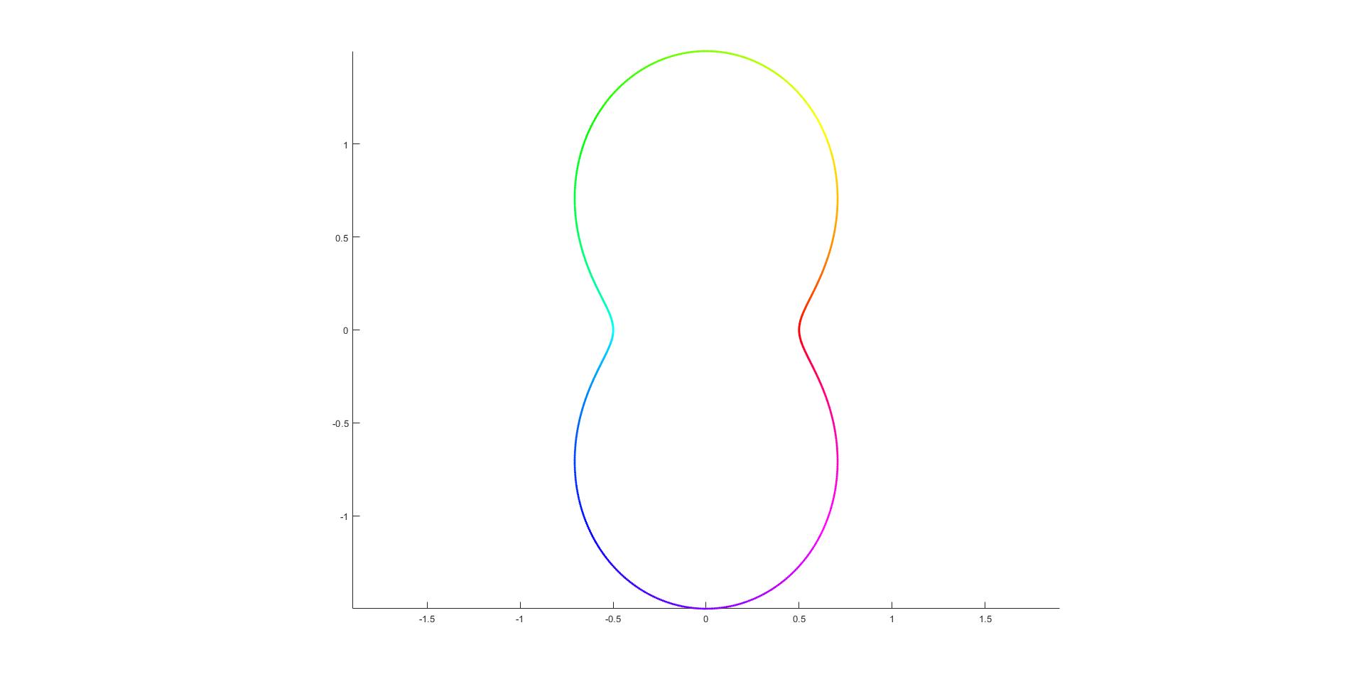
(a) Domain $\Omega_{1}$ with $\beta=0.5$

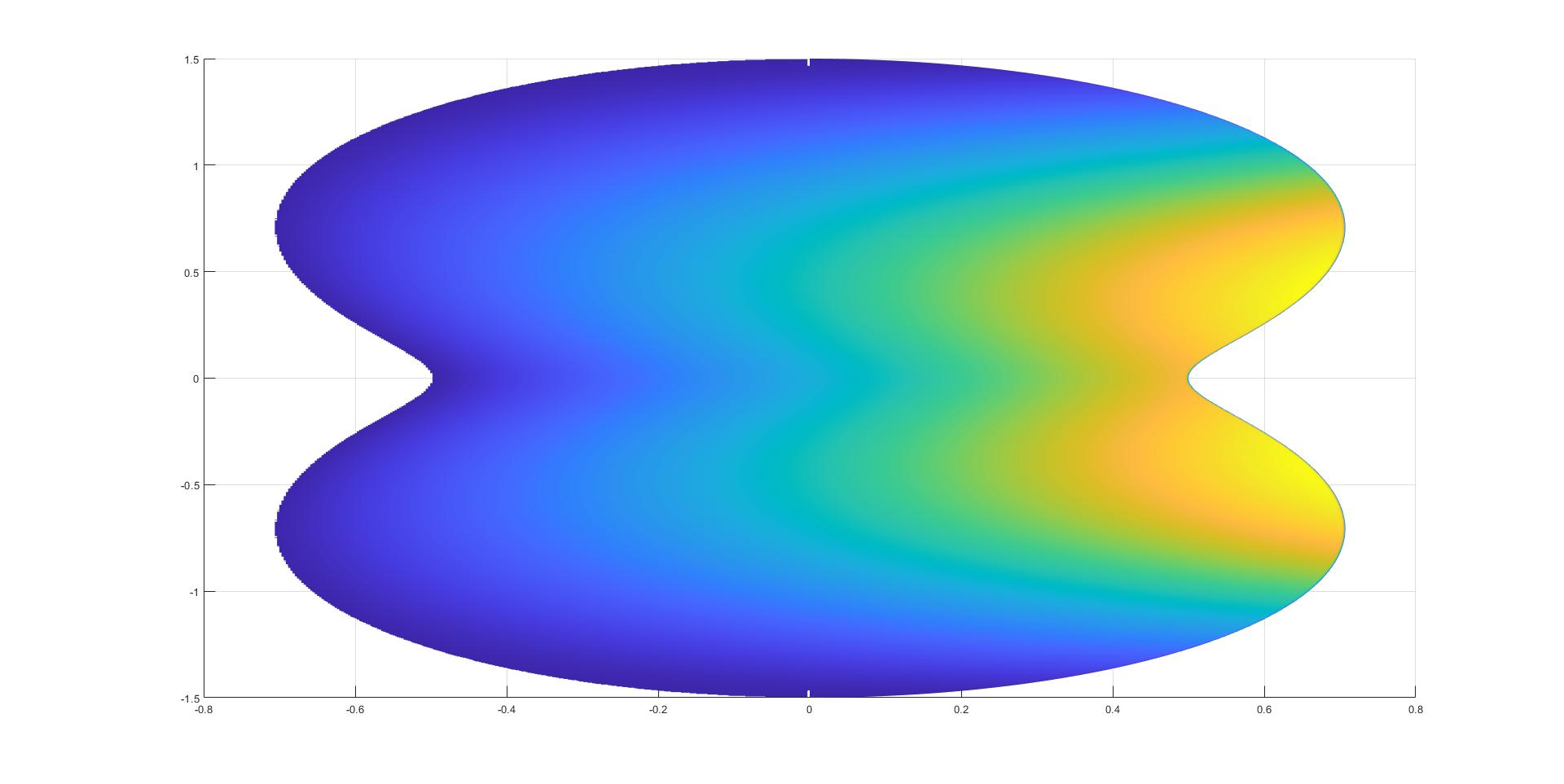
(b) Computed solution for $\varepsilon=10^{-3}$

Figure 1: Computed solution of problem (31) for $\varepsilon=10^{-3}$ on the domain $\Omega_{1}$ with $\beta=0.5$

In Table 1 we present orders for the following test problem:

$$-\varepsilon\triangle u+u_{x}+u=(1+\beta)^{2}-y^{2},\ (x,y)\in\Omega_{1},\quad u=0,\ (x,y)\in\partial\Omega_{1}$$ (31)

A sample computed solution is displayed in Figure 1.

$\varepsilon|N$	$N=8$	16	32	64	128	256	512
1.000000	0.5137	0.5011	1.4917	0.2148	1.7443	0.0500	1.3869
0.500000	0.1955	0.6965	1.3812	0.2949	1.7130	0.0752	1.3852
0.250000	-0.1489	0.8925	1.0994	0.5916	1.2696	0.5234	1.3834
0.125000	-0.1181	0.9350	1.0108	0.7912	1.0026	0.8120	1.3808
0.062500	0.1995	0.8365	0.3256	1.4904	0.7879	1.0620	1.2017
0.031250	0.4192	0.5178	-0.0990	1.5718	0.6644	1.0636	1.0025
0.015625	0.5074	0.5854	-0.1666	1.5261	0.9509	1.1332	1.0657
0.007813	0.5821	0.8212	0.0382	1.8144	1.2916	0.6715	1.3201
0.003906	0.6319	0.8092	0.7434	1.1094	1.2111	0.7548	1.2573
0.001953	0.6607	0.8019	0.9146	0.9390	1.0947	0.8686	1.1738
0.000977	0.6763	0.7984	0.9101	0.9444	1.0248	0.9377	1.0889
0.000488	0.6843	0.7968	0.9093	0.9455	0.9887	0.9737	1.0304
0.000244	0.6884	0.7961	0.9093	0.9455	0.9796	0.9558	1.0201
0.000122	0.6905	0.7958	0.9095	0.9453	0.9830	0.9489	0.9877
0.000061	0.6915	0.7956	0.9096	0.9452	0.9823	0.9643	0.9623
0.000031	0.6920	0.7955	0.9097	0.9452	0.9806	0.9818	0.9536
0.000015	0.6923	0.7955	0.9097	0.9451	0.9787	0.9837	0.9731
0.000008	0.6924	0.7955	0.9098	0.9451	0.9778	0.9846	0.9941
0.000004	0.6925	0.7955	0.9098	0.9451	0.9773	0.9851	0.9940
0.000002	0.6925	0.7954	0.9098	0.9451	0.9769	0.9855	0.9604
0.000001	0.6926	0.7954	0.9098	0.9451	0.9766	0.9780	0.9448
$\bar{p}^{N}$	0.6558	0.6238	-0.1517	1.5261	0.7629	1.0636	1.0025

Table 1: Computed double-mesh global orders of convergence $\bar{p}_{\varepsilon}^{N}$ for the corrected approximations $\bar{U}$ for problem (31) and $\beta=0.5$.

Remark 4.

In determing the double-mesh global orders of convergence, we note that we can underestimate the orders due to a potential overestimate of the maximum two mesh differences. This overestimate is caused by the fact that the interpolant $\bar{U}_{0}$ over the rectangular grid, will use mesh points lying within the strip $\bar{\Omega}_{S}$. This overspill is visible in Figure 2. An overestimate can occur when the maximum two mesh differences are located near the inner boundary of the strip.

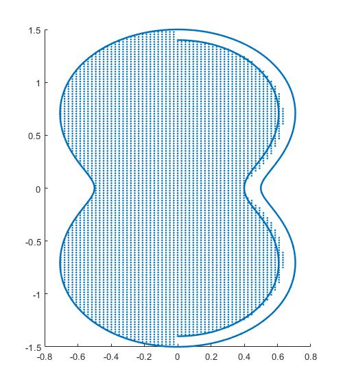
Figure 2: Example 1: Location of mesh points used in the calculation of $\bar{U}_{0}(x,y),\ (x,y)\in\Omega\setminus\Omega_{S}$, with $N=128$ on the rectangular grid

Example 2 The boundary is $\partial\Omega_{2}:=\{(\rho\sin t,\rho\cos t)\}$, with $\rho:=2.5*\pi^{2}+\beta-t^{2}\sin^{2}t$. In this case the orientation of the curve is clockwise as the parameter $t$ increases and the domain is not symmetrical. This domain does not have a smooth boundary at $t=0$, where there is a jump ($|[\kappa](0)|\approx 0.1246$) in the curvature. However, this point does not lie within the outflow boundary and hence it does not have any adverse effect on the rates of convergence. There are two external characteristic points at $(0,\pm M_{y}),M_{y}=2.5*\pi^{2}+\beta$. Also $M_{x}=2.25\pi^{2}+\beta$ and the upper bound in (24) is $R\approx<14.28$. In Table 2 we present global orders for the test problem, with $R=1$:

$$-\varepsilon\triangle u+u_{x}+u=\Bigl{(}(1-\frac{y^{2}}{M_{y}^{2}})(\frac{x}{M_{x}})\Bigr{)}^{4},\ (x,y)\in\Omega_{2},\ u=0,\ (x,y)\in\partial\Omega_{2}.$$ (32)

A sample computed solution is displayed in Figure 3.

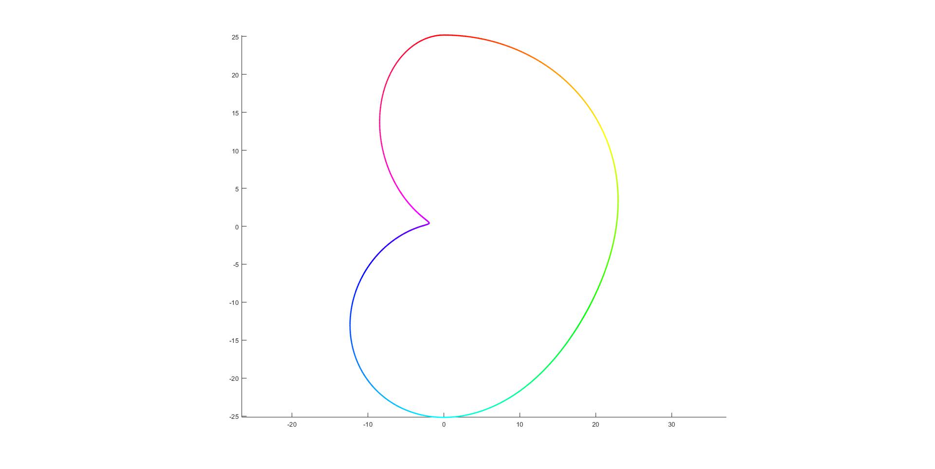
(a) Domain $\Omega_{2}$ with $\beta=0.5$

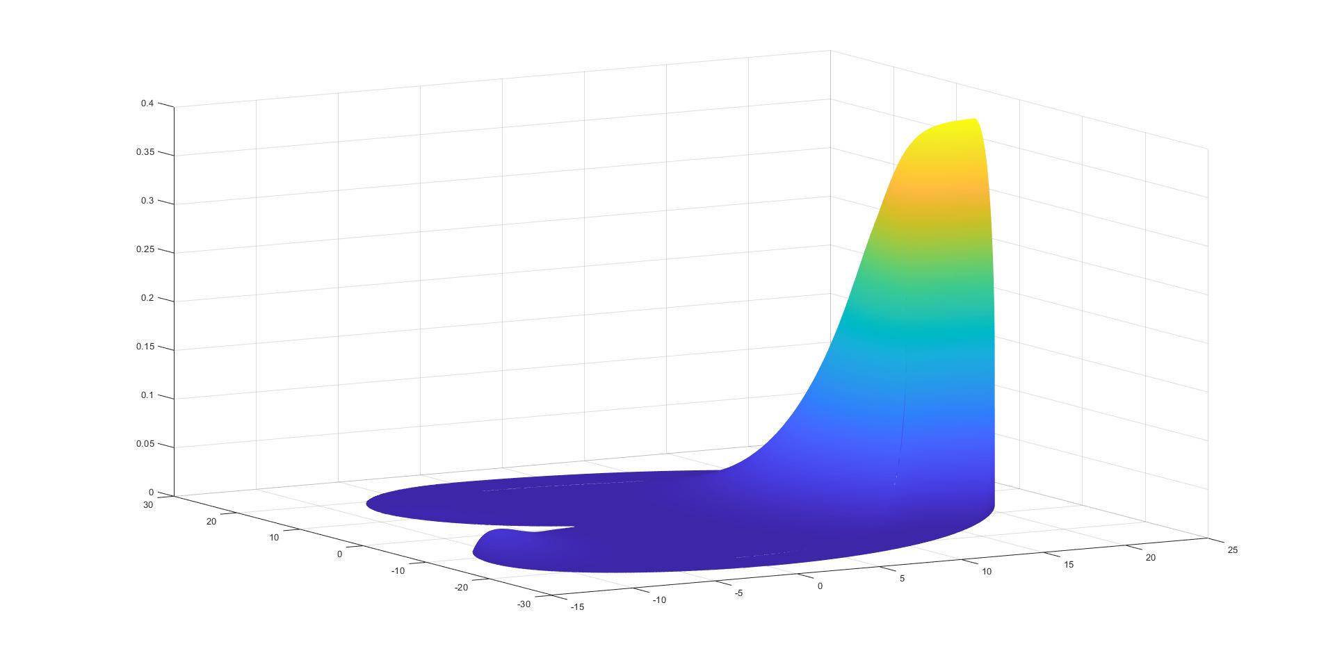
(b) Computed solution for $\varepsilon=2^{-10}$

Figure 3: Computed solution of problem (32) for $\varepsilon=2^{-10}$ on the domain $\Omega_{2}$ with $\beta=0.5$

$\varepsilon|N$	$N=8$	16	32	64	128	256	512
1.000000	1.1815	0.8659	1.2460	0.7149	2.1452	0.4748	2.0765
0.500000	1.5030	0.9087	0.7154	1.0345	1.1353	1.4214	1.2746
0.250000	1.6797	1.0045	0.6723	1.1996	1.7662	1.0373	0.9828
0.125000	1.6394	1.2235	1.4583	0.9942	0.9491	0.9721	0.9782
0.062500	1.6173	1.3528	1.2847	0.9799	0.9524	0.9745	0.9955
0.031250	1.6061	1.3424	0.9507	0.9831	0.9934	0.9969	0.9986
0.015625	1.6006	0.4432	0.9738	0.9372	0.9678	0.9833	0.9913
0.007813	1.5978	0.6144	0.6812	0.8724	0.7878	0.7226	0.7270
0.003906	1.5964	0.6192	0.6815	0.8722	0.7880	0.7225	0.8377
0.001953	1.5957	0.6216	0.6816	0.8721	0.7881	0.7224	0.8377
0.000977	1.5954	0.6228	0.6816	0.8720	0.7881	0.7224	0.8377
0.000488	1.5952	0.6234	0.6817	0.8720	0.7881	0.7224	0.8377
0.000244	1.5951	0.6237	0.6817	0.8720	0.7881	0.7224	0.8377
0.000122	1.5951	0.6238	0.6817	0.8720	0.7882	0.7224	0.8377
0.000061	1.5951	0.6239	0.6817	0.8720	0.7881	0.7224	0.8377
0.000031	1.5951	0.6239	0.6817	0.8720	0.7881	0.7224	0.8377
0.000015	1.5951	0.6239	0.6817	0.8720	0.7881	0.7224	0.8377
0.000008	1.5951	0.6240	0.6817	0.8720	0.7881	0.7224	0.8377
0.000004	1.5951	0.6240	0.6817	0.8720	0.7881	0.7224	0.8377
0.000002	1.5951	0.6240	0.6817	0.8720	0.7881	0.7224	0.8377
0.000001	1.5951	0.6240	0.6817	0.8720	0.7881	0.7224	0.8377
$\bar{p}^{N}$	1.5951	0.4599	0.8440	0.8724	0.7878	0.7226	0.7270

Table 2: Computed double-mesh global orders of convergence $\bar{p}_{\varepsilon}^{N}$ for the corrected approximations $\bar{U}$, using a strip of width $R=1$, for problem (32) and $\beta=0.5$.

Example 3 The boundary is $\partial\Omega_{3}:=\{(\phi(t),\psi(t))\}=\{(\rho\cos t,\rho\sin t)\}$, where $\rho:=\beta+\cos^{2}t$ and $0<\beta<2$. The inflow boundary is disjointed and corresponds to the intervals (in the $t$ variable)

$$(0,\theta)\cup(\pi/2,\pi-\theta)\cup(\pi+\theta,3\pi/2)\cup(2\pi-\theta,2\pi),\quad\theta=\arcsin\sqrt{\frac{1+\beta}{3}}.$$

The domain has four exterior characteristic points (where for $\beta=0.5,\kappa=3/(2\sqrt{2})$) at

$$(\pm P,\pm Q),\quad P:=\frac{2(1+\beta)}{3}\sqrt{\frac{2-\beta}{3}}\quad Q:=\frac{2(1+\beta)}{3}\sqrt{\frac{1+\beta}{3}}$$

and two interior characteristic points (where for $\beta=0.5,\kappa=2$) at $(0,\pm\beta)$. A test problem can be

$$-\varepsilon\triangle u+u_{x}+u=(1-\frac{y}{\beta})^{4}(1+\frac{y}{\beta})^{4}H(y-\beta)H(y+\beta),\ (x,y)\in\Omega_{3},\ u=0,\ (x,y)\in\partial\Omega_{3};$$ (33)

where $H(\cdot)$ is the Heaviside unit step function.

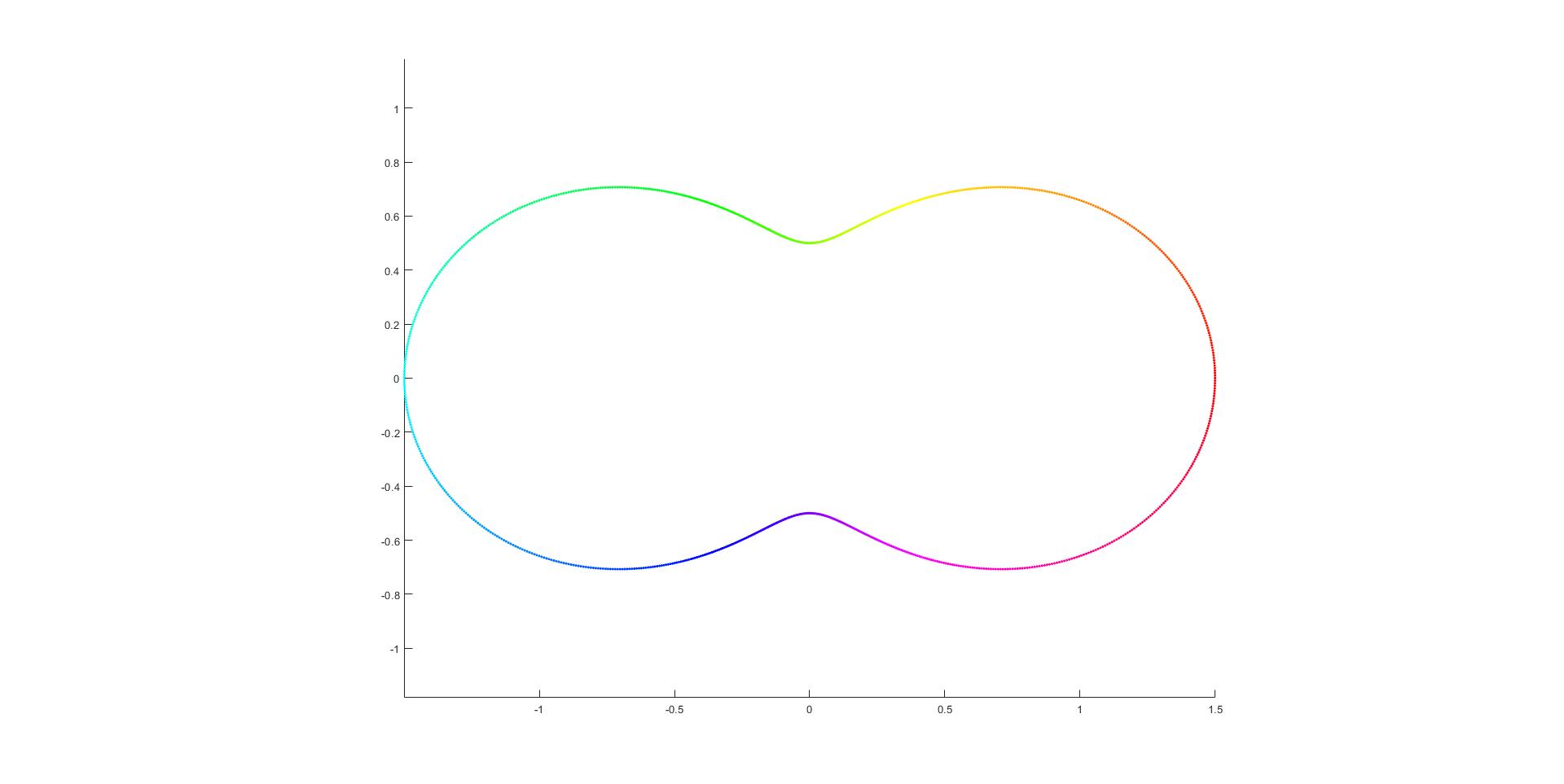
(a) Domain $\Omega_{3}$ with $\beta=0.5$

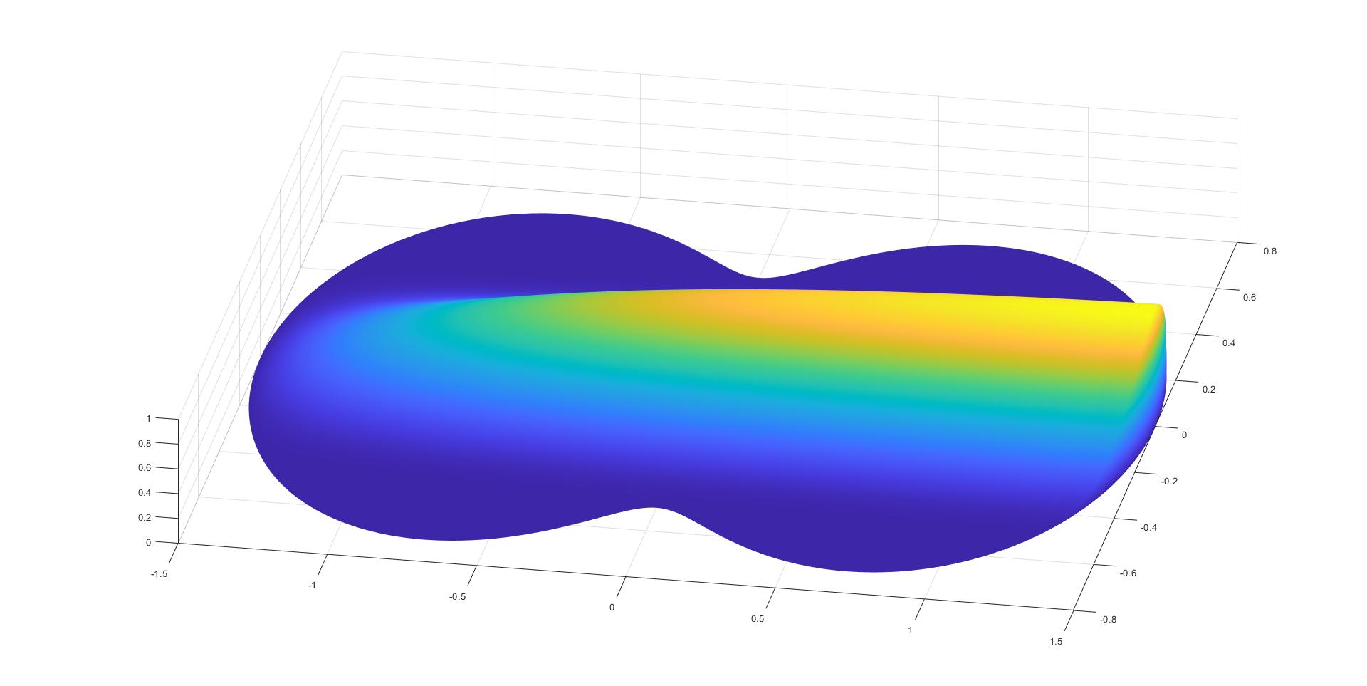
(b) Computed solution for $\varepsilon=2^{-10}$

Figure 4: Computed solution of problem (33) for $\varepsilon=2^{-10}$ on the domain $\Omega_{3}$ with $\beta=0.5$

$\varepsilon|N$	$N=8$	16	32	64	128	256	512
1.000000	1.0702	0.3644	0.8105	0.5711	0.6534	0.8372	0.6988
0.500000	1.3472	0.6217	0.7877	0.5623	0.6173	0.8308	0.8403
0.250000	1.1339	1.5496	0.7490	0.4977	0.5958	0.8188	0.8354
0.125000	0.8425	1.5538	1.0672	1.1292	0.5590	0.7984	0.8272
0.062500	0.5542	1.5041	0.8783	1.1497	1.0228	1.2867	0.9587
0.031250	0.3465	1.8518	0.8686	1.0378	1.0317	1.2056	1.0415
0.015625	0.2300	2.2651	1.2117	1.4030	1.3229	0.7461	0.8992
0.007813	0.1682	2.6703	1.5264	1.3204	0.8332	0.7949	0.9250
0.003906	0.1367	2.8922	1.6560	1.0698	0.7922	0.8311	0.9404
0.001953	0.1206	2.9286	1.6488	1.0898	0.7699	0.8540	0.9416
0.000977	0.1124	2.8983	1.6037	1.1256	0.8283	0.8676	0.9377
0.000488	0.1082	2.8689	1.4319	1.2229	0.9477	0.8704	0.9388
0.000244	0.1003	2.8576	1.3268	1.2763	1.0112	0.8838	0.9416
0.000122	0.0930	2.8554	1.2726	1.2552	1.0361	0.9471	0.9417
0.000061	0.0892	2.8547	1.2456	1.2200	1.0735	0.9525	0.9553
0.000031	0.0873	2.8544	1.2323	1.2028	1.0944	0.9378	0.9365
0.000015	0.0863	2.8542	1.2257	1.1943	1.1063	0.9313	0.9236
0.000008	0.0859	2.8542	1.2224	1.1902	1.1128	0.9290	0.9170
0.000004	0.0856	2.8542	1.2208	1.1882	1.1161	0.9283	0.9142
0.000002	0.0855	2.8542	1.2200	1.1871	1.1179	0.9282	0.9132
0.000001	0.0854	2.8541	1.2196	1.1866	1.1187	0.9281	0.9127
$\bar{p}^{N}$	0.0854	2.8541	1.0716	1.0378	1.0317	1.2056	1.0191

Table 3: Computed double-mesh global orders of convergence $\bar{p}_{\varepsilon}^{N}$ for the corrected approximations $\bar{U}$ for problem (33) and $\beta=0.5$.

Remark 5.

The data in test problem (33) has been chosen to satisfy Assumption 3, with $\delta=0.5$. The data in the test problems (31) and (32) do not staisfy the compatibility constraints in Assumption 3 for any choice of $\delta>0$. Nevertheless, for all three test problems we observe parameter-uniform convergence in each of the corresponding Tables of orders of convergence.

References

[1] M. Augustin, A. Caiazzo, A. Fiebach, J. Fuhrmann, V. John, A. Linke and R. Umla,
An assessment of discretizations for convection-dominated convection-diffusion equation, Comput. Methods Appl. Mech. Engrg., 200 (47-48), 2011, 3395–3409.
[2] G. Barrenechea, V. John, P. Knobloch and R. Rankin, A unified analysis of algebraic flux correction schemes for convection-diffusion equations, SeMA Journal. Boletin de la Sociedad Espanñola de Matemática Aplicada, 75 (4), 2018, 655–685.
[3] P.A. Farrell, A.F. Hegarty, J.J.H. Miller, E. O’Riordan and G.I. Shishkin, Robust computational techniques for boundary layers, CRC Press, 2000.
[4] B. García-Archilla, Shishkin mesh simulation: a new stabilization technique for convection-diffusion problems, Comput. Methods Appl. Mech. Engrg., 256, 2013, 1–16.
[5] D. Gilbarg and N. S. Trudinger, Elliptic partial differential equations of second order, Reprint of the third edition, Springer-Verlag, Berlin, 2001,
[6] N. Kopteva, Maximum norm error analysis of a 2D singularly perturbed semilinear reaction-diffusion problem, Math. Comp., 76 (258), (2007), 258, 631–646.
[7] A. M. Il’in, Matching of asymptotic expansions of solutions of boundary value problems, Mathematical Monographs, 102, American Mathematical Society, (1992).
[8] D. Frerichs and V. John, On reducing spurious oscillations in discontinuous Galerkin (DG) methods for steady-state convection-diffusion equations, J. Comput. Appl. Math., 2021, 113487, 20,
[9] O.A. Ladyzhenskaya and N.N. Ural’tseva, Linear and Quasilinear Elliptic Equations, Academic Press, New York and London, 1968.
[10] T. Linß and M. Stynes, Asymptotic analysis and Shishkin-type decomposition for an elliptic convection-diffusion problem, J. Math. Anal. and Applications, 261, 2001, 604–632.
[11] J.J.H. Miller, E. O’Riordan and G.I. Shishkin, Fitted Numerical Methods for Singular Perturbation Problems, World-Scientific, Singapore (Revised edition), 2012.
[12] H.-G. Roos, M. Stynes and L. Tobiska, Robust numerical methods for singularly perturbed differential equations, Springer Series in Computational Mathematics, 24, Second edition, Springer-Verlag, 2008.
[13] C. Schwab, M. Suri and C. Xenophontos, The finite element method for problems in mechanics with boundary layers,
Comput. Methods Appl. Mech. Engrg., 157 (3-4), 1998, 311–333.
[14] G.I. Shishkin and L.P. Shishkina, Discrete Approximation of Singular Perturbation Problems,
Chapman and Hall/CRC Press, 2008.
[15] C. Xenophontos and S. R. Fulton, Uniform approximation of singularly perturbed reaction-diffusion problems by the finite element method on a Shishkin mesh, Numer. Methods Partial Differential Equations, 19 (1), 2003, 89–111.