Low-frequency squeezing spectrum of a laser driven polar quantum emitter

Abstract

It was shown by a study of the incoherent part of the low-frequency resonance fluorescence spectrum of the polar quantum emitter driven by semiclassical external laser field and damped by non-squeezed vacuum reservoir that the emitted fluorescence field is squeezed to some degree nevertheless. As was also found, a higher degree of squeezing could, in principle, be achieved by damping the emitter by squeezed vacuum reservoir.

Keywords: polar emitter; fluorescence spectrum; squeezed vacuum; squeezed state; two-level atom; broken inversion symmetry; asymmetric quantum dot; polar molecule

1 Introduction

Squeezed states of electromagnetic (EM) field are of paramount importance to theoretical and experimental quantum physics because, besides other useful features, their statistically observable properties reveal true non-classical nature of light [1]. By now, these states have also found important technological applications in high precision measurements, spectroscopy, high resolution imaging techniques and optical communications. As a rule, experimental studies of squeezed states have been carried out with macroscopic sources of squeezed light despite that the possibility of squeezed light generation from a single two-level quantum emitter in free space was theoretically predicted long ago [2]. But only recently this prediction was experimentally proved to be the case for high-frequency resonance fluorescence in a semiconductor two-level quantum dot due its anomalously large transient dipole moment in comparison to those found in natural atoms an molecules [3]. It would be of theoretical as well as practical interest to find also a single-emitter source of squeezed low-frequency EM field. In the present study it is shown that a polar emitter represented by a simple two-level quantum system with broken inversion symmetry could play this role. Actually, violation of this symmetry is common in such natural systems as polar molecules as well as in artificially manufactured systems, like quantum dots. Due to this violation, these systems possess permanent dipole moments. The cause for the inversion symmetry violation is different for different systems. For example, in quantum dots the violation is induced by the asymmetry of the confining potential of the dot. Therefore, this asymmetry can be hugely augmented artificially in comparison to natural polar molecules, where its origin is due to the natural parity mixing of the molecular states [4]. However, in all cases this violation results in non-equal permanent diagonal dipole matrix elements of the ground and excited states. To our knowledge, the notion that a simple two-level quantum system driven by high-frequency classical EM field can emit EM field of much lower frequency if its dipole operator possesses permanent non-equal diagonal matrix elements, was revealed in [5] for the first time. This phenomenon was further studied thoroughly in [6, 7, 8] for the case of a two-level system driven by external EM field and damped by a dissipative thermal reservoir. The case of interaction with a broadband squeezed vacuum dissipative reservoir was studied earlier for weak driving EM field in [9, 10].

2 Model Hamiltonian

In this study we consider a two-level atom with ground state $|g\rangle$, excited state $|e\rangle$, transition frequency $\omega_{0}$ and the electric dipole moment $\hat{\bf d}$, driven by external classical monochromatic field ${\bf E}(t)={\bf E}\cos(\omega_{f}t)$ with an amplitude ${\bf E}$ and frequency $\omega_{f}$, and also coupled to a reservoir $B$ made of a plurality of modes of quantized electromagnetic field being in the squeezed vacuum state. It is assumed that the frequency Lamb shift due to interaction with the reservoir is already incorporated into the atomic transition frequency $\omega_{0}$. Thus, the model Hamiltonian reads

$$H=H_{S}(t)+\hbar\displaystyle\sum_{k}\omega_{k}b^{+}(\omega_{k})b(\omega_{k})+\displaystyle\sum_{k}\left(g(\omega_{k})S^{+}b(\omega_{k})+g^{*}(\omega_{k})b^{+}(\omega_{k})S^{-}\right).$$ (1)

Here $S^{+}=|e\rangle\langle g|$ and $S^{-}=|g\rangle\langle e|$ are the usual raising and lowering atomic operators and $S^{z}=\frac{1}{2}(|e\rangle\langle e|-|g\rangle\langle g|)$ is the atomic population inversion operator. The operators $b(\omega_{k})$ and $b^{+}(\omega_{k})$ are the annihilation and creation operators for the vacuum modes satisfying the commutation relations

$$[b(\omega),b^{+}(\omega^{\prime})]=\delta(\omega-\omega^{\prime}),\,\,[b(\omega),b(\omega^{\prime})]=0,\,\,[b^{+}(\omega),b^{+}(\omega^{\prime})]=0,$$ (2)

and the term

$$H_{S}(t)=\hbar\omega_{0}S^{z}+\frac{\hbar}{2}\Omega_{R}(S^{-}e^{i\omega_{f}t}+S^{+}e^{-i\omega_{f}t})+\frac{\hbar}{2}(e^{i\omega_{f}t}+e^{-i\omega_{f}t})\left[\delta_{a}S^{z}-\frac{\delta_{s}}{2}(|e\rangle\langle e|+|g\rangle\langle g|)\right]$$ (3)

contains an interaction between the driving field and the atom in the rotating wave approximation (RWA). Here $\Omega_{R}=-\bf Ed_{eg}/\hbar$ is the Rabi frequency being made real and positive by the appropriate choice of the phase factors of the states $|e\rangle$ and $|g\rangle$, and ${\bf d}_{eg}=e\langle e|\hat{\bf r}|g\rangle,\quad{\bf d}_{ge}=e\langle g|\hat{\bf r}|e\rangle,\quad{\bf d}_{ee}=e\langle e|\hat{\bf r}|e\rangle,\quad{\bf d}_{gg}=e\langle g|\hat{\bf r}|g\rangle$ are the atomic dipole moment operator matrix elements. As a rule, it is assumed that ${\bf d}_{ee}={\bf d}_{gg}=0$, because typical physical systems, like atoms and molecules, possess the inversion symmetry, and each of the states $|g\rangle$ and $|e\rangle$ is either symmetric or antisymmetric. Contrary to this view, we assume that the inversion symmetry of the system in question is violated, ${\bf d}_{ee}\neq{\bf d}_{gg}$, so that $\delta_{a}={\bf E}({\bf d}_{gg}-{\bf d}_{ee})/\hbar$ and $\delta_{s}={\bf E}({\bf d}_{gg}+{\bf d}_{ee})/\hbar$. The term proportional to $\delta_{s}$ does not influence the dynamics of the system and can be omitted, while the term proportional to the symmetry violation parameter $\delta_{a}$ is retained. The squeezed vacuum reservoir source is assumed to be broadband, and the squeezed vacuum field is characterized by the following correlation functions [11, 12]:

$$\langle b^{+}(\omega_{k})b(\omega_{k^{\prime}})\rangle_{svac}=N(r)\delta(\omega_{k}-\omega_{k^{\prime}}),\,\,\,\langle b(\omega_{k})\,b(\omega_{k^{\prime}})\rangle_{svac}=-M(r,\theta)\delta(\omega_{k}+\omega_{k^{\prime}}-2\omega_{s}),$$ (4)

$$\langle b(\omega_{k})b^{+}(\omega_{k^{\prime}})\rangle_{svac}\!=\!(N(r)+\!1)\delta(\omega_{k}\!-\!\omega_{k^{\prime}}),\langle b^{+}(\omega_{k}^{\prime})b^{+}(\omega_{k})\rangle_{svac}\!=\!-M^{*}(r,\theta)\delta(\omega_{k^{\prime}}+\omega_{k}\!-\!2\omega_{s}),$$ (5)

where $\omega_{s}$ is the carrier frequency of the squeezed field, $r$ is the degree of squeezing, $\theta$ is the phase of squeezing, $N(r)=\sinh^{2}(r)$ is related to the mean number of photons and $M(r,\theta)=\cosh(r)\sinh(r)\exp(i\theta)$ is characteristic of the squeezed vacuum field and describes the correlation between the two photons created in the down-conversion process.

3 Equations of Motion for Atomic Variables

In what follows, it is assumed that $\delta_{a}\ll\Omega_{R}$, so that the interaction of the driving field with the permanent dipole moment is much weaker than its interaction with the transitional dipole moment. It is also assumed that the driving field itself is weak. In the Markoff approximation the master equation for the atomic reduced density operator $\rho^{rf}_{S}(t)=e^{i\omega_{f}S^{z}t}\rho_{S}(t)e^{-i\omega_{f}S^{z}t}$ can be written in the frame rotating with the driving field frequency $\omega_{f}$ as

$$\frac{\partial\rho^{rf}_{S}(t)}{\partial t}=i\Gamma\delta[S^{z},\rho^{rf}_{S}(t)]-\frac{i}{2}\delta_{a}(e^{i\omega_{f}t}+e^{-i\omega_{f}t})[S^{z},\rho^{rf}_{S}(t)]+$$

$$+\frac{1}{2}\Gamma N(r)(2S^{+}\rho^{rf}_{S}(t)S^{-}-S^{-}S^{+}\rho^{rf}_{S}(t)-\rho^{rf}_{S}(t)S^{-}S^{+})+$$

$$+\frac{1}{2}\Gamma(N(r)+1)(2S^{-}\rho^{rf}_{S}(t)S^{+}-S^{+}S^{-}\rho^{rf}_{S}(t)-\rho^{rf}_{S}(t)S^{+}S^{-})-$$

$$-\Gamma M(r,\theta)S^{+}\rho^{rf}_{S}(t)S^{+}-\Gamma M^{*}(r,\theta)S^{-}\rho^{rf}_{S}(t)S^{-}-\frac{1}{2}i\Omega_{R}[S^{+}+S^{-},\rho^{rf}_{S}(t)],$$ (6)

under the assumption that the carrier frequency $\omega_{s}$ of the squeezed field coincides with the frequency $\omega_{f}$. Here $\Gamma$ is the radiative damping constant, $\delta=(\omega_{f}-\omega_{0})/\Gamma$. A closed set of equations follows from Eq.(6):

$$\!\frac{d\langle\tilde{S}^{-}(t)\rangle}{dt}\!=\!-\Gamma\left(\frac{1}{2}\!+\!N(r)\!-\!i\delta+i\frac{\delta_{a}}{2\Gamma}(e^{i\omega_{f}t}\!+e^{-i\omega_{f}t})\right)\!\langle\tilde{S}^{-}(t)\rangle+\Gamma M(r,\theta)\langle\tilde{S}^{+}(t)\rangle\!+\Omega_{R}\langle S^{z}(t)\rangle,$$ (7)

$$\!\frac{d\langle\tilde{S}^{+}(t)\rangle}{dt}\!=\!-\Gamma\left(\frac{1}{2}\!+\!N(r)\!+\!i\delta-i\frac{\delta_{a}}{2\Gamma}(e^{i\omega_{f}t}\!+\!e^{-i\omega_{f}t})\right)\!\langle\tilde{S}^{+}(t)\rangle+\Gamma\tilde{M}^{*}(r,\theta)\langle\tilde{S}^{-}(t)\rangle\!+\Omega_{R}\langle S^{z}(t)\rangle,$$ (8)

$$\frac{d\langle S^{z}(t)\rangle}{dt}=-\frac{1}{2}\Omega_{R}\left(\langle S^{-}(t)\rangle+\langle S^{+}(t)\rangle\right)-\Gamma(2N(r)+1)\langle S^{z}(t)\rangle-\Gamma/2,$$ (9)

where $\langle\tilde{S}^{\pm}(t)\rangle=\pm i\langle S^{\pm}(t)e^{\mp i\omega_{f}t}\rangle$ are slowly varying parts of the atomic operators. The system of equations (7-9) can be solved numerically by means of the technique employed earlier in [14], where the components of the vector $\vec{X}(t)=(\langle\tilde{S}^{-}(t)\rangle,\langle\tilde{S}^{+}(t)\rangle,\langle S^{z}(t)\rangle)$ are decomposed as $X_{i}(t)=\displaystyle\sum_{l=-\infty}^{+\infty}X_{i}^{(l)}(t)e^{il\omega_{f}t},\,i=1,2,3,$ and the slowly varying amplitudes $X_{i}^{(l)}(t)$ obey the system of equations

$$\frac{d}{dt}X_{1}^{(l)}(t)=-\Gamma\left(\frac{1}{2}+N(r)-i\delta+il\frac{\omega_{f}}{\Gamma}\right)X_{1}^{(l)}(t)-$$

$$-i\frac{\delta_{a}}{2}(X_{1}^{(l-1)}(t)+X_{1}^{(l+1)}(t))+\Gamma M(r,\theta)X_{2}^{(l)}(t)+\Omega_{R}X_{3}^{(l)}(t),$$ (10)

$$\frac{d}{dt}X_{2}^{(l)}(t)=-\Gamma\left(\frac{1}{2}+N(r)-i\delta+il\frac{\omega_{f}}{\Gamma}\right)X_{2}^{(l)}(t)+$$

$$+i\frac{\delta_{a}}{2}(X_{2}^{(l-1)}(t)+X_{2}^{(l+1)}(t))+\Gamma M^{*}(r,\theta)X_{1}^{(l)}(t)+\Omega_{R}X_{3}^{(l)}(t),$$ (11)

$$\frac{d}{dt}X_{3}^{(l)}(t)=-\frac{\Gamma}{2}\delta_{l,0}-(\Gamma(2N(r)+1)+il\omega_{f})X_{3}^{(l)}(t)-\frac{\Omega_{R}}{2}(X_{1}^{(l)}(t)+X_{2}^{(l)}(t)).$$ (12)

4 Low-frequency squeezing spectrum

The incoherent part of the fluorescence spectrum can be broken down into three contributions [15, 16]

$$F_{inc}(\omega)=F_{X}(\omega)+F_{Y}(\omega)+F_{as}(\omega),$$ (13)

$$F_{X}(\omega)=\frac{\Gamma}{2\pi}\mbox{Re}\displaystyle\int_{0}^{\infty}d\tau\lim_{t\to\infty}\left[\langle\tilde{S}^{+}(t)\tilde{S}^{-}(t+\tau)\rangle-\langle\tilde{S}^{+}(t)\rangle\tilde{\langle}S^{-}(t+\tau)\rangle\right.+$$

$$\left.+\langle\tilde{S}^{+}(t)\tilde{S}^{+}(t+\tau)\rangle-\langle\tilde{S}^{+}(t)\rangle\langle\tilde{S}^{+}(t+\tau)\rangle\right]\cos\Big{(}(\omega-\omega_{f})\tau\Big{)},$$ (14)

$$F_{Y}(\omega)=\frac{\Gamma}{2\pi}\mbox{Re}\displaystyle\int_{0}^{\infty}d\tau\lim_{t\to\infty}\left[\langle\tilde{S}^{+}(t)\tilde{S}^{-}(t+\tau)\rangle-\langle\tilde{S}^{+}(t)\rangle\langle\tilde{S}^{-}(t+\tau)\rangle\right.-$$

$$\left.-\langle\tilde{S}^{+}(t)\tilde{S}^{+}(t+\tau)\rangle+\langle\tilde{S}^{+}(t)\rangle\langle\tilde{S}^{+}(t+\tau)\rangle\right]\cos\Big{(}(\omega-\omega_{f})\tau\Big{)},$$ (15)

$$F_{as}(\omega)=-\frac{\Gamma}{\pi}\mbox{Im}\displaystyle\int_{0}^{\infty}d\tau\lim_{t\to\infty}\left[\langle\tilde{S}^{+}(t)\tilde{S}^{-}(t+\tau)\rangle-\langle\tilde{S}^{+}(t)\rangle\langle\tilde{S}^{-}(t+\tau)\rangle\right]\sin\Big{(}(\omega-\omega_{f})\tau\Big{)},$$ (16)

where $F_{Y}(\omega)$ and $F_{Y}(\omega)$ are in-phase and out-of-phase quadrature components of the noise spectrum, and $F_{as}(\omega)$ is the asymmetric contribution. Because of the so-called quantum regression hypothesis [12, 13], the fluctuation correlation functions $Y_{1}(t,t+\tau)=\langle\tilde{S}^{+}(t)\tilde{S}^{-}(t+\tau)\rangle-\langle\tilde{S}^{+}(t)\rangle\langle\tilde{S}^{-}(t+\tau)\rangle,$ $Y_{2}(t,t+\tau)=\langle\tilde{S}^{+}(t)\tilde{S}^{+}(t+\tau)\rangle-\langle\tilde{S}^{+}(t)\rangle\langle\tilde{S}^{+}(t+\tau)\rangle,$   $Y_{3}(t,t+\tau)=\langle\tilde{S}^{+}(t)\tilde{S}^{z}(t+\tau)\rangle-\langle\tilde{S}^{+}(t)\rangle\langle\tilde{S}^{z}(t+\tau)\rangle,$ satisfy virtually the same set of equations of motion (7-9) for the correspondent averages $\langle\tilde{S}^{-}(\tau)\rangle$, $\langle\tilde{S}^{+}(\tau)\rangle$ and $\langle\tilde{S}^{z}(\tau)\rangle$ with the only difference that the inhomogeneity $-\Gamma/2$ disappears due to the subtraction of the mean. These correlation functions can be decomposed as $Y_{i}(t,t+\tau)=\displaystyle\sum_{l=-\infty}^{+\infty}Y_{i}^{(l)}(t,\tau)e^{il\omega_{f}(t+\tau)}$, $i=1,2,3,$ so that

$$\frac{d}{d\tau}Y_{1}^{(l)}(t,\tau)=-\Gamma\left(\frac{1}{2}+N(r)-i\delta+il\frac{\omega_{f}}{\Gamma}\right)Y_{1}^{(l)}(t,\tau)-$$

$$-i\frac{\delta_{a}}{2}(Y_{1}^{(l-1)}(t,\tau)+Y_{1}^{(l+1)}(t,\tau))+\Gamma M(r,\theta)Y_{2}^{(l)}(t,\tau)+\Omega_{R}Y_{3}^{(l)}(t,\tau),$$ (17)

$$\frac{d}{d\tau}Y_{2}^{(l)}(t,\tau)=-\Gamma\left(\frac{1}{2}+N(r)-i\delta+il\frac{\omega_{f}}{\Gamma}\right)Y_{2}^{(l)}(t,\tau)+$$

$$+i\frac{\delta_{a}}{2}(Y_{2}^{(l-1)}(t,\tau)+Y_{2}^{(l+1)}(t,\tau))+\Gamma M^{*}(r,\theta)Y_{1}^{(l)}(t,\tau)+\Omega_{R}Y_{3}^{(l)}(t,\tau),$$ (18)

$$\frac{d}{d\tau}Y_{3}^{(l)}(t,\tau)=-(\Gamma(2N(r)+1)+il\omega_{f})Y_{3}^{(l)}(t,\tau)-\frac{\Omega_{R}}{2}(Y_{1}^{(l)}(t,\tau)+Y_{2}^{(l)}(t,\tau)),$$ (19)

and the Laplace transforms $\bar{Y}_{i}^{(l)}(t,z)=\displaystyle\int_{0}^{\infty}e^{-z\tau}Y_{i}^{(l)}(t,\tau)d\tau$ will satisfy the following set of equations:

$$z\bar{Y}_{1}^{(l)}(t,z)+\Gamma\left(\frac{1}{2}+N(r)-i\delta+il\frac{\omega_{f}}{\Gamma}\right)\bar{Y}_{1}^{(l)}(t,z)+$$

$$+i\frac{\delta_{a}}{2}\left(\bar{Y}_{1}^{(l-1)}(t,z)+\bar{Y}_{1}^{(l+1)}(t,z)\right)-\Gamma M(r,\theta)Y_{2}^{(l)}(t,z)-\Omega_{R}\bar{Y}_{3}^{(l)}(t,z)=$$

$$=\frac{1}{2}\delta_{l,0}+X_{3}^{(l)}(t)-\displaystyle\sum_{r=-\infty}^{\infty}X_{1}^{(l-r)}(t)X_{2}^{(r)}(t),$$ (20)

$$z\bar{Y}_{2}^{(l)}(t,z)+\Gamma\left(\frac{1}{2}+N(r)-i\delta+il\frac{\omega_{f}}{\Gamma}\right)\bar{Y}_{2}^{(l)}(t,z)-$$

$$-i\frac{\delta_{a}}{2}\left(\bar{Y}_{2}^{(l-1)}(t,z)+\bar{Y}_{2}^{(l+1)}(t,z)\right)-\Gamma M^{*}(r,\theta)Y_{1}^{(l)}(t,z)-\Omega_{R}\bar{Y}_{3}^{(l)}(t,z)=$$

$$=-\displaystyle\sum_{r=-\infty}^{\infty}X_{2}^{(l-r)}(t)X_{2}^{(r)}(t),$$ (21)

$$z\bar{Y}_{3}^{(l)}(t,z)+(\Gamma(2N(r)+1)+il\omega_{f})\bar{Y}_{3}^{(l)}(t,z)+\frac{\Omega_{R}}{2}(\bar{Y}_{1}^{(l)}(t,z)+\bar{Y}_{2}^{(l)}(t,z))=$$

$$=-\displaystyle\sum_{r=-\infty}^{\infty}\left(\frac{1}{2}\delta_{r,0}+X_{3}^{(r)}(t)\right)X_{2}^{(l-r)}(t).$$ (22)

In the steady state limit $(t\to\infty)$ only the zero-order components $\bar{Y}_{1,2}^{(0)}(t,z)$ contributes to $F_{inc}(\omega)$. Therefore,

$$F_{X}(\omega)=\frac{\Gamma}{4\pi}\mbox{Re}\lim_{t\to\infty}\left[[\bar{Y}_{1}^{(0)}(t,z)+\bar{Y}_{2}^{(0)}(t,z)]\Big{|}_{z=-i(\omega-\omega_{f})}+[\bar{Y}_{1}^{(0)}(t,z)+\bar{Y}_{2}^{(0)}(t,z)]\Big{|}_{z=i(\omega-\omega_{f})}\right],$$ (23)

$$F_{Y}(\omega)=\frac{\Gamma}{4\pi}\mbox{Re}\lim_{t\to\infty}\left[[\bar{Y}_{1}^{(0)}(t,z)-\bar{Y}_{2}^{(0)}(t,z)]\Big{|}_{z=-i(\omega-\omega_{f})}+[\bar{Y}_{1}^{(0)}(t,z)-\bar{Y}_{2}^{(0)}(t,z)]\Big{|}_{z=i(\omega-\omega_{f})}\right],$$ (24)

$$F_{as}(\omega)=\frac{\Gamma}{2\pi}\mbox{Re}\lim_{t\to\infty}\left[\bar{Y}_{1}^{(0)}(t,z)\Big{|}_{z=-i(\omega-\omega_{f})}-\bar{Y}_{1}^{(0)}(t,z)\Big{|}_{z=i(\omega-\omega_{f})}\right].$$ (25)

5 Numerical Results

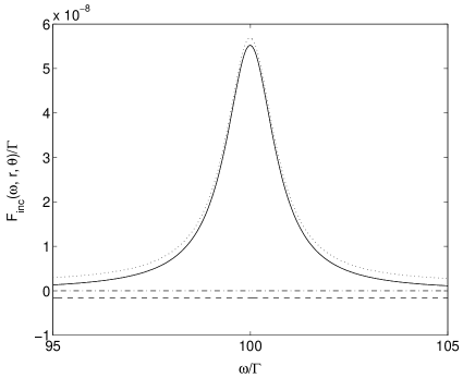
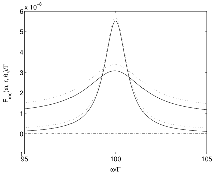
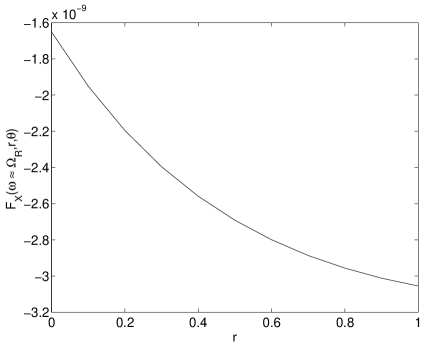
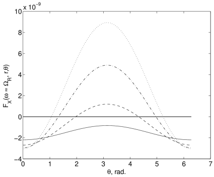
In this research, the case of the driving field frequency $\omega_{f}$ and the carrier frequency of the squeezed field $\omega_{s}$ being simultaneously in resonance with the atomic transition frequency $\omega_{0}$ was studied. Equations (10)-(12) and (20)-(22) were solved numerically, as usual [14], in the steady state limit $(t\to\infty)$ by truncation of the number of the harmonic amplitudes $X_{i}^{(l)}(t)$ and $\bar{Y}_{i}^{(l)}(t,z)$ taken into account. As was shown before [6] for a driven two-level system with broken symmetry interacting with non-squeezed vacuum reservoir, a low-frequency radiation peak centered nearly exactly at the frequency $\omega=\Omega_{R}$ appears in the fluorescence spectrum, see Fig.2. It is seen that the in-phase quadrature spectral component $F_{X}(\omega)$ is nearly uniformly negative, which means that the fluorescent field is squeezed (cf. [2, 17, 18, 19]) even without squeezing of the vacuum reservoir field. The increase in the vacuum squeezing degree $r$ results in the spectral amplitude decrease and the broadening of the radiation peak at $\omega=\Omega_{R}$, see Fig.2, while the component $F_{X}(\omega)$ steadily decreases, see Fig.4. The degree of the fluorescent field squeezing is strongly affected by the squeezing phase $\theta$ of the vacuum field, see Fig.4. For large enough $r$, there is a domain of $\theta$ values for which this squeezing totally disappears.

Figure 1: Fluorescence spectrum $F_{inc}$ and its components $F_{X}--$, $F_{Y}\cdot\cdot$, $F_{A}-\cdot-$.
$\Gamma=1,\,r=0,\theta=0,\,\omega_{f}=\omega_{s}=\omega_{0}=5000,\Omega_{R}=100,\delta_{a}=10$.

Figure 2: Fluorescence spectrum $F_{inc}$ and its components $F_{X}--$, $F_{Y}\cdot\cdot$, $F_{A}-\cdot-$.
$\Gamma=1,\,r=0,\,r=1,\,\theta=0,\,\omega_{f}=\omega_{s}=\omega_{0}=5000,\Omega_{R}=100,\delta_{a}=10$.

Figure 3: Fluorescence spectrum component $F_{X}$ at $\omega=\Omega_{R}$ for various values of $r$.
$\Gamma=1,\,\theta=0,\,\omega_{f}\!=\!\omega_{s}\!=\!\omega_{0}\!=\!5000,\Omega_{R}\!=\!100,\delta_{a}\!=\!10$.

Figure 4: Fluorescence spectrum component $F_{X}$ at $\omega=\Omega_{R}$ for various values of $r=0.2-,0.5--,0.8-\cdot-,1.0\cdot\cdot$ and $\theta$. $\Gamma=1,\,\omega_{f}\!=\!\omega_{s}\!=\!\omega_{0}\!=\!5000,\Omega_{R}\!=\!100,\delta_{a}\!=\!10$.

6 Conclusion

In conclusion, the effect of the broadband squeezed vacuum dissipative damping reservoir on the squeezing properties of the low-frequency fluorescence field emitted by a quantum two-level polar system with broken inversion symmetry driven by external high-frequency classical EM (laser) field was studied. As was found, the squeezing in the low-frequency fluorescent field already exists even without squeezing in the vacuum field. It was also shown that the presence of squeezing in the vacuum field can increase the degree of squeezing in the fluorescent field for appropriate values of the vacuum squeezing phase. At the same time, it is possible to alternate the amplitude and the spectral width of the low-frequency fluorescence spectral peak by changing the parameters of the squeezed vacuum, such as the squeezing degree $r$ and squeezing phase $\theta$.

References

• [1] Loudon R. and Knight P.L. 1987 J. Mod. Opt. 34 709-759
• [2] Walls D.F. and Zoller P. 1981 Phys. Rev. Lett. 47 no.10 709
• [3] Schulte C., Hansom J., Jones A., Matthiesen C., Le Gall C. and AtatΓΌre M. 2015 Nature 525 222-225
• [4] Kovarskii V.A. 1999 Phys. Usp. 42 797
• [5] Kibis O.V., Slepyan G.Ya., Maksimenko S.A. and Hoffmann A. 2009 Phys. Rev. Lett. 102 023601
• [6] Soldatov A.V. 2016 Mod. Phys. Lett. B 30 no.27 1650331
• [7] Soldatov A.V. 2017 Mod. Phys. Lett. B 34 no.4 1750027
• [8] Bogolyubov N.N.(Jr.) and Soldatov A.V. 2018 Mosc. Univ. Phys. Bull. 73 no.2 154-61
• [9] Bogolyubov N.N.(Jr.) and Soldatov A.V. 2020 Phys. Part. Nucl. 51:4 762
• [10] Bogolyubov N.N.(Jr.) and Soldatov A.V. 2020 Journ. of Phys.: Conf. Ser. 1560 12001
• [11] Gardiner C.W. 1986 Phys. Rev. Lett. 56 1917
• [12] Puri R.R. 2001 Mathematical Methods of Quantum Optics (Springer Series in Optical Sciences vol. 79) ( Berlin Heidelberg: Springer-Verlag)
• [13] Carmichael H. 1993 An Open Systems Approach to Quantum Optics (Lecture Notes in Physics vol. 18) (Berlin: Springer-Verlag)
• [14] Ficek Z., Seke J., Soldatov A.V. and Adam G. 2001 Phys. Rev. A 64 no.1 013813
• [15] Swain S. and Zhou P. 1996 Opt. Commun. 123 310
• [16] Carmichael H.J. 1987 J. Opt. Soc. Am. B4 1588
• [17] Collett M.J., Walls D.F. and Zoller P. 1984 Opt. Commun. 52 145
• [18] Ou Z.Y., Hong C.K. and Mandel L. 1987 J. Opt. Soc. Am. B 4 no.10 1574
• [19] Tana$\acute{s}$ R., Ficek Z., Messikh A. and El-Shahat T. 1998 J. Mod. Opt. 45 No. 9 1859-1883