Effects of weak magnetic field and finite chemical potential on the transport of charge and heat in hot QCD matter

Abstract

We have studied the effects of weak magnetic field and finite chemical potential on the transport of charge and heat in hot QCD matter by estimating their respective response functions, viz. the electrical conductivity ($\sigma_{\rm el}$), the Hall conductivity ($\sigma_{\rm H}$), the thermal conductivity ($\kappa_{0}$) and the Hall-type thermal conductivity ($\kappa_{1}$). The expressions of charge and heat transport coefficients are obtained by solving the relativistic Boltzmann transport equation in the relaxation time approximation at weak magnetic field and finite chemical potential. The interactions among partons are incorporated through their thermal masses. We have observed that $\sigma_{\rm el}$ and $\kappa_{0}$ decrease and $\sigma_{\rm H}$ and $\kappa_{1}$ increase with the magnetic field in the weak magnetic field regime. On the other hand, the presence of a finite chemical potential increases these transport coefficients. The effects of weak magnetic field and finite chemical potential on aforesaid transport coefficients are found to be more conspicuous at low temperatures, whereas at high temperatures, they have only a mild dependence on magnetic field and chemical potential. We have found that the presence of finite chemical potential further extends the lifetime of the magnetic field. Furthermore, we have explored the effects of weak magnetic field and finite chemical potential on the Knudsen number, the elliptic flow coefficient and the Wiedemann-Franz law.

1 Introduction

High temperatures and/or high densities create most favorable conditions for the transition of the normal nuclear matter to a deconfined state of quarks and gluons, known as quark-gluon plasma (QGP). Such conditions are realised in collisions of ultrarelativistic heavy ions at Relativistic Heavy Ion Collider (RHIC) at BNL and Large Hadron Collider (LHC) at CERN. In noncentral collisions, strong magnetic fields are produced in a direction perpendicular to the collision plane whose initial strength could be expressed in terms of the pion mass scale as $eB=m_{\pi}^{2}$ ($\simeq 10^{18}$ Gauss) at RHIC and $eB=15$ $m_{\pi}^{2}$ at LHC [1, 2] energies. Some of the phenomenological consequences of the strong magnetic fields are the chiral magnetic effect [3, 4], the axial magnetic effect [5, 6], the nonlinear electromagnetic current [7, 8], the axial Hall current [9], the chiral vortical effect [10] etc. Whether the magnetic field created leaves any observable effects in heavy ion collisions depends on the thermalization of light quarks in QGP which induces a large electrical conductivity. As a result, an electric current would be induced by virtue of Lenz’s law which might significantly elongate the lifetime of the magnetic field [11, 12, 13]. Therefore, it is pertinent to investigate the effects of magnetic field on the partonic medium. The observable effects of strong magnetic fields on various properties of hot medium of quarks and gluons have attracted much theoretical attention, e.g. the thermodynamic and magnetic properties [14, 15, 16, 17], the photon and dilepton productions from QGP [18, 19, 20, 21], the heavy quark diffusion [22], the magnetohydrodynamics [23, 24] etc.

The study of various transport coefficients is important as they provide information about the formation and evolution of the hot QCD matter. Two of such transport coefficients are the electrical conductivity ($\sigma_{\rm el}$) and the thermal conductivity ($\kappa$) which describe the charge transport and the heat transport in the medium, respectively. Besides the shear and bulk viscosities, the electrical and thermal conductivities are also vital for the hydrodynamic evolution of the strongly interacting matter at nonzero baryon densities [25, 26]. These conductivities can be determined by using various approaches, viz., the relativistic Boltzmann transport equation [27, 28, 29, 30], the correlator technique using Green-Kubo formula [31, 32, 33], the Chapman-Enskog approximation [34, 35], the lattice simulation [36, 37, 38] etc. In the presence of magnetic field, the transport coefficients no longer remain isotropic and they acquire multicomponent structures [39, 40, 41, 44, 45, 42, 43, 46, 47, 48, 49, 50, 51]. There exist three components for charge transport as well as for heat transport. However, under specific conditions, where electric and magnetic fields are perpendicular to each other and in weak magnetic field limit, some components vanish [33, 44, 48]. In the presence of a magnetic field, quarks experience a Lorentz force and it results in an induced electric current along a direction transverse to both electric and magnetic fields, and the conductivity associated with this current is known as Hall conductivity [33]. For pair plasma having equal numbers of charged particles and antiparticles, the net Hall current vanishes [52, 53]. At zero chemical potential, quark-gluon plasma is analogous to the case of pair plasma. In this case, there will be no Hall effect due to the exact cancellation of Hall current contributions from particles and their antiparticles. However, at finite chemical potential, the asymmetry between the numbers of quarks and antiquarks develops a suitable condition for the production of finite Hall current. In the weak magnetic field regime, one can assume that the phase space and the single particle energies are not affected by the magnetic field through Landau quantization as in ref. [33] and the main contribution of the effect of magnetic field on the transport coefficients comes through the cyclotron frequency.

The effects of magnetic field on the abovementioned transport coefficients had been studied previously using different models and approximations at finite magnetic field. For example, in ref. [54], the effect of magnetic field on the conductivities had been studied using the quenched SU(2) lattice gauge theory. Authors in references [44, 45] had estimated the conductivities using the relativistic Boltzmann transport equation in the relaxation time approximation, but for a hot and dense hadronic matter. In ref. [31], authors had exploited the Kubo formalism with the dilute instanton-liquid model to study the electrical conductivity in an external magnetic field. In ref. [55], the real time formalism with the diagrammatic method had been exploited to study the electrical conductivity in strong magnetic fields, whereas ref. [33] had employed the Kubo formalism and ref. [56] had used the quasiparticle model to explore the conductivities. Authors in ref. [57] had investigated the effect of magnetic field on the conductivities using the Landau level resummation via kinetic equations. In ref. [13], authors had studied the effects of the strong magnetic field-induced and asymptotic expansion-induced anisotropies on conductivities for a hot QCD matter using the kinetic theory approach, while in ref. [58], the collective effects of the strong magnetic field and density on conductivities had been explored. The effective fugacity approach had been implemented in references [59, 60] to investigate the effect of magnetic field on conductivities. In the present work, (i) we have studied both charge and heat transport coefficients for a QGP/hot QCD matter in the presence of both weak magnetic field and finite chemical potential. In this study, we have used the weak magnetic field limit, where the energy scale associated with the temperature of the QCD medium is larger than the energy scale related to the magnetic field, i.e. $T^{2}\gg eB$. So, we have used the ansatz method in the weak magnetic field limit to calculate the conductivities in section 2. (ii) We have extended our study to know the collective effects of weak magnetic field and density on some applications of conductivities, such as the Knudsen number, the elliptic flow and the Lorenz number in the Wiedemann-Franz law. (iii) We have used the thermal masses of particles. The particles acquire thermally generated masses due to their interactions with the thermal medium.

In studying the charge and heat transport coefficients for the hot and dense QCD matter, the kinetic theory approach within the relaxation time approximation has been used. Charge and heat transport coefficients are determined by solving the relativistic Boltzmann transport equation in weak magnetic field regime. The impact of weak magnetic field on the properties of QCD medium is expected to be significantly different from that of the strong magnetic field case. We also observe how the presence of finite chemical potential affects the lifetime of magnetic field. The use of thermal masses is relevant, because the medium formed in heavy ion collision behaves like a strongly coupled system and thus one cannot fully rely on the perturbative method and the interactions are contained only in the thermal masses of particles. Thermal masses have been calculated previously by different groups for different scenarios, viz., the Nambu-Jona-Lasinio (NJL) and Polyakov NJL based quasiparticle models [61, 62, 63], quasiparticle model with Gribov-Zwanziger quantization [64, 65], quasiparticle model in a strong magnetic field [66, 67], thermodynamically consistent quasiparticle model [68, 69, 70, 71] etc.

Due to the finite electrical conductivity in heavy ion collisions, electric current is produced, which is essential for the strength of chiral magnetic effect [3]. In addition, the strength of the charge asymmetric flow in mass asymmetric collisions depends on electrical conductivity [72]. The difference between energy flow and enthalpy flow in a thermal medium generates heat flow, which is associated with the thermal conductivity. In heavy ion collisions, thermal conductivity plays an important role in controlling the strength of hydrodynamic fluctuations [73]. Thus, any modification in the charge and heat transport coefficients might leave some noticeable impacts on the observables at heavy ion collisions. Some of their applications in the similar environment, such as the validity of the local equilibrium through the Knudsen number ($\Omega$), the elliptic flow ($v_{2}$) and the interplay between electrical and thermal conductivities through the Lorenz number ($L$) in the Wiedemann-Franz law have also been explored.

The rest of this paper is organized as follows. Section 2 is devoted to the study of charge and heat transport properties of hot and dense QCD matter in the presence of a weak magnetic field by using the kinetic theory approach. The effect of chemical potential on the lifetime of magnetic field in an electrically conducting medium is discussed in section 3. The results on aforesaid transport properties are discussed in section 4. Section 5 explores the applications of the obtained transport coefficients to estimate the Knudsen number, the elliptic flow coefficient and to study the relation between charge and heat transports through the Wiedemann-Franz law. The work is summarised in section 6.

2 Charge and heat transport properties of hot and dense QCD medium in a weak magnetic field

In this section, the charge and heat transport properties are studied in kinetic theory approach by calculating corresponding transport coefficients. In particular, subsection 2.1 contains the calculation of components of charge transport and subsection 2.2 is devoted to the calculation of components of heat transport for the hot and dense QCD medium in the presence of a weak magnetic field.

To calculate the transport coefficients, we solve the relativistic Boltzmann transport equation by following the relaxation time approximation. In general, the Boltzmann transport equation is a complicated nonlinear integro-differential equation for particle distribution function $f(p)$, which gets linearized through the relaxation time approximation, and this can be understood as follows. Frequent collisions among particles help the system in bringing back to the equilibrium state and in this process the Boltzmann transport equation expresses the evolution of the particle distribution function as

$$\frac{df(\mathbf{p})}{dt}=\left(\frac{df(\mathbf{p})}{dt}\right)_{\rm coll}.$$ (1)

In a time interval $dt$, the probability of occupation of a parton with momentum $\mathbf{p}$ after it gets scattered into the volume element $d\mathbf{p^{\prime}}$ about $\mathbf{p^{\prime}}$ is written as $\Gamma_{\mathbf{p},\mathbf{p^{\prime}}}dtd\mathbf{p^{\prime}}/(2\pi)^{3}$, where $\Gamma_{\mathbf{p},\mathbf{p^{\prime}}}$ is the matrix element discerning the scattering of partons in and out of the aforesaid volume element. Denoting $\tau(\mathbf{p})$ as the relaxation time, the probability per unit time that a parton at $\mathbf{p}$ gets scattered into $\mathbf{p^{\prime}}$ is given by

$$\frac{1}{\tau(\mathbf{p})}=\int\frac{d\mathbf{p^{\prime}}}{(2\pi)^{3}}\Gamma_{\mathbf{p},\mathbf{p^{\prime}}}\left(1-f(\mathbf{p^{\prime}})\right).$$ (2)

The number of partons per unit volume in $d\mathbf{p}$ about $\mathbf{p}$ experiencing a collision within a time interval $dt$ is $\frac{dt}{\tau(\mathbf{p})}{f(\mathbf{p})d\mathbf{p}}/{(2\pi)^{3}}$, which can also be represented as   $-\left(\frac{df(\mathbf{p})}{dt}\right)_{\rm out}{d\mathbf{p}dt}/{(2\pi)^{3}}$. Thus, the number of partons going out of the aforesaid volume element after suffering collisions is obtained as

$$\left(\frac{df(\mathbf{p})}{dt}\right)_{\rm out}=-\frac{f(\mathbf{p})}{\tau(\mathbf{p})}.$$ (3)

After substituting the value of $1/\tau(\mathbf{p})$ (2) in eq. (3), one gets

$$\left(\frac{df(\mathbf{p})}{dt}\right)_{\rm out}=-f(\mathbf{p})\int\frac{d\mathbf{p^{\prime}}}{(2\pi)^{3}}\Gamma_{\mathbf{p},\mathbf{p^{\prime}}}\left(1-f(\mathbf{p^{\prime}})\right).$$ (4)

In the similar way, the number of partons scattered into the volume element $d\mathbf{p}$ about $\mathbf{p}$ is expressed as

$$\left(\frac{df(\mathbf{p})}{dt}\right)_{\rm in}=\left(1-f(\mathbf{p})\right)\int\frac{d\mathbf{p^{\prime}}}{(2\pi)^{3}}\Gamma_{\mathbf{p^{\prime}},\mathbf{p}}f(\mathbf{p^{\prime}}).$$ (5)

The evolution of the distribution function or the collision term is mainly contributed by the partons scattering in and out of the volume element due to collisions. Thus, we have

$$\left(\frac{df(\mathbf{p})}{dt}\right)_{\rm coll} = \left(\frac{df(\mathbf{p})}{dt}\right)_{\rm out}+\left(\frac{df(\mathbf{p})}{dt}\right)_{\rm in}$$ (6)

$$= -\int\frac{d\mathbf{p^{\prime}}}{(2\pi)^{3}}\left[\Gamma_{\mathbf{p},\mathbf{p^{\prime}}}f(\mathbf{p})\left(1-f(\mathbf{p^{\prime}})\right)-\Gamma_{\mathbf{p^{\prime}},\mathbf{p}}f(\mathbf{p^{\prime}})\left(1-f(\mathbf{p})\right)\right],$$

which is a nonlinear integro-differential Boltzmann transport equation. To find a solution of the Boltzmann transport equation, some simplifying approximations are needed. One of the frequently used simplifications for the collision term is known as the relaxation time approximation. This method is useful in linearizing the Boltzmann transport equation through the following assumptions: (i) The distribution function gets infinitesimally deviated from its equilibrium, so that within a phenomenological timescale (the relaxation time) $\tau$, the system returns back to the equilibrium state. (ii) The probability per unit time for a collision, i.e., ${1}/{\tau(\mathbf{p})}$ no longer depends on the parton distribution function. (iii) The number of partons scattering into the phase space volume element, involve the equilibrium distribution function, whereas the number of partons which move out of the concerned phase space volume element after suffering collisions, involve the nonequilibrium distribution function. So, the collision term, i.e. the rate at which the distribution function changes due to collisions becomes

$$\left(\frac{df(\mathbf{p})}{dt}\right)_{\rm coll}=-\frac{\left(f(p)-f_{0}(p)\right)}{\tau}.$$ (7)

Thus, the Boltzmann transport equation takes the linearized form via the relaxation time approximation as

$$\frac{df(p)}{dt}=-\frac{\left(f(p)-f_{0}(p)\right)}{\tau}.$$ (8)

In the present work, we have considered the linearized Boltzmann transport equation in the relaxation time approximation method.

It is known that the relaxation time approximation defies the local particle number conservation in the medium, because the charge is not conserved instantaneously but only on the average over a cycle. However, the validity of the conservation laws can be guaranteed by imposing a condition that the relaxation time has no momentum dependence and this can be perceived as follows. In general, the Boltzmann transport equation for a single particle distribution function $f(x,p)$ is written as

$$p^{\mu}\partial_{\mu}f=\mathcal{C}[f]=\hat{L}\phi,$$ (9)

where $\hat{L}$ is the linearized collision operator, $f_{0}\phi=f-f_{0}=\delta f$ and $f_{0}$ denotes the equilibrium distribution function. The $\hat{L}$ has only the nonpositive eigenvalues, whose absolute values elucidate the reciprocal of the relaxation times of nonequilibrium perturbations and the eigenfunctions with zero eigenvalues are conserved in collisions, such as the particle number, energy and momentum [74, 75]. In the relaxation time approximation, eq. (9) changes to take the following form,

$$p^{\mu}\partial_{\mu}f=-\frac{\omega}{\tau}\delta f,$$ (10)

where $\omega=p_{0}$ is the energy of parton. In order to satisfy the fundamental conservation equations, the zeroth and the first moments of the collision integral must vanish, i.e. $\int dP~{}\mathcal{C}[f]=0$ and $\int dP~{}p^{\mu}\mathcal{C}[f]=0$, which follow from the particle number conservation and energy-momentum conservation, respectively. Thus, to check the conservation of the particle number, one needs to multiply both sides of eq. (10) with 1 and then integrate in momentum, i.e.,

$$\int dPp^{\mu}\partial_{\mu}f=-\int dP\frac{\omega}{\tau}\delta f,$$ (11)

where $\int dP=\int\frac{d^{3}{\rm p}}{(2\pi)^{3}p_{0}}$. Similarly, to check the conservation of the energy-momentum, one needs to multiply both sides of eq. (10) with $p^{\nu}$ and then integrate in momentum, i.e.,

$$\int dPp^{\mu}p^{\nu}\partial_{\mu}f=-\int dPp^{\nu}\frac{\omega}{\tau}\delta f.$$ (12)

Integrating and then simplifying, eq. (11) and eq. (12) turn out to be

$$\partial_{\mu}\left[\int dPp^{\mu}f\right]=-\int dP\frac{\omega}{\tau}\delta f,$$ (13)

$$\partial_{\mu}\left[\int dPp^{\mu}p^{\nu}f\right]=-\int dPp^{\nu}\frac{\omega}{\tau}\delta f.$$ (14)

If the relaxation time is independent of the momentum, then imposing the Landau matching conditions [76], one gets $\int dP\omega\delta f=0$ and $\int dPp^{\nu}\omega\delta f=0$. As a result, eq. (13) and eq. (14) become

$$\partial_{\mu}\left[\int dPp^{\mu}f\right]=0,$$ (15)

$$\partial_{\mu}\left[\int dPp^{\mu}p^{\nu}f\right]=0,$$ (16)

which can be identified as the particle number conservation and the energy-momentum conservation, respectively. We have taken the relaxation time to be momentum-independent in this work.

2.1 Charge transport properties

In the presence of an external electric field, the medium gets infinitesimally disturbed, and the spatial component of the induced electric current density can be expressed as

$$J^{i}=\sum_{f}g_{f}\int\frac{d^{3}\rm{p}}{(2\pi)^{3}}\frac{p^{i}}{\omega_{f}}[q\delta f_{f}(x,p)+{\bar{q}}\delta\bar{f_{f}}(x,p)]~{},$$ (17)

where ‘$f$’ is the flavor index with $f=u,d,s$. In eq. (17), $g_{f}$, $q$ ($\bar{q}$) and $\delta f_{f}$ ($\delta\bar{f_{f}}$) are the degeneracy factor, the electric charge and the infinitesimal change in the distribution function for the quark (antiquark) of $f$th flavor, respectively. For a general configuration of electric and magnetic fields, the spatial component of the electric current density can be expressed as

$$J^{i}=\sigma^{ij}E_{j}=\sigma_{0}\delta^{ij}E_{j}+\sigma_{1}\epsilon^{ijk}b_{k}E_{j}+\sigma_{2}b^{i}b^{j}E_{j}~{},$$ (18)

where $\sigma_{0}$, $\sigma_{1}$ and $\sigma_{2}$ are various charge transport coefficients in the presence of magnetic field and $\mathbf{b}=\frac{\mathbf{B}}{B}$ represents the direction of magnetic field. In eq. (18), if we consider the case where the electric field and the magnetic field are perpendicular to each other, then the third term will vanish. Thus, eq. (18) can be rewritten as

$$J^{i}=\sigma^{ij}E_{j}=\left(\sigma_{\rm el}\delta^{ij}+\sigma_{\rm H}\epsilon^{ij}\right)E_{j}~{},$$ (19)

where $\epsilon^{ij}$ denotes the antisymmetric $2\times 2$ unit matrix and one can identify $\sigma_{0}$ as electrical conductivity ($\sigma_{\rm el}$) and $\sigma_{1}$ as Hall conductivity ($\sigma_{\rm H}$).

It is possible to obtain the electrical and Hall conductivities by comparing eq. (17) and eq. (19). The nonequilibrium part of the distribution function, i.e. $\delta f_{f}$ can be calculated from the relativistic Boltzmann transport equation, which has the following form in the relaxation time approximation [74],

$$p^{\mu}\frac{\partial f_{f}(x,p)}{\partial x^{\mu}}+\mathcal{F}^{\mu}\frac{\partial f_{f}(x,p)}{\partial p^{\mu}}=-\frac{p_{\nu}u^{\nu}}{\tau_{f}}\delta f_{f}(x,p)~{},$$ (20)

where $u^{\nu}$ denotes the four-velocity of fluid, $f_{f}=\delta f_{f}+f_{f}^{0}$, $\mathcal{F}^{\mu}=qF^{\mu\nu}p_{\nu}=(p^{0}\mathbf{v}\cdot\mathbf{F},p^{0}\mathbf{F})$ with $F^{\mu\nu}$ being the electromagnetic field strength tensor. The Lorentz force is defined as $\mathbf{F}=q(\mathbf{E}+\mathbf{v}\times\mathbf{B})$. The components of $F^{\mu\nu}$ are related to the components of electric and magnetic fields as $F^{0i}=E^{i}$, $F^{i0}=-E^{i}$ and $F^{ij}=\frac{1}{2}\epsilon^{ijk}B_{k}$. In eq. (20), $\tau_{f}$ represents the relaxation time of a quark with flavor $f$. According to the assumption of the relaxation time approximation, the system gets slightly deviated from equilibrium due to the action of the external perturbation and $\tau_{f}$ defines the time required by a nonequilibrium system to return back to its equilibrium state. The relaxation time considered is the mean relaxation time and thus $\tau_{f}$ does not depend on energy and momentum. In addition, for weak magnetic field regime, the magnetic field is not the dominant scale as compared to the temperature scale of the thermal system in equilibrium. So, the effects of Landau quantization on the phase space and on the scattering processes have not been considered in the present work. In this regime, the dependence of magnetic field and chemical potential in $\tau_{f}$ enters through the running coupling constant only (unlike in the strong magnetic field regime, where the presence of strong magnetic field restricts the motion of charged particles to only one spatial dimension, thus severely affecting the relaxation time [77, 78, 79]). The relaxation time for quarks (antiquarks), $\tau_{f}$ ($\tau_{\bar{f}}$) in a thermal medium is given [80] by

$$\tau_{f(\bar{f})}=\frac{1}{5.1T\alpha_{s}^{2}\log\left(1/\alpha_{s}\right)\left[1+0.12(2N_{f}+1)\right]}~{}.$$ (21)

Here, the dependence of magnetic field and chemical potential enters through the running coupling constant ($\alpha_{s}$) [81],

$$\alpha_{s}\left(\Lambda^{2},eB\right)=\frac{\alpha_{s}\left(\Lambda^{2}\right)}{1+b_{1}\alpha_{s}\left(\Lambda^{2}\right)\ln\left(\frac{\Lambda^{2}}{\Lambda^{2}+eB}\right)},$$ (22)

where $\alpha_{s}\left(\Lambda^{2}\right)$ is given by

$$\alpha_{s}\left(\Lambda^{2}\right)=\frac{1}{b_{1}\ln\left(\frac{\Lambda^{2}}{\Lambda_{\rm\overline{MS}}^{2}}\right)},$$ (23)

with $b_{1}=\frac{11N_{c}-2N_{f}}{12\pi}$, $\Lambda_{\rm\overline{MS}}=0.176$ GeV and $\Lambda=2\pi\sqrt{T^{2}+\mu_{f}^{2}/\pi^{2}}$ for quarks and antiquarks. The equilibrium distribution functions for quark and antiquark of $f$th flavor are written as

$$f_{f}^{0}=\frac{1}{e^{\beta(\omega_{f}-\mu_{f})}+1}~{},$$ (24)

$$\bar{f_{f}}^{0}=\frac{1}{e^{\beta(\omega_{f}+\mu_{f})}+1}~{},$$ (25)

respectively, where $\omega_{f}=\sqrt{\mathbf{p}^{2}+m_{f}^{2}}$, $T=\beta^{-1}$ and $\mu_{f}$ is the chemical potential of $f$th flavor of quark. The relativistic Boltzmann transport equation (20) can be rewritten as

$$\frac{\partial f_{f}}{\partial t}+\mathbf{v}\cdot\frac{\partial f_{f}}{\partial\mathbf{r}}+\frac{\mathbf{p}\cdot\mathbf{F}}{p_{0}}\frac{\partial f_{f}}{\partial p_{0}}+\mathbf{F}\cdot\frac{\partial f_{f}}{\partial\mathbf{p}}=-\frac{(f_{f}-f_{f}^{0})}{\tau_{f}}~{}.$$ (26)

In the case of a spatially homogeneous distribution function and for the steady-state condition, we can take $\frac{\partial f_{f}}{\partial\mathbf{r}}=0$ and $\frac{\partial f_{f}}{\partial t}=0$. Thus, eq. (26) turns out to be

$$\mathbf{v}\cdot\mathbf{F}\frac{\partial f_{f}}{\partial p_{0}}+\mathbf{F}\cdot\frac{\partial f_{f}}{\partial\mathbf{p}}=-\frac{(f_{f}-f_{f}^{0})}{\tau_{f}}~{}.$$ (27)

For an electric field along x-direction ($\mathbf{E}=E\hat{x}$) and a magnetic field along z-direction ($\mathbf{B}=B\hat{z}$), we get

$$\tau_{f}qEv_{x}\frac{\partial f_{f}}{\partial p_{0}}+\tau_{f}qBv_{y}\frac{\partial f_{f}}{\partial p_{x}}-\tau_{f}qBv_{x}\frac{\partial f_{f}}{\partial p_{y}}=f_{f}^{0}-f_{f}-\tau_{f}qE\frac{\partial f_{f}^{0}}{\partial p_{x}}~{}.$$ (28)

In order to solve the above equation, we have used the following ansatz which was first suggested by ref. [33],

$$f_{f}=f_{f}^{0}-\tau_{f}q\mathbf{E}\cdot\frac{\partial f_{f}^{0}}{\partial\mathbf{p}}-\mathbf{\Gamma}\cdot\frac{\partial f_{f}^{0}}{\partial\mathbf{p}}~{}.$$ (29)

This ansatz is formulated in such a way that it depends on both electric and magnetic fields and is relevant in the weak magnetic field limit. In this limit, quantities can be expanded in powers of $eB$ and terms with higher orders of $eB$ can be neglected. The above ansatz also satisfies this weak magnetic field condition, because in eq. (29), first term is the equilibrium distribution function, second term is of the order $\mathcal{O}((eB)^{0})$ and third term is of the order $\mathcal{O}((eB)^{1})$. Thus, the unknown quantity $\mathbf{\Gamma}$ in eq. (29) requires to be related to the magnetic field, i.e. it should depend on $eB$.

Assuming the quark distribution function to be much closer to equilibrium, we have

$$\frac{\partial f_{f}^{0}}{\partial p_{x}}=-\beta v_{x}f_{f}^{0}\left(1-f_{f}^{0}\right),~{}~{}\frac{\partial f_{f}^{0}}{\partial p_{y}}=-\beta v_{y}f_{f}^{0}\left(1-f_{f}^{0}\right),~{}~{}\frac{\partial f_{f}^{0}}{\partial p_{z}}=-\beta v_{z}f_{f}^{0}\left(1-f_{f}^{0}\right)~{}.$$

Thus using the above relations and the ansatz (29), eq. (28) can be simplified at high temperature as

$$\tau_{f}qEv_{x}\frac{\partial f_{f}}{\partial p_{0}}+\beta f_{f}^{0}\left(\Gamma_{x}v_{x}+\Gamma_{y}v_{y}+\Gamma_{z}v_{z}\right)-qB\tau_{f}\left(v_{x}\frac{\partial f_{f}}{\partial p_{y}}-v_{y}\frac{\partial f_{f}}{\partial p_{x}}\right)=0~{}.$$ (30)

From eq. (30) and ansatz (29), we get the infinitesimal change of the quark distribution function (calculated in appendix A) as

$$\delta f_{f}=2qEv_{x}\beta\left(\frac{\tau_{f}}{1+\omega_{c}^{2}\tau_{f}^{2}}\right)f_{f}^{0}\left(1-f_{f}^{0}\right)-2qEv_{y}\beta\left(\frac{\omega_{c}\tau_{f}^{2}}{1+\omega_{c}^{2}\tau_{f}^{2}}\right)f_{f}^{0}\left(1-f_{f}^{0}\right).$$ (31)

Similarly for antiquarks, we get

$$\delta\bar{f_{f}}=2\bar{q}Ev_{x}\beta\left(\frac{\tau_{\bar{f}}}{1+\omega_{c}^{2}\tau_{\bar{f}}^{2}}\right)\bar{f_{f}}^{0}\left(1-\bar{f_{f}}^{0}\right)-2\bar{q}Ev_{y}\beta\left(\frac{\omega_{c}\tau_{\bar{f}}^{2}}{1+\omega_{c}^{2}\tau_{\bar{f}}^{2}}\right)\bar{f_{f}}^{0}\left(1-\bar{f_{f}}^{0}\right).$$ (32)

Substituting the values of $\delta f_{f}$ and $\delta\bar{f_{f}}$ in eq. (17) and then comparing with eq. (19), we get the electrical conductivity and the Hall conductivity for a dense QCD medium in a weak magnetic field as

$$\sigma_{\rm el}=\frac{\beta}{3\pi^{2}}\sum_{f}g_{f}q_{f}^{2}\int d{\rm p}~{}\frac{{\rm p}^{4}}{\omega_{f}^{2}}~{}\left[\frac{\tau_{f}}{1+\omega_{c}^{2}\tau_{f}^{2}}f_{f}^{0}\left(1-f_{f}^{0}\right)+\frac{\tau_{\bar{f}}}{1+\omega_{c}^{2}\tau_{\bar{f}}^{2}}\bar{f_{f}}^{0}\left(1-\bar{f_{f}}^{0}\right)\right],$$ (33)

$$\sigma_{\rm H}=\frac{\beta}{3\pi^{2}}\sum_{f}g_{f}q_{f}^{2}\int d{\rm p}~{}\frac{{\rm p}^{4}}{\omega_{f}^{2}}~{}\left[\frac{\omega_{c}\tau_{f}^{2}}{1+\omega_{c}^{2}\tau_{f}^{2}}f_{f}^{0}\left(1-f_{f}^{0}\right)+\frac{\omega_{c}\tau_{\bar{f}}^{2}}{1+\omega_{c}^{2}\tau_{\bar{f}}^{2}}\bar{f_{f}}^{0}\left(1-\bar{f_{f}}^{0}\right)\right].$$ (34)

2.2 Heat transport properties

Due to the presence of a temperature gradient, the system gets deviated from its equilibrium state, resulting in heat flow. This heat flow is directly proportional to the temperature gradient with the proportionality factor being the thermal conductivity. The study of thermal conductivity can shed light on the understanding of the heat transport in the medium and its possible effect on the hydrodynamic equilibrium of the medium.

The heat flow four-vector is defined by the difference between the energy diffusion and the enthalpy diffusion,

$$Q_{\mu}=\Delta_{\mu\alpha}T^{\alpha\beta}u_{\beta}-h\Delta_{\mu\alpha}N^{\alpha}.$$ (35)

Here, the projection operator $\Delta_{\mu\alpha}=g_{\mu\alpha}-u_{\mu}u_{\alpha}$ and the enthalpy per particle $h=(\varepsilon+P)/n$ with the particle number density $n=N^{\alpha}u_{\alpha}$, the energy density $\varepsilon=u_{\alpha}T^{\alpha\beta}u_{\beta}$ and the pressure $P=-\Delta_{\alpha\beta}T^{\alpha\beta}/3$. The particle flow four-vector $N^{\alpha}$ and the energy-momentum tensor $T^{\alpha\beta}$ are respectively defined as

$$N^{\alpha}=\sum_{f}g_{f}\int\frac{d^{3}{\rm p}}{(2\pi)^{3}\omega_{f}}p^{\alpha}\left[f_{f}(x,p)+\bar{f}_{f}(x,p)\right],$$ (36)

$$T^{\alpha\beta}=\sum_{f}g_{f}\int\frac{d^{3}{\rm p}}{(2\pi)^{3}\omega_{f}}p^{\alpha}p^{\beta}\left[f_{f}(x,p)+\bar{f}_{f}(x,p)\right].$$ (37)

In the rest frame of the heat bath, $Q_{\mu}u^{\mu}=0$, so the heat flow is spatial, which is given by

$$Q^{i}=\sum_{f}g_{f}\int\frac{d^{3}{\rm p}}{(2\pi)^{3}}~{}\frac{p^{i}}{\omega_{f}}\left[(\omega_{f}-h_{f})\delta f_{f}(x,p)+(\omega_{f}-\bar{h}_{f})\delta\bar{f}_{f}(x,p)\right].$$ (38)

Through the Navier-Stokes equation, the heat flow is related to the gradients of temperature and pressure [82] as

$$Q^{i} = -\kappa^{ij}\left[\partial_{j}T-\frac{T}{\varepsilon+P}\partial_{j}P\right].$$ (39)

At finite magnetic field, $Q^{i}$ is expressed as

$$Q^{i}=-\left(\kappa_{0}\delta^{ij}+\kappa_{1}\epsilon^{ijk}b_{k}+\kappa_{2}b^{i}b^{j}\right)\left[\partial_{j}T-\frac{T}{\varepsilon+P}\partial_{j}P\right],$$ (40)

where $\kappa_{0}$, $\kappa_{1}$ and $\kappa_{2}$ are various heat transport coefficients in the presence of magnetic field and $\mathbf{b}=\frac{\mathbf{B}}{B}$. In eq. (40), if we consider the case where the gradients of temperature and pressure are perpendicular to the magnetic field, then the third term will vanish. Thus, eq. (40) turns out to be

$$Q^{i}=-\left(\kappa_{0}\delta^{ij}+\kappa_{1}\epsilon^{ij}\right)\left[\partial_{j}T-\frac{T}{\varepsilon+P}\partial_{j}P\right].$$ (41)

By comparing equations (38) and (41), one can obtain thermal conductivity ($\kappa_{0}$) and Hall-type thermal conductivity ($\kappa_{1}$). With the help of the ansatz (29), the relativistic Boltzmann transport equation (20) can be rewritten as

$$\frac{\tau_{f}}{p_{0}}p^{\mu}\frac{\partial f_{f}^{0}}{\partial x^{\mu}}+\beta f_{f}^{0}\left(\Gamma_{x}v_{x}+\Gamma_{y}v_{y}+\Gamma_{z}v_{z}\right)+\tau_{f}qEv_{x}\frac{\partial f_{f}}{\partial p_{0}}-qB\tau_{f}\left(v_{x}\frac{\partial f_{f}}{\partial p_{y}}-v_{y}\frac{\partial f_{f}}{\partial p_{x}}\right)=0.$$ (42)

Since magnetic field is taken along z-direction, no explicit dependence of magnetic field on spatial derivative of the distribution function along z-direction can be observed. By comparing both sides of eq. (42), one gets $\Gamma_{z}=0$. Substituting the values of $\frac{\partial f_{f}}{\partial p_{0}}$, $\frac{\partial f_{f}}{\partial p_{x}}$ and $\frac{\partial f_{f}}{\partial p_{y}}$ in the above equation and then dropping higher order velocity terms, we have

$$L-\beta f_{f}^{0}\tau_{f}qEv_{x}+\beta f_{f}^{0}\left(\Gamma_{x}v_{x}+\Gamma_{y}v_{y}\right)-\frac{qB\tau_{f}\beta f_{f}^{0}}{\omega_{f}}\left(v_{x}\Gamma_{y}-v_{y}\Gamma_{x}\right)+\frac{\tau_{f}^{2}qBqEv_{y}\beta f_{f}^{0}}{\omega_{f}}=0,$$ (43)

where $L=\frac{\tau_{f}}{p_{0}}p^{\mu}\frac{\partial f_{f}^{0}}{\partial x^{\mu}}$. For quark distribution function, $L$ is calculated as

$$L = \tau_{f}\beta f_{f}^{0}\frac{\left(\omega_{f}-h_{f}\right)}{T}v_{x}\left(\partial^{x}T-\frac{T}{nh_{f}}\partial^{x}P\right)+\tau_{f}\beta f_{f}^{0}\frac{\left(\omega_{f}-h_{f}\right)}{T}v_{y}\left(\partial^{y}T-\frac{T}{nh_{f}}\partial^{y}P\right)$$ (44)

$$+\tau_{f}\beta f_{f}^{0}\left[p_{0}\frac{DT}{T}-\frac{p^{\mu}p^{\alpha}}{p_{0}}\nabla_{\mu}u_{\alpha}+TD\left(\frac{\mu_{f}}{T}\right)\right].$$

With the help of eq. (43), eq. (44) and ansatz (29), we get the infinitesimal change of the quark distribution function (calculated in appendix B) as

$$\delta f_{f} = \frac{2qE\tau_{f}v_{x}\beta f_{f}^{0}\left(1-f_{f}^{0}\right)}{1+\omega_{c}^{2}\tau_{f}^{2}}-\frac{2qE\omega_{c}\tau_{f}^{2}v_{y}\beta f_{f}^{0}\left(1-f_{f}^{0}\right)}{1+\omega_{c}^{2}\tau_{f}^{2}}-\beta^{2}f_{f}^{0}\left(1-f_{f}^{0}\right)\frac{\tau_{f}(\omega_{f}-h_{f})}{\left(1+\omega_{c}^{2}\tau_{f}^{2}\right)}$$ (45)

$$\times\left[v_{x}\left(\partial^{x}T-\frac{T}{nh_{f}}\partial^{x}P\right)+v_{y}\left(\partial^{y}T-\frac{T}{nh_{f}}\partial^{y}P\right)\right]-\beta^{2}f_{f}^{0}\left(1-f_{f}^{0}\right)$$

$$\times\frac{\omega_{c}\tau_{f}^{2}(\omega_{f}-h_{f})}{\left(1+\omega_{c}^{2}\tau_{f}^{2}\right)}\left[v_{x}\left(\partial^{y}T-\frac{T}{nh_{f}}\partial^{y}P\right)-v_{y}\left(\partial^{x}T-\frac{T}{nh_{f}}\partial^{x}P\right)\right].$$

Similarly, the infinitesimal change of the antiquark distribution function is calculated as

$$\delta\bar{f_{f}} = \frac{2\bar{q}E\tau_{\bar{f}}v_{x}\beta\bar{f_{f}}^{0}\left(1-\bar{f_{f}}^{0}\right)}{1+\omega_{c}^{2}\tau_{\bar{f}}^{2}}-\frac{2\bar{q}E\omega_{c}\tau_{\bar{f}}^{2}v_{y}\beta\bar{f_{f}}^{0}\left(1-\bar{f_{f}}^{0}\right)}{1+\omega_{c}^{2}\tau_{\bar{f}}^{2}}-\beta^{2}\bar{f_{f}}^{0}\left(1-\bar{f_{f}}^{0}\right)\frac{\tau_{\bar{f}}(\omega_{f}-\bar{h}_{f})}{\left(1+\omega_{c}^{2}\tau_{\bar{f}}^{2}\right)}$$ (46)

$$\times\left[v_{x}\left(\partial^{x}T-\frac{T}{n\bar{h}_{f}}\partial^{x}P\right)+v_{y}\left(\partial^{y}T-\frac{T}{n\bar{h}_{f}}\partial^{y}P\right)\right]-\beta^{2}\bar{f_{f}}^{0}\left(1-\bar{f_{f}}^{0}\right)$$

$$\times\frac{\omega_{c}\tau_{\bar{f}}^{2}(\omega_{f}-\bar{h}_{f})}{\left(1+\omega_{c}^{2}\tau_{\bar{f}}^{2}\right)}\left[v_{x}\left(\partial^{y}T-\frac{T}{n\bar{h}_{f}}\partial^{y}P\right)-v_{y}\left(\partial^{x}T-\frac{T}{n\bar{h}_{f}}\partial^{x}P\right)\right].$$

Substituting $\delta f_{f}$ and $\delta\bar{f_{f}}$ in eq. (38) and then comparing with eq. (41), we get the thermal conductivity and the Hall-type thermal conductivity for a dense QCD medium in a weak magnetic field as

$$\kappa_{0} = \frac{\beta^{2}}{6\pi^{2}}\sum_{f}g_{f}\int d{\rm p}~{}\frac{{\rm p}^{4}}{\omega_{f}^{2}}~{}\left[\frac{\tau_{f}}{1+\omega_{c}^{2}\tau_{f}^{2}}\left(\omega_{f}-h_{f}\right)^{2}f_{f}^{0}\left(1-f_{f}^{0}\right)\right.$$ (47)

$$\left.+\frac{\tau_{\bar{f}}}{1+\omega_{c}^{2}\tau_{\bar{f}}^{2}}\left(\omega_{f}-\bar{h}_{f}\right)^{2}\bar{f_{f}}^{0}\left(1-\bar{f_{f}}^{0}\right)\right],$$

$$\kappa_{1} = \frac{\beta^{2}}{6\pi^{2}}\sum_{f}g_{f}\int d{\rm p}~{}\frac{{\rm p}^{4}}{\omega_{f}^{2}}~{}\left[\frac{\omega_{c}\tau_{f}^{2}}{1+\omega_{c}^{2}\tau_{f}^{2}}\left(\omega_{f}-h_{f}\right)^{2}f_{f}^{0}\left(1-f_{f}^{0}\right)\right.$$ (48)

$$\left.+\frac{\omega_{c}\tau_{\bar{f}}^{2}}{1+\omega_{c}^{2}\tau_{\bar{f}}^{2}}\left(\omega_{f}-\bar{h}_{f}\right)^{2}\bar{f_{f}}^{0}\left(1-\bar{f_{f}}^{0}\right)\right].$$

3 Lifetime of magnetic field

In relativistic heavy ion collisions, extremely strong magnetic fields are produced in a direction perpendicular to the collision plane. These magnetic fields are transient in nature and become weak with time. However, the presence of electrical conductivity in the medium plays a crucial role in significantly extending the lifetimes of such fields. In addition, the finite chemical potential of the medium might affect the lifetime of magnetic field. Thus, the study of the variation of magnetic field with time for an electrically conducting medium at finite chemical potential ($\mu$) is relevant to this work.

Consider a charged particle moving along $x$-direction. According to Maxwell’s equations, a magnetic field will be created in a direction perpendicular to the particle trajectory, and can be expressed [11] as

$$e\mathbf{B}_{\rm medium}=\frac{e^{2}b\sigma_{\rm el}}{8\pi(t-x)^{2}}e^{-\frac{b^{2}\sigma_{\rm el}}{4(t-x)}}\hat{\mathbf{z}}~{},$$ (49)

whereas, the magnetic field produced in vacuum is expressed [11] as

$$e\mathbf{B}_{\rm vacuum}=\frac{e^{2}b\gamma}{4\pi\left\{b^{2}+\gamma^{2}(t-x)^{2}\right\}^{3/2}}\hat{\mathbf{z}}~{}.$$ (50)

Here, $b$ and $\gamma$ are the impact parameter and the Lorentz factor of heavy ion collision, respectively. In eq. (49), the electrical conductivity has been taken as a function of the time through the cooling law, $T^{3}\propto{t^{-1}}$. The initial time and temperature are fixed at $0.2$ fm and $390$ MeV, respectively. Figure 1 shows the variation of magnetic field with time in vacuum and in a thermal medium at different chemical potentials for $x=0$, $b=4$ fm, $\gamma=100$ and $\sqrt{s}=200$ GeV.

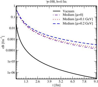
Figure 1: The variation of magnetic field with time in vacuum and in a thermally conducting medium at different chemical potentials for impact parameter $b=4$ fm and Lorentz factor $\gamma=100$.

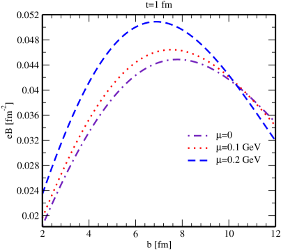
Figure 2: The variation of magnetic field with impact parameter in a thermally conducting medium for different values of chemical potential at time $t=1$ fm.

It can be observed that the strength of magnetic field decays very fast in the vacuum, whereas in an electrically conducting medium, its decay becomes much slower. Initially, the decrease in the strength of magnetic field in the thermal medium is noticeably high, however it gradually saturates with the time, which explains that, as compared to the strong magnetic field, the weak magnetic field can stay longer. In figure 1, we have also noticed that the presence of chemical potential in the medium helps in elongating the lifetime of magnetic field. Thus, the properties of a dense thermal medium are expected to be influenced by the magnetic field. However at initial time, the difference between the variations of magnetic field in two mediums at zero chemical potential and finite chemical potential is less conspicuous.

Figure 2 displays the variation of the strength of magnetic field with impact parameter at a fixed time $t=1$ fm for different values of chemical potential. It can be observed that the trend of variation of $eB$ with $b$ is not monotonic. It increases with $b$ peaking at $b$ values for mid-central collision and then it shows a gradual decrease. With the increase of chemical potential, the peak shifts towards lower $b$ values. Thus, for a larger chemical potential, the magnetic field attains its highest strength at a smaller impact parameter.

4 Results and discussions

In this section, we are going to discuss the results on different charge and heat transport coefficients by using the thermal masses of charged particles in the quasiparticle description. It should be noted that the relaxation time approximation of the Boltzmann transport equation does not include the interactions among the constituents of the medium. However, in the quasiparticle description, each parton acquires a quasipaticle/thermally generated mass, which basically incorporates the interactions of the concerned parton with other partons in the medium. In this description, the QGP medium is described as a medium consisting of thermally massive noninteracting quasipartons. The quasiparticle masses predominantly depend on temperature of the medium and for a dense thermal medium, they depend on chemical potential ($\mu_{f}$) too. The quasiparticle mass (squared) of the $f$th parton is given [83, 84] by

$$m_{fT}^{2}=\frac{g^{2}T^{2}}{6}\left(1+\frac{\mu_{f}^{2}}{\pi^{2}T^{2}}\right),$$ (51)

with $g^{2}=4\pi\alpha_{s}$, where $\alpha_{s}$ represents the one-loop strong running coupling constant at finite temperature, chemical potential and magnetic field and is defined in eq. (22). Here the magnetic field-dependence enters only through $\alpha_{s}$, at least in the weak magnetic field regime. The chemical potentials for all quark flavors are kept same, i.e. $\mu_{f}=\mu$.

The quasiparticle description does not change the form of the Boltzmann transport equation, however, it does change the equilibrium distribution function via the dispersion relation. In the Boltzmann transport equation (27), the term involving the electromagnetic/Lorentz force is $\mathbf{F}\cdot\left[\mathbf{v}\frac{\partial f_{f}}{\partial p_{0}}+\frac{\partial f_{f}}{\partial\mathbf{p}}\right]$, where the factors $\frac{\partial f_{f}}{\partial p_{0}}$ and $\frac{\partial f_{f}}{\partial\mathbf{p}}$ get affected by the quasiparticle description. It is important to note that the quasiparticle model describes the mutual interactions of the partons in the thermal medium, but not their response to an external force field, so, the Lorentz force ($\mathbf{F}$) remains unaltered. Thus, the overall effect of quasiparticle mass on the Boltzmann transport equation is encoded in the factors $\frac{\partial f_{f}}{\partial p_{0}}$ and $\frac{\partial f_{f}}{\partial\mathbf{p}}$. On the other hand, in effective mass models [85, 86], the terms concerning the mean field contribution had been added to the kinetic theory definition of the energy-momentum tensor. Similarly, the mean field term of the effective fugacity model of kinetic theory involves the fugacity parameters and their derivatives, and ref. [59] had reported that the mean field effects are negligible at high temperatures due to very slow variation of the effective fugacity with temperature. This suggests that, unlike effective mass models in which one needs to add terms concerning the mean field contribution to the kinetic theory [85, 86, 59], in our case of quasiparticle description, no additional mean field term is required, as the modified dispersions of the quasiparticles take care of the thermal mass effect in the Boltzmann transport equation of kinetic theory.

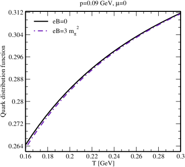
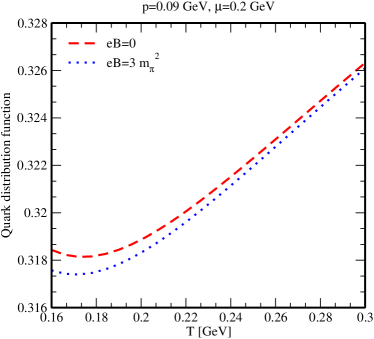
a	b

Figure 3: The quark distribution function as a function of temperature for a fixed momentum.

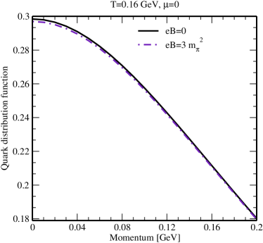
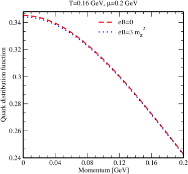
a	b

Figure 4: The quark distribution function as a function of momentum at a fixed temperature.

In the kinetic theory, the transport coefficients and their relative behavior mostly depend on the distribution function. So, before discussing the results on different transport coefficients, let us observe how the distribution function of $u$ quark varies with temperature and with momentum in the presence of weak magnetic field and finite chemical potential. The quark distribution function has been shown as a function of temperature in figure 3 and as a function of momentum in figure 4. It can be seen that the distribution function gets slightly decreased in the presence of a weak magnetic field in comparison to that in the pure thermal medium at zero magnetic field. However, a finite value of chemical potential significantly affects the magnitude and the shape of the distribution function (figures 3b and 4b) as compared to the zero chemical potential case (figures 3a and 4a). In the low temperature regime, the difference between the distribution functions at zero chemical potential and at finite chemical potential is larger. However, at high temperature, they tend to approach each other, as $\frac{\mu}{T}$ gets waned with the increase of temperature.

4.1 Components of charge transport

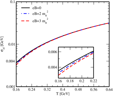
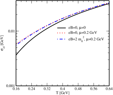
a	b

Figure 5: The variation of the electrical conductivity, $\sigma_{\rm el}$ with temperature (a) in the presence of weak magnetic field and (b) in the presence of finite chemical potential.

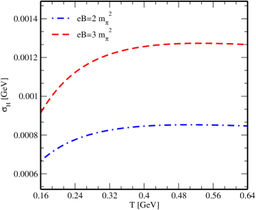
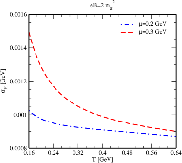
a	b

Figure 6: The variation of the Hall conductivity, $\sigma_{\rm H}$ with temperature (a) in the presence of weak magnetic field and (b) in the presence of finite chemical potential.

Figure 5 shows the variation of the electrical conductivity, $\sigma_{\rm el}$ as a function of the temperature in the presence of a weak magnetic field. In particular, figure 5a shows the variation of $\sigma_{\rm el}$ at zero chemical potential while figure 5b shows the same for finite chemical potential. It can be observed from figure 5a that the $\sigma_{\rm el}$ slightly decreases in the presence of a weak magnetic field when compared to zero magnetic field case at low temperatures. This observation can be related to the motion of electrically charged quarks in the hot QCD medium. According to the Ohm’s law, the electrical conductivity is directly proportional to the current along the direction of the electric field. But in the presence of a magnetic field, quarks experience a Lorentz force, which influences their direction of motion (of quarks) and results in a reduction of electric current in the direction of electric field, and hence a decrease in the electrical conductivity is observed. Figure 5b shows that the presence of a finite chemical potential results in the increase of $\sigma_{\rm el}$ in a weakly magnetized QCD medium. Thus, it is inferred that the weak magnetic field decreases the charge conduction in a hot QCD matter, whereas the finite chemical potential tends to increase it. This can be comprehended from the fact that, in the weak magnetic field regime, the energy scale associated with the magnetic field is smaller than other energy scales, so $\sigma_{\rm el}$ becomes more sensitive to the energy scale related to the chemical potential and it results in the increase of the charge transport at finite chemical potential even in the presence of a weak magnetic field. The behavior of $\sigma_{\rm el}$ is also modulated by the distribution function, because, according to the nonrelativistic Drude’s formula, the electrical conductivity is directly proportional to the number density, i.e. the integration of distribution function over momentum space. Thus, the decrease of $\sigma_{\rm el}$ due to weak magnetic field and its increase due to finite chemical potential can also be understood from the decrease of distribution function in a weak magnetic field and its increase at finite chemical potential (figures 3 and 4).

In figure 6, the variation of Hall conductivity, $\sigma_{\rm H}$ as a function of temperature is shown in the presence of weak magnetic field and finite chemical potential. It can be observed that, at $\mu=0$, $\sigma_{\rm H}$ shows increasing behavior with $T$ in the low temperature regime (figure 6a), which is mainly due to the increase of distribution function with $T$. On the other hand, $\sigma_{\rm H}$ shows decreasing behavior with $T$ at finite $\mu$ (figure 6b), which can be comprehended as follows. At finite $\mu$, the increase of distribution function with $T$ becomes smaller and the factor $\beta\tau_{f}^{2}$ ($\approx\frac{1}{T^{3}}$, at least in the weak magnetic field regime) appearing in the expression of $\sigma_{\rm H}$ (34) dominates, thus an overall decrease of $\sigma_{\rm H}$ with increasing $T$ is observed.

Hall conductivity vanishes at zero magnetic field, which can be understood from the presence of cyclotron frequency ($\omega_{c}$) in the numerator of eq. (34). With the increase of magnetic field, $\sigma_{\rm H}$ gets increased even in the weak magnetic field limit (figure 6a), unlike the case of $\sigma_{\rm el}$, because $\sigma_{\rm H}$ is directly related to $\omega_{c}$. Increase in the magnitude of $\sigma_{\rm H}$ is also observed with the increase of chemical potential (figure 6b), which can be inferred from the fact that, at finite chemical potential, difference in the numbers of particles and antiparticles produces a net Hall current which is proportional to the Hall conductivity.

4.2 Components of heat transport

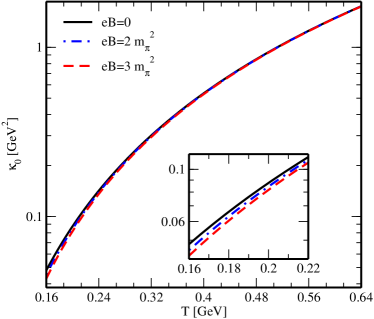
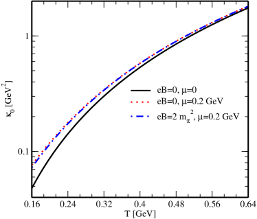
a	b

Figure 7: The variation of the thermal conductivity, $\kappa_{0}$ with temperature (a) in the presence of weak magnetic field and (b) in the presence of finite chemical potential.

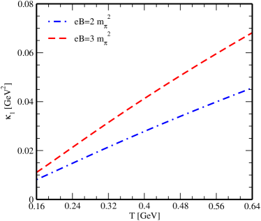
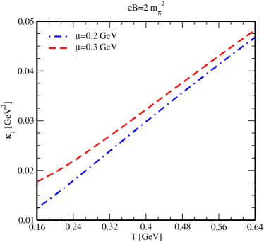
a	b

Figure 8: The variation of the Hall-type thermal conductivity, $\kappa_{1}$ with temperature (a) in the presence of weak magnetic field and (b) in the presence of finite chemical potential.

Figure 7 depicts the variation of the thermal conductivity, $\kappa_{0}$ with the temperature in the presence of a weak magnetic field. It can be observed that the presence of weak magnetic field reduces $\kappa_{0}$ and the reduction is larger at low temperatures (figure 7a). On the other hand, a finite chemical potential enhances the magnitude of $\kappa_{0}$ (figure 7b). However, this enhancement of $\kappa_{0}$ is not same over the entire range of temperature, rather it is more conspicuous at low temperatures. In figure 8, the Hall-type thermal conductivity, $\kappa_{1}$ is plotted as a function of temperature and it vanishes at zero magnetic field, which can be understood from eq. (48). Unlike $\kappa_{0}$, $\kappa_{1}$ directly depends on cyclotron frequency, so one can observe that the magnitude of $\kappa_{1}$ gets increased with the magnetic field even in the weak magnetic field regime (figure 8a). In addition, finite chemical potential also increases the magnitude of $\kappa_{1}$ (figure 8b). Both $\kappa_{0}$ and $\kappa_{1}$ are found to increase with $T$, but one would expect the reverse effect of $T$ on these conductivities due to the presence of terms $\beta^{2}\tau_{f}$ and $\beta^{2}\tau_{f}^{2}$ in the expressions of $\kappa_{0}$ (47) and $\kappa_{1}$ (48), respectively. However, in their expressions, the increase of enthalpy per particle and the increase of distribution function with $T$ somewhat compensate this effect and thus, we observe an overall increase of $\kappa_{0}$ and $\kappa_{1}$ with temperature.

In the strong magnetic field regime, there is a severe reduction of the phase space from (3+1)-dimensions to (1+1)-dimensions, so the charged particles are constrained to move along the direction of magnetic field. On the other hand, the weak magnetic field does not restrict the 3-dimensional dynamics and there exist different components of charge and heat transport coefficients. Thus, it may not be plausible to compare our results on conductivities in the weak magnetic field regime with that in the strong magnetic field regime at the equal base. However, we may roughly compare our results in the weak magnetic field with the results obtained in the strong magnetic field. For example, in ref. [54], $\sigma_{\rm el}$ was calculated using the quenched SU($2$) lattice gauge theory, where for the deconfinement phase, only the component of $\sigma_{\rm el}$ along the direction of magnetic field exists and it increases as the strength of magnetic field increases. According to the observation on $\sigma_{\rm el}$ which was calculated in ref. [31] using the Kubo formalism and the dilute instanton-liquid model, the effect of the external magnetic field was relatively considerable in the low temperature region $T\leq 200$ MeV. In ref. [55], $\sigma_{\rm el}$ was estimated using the real time formalism through the diagrammatic method and found to be much larger than its counterpart at zero magnetic field. The main reasons behind this large increment were the strong magnetic field and the smaller value of the current quark mass. In ref. [57], the Landau level resummation via kinetic equations has been implemented and a fixed QCD coupling ($\alpha_{s}=0.3$) was used in the evaluation of $\sigma_{\rm el}$, which has very large value in the lowest Landau level (LLL) approximation and remains almost insensitive to $\mu$, unlike our observation in weak magnetic field, where the effect of $\mu$ is noticeable. In ref. [13], electrical and thermal conductivities have been studied using the kinetic theory with the quasiparticle model in the strong magnetic field limit, where both the conductivities were found to be enhanced by the strong magnetic field, unlike our present work, where they get decreased in weak magnetic field as compared to their counterparts in the absence of magnetic field. The effective fugacity approach has also reported large magnitudes of $\sigma_{\rm el}$ ($\mathcal{O}(10^{2})$) [59] and $\kappa$ (between $\mathcal{O}(10^{1})$ to $\mathcal{O}(10^{2})$) [60] in the LLL approximation due to the presence of strong magnetic field. Our results in the weak magnetic field regime are totally different from the abovementioned results in the strong magnetic field regime. Main reasons behind this are the differences in relaxation times, phase spaces and distribution functions in both types of magnetic field regimes.

5 Applications

In this section, we study the effects of weak magnetic field and chemical potential on some applications of charge and heat transport coefficients. Subsections 5.1, 5.2 and 5.3 are devoted to observe the local equilibrium property of the medium through the Knudsen number, the elliptic flow and the relative behavior between the charge conduction and the heat conduction through the Wiedemann-Franz law, respectively.

5.1 Knudsen number

The Knudsen number, $\Omega$ is defined in terms of the mean free path ($\lambda$) and the characteristic length scale of the medium ($l$) as

$$\Omega=\frac{\lambda}{l}~{}.$$ (52)

If the mean free path is smaller than the characteristic length scale, then $\Omega$ is less than one and the equilibrium hydrodynamics is applicable. The mean free path can be calculated using $\kappa$ as

$$\lambda=\frac{3\kappa}{vC_{V}}~{},$$ (53)

where $C_{V}$ and $v$ represent the specific heat at constant volume and the relative speed, respectively. Thus, $\Omega$ takes the following form,

$$\Omega=\frac{3\kappa}{lvC_{V}}~{}.$$ (54)

Here, $C_{V}$ has been calculated from the energy-momentum tensor ($C_{V}=\partial(u_{\mu}T^{\mu\nu}u_{\nu})/\partial T$). In computing $\Omega$, we have fixed $v\simeq 1$ and $l=4$ fm. We note that, for two heat transport coefficients ($\kappa_{0}$ and $\kappa_{1}$) in a weak magnetic field, there also exist two components of the Knudsen number, such as $\Omega_{0}$ and $\Omega_{1}$.

a	b

Figure 9: The variations of (a) $\Omega_{0}$ and (b) $\Omega_{1}$ with temperature for different values of magnetic field and chemical potential.

Figure 9 shows the variations of the Knudsen number components $\Omega_{0}$ and $\Omega_{1}$ as functions of temperature. It can be seen that $\Omega_{0}$ lies much below unity in the absence of both magnetic field and chemical potential (figure 9a). The presence of weak magnetic field decreases $\Omega_{0}$, whereas the additional presence of chemical potential leads to an increase of this component of the Knudsen number. Similarly, $\Omega_{1}$ lies much below unity and is even smaller in magnitude as compared to $\Omega_{0}$. Like $\Omega_{0}$, $\Omega_{1}$ also increases with the rise of chemical potential. The observations on $\Omega_{0}$ and $\Omega_{1}$ at finite $eB$ and finite $\mu$ corroborate the observations on $\kappa_{0}$ (figure 7) and $\kappa_{1}$ (figure 8) in the similar environment. Both, $\Omega_{0}$ and $\Omega_{1}$ remain much less than unity over the entire range of temperature. It indicates that, there is sufficient separation between microscopic and macroscopic length scales of the medium and the hot QCD matter stays in local equilibrium even in the presence of both weak magnetic field and finite chemical potential. In all cases, $\Omega_{0}$ and $\Omega_{1}$ follow the decreasing trend with the rise of temperature, same as in the absence of magnetic field.

5.2 Elliptic flow

The elliptic flow coefficient, $v_{2}$ describes the azimuthal anisotropy in the momentum space of the produced particles in heavy ion collisions. This is a direct consequence of initial pressure gradients because of the initial spatial anisotropy and the interactions among the produced particles [87]. The elliptic flow is related to the Knudsen number by the following expression [88, 89, 90],

$$v_{2}=\frac{v_{2}^{h}}{1+\frac{\Omega}{\Omega_{h}}},$$ (55)

where $v_{2}^{h}$ is the value of elliptic flow in the hydrodynamic limit, i.e. $\Omega\rightarrow 0$ limit. We note that we have used $\Omega=\Omega_{0}$ here. The value of $\Omega_{h}$ can be obtained by observing the transition between the hydrodynamic regime and the free streaming particle regime. The presence of weak magnetic field as well as chemical potential could significantly affect the magnitude of elliptic flow. In our calculation, we have used $v_{2}^{h}\approx 0.1$ and $\Omega_{h}\approx 0.7$, which are obtained from the transport calculation in ref. [90].

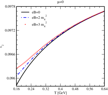
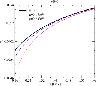
a	b

Figure 10: The elliptic flow coefficient, $v_{2}$ as a function of temperature (a) in the presence of weak magnetic field and (b) at finite chemical potential.

Figure 10 depicts the variation of elliptic flow as a function of temperature for weak magnetic field and finite chemical potential. It can be observed that $v_{2}$ increases with temperature. Figure 10a compares the temperature dependence of $v_{2}$ for different values of magnetic field. It can be seen that $v_{2}$ is higher for weak magnetic field at low temperatures. The increase is not uniform over the entire range of temperature. The $v_{2}$ approaches its value at zero magnetic field at higher temperatures, because the sensitivity of $v_{2}$ to the weak magnetic field decreases as the energy scale related to the temperature grows. The presence of the strong magnetic field also enhances the elliptic flow, as it has been reported in ref. [91]. The effect of finite chemical potential on the elliptic flow is displayed in figure 10b. The finite chemical potential decreases the magnitude of elliptic flow. The deviation of $v_{2}$ from its value at zero chemical potential is larger at lower temperatures and the convergence happens at higher temperatures.

As observed in figure 9, the Knudsen number becomes zero when the hydrodynamic limit is approached. In this case, $v_{2}$ becomes maximum and attains its hydrodynamic value. It can be inferred, that, as $\Omega$ decreases, the number of collisions increases which leads to a larger anisotropic flow, hence $v_{2}$ grows and eventually saturates when the medium reaches local equilibrium. One can also understand from eq. (55) that, for large $\Omega$ or far from the hydrodynamic limit, $v_{2}$ decreases like $1/\Omega$. The increase in $v_{2}$ at finite magnetic field can be comprehended as follows: The presence of magnetic field makes significant variations in the velocities of particles and the degree of variation depends on the angle between the direction of flow and the direction of magnetic field which impacts the development of anisotropy, thus, an increase in the elliptic flow is observed. To some extent, this enhancement of $v_{2}$ in the weak magnetic field regime can also be understood from the reduction of thermal conductivity (through the dependence on mean free path in eq. (53)) in the similar environment (figure 7a). However, with an increase of chemical potential, thermal conductivity increases (figure 7b), which results in the decrease of $v_{2}$ at finite chemical potential. Thus, the magnitude of $v_{2}$ acts as a probe to detect the level of thermalization in different scenarios. Quantitatively, for a temperature range of 0.16-0.64 GeV, our calculation gives the value of $v_{2}$ in the range 0.0958-0.0976 at $eB=0$, $\mu=0$, in the range 0.0946-0.0976 at $eB=0$, $\mu\neq 0$ and in the range 0.0962-0.0976 at $eB\neq 0$, $\mu=0$. The obtained values are closer to the experimental data of elliptic flow obtained from STAR collaboration at RHIC [92, 93] and ALICE collaboration at LHC [94] for $p_{T}\approx 1$ GeV.

5.3 Wiedemann-Franz law

According to the Wiedemann-Franz law, the ratio of the heat transport coefficient to the charge transport coefficient is directly proportional to the temperature, where the proportionality factor is the Lorenz number ($L$),

$$\frac{\kappa}{\sigma_{\rm el}}=LT~{}.$$ (56)

This law sheds light on the relative behavior of the charge transport and the heat transport in a medium. We note that, in weak magnetic field, there exist two components of the Lorenz number, such as $L_{0}$ and $L_{1}$,

$$L_{0}=\frac{\kappa_{0}}{\sigma_{\rm el}T}~{},$$ (57)

$$L_{1}=\frac{\kappa_{1}}{\sigma_{\rm H}T}~{}.$$ (58)

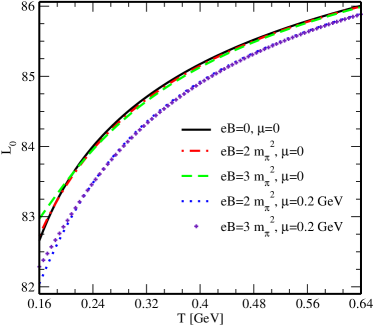
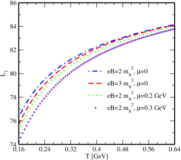
a	b

Figure 11: The variations of (a) $L_{0}$ and (b) $L_{1}$ with temperature for different values of magnetic field and chemical potential.

Figure 11 depicts the variations of the Lorenz number components $L_{0}$ and $L_{1}$ as functions of the temperature for various conditions of magnetic field and chemical potential. It can be observed that both $L_{0}$ and $L_{1}$ increase with $T$, i.e. the heat transport forges ahead of the charge transport. This indicates that the hot QCD matter does not comply with the Wiedemann-Franz law. Both $L_{0}$ and $L_{1}$ of the weakly magnetized medium almost follow the same trend as that of the zero magnetic field case with temperature. The presence of finite chemical potential in the magnetized medium reduces the magnitudes of $L_{0}$ and $L_{1}$ for all temperatures. However, throughout the variation, these components of the Lorenz number remain larger than unity, indicating that the thermal conductivity ($\kappa_{0}$) prevails over the electrical conductivity ($\sigma_{\rm el}$) and the Hall-type thermal conductivity ($\kappa_{1}$) also prevails over the Hall conductivity ($\sigma_{\rm H}$) at any value of the temperature. The observed enhanced difference between the heat transport and the charge transport is in accordance with the observations on charge conduction behavior in figures 5 and 6 and heat conduction behavior in figures 7 and 8.

6 Summary

The effects of weak magnetic field and finite chemical potential on the charge and heat transport properties of hot and dense QCD matter have been investigated. In the presence of magnetic field, the transport coefficients do not remain isotropic and they possess different components. The components of charge transport and heat transport, such as electrical conductivity ($\sigma_{\rm el}$), Hall conductivity ($\sigma_{\rm H}$), thermal conductivity ($\kappa_{0}$) and Hall-type thermal conductivity ($\kappa_{1}$) were determined by solving the relativistic Boltzmann transport equation within the relaxation time approximation of kinetic theory. A reduction in the magnitudes of $\sigma_{\rm el}$ and $\kappa_{0}$ and an enhancement in the magnitudes of $\sigma_{\rm H}$ and $\kappa_{1}$ with the increase of magnetic field were observed, whereas the emergence of finite chemical potential tends to increase all of their magnitudes. The transport coefficients were further used to study the Knudsen number, the elliptic flow and the Wiedemann-Franz law. The Knudsen number components in the weakly magnetized hot and dense QCD matter retain their values much below unity. Thus, there is sufficient separation between the mean free path and the characteristic length scale for the medium to remain in the local equilibrium state. The elliptic flow gets increased in the presence of the weak magnetic field, whereas the presence of finite chemical potential decreases it. The Lorenz number components in the Wiedemann-Franz law were found to be strongly affected by the chemical potential than by the weak magnetic field. However, with the increase of temperature, the Lorenz number components were observed to increase, confirming the violation of the Wiedemann-Franz law for hot and dense QCD matter in the presence of a weak magnetic field.

7 Acknowledgment

One of us (S. R.) would like to acknowledge the Indian Institute of Technology Bombay for the Institute postdoctoral fellowship.

Appendix A Derivation of equation (31)

By substituting the following partial derivatives in eq. (30),

$$v_{x}\frac{\partial f_{f}}{\partial p_{0}} = -\beta v_{x}f_{f}^{0}-qE\tau_{f}\beta f_{f}^{0}v_{x}^{2}\left(\frac{1}{\omega_{f}}+\beta\right)-\beta f_{f}^{0}\Gamma_{x}v_{x}^{2}\left(\frac{1}{\omega_{f}}+\beta\right)$$ (A.59)

$$-\beta f_{f}^{0}\Gamma_{y}v_{x}v_{y}\left(\frac{1}{\omega_{f}}+\beta\right)-\beta f_{f}^{0}\Gamma_{z}v_{x}v_{z}\left(\frac{1}{\omega_{f}}+\beta\right),$$

$$v_{x}\frac{\partial f_{f}}{\partial p_{y}} = -\beta v_{x}v_{y}f_{f}^{0}-qE\tau_{f}\beta f_{f}^{0}v_{x}^{2}v_{y}\left(\frac{1}{\omega_{f}}+\beta\right)-\beta f_{f}^{0}\Gamma_{x}v_{x}^{2}v_{y}\left(\frac{1}{\omega_{f}}+\beta\right)$$ (A.60)

$$-\beta f_{f}^{0}\Gamma_{y}v_{x}v_{y}^{2}\left(\frac{1}{\omega_{f}}+\beta\right)+\frac{v_{x}\Gamma_{y}\beta f_{f}^{0}}{\omega_{f}}-\beta f_{f}^{0}\Gamma_{z}v_{x}v_{y}v_{z}\left(\frac{1}{\omega_{f}}+\beta\right),$$

$$v_{y}\frac{\partial f_{f}}{\partial p_{x}} = -\beta v_{y}v_{x}f_{f}^{0}-qE\tau_{f}\beta f_{f}^{0}v_{y}v_{x}^{2}\left(\frac{1}{\omega_{f}}+\beta\right)+\frac{qE\tau_{f}\beta f_{f}^{0}v_{y}}{\omega_{f}}$$ (A.61)

$$-\beta f_{f}^{0}\Gamma_{x}v_{y}v_{x}^{2}\left(\frac{1}{\omega_{f}}+\beta\right)+\frac{\Gamma_{x}\beta f_{f}^{0}v_{y}}{\omega_{f}}-\beta f_{f}^{0}\Gamma_{y}v_{y}^{2}v_{x}\left(\frac{1}{\omega_{f}}+\beta\right)$$

$$-\beta f_{f}^{0}\Gamma_{z}v_{y}v_{z}v_{x}\left(\frac{1}{\omega_{f}}+\beta\right),$$

and then dropping higher order velocity terms, we get

$$-qE\tau_{f}v_{x}+\left(\Gamma_{x}v_{x}+\Gamma_{y}v_{y}+\Gamma_{z}v_{z}\right)-\frac{qB\tau_{f}}{\omega_{f}}\left(v_{x}\Gamma_{y}-v_{y}\Gamma_{x}\right)+\frac{\tau_{f}^{2}qBqEv_{y}}{\omega_{f}}=0.$$ (A.62)

Comparing the coefficients of $v_{z}$ on both sides of eq. (A.62), we get $\Gamma_{z}=0$. Then, we have

$$-qEv_{x}+\frac{\Gamma_{x}}{\tau_{f}}v_{x}-\omega_{c}\Gamma_{y}v_{x}+\frac{\Gamma_{y}}{\tau_{f}}v_{y}+\omega_{c}\Gamma_{x}v_{y}+\tau_{f}\omega_{c}qEv_{y}=0,$$ (A.63)

where the cyclotron frequency, $\omega_{c}=\frac{qB}{\omega_{f}}$. Equating coefficients of $v_{x}$ and $v_{y}$ on both sides of eq. (A.63), we get

$$\frac{\Gamma_{x}}{\tau_{f}}-\omega_{c}\Gamma_{y}-qE=0,$$ (A.64)

$$\frac{\Gamma_{y}}{\tau_{f}}+\omega_{c}\Gamma_{x}+\tau_{f}\omega_{c}qE=0.$$ (A.65)

After solving equations (A.64) and (A.65), we obtain

$$\Gamma_{x}=\frac{qE\tau_{f}\left(1-\omega_{c}^{2}\tau_{f}^{2}\right)}{1+\omega_{c}^{2}\tau_{f}^{2}},$$ (A.66)

$$\Gamma_{y}=-\frac{2qE\omega_{c}\tau_{f}^{2}}{1+\omega_{c}^{2}\tau_{f}^{2}}.$$ (A.67)

Now, ansatz (29) can be written as

$$f_{f}=f_{f}^{0}-qE\tau_{f}\frac{\partial f_{f}^{0}}{\partial p_{x}}-qE\tau_{f}\left(\frac{1-\omega_{c}^{2}\tau_{f}^{2}}{1+\omega_{c}^{2}\tau_{f}^{2}}\right)\frac{\partial f_{f}^{0}}{\partial p_{x}}+2qE\left(\frac{\omega_{c}\tau_{f}^{2}}{1+\omega_{c}^{2}\tau_{f}^{2}}\right)\frac{\partial f_{f}^{0}}{\partial p_{y}}.$$ (A.68)

By using $\frac{\partial f_{f}^{0}}{\partial p_{x}}=v_{x}\frac{\partial f_{f}^{0}}{\partial\omega_{f}}=-v_{x}\beta f_{f}^{0}\left(1-f_{f}^{0}\right)$ and $\frac{\partial f_{f}^{0}}{\partial p_{y}}=v_{y}\frac{\partial f_{f}^{0}}{\partial\omega_{f}}=-v_{y}\beta f_{f}^{0}\left(1-f_{f}^{0}\right)$, eq. (A.68) gets simplified into

$$f_{f} = f_{f}^{0}+qE\tau_{f}v_{x}\beta f_{f}^{0}\left(1-f_{f}^{0}\right)+qE\tau_{f}v_{x}\beta\left(\frac{1-\omega_{c}^{2}\tau_{f}^{2}}{1+\omega_{c}^{2}\tau_{f}^{2}}\right)f_{f}^{0}\left(1-f_{f}^{0}\right)$$ (A.69)

$$-2qEv_{y}\beta\left(\frac{\omega_{c}\tau_{f}^{2}}{1+\omega_{c}^{2}\tau_{f}^{2}}\right)f_{f}^{0}\left(1-f_{f}^{0}\right).$$

This leads to the determination of $\delta f_{f}$ as

$$\delta f_{f}=2qEv_{x}\beta\left(\frac{\tau_{f}}{1+\omega_{c}^{2}\tau_{f}^{2}}\right)f_{f}^{0}\left(1-f_{f}^{0}\right)-2qEv_{y}\beta\left(\frac{\omega_{c}\tau_{f}^{2}}{1+\omega_{c}^{2}\tau_{f}^{2}}\right)f_{f}^{0}\left(1-f_{f}^{0}\right).$$ (A.70)

Appendix B Derivation of equation (45)

Substituting the value of $L$ (44) in eq. (43) and simplifying, we have

$$\frac{\left(\omega_{f}-h_{f}\right)}{T}v_{x}\left(\partial^{x}T-\frac{T}{nh_{f}}\partial^{x}P\right)+\frac{\Gamma_{x}v_{x}}{\tau_{f}}-\omega_{c}\Gamma_{y}v_{x}-qEv_{x}$$

$$+\frac{\left(\omega_{f}-h_{f}\right)}{T}v_{y}\left(\partial^{y}T-\frac{T}{nh_{f}}\partial^{y}P\right)+\frac{\Gamma_{y}v_{y}}{\tau_{f}}+\omega_{c}\Gamma_{x}v_{y}+\tau_{f}\omega_{c}qEv_{y}$$

$$+p_{0}\frac{DT}{T}-\frac{p^{\mu}p^{\alpha}}{p_{0}}\nabla_{\mu}u_{\alpha}+TD\left(\frac{\mu_{f}}{T}\right)=0.$$ (B.71)

Equating the coefficients of $v_{x}$ and $v_{y}$ on both sides of the above equation, we obtain

$$\frac{\left(\omega_{f}-h_{f}\right)}{T}\left(\partial^{x}T-\frac{T}{nh_{f}}\partial^{x}P\right)+\frac{\Gamma_{x}}{\tau_{f}}-\omega_{c}\Gamma_{y}-qE=0,$$ (B.72)

$$\frac{\left(\omega_{f}-h_{f}\right)}{T}\left(\partial^{y}T-\frac{T}{nh_{f}}\partial^{y}P\right)+\frac{\Gamma_{y}}{\tau_{f}}+\omega_{c}\Gamma_{x}+\tau_{f}\omega_{c}qE=0.$$ (B.73)

By solving equations (B.72) and (B.73), $\Gamma_{x}$ and $\Gamma_{y}$ are respectively determined as

$$\Gamma_{x} = \frac{qE\tau_{f}\left(1-\omega_{c}^{2}\tau_{f}^{2}\right)}{1+\omega_{c}^{2}\tau_{f}^{2}}-\frac{\tau_{f}\left(\omega_{f}-h_{f}\right)}{T\left(1+\omega_{c}^{2}\tau_{f}^{2}\right)}\left(\partial^{x}T-\frac{T}{nh_{f}}\partial^{x}P\right)$$ (B.74)

$$-\frac{\omega_{c}\tau_{f}^{2}\left(\omega_{f}-h_{f}\right)}{T\left(1+\omega_{c}^{2}\tau_{f}^{2}\right)}\left(\partial^{y}T-\frac{T}{nh_{f}}\partial^{y}P\right),$$

$$\Gamma_{y} = -\frac{2\omega_{c}\tau_{f}^{2}qE}{1+\omega_{c}^{2}\tau_{f}^{2}}-\frac{\tau_{f}\left(\omega_{f}-h_{f}\right)}{T\left(1+\omega_{c}^{2}\tau_{f}^{2}\right)}\left(\partial^{y}T-\frac{T}{nh_{f}}\partial^{y}P\right)$$ (B.75)

$$+\frac{\omega_{c}\tau_{f}^{2}\left(\omega_{f}-h_{f}\right)}{T\left(1+\omega_{c}^{2}\tau_{f}^{2}\right)}\left(\partial^{x}T-\frac{T}{nh_{f}}\partial^{x}P\right).$$

Using the values of $\Gamma_{x}$ and $\Gamma_{y}$ in ansatz (29) and then simplifying, we get the infinitesimal change of the quark distribution function as

$$\delta f_{f} = \frac{2qE\tau_{f}v_{x}\beta f_{f}^{0}\left(1-f_{f}^{0}\right)}{1+\omega_{c}^{2}\tau_{f}^{2}}-\frac{2qE\omega_{c}\tau_{f}^{2}v_{y}\beta f_{f}^{0}\left(1-f_{f}^{0}\right)}{1+\omega_{c}^{2}\tau_{f}^{2}}-\beta^{2}f_{f}^{0}\left(1-f_{f}^{0}\right)\frac{\tau_{f}(\omega_{f}-h_{f})}{\left(1+\omega_{c}^{2}\tau_{f}^{2}\right)}$$ (B.76)

$$\times\left[v_{x}\left(\partial^{x}T-\frac{T}{nh_{f}}\partial^{x}P\right)+v_{y}\left(\partial^{y}T-\frac{T}{nh_{f}}\partial^{y}P\right)\right]-\beta^{2}f_{f}^{0}\left(1-f_{f}^{0}\right)$$

$$\times\frac{\omega_{c}\tau_{f}^{2}(\omega_{f}-h_{f})}{\left(1+\omega_{c}^{2}\tau_{f}^{2}\right)}\left[v_{x}\left(\partial^{y}T-\frac{T}{nh_{f}}\partial^{y}P\right)-v_{y}\left(\partial^{x}T-\frac{T}{nh_{f}}\partial^{x}P\right)\right].$$

References

- [1] V. Skokov, A. Illarionov, and V. Toneev, Int. J. Mod. Phys. A 24, 5925 (2009).
- [2] A. Bzdak and V. Skokov, Phys. Lett. B 710, 171 (2012).
- [3] K. Fukushima, D. E. Kharzeev and H. J. Warringa, Phys. Rev. D 78, 074033 (2008).
- [4] D. E. Kharzeev, L. D. McLerran and H. J. Warringa, Nucl. Phys. A 803, 227 (2008).
- [5] V. Braguta, M. N. Chernodub, V. A. Goy, K. Landsteiner, A. V. Molochkov and M. I. Polikarpov, Phys. Rev. D 89, 074510 (2014).
- [6] M. N. Chernodub, A. Cortijo, A. G. Grushin, K. Landsteiner and M. A. H. Vozmediano, Phys. Rev. B 89, 081407 (R) (2014).
- [7] D. E. Kharzeev, Prog. Part. Nucl. Phys. 75, 133 (2014).
- [8] D. Satow, Phys. Rev. D 90, 034018 (2014).
- [9] S. Pu, S. Y. Wu and D. L. Yang, Phys. Rev. D 91, 025011 (2015).
- [10] D. E. Kharzeev and D. T. Son, Phys. Rev. Lett. 106, 062301 (2011).
- [11] K. Tuchin, Adv. High Energy Phys. 2013, 490495 (2013).
- [12] L. McLerran and V. Skokov, Nucl. Phys. A 929, 184 (2014).
- [13] S. Rath and B. K. Patra, Phys. Rev. D 100, 016009 (2019).
- [14] S. Rath and B. K. Patra, J. High Energy Phys. 1712, 098 (2017).
- [15] A. Bandyopadhyay, B. Karmakar, N. Haque and M. G. Mustafa, Phys. Rev. D 100, 034031 (2019).
- [16] S. Rath and B. K. Patra, Eur. Phys. J. A 55, 220 (2019).
- [17] B. Karmakar, R. Ghosh, A. Bandyopadhyay, N. Haque and M. G. Mustafa, Phys. Rev. D 99, 094002 (2019).
- [18] H. van Hees, C. Gale, R. Rapp, Phys. Rev. C 84, 054906 (2011).
- [19] C. Shen, U. W. Heinz, J.-F. Paquet, C. Gale, Phys. Rev. C 89, 044910 (2014).
- [20] K. Tuchin, Phys. Rev. C 88, 024910 (2013).
- [21] K. A. Mamo, J. High Energy Phys. 1308, 083 (2013).
- [22] K. Fukushima, K. Hattori, H.-U. Yee and Y. Yin, Phys. Rev. D 93, 074028 (2016).
- [23] V. Roy, S. Pu, L. Rezzolla, and D. Rischke, Phys. Lett. B 750, 45 (2015).
- [24] G. Inghirami, L. Del Zanna, A. Beraudo, M. H. Moghaddam, F. Becattini and M. Bleicher, Eur. Phys. J. C 76, 659 (2016).
- [25] J. I. Kapusta and J. M. Torres-Rincon, Phys. Rev. C 86, 054911 (2012).
- [26] G. S. Denicol, H. Niemi, I. Bouras, E. Molnár, Z. Xu, D. H. Rischke, and C. Greiner, Phys. Rev. D 89, 074005 (2014).
- [27] A. Muronga, Phys. Rev. C 76, 014910 (2007).
- [28] A. Puglisi, S. Plumari and V. Greco, Phys. Rev. D 90, 114009 (2014).
- [29] L. Thakur, P. K. Srivastava, G. P. Kadam, M. George and H. Mishra, Phys. Rev. D 95, 096009 (2017).
- [30] S. Yasui and S. Ozaki, Phys. Rev. D 96, 114027 (2017).
- [31] Seung-il Nam, Phys. Rev. D 86, 033014 (2012).
- [32] M. Greif, I. Bouras, C. Greiner and Z. Xu, Phys. Rev. D 90, 094014 (2014).
- [33] B. Feng, Phys. Rev. D 96, 036009 (2017).
- [34] S. Mitra and V. Chandra, Phys. Rev. D 94, 034025 (2016).
- [35] S. Mitra and V. Chandra, Phys. Rev. D 96, 094003 (2017).
- [36] S. Gupta, Phys. Lett. B 597, 57 (2004).
- [37] G. Aarts, C. Allton, A. Amato, P. Giudice, S. Hands and J.-I. Skullerud, J. High Energy Phys. 1502, 186 (2015).
- [38] H.-T. Ding, O. Kaczmarek and F. Meyer, Phys. Rev. D 94, 034504 (2016).
- [39] E. M. Lifshitz and L. P. Pitaevskii, “Physical Kinetics”, Pergamon Press, 1981.
- [40] A. Harutyunyan and A. Sedrakian, Phys. Rev. C 94, 025805 (2016).
- [41] G. S. Denicol et al., Phys. Rev. D 98, 076009 (2018).
- [42] A. Das, H. Mishra and R. K. Mohapatra, Phys. Rev. D 101, 034027 (2020).
- [43] Z. Chen, C. Greiner, A. Huang and Z. Xu, Phys. Rev. D 101, 056020 (2020).
- [44] A. Das, H. Mishra and R. K. Mohapatra, Phys. Rev. D 99, 094031 (2019).
- [45] A. Das, H. Mishra and R. K. Mohapatra, Phys. Rev. D 100, 114004 (2019).
- [46] A. Dash, S. Samanta, J. Dey, U. Gangopadhyaya, S. Ghosh and V. Roy, Phys. Rev. D 102, 016016 (2020).
- [47] A. Bandyopadhyay, S. Ghosh, R. L. S. Farias, J. Dey and G. Krein, Phys. Rev. D 102, 114015 (2020).
- [48] B. Chatterjee, R. Rath, G. Sarwar, R. Sahoo, Eur. Phys. J. A 57, 45 (2021).
- [49] J. Dey, S. Satapathy, P. Murmu and S. Ghosh, Pramana - J. Phys. 95, 125 (2021).
- [50] S. Satapathy, S. Ghosh and S. Ghosh, Phys. Rev. D 104, 056030 (2021).
- [51] J. Dey, S. Satapathy, A. Mishra, S. Paul and S. Ghosh, Int. J. Mod. Phys. E 30, 2150044 (2021).
- [52] E. G. Blackman and G. B. Field, Phys. Rev. Lett. 71, 3481 (1993).
- [53] N. Bessho and A. Bhattacharjee, Phys. Plasmas 14, 056503 (2007).
- [54] P. V. Buividovich, M. N. Chernodub, D. E. Kharzeev, T. Kalaydzhyan, E. V. Luschevskaya and M. I. Polikarpov, Phys. Rev. Lett. 105, 132001 (2010).
- [55] K. Hattori and D. Satow, Phys. Rev. D 94, 114032 (2016).
- [56] L. Thakur and P. K. Srivastava, Phys. Rev. D 100, 076016 (2019).
- [57] K. Fukushima and Y. Hidaka, Phys. Rev. Lett. 120, 162301 (2018).
- [58] S. Rath and B. K. Patra, Eur. Phys. J. C 80, 747 (2020).
- [59] M. Kurian and V. Chandra, Phys. Rev. D 99, 116018 (2019).
- [60] M. Kurian, S. Mitra, S. Ghosh and V. Chandra, Eur. Phys. J. C 79, 134 (2019).
- [61] K. Fukushima, Phys. Lett. B 591, 277 (2004).
- [62] S. K. Ghosh, T. K. Mukherjee, M. G. Mustafa and R. Ray, Phys. Rev. D 73, 114007 (2006).
- [63] H. Abuki and K. Fukushima, Phys. Lett. B 676, 57 (2009).
- [64] N. Su and K. Tywoniuk, Phys. Rev. Lett. 114, 161601 (2015).
- [65] W. Florkowski, R. Ryblewski, N. Su and K. Tywoniuk, Phys. Rev. C 94, 044904 (2016).
- [66] S. Rath and B. K. Patra, Phys. Rev. D 102, 036011 (2020).
- [67] S. Rath and B. K. Patra, Eur. Phys. J. C 81, 139 (2021).
- [68] V. M. Bannur, J. High Energy Phys. 0709, 046 (2007).
- [69] V. M. Bannur, Phys. Rev. C 75, 044905 (2007).
- [70] P. K. Srivastava, S. K. Tiwari and C. P. Singh, Phys. Rev. D 82, 014023 (2010).
- [71] P. K. Srivastava and C. P. Singh, Phys. Rev. D 85, 114016 (2012).
- [72] Y. Hirono, M. Hongo and T. Hirano, Phys. Rev. C 90, 021903 (2014).
- [73] J. I. Kapusta, B. Müller and M. Stephanov, Phys. Rev. C 85, 054906 (2012).
- [74] C. Crecignani and G. M. Kremer, “The Relativistic Boltzmann Equation: Theory and Applications” (Boston, Birkhiiuser, 2002).
- [75] G. S. Rocha, G. S. Denicol and J. Noronha, Phys. Rev. Lett. 127, 042301 (2021).
- [76] L. D. Landau and E. M. Lifshitz, “Fluid Mechanics”, Pergamon Press, 1987.
- [77] K. Hattori, S. Li, D. Satow and H.-U. Yee, Phys. Rev. D 95, 076008 (2017).
- [78] K. Hattori, X.-G. Huang, D. H. Rischke and D. Satow, Phys. Rev. D 96, 094009 (2017).
- [79] M. Kurian and V. Chandra, Phys. Rev. D 97, 116008 (2018).
- [80] A. Hosoya and K. Kajantie, Nucl. Phys. B 250, 666 (1985).
- [81] A. Ayala et al., Phys. Rev. D 98, 031501 (2018).
- [82] M. Greif, F. Reining, I. Bouras, G. S. Denicol, Z. Xu and C. Greiner, Phys. Rev. E 87, 033019 (2013).
- [83] E. Braaten and R. D. Pisarski, Phys. Rev. D 45, R1827 (1992).
- [84] A. Peshier, B. Kämpfer and G. Soff, Phys. Rev. D 66, 094003 (2002).
- [85] K. Dusling and T. Schäfer, Phys. Rev. C 85, 044909 (2012).
- [86] M. Alqahtani, M. Nopoush and M. Strickland, Phys. Rev. C 95, 034906 (2017).
- [87] J. Y. Ollitrault, Phys. Rev. D 46, 229 (1992).
- [88] R. S. Bhalerao, J.-P. Blaizot, N. Borghini, J.-Y. Ollitrault, Phys. Lett. B 627, 49 (2005).
- [89] H.-J. Drescher, A. Dumitru, C. Gombeaud and J.-Y. Ollitrault, Phys. Rev. C 76, 024905 (2007).
- [90] C. Gombeaud and J.-Y. Ollitrault, Phys. Rev. C 77, 054904 (2008).
- [91] R. K. Mohapatra, P. S. Saumia and A. M. Srivastava, Mod. Phys. Lett. A 26, 2477 (2011).
- [92] R. Snellings (STAR collaboration), Acta Phys. Hung. A 21, 237 (2004).
- [93] A. Tang (STAR collaboration), arXiv:0808.2144 [nucl-ex].
- [94] K. Aamodt et al. (ALICE collaboration), Phys. Rev. Lett. 105, 252302 (2010).