Propagation and blocking in a two-patch reaction-diffusion model

Abstract

This paper is concerned with propagation phenomena for the solutions of the Cauchy problem associated with a two-patch one-dimensional reaction-diffusion model. It is assumed that each patch has a relatively well-defined structure which is considered as homogeneous. A coupling interface condition between the two patches is involved. We first study the spreading properties of solutions in the case when the per capita growth rate in each patch is maximal at low densities, a configuration which we call the KPP-KPP case, and which turns out to have some analogies with the homogeneous KPP equation in the whole line. Then, in the KPP-bistable case, we provide various conditions under which the solutions show different dynamics in the bistable patch, that is, blocking, virtual blocking (propagation with speed zero), or spreading with positive speed. Moreover, when propagation occurs with positive speed, a global stability result is proved. Finally, the analysis in the KPP-bistable frame is extended to the bistable-bistable case. AMS Subject Classifications: 35B40; 35C07; 35K57. Keywords: Patchy landscapes; Spreading speeds; Blocking; Propagation; Reaction-diffusion equations. The manuscript has no associated data.

1 Introduction

Propagation and propagation failure are two fundamental phenomena of great importance to many fields of science. For example, signal propagation in nerve cells occurs when the medium is homogeneous but can fail when inhomogeneities are present, such as a change in cross-sectional area, junctions to several other cells, or localized regions of reduced excitability [43, 36]. The mathematical framework of choice for modeling such phenomena are reaction-diffusion equations. In the simplest case, space is one-dimensional and inhomogeneities are represented as spatial changes in diffusivity or reaction terms at a single location, within a bounded region, or at periodically repeating locations. Our work here is inspired by the ecological dynamics of invasive species. When such species spread across a landscape, they encounter different habitat types, and their movement behavior as well as population dynamics may change according to landscape type. Our work is based on recent progress in modeling individual movement behaviors around interfaces where the landscape type changes [40] and continues the rigorous analysis of propagation phenomena in such models [28, 44].

Specifically, we consider a one-dimensional infinite landscape comprised of two semi-infinite patches. We denote $(-\infty,0)$ as patch 1 and $(0,+\infty)$ as patch 2. The interface that separates the two patches occurs at $x=0$. Our model consists of a reaction-diffusion equation for the species’ density on each patch and conditions that match the density and flux across the interface. We assume that each patch is homogeneous but the two patches may differ, so that the diffusion coefficients and the reaction terms (i.e. net population growth rates) may differ. Whereas most existing models for propagation and propagation failure assume that the population dynamics outside of a bounded region are identical, we are explicitly interested in the case where the dynamics differ, qualitatively and quantitatively, between the two patches. Hence, on each patch, the population density $\widetilde{u}=\widetilde{u}(t,x)$ satisfies an equation of the form

$$\widetilde{u}_{t}=d_{i}\widetilde{u}_{xx}+\widetilde{f}_{i}(\widetilde{u}),$$

where $i=1,2$, depending on patch type. Since we want the interface to be neutral with respect to reaction dynamics (i.e. no individuals are born or die from crossing the interface), the density flux is continuous at the interface, i.e., $d_{1}\widetilde{u}_{x}(t,0^{-})=d_{2}\widetilde{u}_{x}(t,0^{+})$. Continuity of the flux implies mass conservation in the absence of reaction terms. Individuals at the interface may show a preference for one or the other patch type. We denote this preference by $\alpha\in(0,1)$, where $\alpha>0.5$ indicates a preference for patch 1 and $\alpha<0.5$ for patch 2. Then the population density may be discontinuous at the interface with

$$(1-\alpha)d_{1}\widetilde{u}(t,0^{-})=\alpha d_{2}\widetilde{u}(t,0^{+}).$$

Please see [40] for a detailed derivation of this condition from a random walk and a thorough discussion of the biological implications. (A second case exists where both diffusion constants appear under square roots [40]; the theory developed below applies to that case as well.)

The discontinuity of the density at $x=0$ creates some difficulties in the analysis of propagation phenomena in our equations. It turns out to be much easier to scale the equations (by setting $u(t,x)=\widetilde{u}(t,x)$ in patch 1, $u(t,x)=k\widetilde{u}(t,x)$ in patch 2 with $k=\frac{\alpha}{1-\alpha}\,\frac{d_{2}}{d_{1}}$, $f_{1}=\widetilde{f}_{1}$ and $f_{2}(s)=k\widetilde{f}_{2}(s/k)$) so that the density is continuous; see [28] for details. Hence, in the present paper, we study the following equivalent two-patch problem:

$$\begin{cases}u_{t}=d_{1}u_{xx}+f_{1}(u),~{}~{}&t>0,\ x<0,\\ u_{t}=d_{2}u_{xx}+f_{2}(u),~{}~{}&t>0,\ x>0,\cr u(t,0^{-})=u(t,0^{+}),~{}~{}&t>0,\cr u_{x}(t,0^{-})=\sigma u_{x}(t,0^{+}),~{}~{}&t>0.\end{cases}$$ (1.1)

Here, the density is continuous across the interface but its derivative is not. The diffusion constants are assumed positive. Parameter $\sigma=(1-\alpha)/\alpha>0$ is related to $\alpha$, the probability that an individual at the interface chooses to move to patch 1. Please see Section 2.5 for more biological background and some interpretation of our results. Throughout this work, we assume that the functions $f_{i}$ $(i=1,2)$ are of class $C^{1}(\mathbb{R})$ and that

$$\exists\,K_{i}>0,\ \ f_{i}(0)=f_{i}(K_{i})=0\ \hbox{ and }\ f_{i}\leq 0\hbox{ in }[K_{i},+\infty).$$ (1.2)

Our analysis and results will depend on a few characteristic properties of the functions $f_{i}$. We distinguish between the Fisher-KPP type and the bistable type. We give precise definitions of these properties below in (1.4) and (1.7), respectively.

In [28], we analyzed in full detail the well-posedness problem for a related patch model in a one-dimensional spatially periodic habitat and also the spatial dynamics of the solution for the Cauchy problem under certain hypotheses on the reaction terms. Our goal of the present paper is to study spreading properties and propagation vs. blocking phenomena for the solutions of this two-patch model for various combinations of the reaction terms. Specifically, we investigate:

1. the asymptotic spreading properties of the solutions to the Cauchy problem (1.1) with compactly supported initial data when both reaction terms are of KPP type;

2. conditions for the solutions to the Cauchy problem (1.1) with compactly supported initial data to be blocked or to propagate with positive or zero speed when one reaction term is of KPP type and the other of bistable type; we also study the stability of a traveling wave in the bistable patch;

3. the asymptotic dynamics when both reaction terms are of bistable type.

Previous work on action potentials in nerve cells obtained some propagation and stability results when the reaction terms in both patches are identical and of bistable type and when the derivative is continuous at the interface, i.e., $\sigma=1$ [43]. We also mention recent work on a bistable equation in multiple (three or more) disjoint half-lines with a junction [32]: the existence of entire (defined for all times $t\in\mathbb{R}$) solutions is proved and blocking phenomena of entire solutions caused by the emergence of certain stationary solutions are investigated.

Before we state our main results, we summarize some relevant results on the classical homogeneous reaction-diffusion equation

$$u_{t}=u_{xx}+f(u),~{}~{}t>0,~{}x\in\mathbb{R},$$ (1.3)

where $f$ is a $C^{1}(\mathbb{R})$ function satisfying $f(0)=f(1)=0$. This equation has been extensively studied in the mathematical, physical and biological literature since the pioneering works of Fisher [24] and Kolmogorov, Petrovskii and Piskunov [34] on population genetics. We say that $f$ is of Fisher-KPP type (or simply KPP type) if

$$f(0)=f(1)=0\ \hbox{ and }\ 0<f(s)\leq f^{\prime}(0)s\ \hbox{ for all }\ s\in(0,1).$$ (1.4)

If $f$ in (1.3) is of KPP type, (1.3) admits traveling front solutions $u(t,x)=\varphi_{c}(x\cdot e-ct)$ with $\varphi_{c}:\mathbb{R}\to(0,1)$ and $\varphi_{c}(-\infty)=1$, $\varphi_{c}(+\infty)=0$, if and only if $c\geq c^{*}=2\sqrt{f^{\prime}(0)}$, where $e=\pm 1$ denotes the direction of propagation and $c$ is the speed. For each $c\geq c^{*}$, $\varphi_{c}$ satisfies

$$\varphi_{c}^{\prime\prime}+c\varphi_{c}^{\prime}+f(\varphi_{c})=0~{}\text{in}~{}\mathbb{R},~{}~{}\varphi_{c}^{\prime}<0~{}\text{in}~{}\mathbb{R},~{}~{}\varphi_{c}(-\infty)=1,~{}~{}\varphi_{c}(+\infty)=0,$$ (1.5)

and it is unique up to shifts. Moreover, there holds

$$\varphi_{c}(s)\mathop{\sim}_{s\to+\infty}\begin{cases}Ae^{-\lambda_{c}s}&\hbox{if }c>c^{*},\\ A^{*}se^{-\lambda_{c}s}&\hbox{if }c=c^{*},\\ \end{cases}$$ (1.6)

where $A,\,A^{*}$ are positive constants and the decay rate $\lambda_{c}>0$ is obtained from the linearized equation $u_{t}=u_{xx}+f^{\prime}(0)u$ and is given by $\lambda_{c}=\big{(}c-\sqrt{c^{2}-4f^{\prime}(0)}\big{)}/2$. It was proved in [12, 30, 35, 45] that the front with minimal speed $c^{*}$ attracts, in some sense, the solutions of the Cauchy problem (1.3) associated with nonnegative bounded nontrivial compactly supported initial data $u_{0}=u(0,\cdot)$. Furthermore, Aronson and Weinberger [4] proved that if $0\leq u\leq 1$ is the solution to the Cauchy problem (1.3) with a nontrivial compactly supported initial datum $0\leq u_{0}\leq 1$, then $\sup_{\mathbb{R}\backslash(-ct,ct)}u(t,\cdot)\to 0$ as $t\to+\infty$ for every $c>c^{*}$, and $\inf_{[-ct,ct]}u(t,\cdot)\to 1$ as $t\to+\infty$ for every $c\in[0,c^{*})$. We refer to these results as spreading properties. The minimal speed of traveling fronts, $c^{*}$, can therefore also be thought of as the asymptotic spreading speed.

In contrast, in the bistable case, defined as

$$f(0)\!=\!f(\theta)\!=\!f(1)\!=\!0\hbox{ for some $\theta\in(0,1)$, $f^{\prime}(0)<0$, $f^{\prime}(1)<0$, $f<0$ in $(0,\theta)$, $f>0$ in $(\theta,1)$},$$ (1.7)

equation (1.3) has traveling front solutions $u(t,x)=\phi(x\cdot e-ct)$, where $\phi:\mathbb{R}\to(0,1)$, $\phi(-\infty)=1$, $\phi(+\infty)=0$, and $e=\pm 1$ is the direction of propagation, for a unique propagation speed $c\in\mathbb{R}$, depending only on $f$. Furthermore, the sign of $c$ equals the sign of $\int_{0}^{1}f(s)\mathrm{d}s$ [4, 23]. The profile $\phi$ satisfies (1.5) (with $\phi$ instead of $\varphi_{c}$) and is unique up to shifts. It is known that

$$\left\{\begin{aligned} a_{0}e^{-\alpha s}\leq\phi(s)\leq a_{1}e^{-\alpha s},~{}~{}s\geq 0,\\ b_{0}e^{\beta s}\leq 1-\phi(s)\leq b_{1}e^{\beta s},~{}~{}s\leq 0,\end{aligned}\right.$$

where $a_{0}$, $a_{1}$, $b_{0}$ and $b_{1}$ are some positive constants, $\alpha$ and $\beta$ are given by $\alpha=(c+\sqrt{c^{2}-4f^{\prime}(0)})/2>0$ and $\beta=(-c+\sqrt{c^{2}-4f^{\prime}(1)})/2>0$ [23]. Fronts in the bistable case are globally stable in the sense that any solution of the Cauchy problem (1.3) with an initial datum $0\leq u_{0}\leq 1$ satisfying $\liminf_{x\to-\infty}u_{0}(x)\!>\!\theta\!>\!\limsup_{x\to+\infty}u_{0}(x)$ converges to the unique bistable traveling front $\phi(x\!-\!ct\!+\!\xi)$ uniformly in $x\in\mathbb{R}$ as $t\to+\infty$, where $\xi$ is a real number depending only on $u_{0}$ and $f$ [23]. Stationary solutions $u:\mathbb{R}\to[0,1]$ of equation (1.3) in the bistable case (1.7) are either: (a) constant solutions (zeros of $f$, that is, $0$, $\theta$ or $1$); or (b) periodic non-constant solutions; or (c) symmetrically decreasing solutions, namely, for some $x_{0}\in\mathbb{R}$, $u(x)=u(2x_{0}-x)$ in $\mathbb{R}$, $u^{\prime}<0$ in $(x_{0},+\infty)$ and $u(\pm\infty)=0$; or (d) symmetrically increasing solutions, namely, for some $x_{0}\in\mathbb{R}$, $u(x)=u(2x_{0}-x)$ in $\mathbb{R}$, $u^{\prime}>0$ in $(x_{0},+\infty)$, and $u(\pm\infty)=1$; or (e) strictly decreasing or increasing solutions converging to $0$ and $1$ at $\pm\infty$ [23]. Case (c) (respectively case (d), respectively case (e)) occurs if and only if $\int_{0}^{1}f(s)\mathrm{d}s>0$ (respectively $\int_{0}^{1}f(s)\mathrm{d}s<0$, respectively $\int_{0}^{1}f(s)\mathrm{d}s=0$). Notice that, in the KPP case (1.4), the only stationary solutions $u:\mathbb{R}\to[0,1]$ of (1.3) are the constants $0$ and $1$.

Much work has been devoted to extinction, blocking, and propagation results for the one-dimensional homogeneous equation (1.3), where extinction, blocking and propagation are understood as follows:

• extinction: $u(t,x)\to 0$ as $t\to+\infty$ uniformly in $x\in\mathbb{R}$;

• blocking $($say, in the right direction$)$: $u(t,x)\to 0$ as $x\to+\infty$ uniformly in $t\geq 0$;

• propagation: $u(t,x)\to 1$ as $t\to+\infty$ locally uniformly in $x\in\mathbb{R}$.

Kanel’ [33] considered the combustion nonlinearity (i.e., $f=0$ in $[0,\theta]\cup\{1\}$ and $f>0$ in $(\theta,1)$ for some $0<\theta<1$) and showed that, for the particular family of initial data being characteristic functions of intervals (namely, $u_{0}=\chi_{[-L,L]}$, with $L>0$), there exist $0<L_{0}\leq L_{1}$ such that extinction occurs for $L<L_{0}$, while propagation occurs for $L>L_{1}$. This result was then extended by Aronson and Weinberger [3] to the bistable case (1.7) with $\int_{0}^{1}f(s)\mathrm{d}s>0$ (so-called bistable unbalanced case). Zlatoš [48] improved these results in both cases by showing that $L_{0}=L_{1}$. Du and Matano [17] generalized this sharp transition result for a wider class of one-parameter families of initial data. Moreover, they showed that the solutions to the Cauchy problem (1.3) with nonnegative bounded and compactly supported initial data always converge to a stationary solution of (1.3) as $t\to+\infty$ locally uniformly in $x\in\mathbb{R}$, and this limit turns out to be either a constant or a symmetrically decreasing stationary solution of (1.3). Whether such a sharp criterion for extinction vs. propagation holds in our patch model (1.1) is a delicate issue, since there is no translation invariance due to the interface conditions at $x=0$ and since the reaction terms and diffusion coefficients may differ in general. This question will be left for future work. We however provide in the present paper for the patch problem (1.1) a list of sufficient conditions for extinction, blocking and/or propagation with KPP and/or bistable dynamic in the two patches.

To see the difficulties in our patchy setting, let us briefly recall the standard methods used for the one-dimensional reaction-diffusion equation (1.3). For the investigation of the Cauchy problem (1.3) with compactly supported initial data, reflection techniques can be effectively used to prove, among other things, the monotonicity of the solution $u(t,\cdot)$ outside any interval containing the initial support [17, 18, 48]. Properties of the solutions to the parabolic equation (1.3) can also be connected with certain structures in the phase plane portrait of the ODE $u^{\prime\prime}+f(u)=0$. However, this is no longer the case for the patch model (1.1). Our proofs rest on comparison and PDE arguments. For instance, by estimating the behavior, for large $|x|$ and/or $t$, of the solution $u(t,x)$ of the Cauchy problem (1.1) with compactly supported initial data and then by comparing it with the standard traveling fronts, we can retrieve the classical spreading results [4, 23] in a sense (see Theorems 2.6, 2.12 and 2.17 below). Besides, in the KPP-bistable case (i.e., the case where $f_{1}$ is KPP and $f_{2}$ is bistable), we provide some sufficient conditions under which either blocking or propagation occurs in the bistable patch. At first glance, one may anticipate similar dynamics or features at large times for the solutions of the Cauchy problem (1.1) as for the solutions of the scalar homogeneous equation (1.3) in each patch, possibly with some nuances. However, that turns out to be not exactly true. We prove that the propagation phenomena in the KPP-bistable case can be remarkably different from what happens for the homogeneous bistable equation. We especially show a “virtual blocking” phenomenon, i.e., the solution indeed does propagate, but with speed zero. This unusual phenomenon reveals that the effect of the KPP patch on the bistable patch cannot be neglected and that (1.1) is truly a coupled system of the reaction-diffusion equations.

2 Definitions and main results

Throughout the paper, we set

$$I_{1}=(-\infty,0)\ \hbox{ and }\ I_{2}=(0,+\infty).$$

By a solution to the Cauchy problem (1.1) associated with a continuous bounded initial datum $u_{0}$, we mean a classical solution in the following sense [28].

Definition 2.1.

For $T\in(0,+\infty]$, we say that a continuous function $u:[0,T)\times\mathbb{R}\to\mathbb{R}$ is a classical solution of the Cauchy problem (1.1) in $[0,T)\times\mathbb{R}$ with an initial datum $u_{0}$, if $u(0,\cdot)=u_{0}$ in $\mathbb{R}$, if $u|_{(0,T)\times\overline{I_{i}}}\in C^{1;2}_{t;x}\big{(}(0,T)\times\overline{I_{i}}\big{)}$ $($$i=1,2$$)$, and if all identities in (1.1) are satisfied pointwise for $0<t<T$.

Similarly, by a classical stationary solution of (1.1), we mean a continuous function $U:\mathbb{R}\to\mathbb{R}$ such that $U|_{\overline{I_{i}}}\in C^{2}(\overline{I_{i}})$ ($i=1,2$) and all identities in (1.1) are satisfied pointwise, but without any dependence on $t$.

We also define super- and subsolutions as follows.

Definition 2.2.

For $T\in(0,+\infty]$, we say that a continuous function $\overline{u}:[0,T)\times\mathbb{R}\to\mathbb{R}$, which is assumed to be bounded in $[0,T_{0}]\times\mathbb{R}$ for every $T_{0}\in(0,T)$, is a supersolution of (1.1) in $[0,T)\times\mathbb{R}$, if $\overline{u}|_{(0,T)\times\overline{I_{i}}}\in C^{1;2}_{t;x}((0,T)\times\overline{I_{i}})$ $($$i=1,2$$)$, if $\overline{u}_{t}(t,x)\geq d_{i}\overline{u}_{xx}(t,x)+f_{i}(\overline{u}(t,x))$ for all $i=1,2$, $0<t<T$ and $x\in I_{i}$, and if

$$\overline{u}_{x}(t,0^{-})\geq\sigma\overline{u}_{x}(t,0^{+})~{}~{}\text{for all}~{}t\in(0,T).$$

A subsolution is defined in a similar way with all the inequality signs above reversed.

2.1 Existence and comparison results for the Cauchy problem associated with (1.1)

Proposition 2.3.

For any nonnegative bounded continuous function $u_{0}:\mathbb{R}\to\mathbb{R}$, there is a unique nonnegative bounded classical solution $u$ of (1.1) in $[0,+\infty)\times\mathbb{R}$ with initial datum $u_{0}$ such that, for any $\tau>0$ and $A>0$,

$$\|u|_{[\tau,+\infty)\times[-A,0]}\|_{C^{1,\gamma;2,\gamma}_{t;x}([\tau,+\infty)\times[-A,0])}+\|u|_{[\tau,+\infty)\times[0,A]}\|_{C^{1,\gamma;2,\gamma}_{t;x}([\tau,+\infty)\times[0,A])}\leq C,$$

with a positive constant $C$ depending on $\tau$, $A$, $d_{1,2}$, $f_{1,2}$, $\sigma$ and $\|u_{0}\|_{L^{\infty}(\mathbb{R})}$, and with a universal positive constant $\gamma\in(0,1)$. Moreover, $u(t,x)>0$ for all $(t,x)\in(0,+\infty)\times\mathbb{R}$ if $u_{0}\not\equiv 0$ in $\mathbb{R}$. Lastly, the solutions depend monotonically and continuously on the initial data, in the sense that if $u_{0}\leq v_{0}$ then the corresponding solutions satisfy $u\leq v$ in $[0,+\infty)\times\mathbb{R}$, and for any $T\in(0,+\infty)$ the map $u_{0}\mapsto u$ is continuous from $C^{+}(\mathbb{R})\cap L^{\infty}(\mathbb{R})$ to $C([0,T]\times\mathbb{R})\cap L^{\infty}([0,T]\times\mathbb{R})$ equipped with the sup norms, where $C^{+}(\mathbb{R})$ denotes the set of nonnegative continuous functions in $\mathbb{R}$.

The existence in Proposition 2.3 can be proved by following the proof of [28, Theorem 2.2]. Namely, we can introduce a sequence of continuous cut-off functions $(\delta_{n})_{n\geq 1}$ such that $0\leq\delta_{n}\leq 1$ in $\mathbb{R}$, $\delta_{n}=1$ in $[-n+1,n-1]$ and $\delta_{n}=0$ in $\mathbb{R}\setminus(-n,n)$. As in [28, Section 3.1, Theorem 3.2], for each integer $n\geq 1$, there is a unique continuous function $u_{n}:[0,+\infty)\times[-n,n]\to\mathbb{R}$ such that $u_{n}|_{(0,+\infty)\times[-n,0]}\in C^{1;2}_{t;x}((0,+\infty)\times[-n,0])$, $u_{n}|_{(0,+\infty)\times[0,n]}\in C^{1;2}_{t;x}((0,+\infty)\times[0,n])$, and

$$\left\{\begin{array}[]{ll}(u_{n})_{t}=d_{1}(u_{n})_{xx}+f_{1}(u_{n}),&t>0,\ x\in[-n,0),\vspace{3pt}\\ (u_{n})_{t}=d_{2}(u_{n})_{xx}+f_{2}(u_{n}),&t>0,\ x\in(0,n],\vspace{3pt}\\ (u_{n})_{x}(t,0^{-})=\sigma(u_{n})_{x}(t,0^{+}),&t>0,\vspace{3pt}\\ u_{n}(t,\pm n)=0,&t\geq 0,\vspace{3pt}\\ u_{n}(0,x)=\delta_{n}(x)u_{0}(x),&x\in[-n,n].\end{array}\right.$$

Furthermore, $0\leq u_{n}(t,x)\leq\max(K_{1},K_{2},\|u_{0}\|_{L^{\infty}(\mathbb{R})})$ for all $(t,x)\in[0,+\infty)\times[-n,n]$, with $K_{1,2}$ as in (1.2). A comparison principle holds for the above truncated problem and, for each $(t,x)\in[0,+\infty)\times\mathbb{R}$, the sequence $(u_{n}(t,x))_{n\geq\max(1,|x|)}$ is nondecreasing. Next, as in [28, Section 3.2], the following properties hold: 1) there is $\gamma>0$ such that, for every $A>0$ and $\tau>0$, the sequences $(u_{n}|_{[\tau,+\infty)\times[-A,0]})_{n\geq\max(A,1)}$ and $(u_{n}|_{[\tau,+\infty)\times[0,A]})_{n\geq\max(A,1)}$ are bounded in $C^{1,\gamma;2,\gamma}_{t;x}([\tau,+\infty)\times[-A,0])$ and $C^{1,\gamma;2,\gamma}_{t;x}([\tau,+\infty)\times[0,A])$ respectively, by a constant depending only on $\tau$, $A$, $d_{1,2}$, $f_{1,2}$, $\sigma$ and $\|u_{0}\|_{L^{\infty}(\mathbb{R})}$; 2) the sequence $(u_{n})_{n\geq 1}$ converges pointwise in $[0,+\infty)\times\mathbb{R}$ to a nonnegative bounded classical solution $u$ of (1.1) with initial datum $u_{0}$, in the sense of Definition 2.1, and $u$ satisfies

$$0\leq u(t,x)\leq\max(K_{1},K_{2},\|u_{0}\|_{L^{\infty}(\mathbb{R})})\ \hbox{ for all $(t,x)\in[0,+\infty)\times\mathbb{R}$};$$

3) the solutions $u$ depend continuously on the initial data in the sense of Proposition 2.3. Lastly, the monotonicity with respect to the initial data and the uniqueness in Proposition 2.3 are consequences of the following comparison principle stated in [28, Proposition A.3].

Proposition 2.4.

[28] For $T\in(0,+\infty]$, let $\overline{u}$ and $\underline{u}$ be, respectively, a super- and a subsolution of (1.1) in $[0,T)\times\mathbb{R}$ in the sense of Definition 2.2, and assume that $\overline{u}(0,\cdot)\geq\underline{u}(0,\cdot)$ in $\mathbb{R}$. Then, $\overline{u}\geq\underline{u}$ in $[0,T)\times\mathbb{R}$ and, if $\overline{u}(0,\cdot)\not\equiv\underline{u}(0,\cdot)$ in $\mathbb{R}$, then $\overline{u}>\underline{u}$ in $(0,T)\times\mathbb{R}$.

In the sequel, when we speak of the solution $u$ to (1.1) with a nonnegative bounded continuous initial datum $u_{0}$, we always mean the unique nonnegative bounded classical solution $u$ given in Proposition 2.3.

2.2 Propagation in the KPP-KPP case

We here investigate the spreading properties of the solutions to the Cauchy problem (1.1) associated with nonnegative, continuous and compactly supported initial data $u_{0}$ when $f_{i}$ ($i=1,2$) in both patches $I_{i}$ satisfy, in addition to (1.2), the KPP assumptions, that is,

$$f_{i}(0)=f_{i}(K_{i})=0,\ \ 0<f_{i}(s)\leq f^{\prime}_{i}(0)s~{}\hbox{for all }s\in(0,K_{i}),~{}f^{\prime}_{i}(K_{i})<0,\ \ f_{i}<0\hbox{ in }(K_{i},+\infty).$$ (2.1)

We call this configuration the KPP-KPP case. Without loss of generality, we assume that $K_{1}\leq K_{2}$. In particular, if each function $f_{i}$ satisfies (1.2) and is positive in $(0,K_{i})$ and concave in $[0,+\infty)$, then (2.1) holds. An archetype is the logistic function $f_{i}(s)=s(1-s/K_{i})$.

We start with a Liouville-type result, which is proved essentially with ODE tools, for the stationary problem associated with (1.1).

Proposition 2.5.

Under the assumption (2.1) with $0<K_{1}\leq K_{2}$, problem (1.1) admits a unique positive, bounded and classical stationary solution $V$. Furthermore, $V(-\infty)=K_{1}$, $V(+\infty)=K_{2}$, and $V^{\prime}>0$ in $(-\infty,0^{-}]\cup[0^{+},+\infty)$ if $K_{1}<K_{2}$, while $V\equiv K_{1}$ in $\mathbb{R}$ if $K_{1}=K_{2}$.

Figure 1: The profile of the unique positive bounded stationary solution $V$ in the KPP-KPP case.

The assumption (2.1) guarantees that the zero state is unstable with respect to any nontrivial perturbation, a phenomenon known from [4] as the hair-trigger effect for the homogeneous equation (1.3). It turns out that the hair-trigger effect holds good for the patch model (1.1) in the KPP-KPP case (2.1), and that the solutions to (1.1) spread with well defined spreading speeds in both directions, as the following first main result of the paper shows.

Theorem 2.6.

Assume that (2.1) holds with $K_{1}\leq K_{2}$. Then, the solution $u$ of (1.1) with a nonnegative bounded and continuous initial datum $u_{0}\not\equiv 0$ satisfies:

$$u(t,x)\to V(x)\ \ \text{as}~{}t\to+\infty,~{}\text{locally uniformly in}~{}x\in\mathbb{R},$$ (2.2)

where $V$ is the unique positive bounded classical stationary solution given in Proposition 2.5. Furthermore, if $u_{0}$ is compactly supported, there exist leftward and rightward asymptotic spreading speeds, $c^{*}_{1}=2\sqrt{d_{1}f^{\prime}_{1}(0)}>0$ and $c^{*}_{2}=2\sqrt{d_{2}f^{\prime}_{2}(0)}>0$, respectively, such that

$$\left\{\begin{array}[]{ll}\displaystyle\lim_{t\to+\infty}\Big{(}\sup_{x\leq-(c^{*}_{1}+\varepsilon)t}u(t,x)\Big{)}=\lim_{t\to+\infty}\Big{(}\sup_{x\geq(c^{*}_{2}+\varepsilon)t}u(t,x)\Big{)}=0&\hbox{for all }\varepsilon>0,\vspace{3pt}\\ \displaystyle\lim_{t\to+\infty}\Big{(}\sup_{(-c^{*}_{1}+\varepsilon)t\leq x\leq(c^{*}_{2}-\varepsilon)t}|u(t,x)-V(x)|\Big{)}=0&\displaystyle\hbox{for all }0<\varepsilon\leq\min(c^{*}_{1},c^{*}_{2}).\end{array}\right.$$ (2.3)

This theorem says that the positions of the level sets of $u(t,\cdot)$ asymptotically behave as $2\sqrt{d_{1}f^{\prime}_{1}(0)}t$ in patch $1$ and as $2\sqrt{d_{2}f^{\prime}_{2}(0)}t$ in patch $2$ at large times. It is an analogue of the standard spreading result for the solutions to homogeneous KPP equations (1.3) (see, e.g. [4]). This demonstrates that, in the KPP-KPP case, the spreading speeds are essentially determined by the problems obtained at the limits as $x\to\pm\infty$. The proofs actually rely on comparisons with sub- or supersolutions, which solve some approximated problems, in semi-infinite intervals away from the interface, and at large times.

It is easy to see from the proofs given in Section 3 that Proposition 2.5 and the convergence result (2.2) in Theorem 2.6 still hold, while the spreading property (2.3) in Theorem 2.6 can be extended (though with non-explicit values of the positive spreading speeds $c^{*}_{i}$), when the KPP assumption $f_{i}(s)\leq f^{\prime}_{i}(0)s$ is deleted in (2.1) (with still keeping the positivity of $f^{\prime}_{i}(0)$). Nevertheless, for the clarity of the presentation and in order to reduce the number of hypotheses, we chose to include the KPP assumption in (2.1).

2.3 Persistence, blocking or propagation in the KPP-bistable case

In this section, in addition to (1.2), we assume that $f_{1}$ is of KPP type, whereas $f_{2}$ is of bistable type, namely:

$$f_{1}(0)\!=\!f_{1}(K_{1})\!=\!0,\,0\!<\!f_{1}(s)\!\leq\!f^{\prime}_{1}(0)s~{}\hbox{for }s\!\in\!(0,K_{1}),\,f^{\prime}_{1}(K_{1})\!<\!0,\,f_{1}\!<\!0\hbox{ in }(-\infty,0)\!\cup\!(K_{1},+\infty)$$ (2.4)

and

$$\left\{\begin{array}[]{l}f_{2}(0)=f_{2}(\theta)=f_{2}(K_{2})=0~{}\text{for some}~{}\theta\in(0,K_{2}),\vspace{3pt}\\ f_{2}^{\prime}(0)\!<\!0,~{}f_{2}^{\prime}(\theta)\!>\!0,~{}f_{2}^{\prime}(K_{2})\!<\!0,~{}f_{2}\!<\!0~{}\text{in}~{}(0,\theta)\!\cup\!(K_{2},+\infty),~{}f_{2}\!>\!0~{}\text{in}~{}(-\infty,0)\!\cup\!(\theta,K_{2}).\end{array}\right.$$ (2.5)

Let $\phi(x-c_{2}t)$ be the unique traveling wave solution connecting $K_{2}$ to $0$ for the equation $u_{t}=d_{2}u_{xx}+f_{2}(u)$ viewed in the whole line $\mathbb{R}$, that is, $\phi:\mathbb{R}\to(0,K_{2})$ obeys:

$$\begin{cases}d_{2}\phi^{\prime\prime}+c_{2}\phi^{\prime}+f_{2}(\phi)=0\hbox{ in }\mathbb{R},\ \ \phi^{\prime}<0~{}\text{in}~{}\mathbb{R},\\ \phi(-\infty)=K_{2},~{}\phi(+\infty)=0,~{}\phi(0)=\theta,\end{cases}$$ (2.6)

where the speed $c_{2}$ has the same sign as $\int_{0}^{K_{2}}\!f_{2}(s)\mathrm{d}s$ [23]. The normalization condition $\phi(0)=\theta$ uniquely determines $\phi$. Moreover,

$$\left\{\begin{aligned} a_{0}e^{-\alpha s}\leq\phi(s)\leq a_{1}e^{-\alpha s},~{}~{}s\geq 0,\\ b_{0}e^{\beta s}\leq K_{2}-\phi(s)\leq b_{1}e^{\beta s},~{}~{}s\leq 0,\end{aligned}\right.$$ (2.7)

where $a_{0}$, $a_{1}$, $b_{0}$ and $b_{1}$ are positive constants, and $\alpha$ and $\beta$ are given by

$$\alpha=\frac{c_{2}+\sqrt{(c_{2})^{2}-4d_{2}f_{2}^{\prime}(0)}}{2d_{2}}>0,~{}~{}~{}\beta=\frac{-c_{2}+\sqrt{(c_{2})^{2}-4d_{2}f_{2}^{\prime}(K_{2})}}{2d_{2}}>0.$$

For scalar equations of the type $u_{t}=u_{xx}+f(x,u)$ with bistable reaction terms $f$, solutions may be blocked (especially by the existence of certain steady states) or may propagate (see e.g. [2, 5, 13, 14, 15, 16, 19, 20, 21, 22, 27, 31, 36, 42, 43, 47] for various inhomogeneities and geometric configurations), whereas, for KPP reactions $f$, solutions mostly propagate (see e.g. [7, 8, 9, 11, 25, 27, 29, 37, 38, 46, 49]). For the patch problem (1.1) in the mixed KPP-bistable framework, we will give sufficient conditions so that blocking phenomena occur in patch 2, see Theorem 2.11. We point out that the ordering between $K_{1}$ and $K_{2}$ is considered here in complete generality. Besides, we also prove propagation and stability results inspired by Fife and McLeod [23], see Theorems 2.12–2.13. A specific “virtual blocking” phenomenon is also investigated, see Theorem 2.13. Before that, we start with the following persistence and propagation result in the KPP patch $1$, which is the second main result of the paper.

Persistence in the KPP patch 1

Theorem 2.7.

Assume that (2.4)–(2.5) hold. Let $u$ be the solution of (1.1) with a nonnegative continuous and compactly supported initial datum $u_{0}\not\equiv 0$. Then, for every $\overline{x}\in\mathbb{R}$,

$$\inf_{x\leq\bar{x}}\Big{(}\liminf_{t\to+\infty}u(t,x)\Big{)}>0.$$

Moreover, $u$ propagates to the left with speed $c^{*}_{1}=2\sqrt{d_{1}f^{\prime}_{1}(0)}>0$ in the sense that

$$\left\{\begin{array}[]{l}\displaystyle\forall\,\varepsilon>0,~{}~{}\lim_{t\to+\infty}\Big{(}\sup_{x\leq-(c^{*}_{1}+\varepsilon)t}u(t,x)\Big{)}=0,\vspace{3pt}\\ \displaystyle\forall\,\varepsilon\in(0,c^{*}_{1}),\ \forall\,\delta>0,\ \exists\,x_{1}\in\mathbb{R},~{}~{}\limsup_{t\to+\infty}\Big{(}\sup_{-(c^{*}_{1}-\varepsilon)t\leq x\leq x_{1}}|u(t,x)-K_{1}|\Big{)}<\delta.\end{array}\right.$$

In particular, $\sup_{-ct\leq x\leq-c^{\prime}t}|u(t,x)-K_{1}|\to 0$ as $t\to+\infty$ for every $0<c^{\prime}\leq c<c^{*}_{1}$.

An immediate consequence of Theorem 2.7 is that, for each $\varepsilon\in(0,c^{*}_{1})$ and each map $t\mapsto\zeta(t)$ such that $\zeta(t)\to-\infty$ and $|\zeta(t)|=o(t)$ as $t\to+\infty$, it holds

$$\lim_{t\to+\infty}\sup_{-(c^{*}_{1}-\varepsilon)t\leq x\leq\zeta(t)}|u(t,x)-K_{1}|=0.$$

Furthermore, Theorem 2.7, together with Proposition 2.3, provides some informations on the $\omega$-limit set $\omega(u)$ of $u$ in the topology of $C^{2}_{loc}((-\infty,0])$ and $C^{2}_{loc}([0,+\infty))$ (more precisely, a function $w$ belongs to $\omega(u)$ if and only if there exists a sequence $(t_{k})_{k\in\mathbb{N}}$ diverging to $+\infty$ such that $\lim_{k\to+\infty}u(t_{k},\cdot)|_{[-A,0]}=w|_{[-A,0]}$ in $C^{2}([-A,0])$ and $\lim_{k\to+\infty}u(t_{k},\cdot)|_{[0,A]}=w|_{[0,A]}$ in $C^{2}([0,A])$, for every $A>0$). Proposition 2.3 implies that $\omega(u)$ is not empty and Theorem 2.7 yields $w(-\infty)=K_{1}$ for any $w\in\omega(u)$.

Stationary solutions connecting $K_{1}$ and $0$, or $K_{1}$ and $K_{2}$

In the KPP-bistable case (2.4)–(2.5), because of the existence of several possible limit profiles as $x\to+\infty$, the description of the set of positive bounded and classical stationary solutions of (1.1) is not as simple as in Proposition 2.5 concerned with the KPP-KPP case (2.1). We start with the following Proposition 2.8, which provides some necessary conditions for a stationary solution connecting $K_{1}$ and $0$ to exist, whereas Proposition 2.9 gives some sufficient conditions for such a solution to exist. These solutions will act as blocking barriers in the bistable patch $2$ for the solutions of (1.1) with initial data which are in some sense small (see part (iv) of Theorem 2.11).

Proposition 2.8.

Assume that (2.4)–(2.5) hold and (1.1) admits a nonnegative classical stationary solution $U$ with $U(-\infty)=K_{1}$ and $U(+\infty)=0$. Then $U>0$ in $\mathbb{R}$ and:

1. if $\int_{0}^{K_{2}}f_{2}(s)\mathrm{d}s<0$, then $U^{\prime}<0$ in $(-\infty,0^{-}]\cup[0^{+},+\infty)$, $0<U(0)<K_{1}$, and

   $$\int_{U(0)}^{K_{1}}f_{1}(s)\mathrm{d}s=-\frac{d_{1}\sigma^{2}}{d_{2}}\int_{0}^{U(0)}f_{2}(s)\mathrm{d}s>0;$$ (2.8)

2. if $\int_{0}^{K_{2}}f_{2}(s)\mathrm{d}s=0$, then $U^{\prime}<0$ in $(-\infty,0^{-}]\cup[0^{+},+\infty)$, $0<U(0)<\min(K_{1},K_{2})$, and (2.8) holds;

3. if $\int_{0}^{K_{2}}f_{2}(s)\mathrm{d}s>0$, with $\theta^{*}\in(\theta,K_{2})$ such that $\int_{0}^{\theta^{*}}f_{2}(s)\mathrm{d}s=0$, then:

   1. either $U^{\prime}<0$ in $(-\infty,0^{-}]\cup[0^{+},+\infty)$, $0<U(0)<\min(K_{1},\theta^{*})$, and (2.8) holds;

   2. or $U^{\prime}\geq 0$ in $(-\infty,0^{-}]\cup[0^{+},x_{0})$ and $U^{\prime}<0$ in $(x_{0},+\infty)$ for some $x_{0}\geq 0$, with $U(x_{0})=\max_{\mathbb{R}}U=\theta^{*}$ and $U^{\prime}(x_{0})=0$. Furthermore, either $x_{0}>0$, $U^{\prime}>0$ in $(-\infty,0^{-}]\cup[0^{+},x_{0})$, $K_{1}<U(0)<\theta^{*}$ and (2.8) holds $($$U$ is then bump-like$)$; or $x_{0}=0$, $K_{1}=\theta^{*}$, $U\equiv K_{1}$ in $(-\infty,0]$, and both integrals in (2.8) vanish.

Proposition 2.9.

Assume that (2.4)–(2.5) hold. Then (1.1) admits a positive classical stationary solution $U$ with $U(-\infty)=K_{1}$ and $U(+\infty)=0$, provided one of the following conditions holds:

1. $\int_{0}^{K_{2}}f_{2}(s)\mathrm{d}s<0$;

2. $\int_{0}^{K_{2}}f_{2}(s)\mathrm{d}s=0$ and $K_{1}<K_{2}$;

3. $\int_{0}^{K_{2}}f_{2}(s)\mathrm{d}s>0$ and $K_{1}\leq\theta^{*}$, with $\theta^{*}\in(\theta,K_{2})$ such that $\int_{0}^{\theta^{*}}f_{2}(s)\mathrm{d}s=0$.

In the sufficient conditions (i)-(iii) of Proposition 2.9 for the existence of a stationary solution $U$ of (1.1) such that $U(-\infty)=K_{1}$ and $U(+\infty)=0$, the parameters $d_{1,2}$ and $\sigma$ do not play any role (only the functions $f_{1,2}$ are involved). On the other hand, when $\int_{0}^{K_{2}}f_{2}(s)\mathrm{d}s=0$ and $K_{1}\geq K_{2}$, or when $\int_{0}^{K_{2}}f_{2}(s)\mathrm{d}s>0$ and $K_{1}>\theta^{*}$, it turns out that stationary solutions $U$ of (1.1) such that $U(-\infty)=K_{1}$ and $U(+\infty)=0$ may not exist and the parameters $d_{1,2}$ and $\sigma$ play crucial roles in the non-existence of $U$ (see Remark 4.1 below for further details).

The third proposition, which will be a key step in the large-time dynamics of the spreading solutions in patch $2$, is the analogue of Proposition 2.5 in the present KPP-bistable framework, namely it is concerned with the stationary solutions of (1.1) connecting $K_{1}$ and $K_{2}$.

Proposition 2.10.

Assume that (2.4)–(2.5) hold and that $\int_{0}^{K_{2}}f_{2}(s)\mathrm{d}s\geq 0$. Then problem (1.1) has a positive monotone and classical stationary solution $V$ such that $V(-\infty)=K_{1}$ and $V(+\infty)=K_{2}$. Moreover, $V$ is unique if $K_{1}\geq\theta$.

Notice from the statements that the functions $U$ and $V$ given in Propositions 2.9–2.10 can coexist.

Blocking phenomena if patch 2 has bistable dynamics

We now turn to the investigation of blocking phenomena. If $U$ is a stationary solution of (1.1) with $U(-\infty)=K_{1}$ and $U(+\infty)=0$ and if a nonnegative bounded continuous function $u_{0}$ satisfies $0\leq u_{0}\leq U$ in $\mathbb{R}$, then the comparison principle (Proposition 2.4) implies that the solution $u$ of the Cauchy problem (1.1) with initial datum $u_{0}$ satisfies $0\leq u(t,x)\leq U(x)$ for all $(t,x)\in[0,+\infty)\times\mathbb{R}$, hence it is blocked in patch $2$, that is,

$$u(t,x)\to 0~{}~{}\text{as}~{}x\to+\infty,~{}\text{uniformly in}~{}t\geq 0.$$ (2.9)

In the following and much less immediate result, which is one of the main results of the paper, we provide various sufficient conditions for the solutions $u$ of (1.1) to be blocked in the bistable patch $2$.

Theorem 2.11.

Assume that (2.4)–(2.5) hold. Let $u$ be the solution to (1.1) with a nonnegative continuous and compactly supported initial datum $u_{0}$. Then, $u$ is blocked in patch $2$, that is, it satisfies (2.9), if one of the following conditions is satisfied:

1. either $\int_{0}^{K_{2}}f_{2}(s)\mathrm{d}s<0$;

2. or $\int_{0}^{K_{2}}f_{2}(s)\mathrm{d}s=0$ and $K_{1}<K_{2}$;

3. or $K_{1}<\theta$ and $u_{0}<\theta$ in $\mathbb{R}$;

4. or (1.1) admits a nonnegative classical stationary solution $U$ with $U(-\infty)=K_{1}$ and $U(+\infty)=0$, and $\|u_{0}\|_{L^{1}(\mathbb{R})}\leq\varepsilon$, for some $\varepsilon>0$ depending on $f_{1,2}$, $d_{1,2}$, $U$ and $L$, with spt$(u_{0})\subset[-L,L]$.

Notice that, in contrast with parts (i) and (ii) of Theorem 2.11, which are concerned with the case $\int_{0}^{K_{2}}f_{2}(s)\mathrm{d}s\leq 0$ and for which the traveling front solution $\phi(x-c_{2}t)$ of (2.6) serves as a blocking barrier in patch $2$ independently of the initial datum $u_{0}$, parts (iii) and (iv) show that blocking can also occur when $\int_{0}^{K_{2}}f_{2}(s)\mathrm{d}s>0$ provided the initial datum $u_{0}$ is not too large in $L^{\infty}$ or $L^{1}$ (notice also that the existence of $U$ in part (iv) is fulfilled when $\int_{0}^{K_{2}}f_{2}(s)\mathrm{d}s>0$ and $K_{1}\leq\theta^{*}$, as follows from Proposition 2.9) . These results show some similarities with the standard results of Fife and McLeod [23] concerned with the homogeneous bistable equation (1.3). However, for our patch problem (1.1), the presence of patch 1 with KPP dynamics introduces new difficulties and, in particular, the solutions $u$ never converge to $0$ as $t\to+\infty$ even only pointwise in $\mathbb{R}$, thanks to Theorem 2.7.

Propagation with positive or zero speed when patch $2$ has bistable dynamics

Finally, we turn to propagation results in patch $2$. Our first result is motivated by the one-dimensional propagation result of Fife and McLeod [23], saying that a solution of the homogeneous equation (1.3) with $f$ of bistable type (1.7) spreads with positive speed in both directions if its initial datum exceeds $\theta+\eta$ (with $\eta>0$) on a large enough set and if $\int_{0}^{K_{2}}f_{2}(s)\mathrm{d}s>0$.

Theorem 2.12.

Assume that (2.4)–(2.5) hold and that $\int_{0}^{K_{2}}f_{2}(s)\mathrm{d}s>0$. Let $u$ be the solution of (1.1) with a nonnegative continuous and compactly supported initial datum $u_{0}\not\equiv 0$. Then, for any $\eta>0$, there is $L>0$ such that, if $u_{0}\geq\theta+\eta$ in an interval of size $L$ included in patch $2$, then $u$ propagates to the right with speed $c_{2}$ and, more precisely, there is $\xi\in\mathbb{R}$ such that

$$\sup_{t\geq A,\,x\geq A}|u(t,x)-\phi(x-c_{2}t+\xi)|\to 0\ \hbox{ as }A\to+\infty,$$ (2.10)

where $\phi$ is the traveling front profile given by (2.6).

Theorem 2.12 assumes some conditions on $f_{2}$ and $u_{0}$. The following result shows that propagation can also occur independently of $u_{0}$, provided no stationary solution connecting $K_{1}$ and $0$ exists.

Theorem 2.13.

Assume that (2.4)–(2.5) hold, that $\int_{0}^{K_{2}}f_{2}(s)\mathrm{d}s\geq 0$, and that (1.1) has no nonnegative classical stationary solution $U$ such that $U(-\infty)=K_{1}$ and $U(+\infty)=0$ $($then, necessarily, $K_{1}>\theta$ by Proposition 2.9$)$. Then the solution $u$ of (1.1) with a nonnegative continuous and compactly supported initial datum $u_{0}\not\equiv 0$ propagates completely, namely,

$$u(t,x)\to V(x)~{}~{}\text{as}~{}t\to+\infty,~{}\text{locally uniformly in}~{}x\in\mathbb{R},$$ (2.11)

where $V$ is the unique positive classical stationary solution of (1.1) such that $V(-\infty)=K_{1}$ and $V(+\infty)=K_{2}$, given in Proposition 2.10. Furthermore,

1. if $\int_{0}^{K_{2}}f_{2}(s)\mathrm{d}s>0$, then $u$ spreads with speed $c_{2}>0$ in patch $2$, and (2.10) holds for some $\xi\in\mathbb{R}$;

2. if $\int_{0}^{K_{2}}f_{2}(s)\mathrm{d}s=0$, then $u$ propagates to the right with speed zero in patch $2$, in the sense that (2.11) holds and $\sup_{x\geq ct}u(t,x)\to 0$ as $t\to+\infty$ for every $c>0$.

Theorem 2.13 leads to several comments. Firstly, we provide in Remark 4.1 below explicit examples of functions satisfying (2.4)–(2.5) for which $\int_{0}^{K_{2}}f_{2}(s)\mathrm{d}s>0$ and (1.1) has no nonnegative classical stationary solution $U$ such that $U(-\infty)=K_{1}$ and $U(+\infty)=K_{2}$, whence Theorem 2.13 yields (2.11) and implies that all nontrivial solutions $u$ of (1.1) spread in patch $2$ with speed $c_{2}>0$.

Secondly, in the balanced case

$$\int_{0}^{K_{2}}f_{2}(s)\mathrm{d}s=0,$$ (2.12)

blocking in patch $2$ can occur, as follows from part (ii)–(iv) of Theorem 2.11. However, in contrast to the case $\int_{0}^{K_{2}}f_{2}(s)\mathrm{d}s<0$ (see part (i) of Theorem 2.11), blocking is not guaranteed. Indeed, if (2.12) holds, Proposition 2.8 (ii) and Theorem 2.13 (ii) provide some sufficient conditions for the solution $u$ of (1.1) to propagate to the right with speed zero. We give a heuristic explanation for this phenomenon. First, it follows from Proposition 2.9 that $K_{1}\geq K_{2}$ under the assumptions of Theorem 2.13 (ii). Then, since $u(t,x)$ converges as $t\to+\infty$ locally uniformly in $x\in\mathbb{R}$ to the stationary solution $V$ connecting $K_{1}$ and $K_{2}$, the KPP patch provides exterior energy through the interface and forces the solution $u$ to persist in patch $2$ and then propagate with zero speed. A similar phenomenon, called “virtual blocking” or “virtual pinning”, was previously investigated in a one-dimensional heterogeneous bistable equation [41] and in the mean curvature equation in two-dimensional sawtooth cylinders [39]. It is also well known that for the homogeneous bistable equation (1.3) with $f$ satisfying (2.12), the solution $u$ to the Cauchy problem with any nonnegative bounded compactly supported initial datum is blocked at large times and extinction occurs. In contrast, Theorem 2.13 states that, when (2.12) is fulfilled, the solution to the patch problem (1.1) with a compactly supported initial datum can still propagate into the bistable patch $2$, but its level sets then move to the right with speed zero.

Thirdly, when the initial datum of the scalar homogeneous bistable equation (1.3) is small in the $L^{1}(\mathbb{R})$ norm, then $\|u(1,\cdot)\|_{L^{\infty}(\mathbb{R})}$ can be bounded from above by a constant less than $\theta$. Hence, extinction occurs and the blocking property (2.9) holds if the initial datum is compactly supported. In our work, due to the presence of the KPP patch $1$ in (1.1), the smallness of the $L^{1}(\mathbb{R})$ norm of the initial datum is not sufficient to cause blocking in general, as follows from Theorem 2.13, since the conclusion of Theorem 2.13 is independent of $u_{0}$.

2.4 Blocking or propagation in the bistable-bistable case

In this section, we deal with the bistable-bistable case, namely we assume that the functions $f_{i}$ ($i=1,2$) are of bistable type:

$$\left\{\begin{array}[]{l}f_{i}(0)=f_{i}(\theta_{i})=f_{i}(K_{i})=0~{}\text{for some}~{}\theta_{i}\in(0,K_{i}),\vspace{3pt}\\ f_{i}^{\prime}(0)\!<\!0,~{}f^{\prime}_{i}(\theta_{i})\!>\!0,~{}f_{i}^{\prime}(K_{i})\!<\!0,~{}f_{i}<0~{}\text{in}~{}(0,\theta_{i})\!\cup\!(K_{i},+\infty),~{}f_{i}>0~{}\text{in}~{}(-\infty,0)\!\cup\!(\theta_{i},K_{i}).\end{array}\right.$$ (2.13)

For each $i\in\{1,2\}$, let $\phi_{i}(x-c_{i}t)$ $(i=1,2)$ be the unique traveling wave connecting $K_{i}$ to $0$ for the equation $u_{t}=d_{i}u_{xx}+f_{i}(u)$ viewed in the whole line $\mathbb{R}$, that is, $\phi_{i}:\mathbb{R}\to(0,K_{i})$ satisfies

$$\begin{cases}d_{i}\phi^{\prime\prime}_{i}+c_{i}\phi^{\prime}_{i}+f_{i}(\phi_{i})=0\hbox{ in }\mathbb{R},\ \ \phi^{\prime}_{i}<0~{}\text{in}~{}\mathbb{R},\\ \phi_{i}(-\infty)=K_{i},~{}\phi_{i}(+\infty)=0,~{}\phi_{i}(0)=\theta_{i},\end{cases}$$ (2.14)

where the speed $c_{i}$ has the sign of $\int_{0}^{K_{i}}f_{i}(s)\mathrm{d}s$ [23] (the normalization condition $\phi_{i}(0)=\theta_{i}$ uniquely determines $\phi_{i}$). Moreover, each function $\phi_{i}$ satisfies similar exponential estimates to (2.7).

The first main result in the bistable-bistable case states that, when the traveling fronts $\phi_{i}(x-c_{i}t)$ have negative speeds $c_{i}$, all solutions to (1.1) with compactly supported initial data go to extinction:

Theorem 2.14.

Assume that (2.13) holds with $\int_{0}^{K_{i}}f_{i}(s)\mathrm{d}s<0$, that is, $c_{i}<0$, for $i=1,2$. Then, for any nonnegative continuous and compactly supported initial datum $u_{0}$, the solution $u$ to (1.1) goes to extinction, that is, $\|u(t,\cdot)\|_{L^{\infty}(\mathbb{R})}\to 0$ as $t\to+\infty$.

In other words, for propagation to occur, at least one of the reaction terms $f_{i}$ must have a nonnegative mass. By analogy with the KPP-bistable case (2.4)–(2.5) and without loss of generality, we then assume in some statements that $\int_{0}^{K_{1}}\!f_{1}(s)\mathrm{d}s\geq 0$.

In the spirit of Propositions 2.8–2.10, we then provide some necessary and/or sufficient conditions for a stationary solution connecting $K_{1}$ and $0$ (or $K_{2}$) exists. Namely, the following result holds.

Proposition 2.15.

Assume that (2.13) holds with $\int_{0}^{K_{1}}\!f_{1}(s)\mathrm{d}s\geq 0$.

1. If (1.1) admits a nonnegative classical stationary solution $U$ such that $U(-\infty)=K_{1}$ and $U(+\infty)=0$, then the conclusion of Proposition 2.8 holds true, in which $\theta^{*}$ is replaced by $\theta^{*}_{2}\in(\theta_{2},K_{2})$ such that $\int_{0}^{\theta^{*}_{2}}f_{2}(s)\mathrm{d}s=0$ when $\int_{0}^{K_{2}}f_{2}(s)\mathrm{d}s>0$;

2. if $\int_{0}^{K_{1}}f_{1}(s)\mathrm{d}s>0$, then the conclusion of Proposition 2.9 holds true, in which $\theta^{*}$ is replaced by $\theta^{*}_{2}\in(\theta_{2},K_{2})$ such that $\int_{0}^{\theta^{*}_{2}}f_{2}(s)\mathrm{d}s=0$ when $\int_{0}^{K_{2}}f_{2}(s)\mathrm{d}s>0$;

3. if $\int_{0}^{K_{2}}f_{2}(s)\mathrm{d}s\geq 0$, then problem (1.1) has a positive classical stationary solution $V$ such that $V(-\infty)=K_{1}$ and $V(+\infty)=K_{2}$. Moreover, all solutions $V$ are monotone, and $V$ is unique if $K_{2}\geq K_{1}\geq\theta_{2}$ or $K_{1}\geq K_{2}\geq\theta_{1}$.

Finally, as in Theorems 2.11–2.13 in the KPP-bistable case, the last two main theorems are concerned with blocking or propagation with positive or zero speed.

Theorem 2.16.

Under the assumption (2.13), the conclusion of Theorem 2.11 holds, with $\theta$ replaced by $\theta_{2}$ in (ii).

Theorem 2.17.

Assume that (2.13) holds.

1. If $\int_{0}^{K_{2}}f_{2}(s)\mathrm{d}s>0$, then the conclusion of Theorem 2.12 holds with $\theta$ and $\phi$ replaced by $\theta_{2}$ and $\phi_{2}$;

2. if $\int_{0}^{K_{1}}f_{1}(s)\mathrm{d}s>0$ and $\int_{0}^{K_{2}}f_{2}(s)\mathrm{d}s\geq 0$, and if (1.1) has no nonnegative classical stationary solution $U$ such that $U(-\infty)=K_{1}$ and $U(+\infty)=0$, then, for any $\eta>0$, there is $L>0$ such that the following holds: for any nonnegative continuous and compactly supported initial datum satisfying $u_{0}\geq\theta_{1}+\eta$ on an interval of size $L$ included in patch $1$, the solution $u$ of (1.1) with initial datum $u_{0}$ propagates completely, more precisely,

   $$\liminf_{t\to+\infty}u(t,x)\geq p(x),~{}\text{locally uniformly in}~{}x\in\mathbb{R},$$ (2.15)

   where $p$ is a positive classical stationary solution of (1.1) such that $p(-\infty)=K_{1}$ and $p(+\infty)=K_{2}$. Moreover, if $K_{2}\geq K_{1}\geq\theta_{2}$ or $K_{1}\geq K_{2}\geq\theta_{1}$, then $u(t,x)\to V(x)$ as $t\to+\infty$ locally uniformly in $x\in\mathbb{R}$, where $V$ is the unique positive classical stationary solution of (1.1) such that $V(-\infty)=K_{1}$ and $V(+\infty)=K_{2}$, given in Proposition 2.15 (iii). Lastly, $u$ also propagates in patch $1$ with speed $c_{1}$ and

   $$\sup_{t\geq A,\,x\leq-A}|u(t,x)-\phi_{1}(-x-c_{1}t+\xi_{1})|\to 0~{}~{}\text{as}~{}A\to+\infty,$$ (2.16)

   for some $\xi_{1}\in\mathbb{R}$, while it propagates with positive or zero speed in patch $2$ as in the conclusions (i) and (ii) of Theorem 2.13, with $\phi$ replaced by $\phi_{2}$ in (i).

2.5 Biological interpretation and explanation

We briefly discuss our results from an ecological point of view here. We envision a landscape of two different characteristics, say a large wooded area and an adjacent open grassland area. We assume that the movement rates of individuals are small relative to landscape scale so that we can essentially consider each landscape type as infinitely large. In the first scenario (KPP–KPP), the population has its highest growth rate at low density in both patches. While the low-density growth rates and carrying capacities may differ between the two landscape types, the population will grow in each type from low densities to the carrying capacity. When introduced locally, the population will spread in both directions, and the speed of spread will approach the famous Fisher speed $2\sqrt{d_{i}f_{i}^{\prime}(0)}$ in each patch. The interface will not stop the population advance unless it is completely impermeable. This would be the special case (that we excluded from our analysis) where an individual at the interface will choose one of the two habitat types with probability one, i.e., $\alpha=0$ or $\alpha=1$.

The second scenario (KPP–bistable) is more interesting. This time, the population dynamics change qualitatively from the highest growth rate being at low density to being at intermediate density. In ecological terms, this corresponds to a strong Allee effect and the threshold value $\theta$ is known as the Allee threshold. In this case, the interface can prevent a population that is spreading in the one habitat type (without Allee dynamic) from continuing to spread in the other type (with Allee dynamics). At first glance, it seems surprising that the conditions for propagation failure do not include parameter $\sigma$ that reflects the movement behavior at the interface. To understand the reasons, we need to understand the scaling that led to system (1.1). The scaled reaction function $f_{2}$ and its unscaled counterpart, say $\tilde{f}_{2}$, are related via

$$f_{2}(s)=k\tilde{f}_{2}\Big{(}\frac{s}{k}\Big{)},\qquad k=\frac{\alpha}{1-\alpha}\,\frac{d_{2}}{d_{1}},$$

see [28]. In particular, if $\tilde{K}_{2}$ and $\tilde{\theta}$ are the unscaled carrying capacity and Allee threshold, then $K_{2}=k\tilde{K}_{2}$ and $\theta=k\tilde{\theta}$ are the corresponding scaled quantities. The sign of the integral that determines the sign of the speed of propagation in the homogeneous bistable equation does not change under this scaling. Hence, by choosing $k$ large enough, one can satisfy the condition $K_{1}<\theta$ in part (iii) of Theorem 2.11. A population that starts on a bounded set inside the KPP patch will be bounded by $K_{1}$ and therefore unable to spread in the Allee patch. Large values of $k$ arise when the preference for patch 1 is high ($\alpha\approx 1$) or when the diffusion rate in the Allee patch is much larger than in the KPP patch. The mechanisms in this last scenario is similar to that when a population spreads from a narrow into a wide region in two or higher dimensions [14, 31]. As individuals diffuse broadly, their density drops below the Allee threshold and the population cannot reproduce and spread.

A change in population dynamics from KPP to Allee effect need not be triggered by landscape properties, it can also be induced by management measures. For example, when male sterile insects are released in large enough densities, the probability of a female insect to meet a non-sterile male decreases substantially so that a mate-finding Allee effect may arise. The use of this technique to create barrier zones for insect pest spread has recently been explored by related but different means [1].

Outline of this paper

The rest of this paper is organized as follows. In Section 3, we consider (1.1) with KPP-KPP reactions and prove Proposition 2.5 and Theorem 2.6. Section 4 is devoted to the KPP-bistable case. We begin by proving the semi-persistence result Theorem 2.7 in Section 4.1. Then, in Section 4.2, we present the proofs of Propositions 2.8–2.10. In Sections 4.3 and 4.4, we collect the proofs of the main results on blocking, virtual blocking and propagation in patch $2$, namely, Theorems 2.11–2.13. In Section 5, we sketch the essential parts of the proofs in the bistable-bistable case which are different from those in the KPP-bistable case.

3 The KPP-KPP case

This section is devoted to the analysis of (1.1) with KPP-KPP reactions satisfying (2.1). We start with proving Proposition 2.5 for the stationary problem associated with (1.1).

Proof of Proposition 2.5.

The existence of the stationary solution follows immediately from the existence of a pair of ordered sub- and supersolutions. Indeed, from (2.1) and the condition $K_{1}\leq K_{2}$, one sees that the functions equal to the constants $K_{1}$ and $K_{2}$ are, respectively, a sub- and a supersolution for (1.1), in the sense of Definition 2.2. Thus, from Proposition 2.4, the solution $\underline{u}$ of (1.1) with initial datum $K_{1}$ satisfies $K_{1}\leq\underline{u}(t,x)\leq K_{2}$ for all $(t,x)\in[0,+\infty)\times\mathbb{R}$, hence $\underline{u}(t^{\prime},x)\leq\underline{u}(t^{\prime}+t,x)$ for all $t\geq 0$ and for all $(t^{\prime},x)\in[0,+\infty)\times\mathbb{R}$, that is, $\underline{u}(t,x)$ is nondecreasing with respect to $t$ in $[0,+\infty)\times\mathbb{R}$. Together with Proposition 2.3, it follows that the function $V$ defined by $V(x):=\lim_{t\to+\infty}\underline{u}(t,x)$ is a positive bounded classical stationary solution to (1.1) such that $K_{1}\leq V(x)\leq K_{2}$ for all $x\in\mathbb{R}$.

Next, let us turn to the uniqueness, which actually holds in the class of nonnegative nontrivial bounded classical solutions. So, consider any nonnegative bounded classical stationary solution $V$ of (1.1). If there is $x_{0}\in(-\infty,0)$ such that $V(x_{0})=0$, then $V\equiv 0$ in $(-\infty,0)$ from the elliptic strong maximum principle (or the Cauchy-Lipschitz theorem), and then in $(-\infty,0]$ by continuity of $V$. If $V>0$ in $(-\infty,0)$ and $V(0)=0$, then it follows from the Hopf lemma (or the Cauchy-Lipschitz theorem) that $V^{\prime}(0^{-})<0$. Similarly, if there is $x_{0}\in(0,+\infty)$ such that $V(x_{0})=0$, then $V\equiv 0$ in $[0,+\infty)$. If $V>0$ in $(0,+\infty)$ and $V(0)=0$, then $V^{\prime}(0^{+})>0$. From these observations and the fact that $V(0^{-})=\sigma V^{\prime}(0^{+})$ with $\sigma>0$, it follows that either $V\equiv 0$ in $\mathbb{R}$, or $V>0$ in $\mathbb{R}$.

In the sequel, we assume that $V>0$ in $\mathbb{R}$. We then claim that $\inf_{\mathbb{R}}V>0$ and

$$V(-\infty)=K_{1},\ \ V(+\infty)=K_{2}.$$ (3.1)

As a matter of fact, since $f^{\prime}_{i}(0)>0$ $(i=1,2)$, one can choose $R>0$ so large that

$$0<\frac{\pi}{2R}\leq\sqrt{\frac{\min(f^{\prime}_{1}(0),f^{\prime}_{2}(0))}{2\max(d_{1},d_{2})}}.$$ (3.2)

Set

$$\Psi(x)=\begin{cases}\ \displaystyle\cos\Big{(}\frac{\pi}{2R}x\Big{)}&\text{for }x\in[-R,R],\cr\ 0&\text{for }x\in\mathbb{R}\setminus[-R,R].\end{cases}$$ (3.3)

Then there exists $\widetilde{\varepsilon}>0$ such that $-d_{i}(\varepsilon\Psi)^{\prime\prime}<f_{i}(\varepsilon\Psi)$ in $(-R,R)$ for $i=1,2$ and for all $\varepsilon\in(0,\widetilde{\varepsilon}]$, since $f_{i}(0)=0$ and $f^{\prime}_{i}(0)>0$ $(i=1,2)$. Fixing $x_{0}=-R-1$, one can choose $\varepsilon_{0}\in(0,\widetilde{\varepsilon}]$ such that

$$V>\varepsilon_{0}\,\Psi(\cdot-x_{0})~{}~{}\text{in}~{}\mathbb{R}.$$

Then, by continuity of $V$ and $\varepsilon_{0}\Psi$, there is $s_{0}>1$ such that

$$V>\varepsilon_{0}\Psi(\cdot-sx_{0})~{}\text{in}~{}[sx_{0}-R,sx_{0}+R]~{}\text{for all}~{}s\in[1,s_{0}].$$

Define

$$s^{*}=\sup\big{\{}\widetilde{s}>1:V>\varepsilon_{0}\Psi(\cdot-sx_{0})~{}\text{in}~{}[sx_{0}-R,sx_{0}+R]~{}\text{for all}~{}s\in[1,\widetilde{s}]\big{\}}\ \in[s_{0},+\infty].$$

We wish to prove that $s^{*}=+\infty$. Assume not. By the definition of $s^{*}$, one has $V\geq\varepsilon_{0}\Psi(\cdot-s^{*}x_{0})$ in $[s^{*}x_{0}-R,s^{*}x_{0}+R]$ and there is $\hat{x}\in[s^{*}x_{0}-R,s^{*}x_{0}+R]$ such that $V(\hat{x})=\varepsilon_{0}\Psi(\hat{x}-s^{*}x_{0})$. Since $V>0$ in $\mathbb{R}$ and $\Psi(\cdot-s^{*}x_{0})=0$ at $x=s^{*}x_{0}\pm R$, one derives that $\hat{x}\in(s^{*}x_{0}-R,s^{*}x_{0}+R)$. The elliptic strong maximum principle then yields $V\equiv\varepsilon_{0}\Psi(\cdot-s^{*}x_{0})$ in $(s^{*}x_{0}-R,s^{*}x_{0}+R)$ and then in $[s^{*}x_{0}-R,s^{*}x_{0}+R]$ by continuity. This is impossible at $s^{*}x_{0}\pm R$. Consequently, $s^{*}=+\infty$, hence

$$V>\varepsilon_{0}\Psi(\cdot-sx_{0})~{}\text{in}~{}[sx_{0}-R,sx_{0}+R]~{}\text{for all}~{}s\geq 1$$

and $\inf_{x\leq-R-1}V(x)\geq\varepsilon_{0}$. Similarly, one can also show that $\inf_{x\geq R+1}V(x)\geq\varepsilon_{1}$ for some $\varepsilon_{1}\in(0,\tilde{\varepsilon}]$. Together with the continuity and positivity of $V$ in $\mathbb{R}$, we get $\inf_{\mathbb{R}}V>0$.

In order to show (3.1), consider now an arbitrary sequence $(x_{n})_{n\in\mathbb{N}}$ in $\mathbb{R}$ diverging to $-\infty$ as $n\to+\infty$ and define $V_{n}:=V(\cdot+x_{n})$ in $\mathbb{R}$ for each $n\in\mathbb{N}$. Then, by standard elliptic estimates, the sequence $(V_{n})_{n\in\mathbb{N}}$ converges as $n\to+\infty$, up to extraction of some subsequence, in $C^{2}_{loc}(\mathbb{R})$ to a bounded function $V_{\infty}$ which solves $d_{1}V_{\infty}^{\prime\prime}+f_{1}(V_{\infty})=0$ in $\mathbb{R}$. Moreover, $\inf_{\mathbb{R}}V_{\infty}>0$. It follows that $V_{\infty}\equiv K_{1}$ in $\mathbb{R}$, thanks to the hypothesis that $f_{1}>0$ in $(0,K_{1})$ and $f_{1}<0$ in $(K_{1},+\infty)$. That is, $V_{n}\to K_{1}$ as $n\to+\infty$ in $C^{2}_{loc}(\mathbb{R})$. Since the limit does not depend on the particular sequence $(x_{n})_{n\in\mathbb{N}}$, it follows that $V(x)\to K_{1}$ as $x\to-\infty$ and $V^{\prime}(x)\to 0$ as $x\to-\infty$. By the same argument as above and by the assumption that $f_{2}>0$ in $(0,K_{2})$ and $f_{2}<0$ in $(K_{2},+\infty)$, one can also derive $V(x)\to K_{2}$ and $V^{\prime}(x)\to 0$ as $x\to+\infty$. Thus, (3.1) is achieved.

We prove now that $V$ is monotone in $\mathbb{R}$. Assume first that $V$ is not monotone in $(-\infty,0)$. Then there is $x_{0}\in(-\infty,0)$ such that $V(x_{0})$ reaches a local minimum or maximum with $V\not\equiv V(x_{0})$ in $(-\infty,0)$. On the one hand, $V^{\prime}(x_{0})=0$. On the other hand, by multiplying $d_{1}V^{\prime\prime}+f_{1}(V)=0$ by $V^{\prime}$ and integrating over $(-\infty,x]$ for any $x\leq 0$, one gets that

$$\frac{d_{1}}{2}(V^{\prime}(x^{-}))^{2}=\int_{V(x)}^{K_{1}}f_{1}(s)\mathrm{d}s.$$ (3.4)

Remember that $f_{1}>0$ in $(0,K_{1})$ and $f_{1}<0$ in $(K_{1},+\infty)$, while $V>0$ in $\mathbb{R}$. Hence, (3.4) yields $V(x_{0})=K_{1}$. By the Cauchy-Lipschitz theorem, one then has $V\equiv K_{1}$ in $(-\infty,0]$, a contradiction. Similarly, integrating $d_{2}V^{\prime\prime}+f_{2}(V)=0$ against $V^{\prime}$ over $[x,+\infty)$ for any $x\geq 0$ implies

$$\frac{d_{2}}{2}(V^{\prime}(x^{+}))^{2}=\int^{K_{2}}_{V(x)}f_{2}(s)\mathrm{d}s.$$ (3.5)

One can use the same procedure to show that $V$ is monotone in $(0,+\infty)$. Consequently, $V$ is monotone in $(-\infty,0)$ and in $(0,+\infty)$. Together with the continuity of $V$ in $\mathbb{R}$ and the interface condition $V^{\prime}(0^{-})=\sigma V^{\prime}(0^{+})$ with $\sigma>0$, one then deduces that $V$ is nondecreasing in $\mathbb{R}$ if $V^{\prime}(0^{\pm})>0$ (and then $K_{1}<K_{2}$ in this case). Furthermore, if $V^{\prime}(0^{\pm})=0$, then necessarily $V(0)=K_{1}=K_{2}$ by (3.4)–(3.5), hence $V\equiv K_{1}=K_{2}$ in $(-\infty,0]$ and $V\equiv K_{2}=K_{1}$ in $[0,+\infty)$ by the Cauchy-Lipschitz theorem. Notice that the case $V^{\prime}(0^{\pm})<0$ is impossible since it would imply that $V$ is nonincreasing and not constant in $\mathbb{R}$, and then $K_{1}>K_{2}$, which is ruled out by assumption. Therefore, in all cases, $V$ is monotone in $\mathbb{R}$, and $V\equiv K_{1}=K_{2}$ in $\mathbb{R}$ if $K_{1}=K_{2}$.

Consider now the case $K_{1}<K_{2}$. Then, $V^{\prime}\geq 0$ in $(-\infty,0^{-}]\cup[0^{+},+\infty)$ and $V^{\prime}(0^{\pm})>0$, from the previous paragraph. If there is $x_{0}\in\mathbb{R}\setminus\{0\}$ such that $V^{\prime}(x_{0})=0$, then (3.4)–(3.5) and the Cauchy-Lipschitz theorem imply that $V(x_{0})=K_{1}$ and $V\equiv K_{1}$ in $(-\infty,0]$ (if $x_{0}<0$), or $V(x_{0})=K_{2}$ and $V\equiv K_{2}$ in $[0,+\infty)$ (if $x_{0}>0$), hence $V^{\prime}(0^{-})=0$ or $V^{\prime}(0^{+})=0$, a contradiction. Therefore, $V^{\prime}>0$ in $\mathbb{R}\setminus\{0\}$ and then in $(-\infty,0^{-}]\cup[0^{+},+\infty)$, yielding in particular $K_{1}<V<K_{2}$ in $\mathbb{R}$. Moreover, by (3.4)–(3.5) and by the interface condition $V^{\prime}(0^{-})=\sigma V^{\prime}(0^{+})$, one has

$$\int_{V(0)}^{K_{1}}f_{1}(s)\mathrm{d}s=\frac{d_{1}\sigma^{2}}{d_{2}}\int^{K_{2}}_{V(0)}f_{2}(s)\mathrm{d}s.$$

Notice that the function $\nu\mapsto\int_{\nu}^{K_{1}}f_{1}(s)\mathrm{d}s$ is continuous increasing in $[K_{1},K_{2}]$ and vanishes at $K_{1}$, while the function $\nu\mapsto\frac{d_{1}\sigma^{2}}{d_{2}}\int^{K_{2}}_{\nu}f_{2}(s)\mathrm{d}s$ is continuous decreasing in $[K_{1},K_{2}]$ and vanishes at $K_{2}$. Therefore, there exists a unique $\nu_{0}\in(K_{1},K_{2})$ such that

$$\int_{\nu_{0}}^{K_{1}}f_{1}(s)\mathrm{d}s=\frac{d_{1}\sigma^{2}}{d_{2}}\int^{K_{2}}_{\nu_{0}}f_{2}(s)\mathrm{d}s,$$

and necessarily $V(0)=\nu_{0}$. Hence, $V(0)$ is unique, and $V^{\prime}(0^{-})$ and $V^{\prime}(0^{+})$ are uniquely determined by

$$V^{\prime}(0^{-})=\sqrt{\frac{2}{d_{1}}\int_{V(0)}^{K_{1}}f_{1}(s)\mathrm{d}s},~{}~{}~{}~{}V^{\prime}(0^{+})=\sqrt{\frac{2}{d_{2}}\int_{V(0)}^{K_{2}}f_{2}(s)\mathrm{d}s},$$

whence the uniqueness of $V$ follows from the Cauchy-Lipschitz theorem. This completes the proof of Proposition 2.5. ∎

Proof of Theorem 2.6.

Let $u$ be the solution to (1.1) with a nonnegative bounded and continuous initial datum $u_{0}\not\equiv 0$. The comparison principle (Proposition 2.4) yields $0<u(t,x)\leq M:=\max(K_{2},\|u_{0}\|_{L^{\infty}(\mathbb{R})})$ for all $(t,x)\in(0,+\infty)\times\mathbb{R}$.

Choosing $R>0$ and $\Psi$ as in (3.2)–(3.3), there is $\varepsilon>0$ small enough such that $-d_{2}\varepsilon\Psi^{\prime\prime}<f_{2}(\varepsilon\Psi)$ in $(-R,R)$ and $\varepsilon\Psi(\cdot-R-1)<u(1,\cdot)\leq M$ in $\mathbb{R}$. Let $\underline{u}$ and $\overline{u}$ be, respectively, the solutions to (1.1) with initial data $\varepsilon\Psi(\cdot-R-1)$ and $M$. It follows in particular from Proposition 2.4 that $\underline{u}$ is nonnegative in $[0,+\infty)\times\mathbb{R}$ (and even positive in $(0,+\infty)\times\mathbb{R}$). The standard parabolic maximum principle applied in $[0,+\infty)\times[1,2R+1]$ then implies that $\underline{u}(t,x)>\Psi(x-R-1)$ for all $(t,x)\in(0,+\infty)\times[1,2R+1]$. Therefore, $\underline{u}(h,\cdot)>\Psi(\cdot-R-1)=\underline{u}(0,\cdot)$ in $\mathbb{R}$, for every $h>0$. Proposition 2.4 again then implies that $\underline{u}(t+h,\cdot)>\underline{u}(t,\cdot)$ in $\mathbb{R}$ for every $h>0$ and $t\geq 0$, that is, $\underline{u}$ is increasing with respect to $t$ in $[0,+\infty)\times\mathbb{R}$. Similarly, $\overline{u}$ is nonincreasing with respect to $t$ in $[0,+\infty)\times\mathbb{R}$. Since $0<\underline{u}(t,x)<\overline{u}(t,x)\leq M$ for all $(t,x)\in(0,+\infty)\times\mathbb{R}$ (the strict inequalities come from Proposition 2.4), the Schauder estimates of Proposition 2.3 imply that $\underline{u}(t,\cdot)$ and $\overline{u}(t,\cdot)$ converge as $t\to+\infty$, locally uniformly in $\mathbb{R}$, to positive bounded classical stationary solutions $p$ and $q$ of (1.1), respectively. Moreover,

$$0<p=\lim_{t\to+\infty}\underline{u}(t,\cdot)\leq\liminf_{t\to+\infty}u(t,\cdot)\leq\limsup_{t\to+\infty}u(t,\cdot)\leq\lim_{t\to+\infty}\overline{u}(t,\cdot)=q\leq M,$$

locally uniformly in $\mathbb{R}$. From Proposition 2.5 and the uniqueness of the positive bounded classical stationary solution $V$ to problem (1.1), one gets $p=q=V$ in $\mathbb{R}$, and the desired property (2.2) of Theorem 2.6 is thereby proved.

Assume now that $u_{0}$ is compactly supported. Since $V(-\infty)=K_{1}$, $V(+\infty)=K_{2}$ and $K_{1}\leq V(x)\leq K_{2}$ for all $x\in\mathbb{R}$, it follows that, for any $\delta\in(0,K_{1})$, there exist $x_{1}<0$ negative enough and $x_{2}>0$ positive enough such that

$$K_{1}\leq V(x)\leq K_{1}+\frac{\delta}{2}\ \ \text{for all}\ x\leq x_{1},\ \hbox{ and }\ K_{2}-\frac{\delta}{2}\leq V(x)\leq K_{2}\ \ \text{for all}\ x\geq x_{2}.$$ (3.6)

By (2.2), one can pick $t_{0}>0$ sufficiently large so that

$$|u(t,x)-V(x)|\leq\frac{\delta}{2}~{}~{}\text{for all }t\geq t_{0}\text{ and }x\in[x_{1},x_{2}].$$ (3.7)

Thanks to (3.6)–(3.7), it is easily seen that, for all $t\geq t_{0}$,

$$K_{1}-\frac{\delta}{2}\leq u(t,x_{1})\leq K_{1}+\delta,$$ (3.8)

and

$$K_{2}-\delta\leq u(t,x_{2})\leq K_{2}+\frac{\delta}{2}.$$

We first look at the spreading of $u$ in patch $1$. Let $z_{0}\not\equiv 0$ be a nonnegative bounded continuous and compactly supported function in $\mathbb{R}$ such that spt$(z_{0})\subset[x_{1}-2,x_{1}-1]$ and $0\leq z_{0}(x)<\min\big{(}\|u_{0}\|_{L^{\infty}(\mathbb{R})},K_{1}-\delta,u(t_{0},x)\big{)}$ for all $x\in\mathbb{R}$. Consider the Cauchy problem

$$\begin{cases}z_{t}=d_{1}z_{xx}+g_{1}(z),\ \ &t>0,~{}x\in\mathbb{R},\\ z(0,x)=z_{0},\ \ &x\in\mathbb{R},\end{cases}$$ (3.9)

where $g_{1}$ is of class $C^{1}([0,+\infty))$ and satisfies $g_{1}(0)=g_{1}(K_{1}-\delta)=0$, $0<g_{1}(s)\leq g^{\prime}_{1}(0)s$ for all $s\in(0,K_{1}-\delta)$, $g^{\prime}_{1}(K_{1}-\delta)<0$, and $g_{1}<0$ in $(K_{1}-\delta,+\infty)$. Moreover, $g_{1}$ can be chosen so that $g^{\prime}_{1}(0)=f^{\prime}_{1}(0)$ and $g_{1}\leq f_{1}$ in $[0,K_{1}-\delta]$. From the maximum principle, it immediately follows that $0\leq z(t,x)<K_{1}-\delta$ for all $t\geq 0$ and $x\in\mathbb{R}$. This implies that $z(t-t_{0},x_{1})<K_{1}-\delta<u(t,x_{1})$ for all $t\geq t_{0}$, thanks to (3.8). Notice also that $z_{0}(x)<u(t_{0},x)$ for $x\in(-\infty,x_{1}]$. By the comparison principle, it turns out that $z(t-t_{0},x)<u(t,x)$ for all $t>t_{0}$ and $x\leq x_{1}$. Furthermore, it is known that the solution $z$ of (3.9) spreads in both directions with the spreading speed $c^{*}_{1}=2\sqrt{d_{1}g^{\prime}_{1}(0)}=2\sqrt{d_{1}f^{\prime}_{1}(0)}$ (see [4]), hence

$$\inf_{|x|\leq(c^{*}_{1}-\varepsilon)t}z(t,x)\to K_{1}-\delta\ \ \text{as}~{}t\to+\infty,\ \ \text{for all}~{}0<\varepsilon<c^{*}_{1}.$$

By virtue of (3.6), we then obtain that, for any $0<\varepsilon<c^{*}_{1}$, there is $t^{\prime}_{0}>t_{0}$ such that, for all $t>t^{\prime}_{0}$ and $x\leq x_{1}$,

$$V(x)-3\delta<K_{1}-2\delta\leq\inf_{(-c^{*}_{1}+\varepsilon/2)(t-t_{0})\leq y\leq x_{1}}z(t-t_{0},y)\!\leq\!\inf_{(-c^{*}_{1}+\varepsilon)t\leq y\leq x_{1}}u(t,y).$$ (3.10)

Next, set $M_{1}:=\max\big{(}\|u_{0}\|_{L^{\infty}(\mathbb{R})},K_{1}+\delta,K_{2}\big{)}$. Let $\widetilde{g}_{1}$ be a $C^{1}([0,+\infty))$ function such that $\widetilde{g}_{1}(0)=\widetilde{g}_{1}(K_{1}+\delta)=0$, $\widetilde{g}_{1}>0$ in $(0,K_{1}+\delta)$, $\widetilde{g}^{\prime}_{1}(0)>0$, $\widetilde{g}^{\prime}_{1}(K_{1}+\delta)<0$, and $\widetilde{g}<0$ in $(K_{1}+\delta,+\infty)$. We can also choose $\widetilde{g}_{1}$ so that $f_{1}\leq\widetilde{g}_{1}$ in $[0,+\infty)$. Then, the solution to the ODE $\xi^{\prime}(t)=\widetilde{g}_{1}(\xi(t))$ for $t\geq t_{0}$ with $\xi(t_{0})=M_{1}$ is nonincreasing for $t\geq t_{0}$ and satisfies $\xi(t)\to K_{1}+\delta$ as $t\to+\infty$. One has $0<u(t,x)\leq M_{1}$ for all $(t,x)\in(0,+\infty)\times\mathbb{R}$ thanks to Proposition 2.4, hence $u(t_{0},x)\leq M_{1}=\xi(t_{0})$ for all $x\leq x_{1}$. Moreover, $u(t,x_{1})\leq K_{1}+\delta\leq\xi(t)$ for all $t\geq t_{0}$ by (3.8). Applying a comparison argument yields $u(t,x)\leq\xi(t)$ for all $t\geq t_{0}$ and $x\leq x_{1}$. Therefore, we can choose $t_{1}>t_{0}$ such that

$$\sup_{x\leq x_{1}}u(t_{1},x)\leq K_{1}+\frac{3\delta}{2}.$$ (3.11)

Let now $\overline{g}_{1}$ be of class $C^{1}([0,+\infty))$ satisfying $\overline{g}_{1}(0)=\overline{g}_{1}(K_{1}+2\delta)=0$, $0<\overline{g}_{1}(s)\leq\overline{g}^{\prime}_{1}(0)s$ for $s\in(0,K_{1}+2\delta)$, $\overline{g}^{\prime}_{1}(0)=f^{\prime}_{1}(0)$ and $f_{1}\leq\overline{g}_{1}$ in $[0,+\infty)$. Then, it is well-known that the KPP equation $v_{t}=d_{1}v_{xx}+\overline{g}_{1}(v)$ admits standard traveling wave solutions of the type $v(t,x)=\overline{\varphi}_{c}(\pm x-ct)$ with (decreasing) $\overline{\varphi}_{c}:\mathbb{R}\to(0,K_{1}+2\delta)$ if and only if $c\geq c^{*}_{1}=2\sqrt{d_{1}\overline{g}^{\prime}_{1}(0)}=2\sqrt{d_{1}f^{\prime}_{1}(0)}$. For each $c\geq c^{*}_{1}$, the function $\overline{\varphi}_{c}$ satisfies

$$d_{1}\overline{\varphi}_{c}^{\prime\prime}+c\overline{\varphi}_{c}^{\prime}+\overline{g}_{1}(\overline{\varphi}_{c})=0\ \text{in}~{}\mathbb{R},\ \ \overline{\varphi}_{c}^{\prime}<0\ \text{in}~{}\mathbb{R},\ \ \overline{\varphi}_{c}(-\infty)=K_{1}+2\delta,\ \ \overline{\varphi}_{c}(+\infty)=0,$$ (3.12)

and $\overline{\varphi}_{c}$ is unique up to translations. In particular, for $c=c^{*}_{1}$, by choosing $A>0$ sufficiently large, there holds

$$K_{1}+\frac{3\delta}{2}\leq\overline{\varphi}_{c^{*}_{1}}(-x_{1}-c^{*}_{1}t-A)<K_{1}+2\delta\ \ \text{for all}\ t\geq t_{1}.$$ (3.13)

Due to the exponential decay of $\overline{\varphi}_{c^{*}_{1}}(s)$ as $s\to+\infty$ (as in the second case of (1.6)) and the Gaussian upper bound of $u(t_{1},x)$ for all $x\leq x_{1}$ by Lemma A.1, together with (3.11), it can be derived that (up to increasing $A$ if needed)

$$u(t_{1},x)\leq\overline{\varphi}_{c^{*}_{1}}(-x-c^{*}_{1}t_{1}-A)~{}~{}\text{for}~{}x\leq x_{1}.$$

We also notice from (3.8) and (3.13) that $u(t,x_{1})\leq K_{1}+\delta<\overline{\varphi}_{c^{*}_{1}}(-x_{1}-c^{*}_{1}t-A)$ for all $t\geq t_{1}$. The comparison principle gives

$$u(t,x)\leq\overline{\varphi}_{c^{*}_{1}}(-x-c^{*}_{1}t-A)~{}~{}\text{for all}~{}t\geq t_{1}~{}\text{and}~{}x\leq x_{1}.$$ (3.14)

Therefore, for all $0<\varepsilon<c^{*}_{1}$ and for all $t\geq t_{1}$ and $x\leq x_{1}$, there holds

$$\sup_{-(c^{*}_{1}-\varepsilon)t\leq y\leq x_{1}}u(t,y)\!\leq\!\sup_{-(c^{*}_{1}-\varepsilon)t\leq y\leq x_{1}}\overline{\varphi}_{c^{*}_{1}}(-y-c^{*}_{1}t-A)\!\leq\!K_{1}+2\delta\!\leq\!V(x)+2\delta.$$ (3.15)

Combining (3.10) with (3.15), we obtain

$$\limsup_{t\to+\infty}\Big{(}\sup_{-(c^{*}_{1}-\varepsilon)t\leq x\leq x_{1}}|u(t,x)-V(x)|\Big{)}\leq 3\delta\ \hbox{ for all }0<\varepsilon<c^{*}_{1}.$$

Together with (2.2) and the arbitrariness of $\delta>0$ small enough, one gets that $u$ spreads to the left at least with speed $c^{*}_{1}$, that is, for every $0<\varepsilon\leq c^{*}_{1}$,

$$\sup_{-(c^{*}_{1}-\varepsilon)t\leq x\leq 0}|u(t,x)-V(x)|\to 0\hbox{ as }t\to+\infty.$$

On the other hand, (3.14) also implies that, for all $\varepsilon>0$,

$$\limsup_{t\to+\infty}\Big{(}\sup_{x\leq-(c^{*}_{1}+\varepsilon)t}u(t,x)\Big{)}\leq\lim_{t\to+\infty}\Big{(}\sup_{x\leq-(c^{*}_{1}+\varepsilon)t}\overline{\varphi}_{c^{*}_{1}}(-x-c^{*}_{1}t-A)\Big{)}=0,$$

hence the limsup is a limit and $u$ spreads to the left at most with speed $c^{*}_{1}$.

Therefore, the leftward spreading result of $u$ is proved. Similarly, one can also show that $u$ spreads in patch $2$ with speed $c^{*}_{2}=2\sqrt{d_{2}f^{\prime}_{2}(0)}$. Hence, (2.3) follows, and the proof of Theorem 2.6 is complete. ∎

4 The KPP-bistable case

In this section, we investigate (1.1) with KPP-bistable reactions. We assume that patch 1 is of KPP type, whereas patch 2 is of bistable type, that is, we assume (2.4)–(2.5). We consider in complete generality the sign of the mass $\int_{0}^{K_{2}}f_{2}(s)\mathrm{d}s$ and the relation between $K_{1}$ and $\theta$ or $K_{2}$ (or possibly $\theta^{*}$ where $\theta^{*}\in(\theta,K_{2})$ is such that $\int_{0}^{\theta^{*}}f_{2}(s)\mathrm{d}s=0$ when $\int_{0}^{K_{2}}f_{2}(s)\mathrm{d}s>0$).

4.1 Semi-persistence result: proof of Theorem 2.7

To begin with, we prove the semi-persistence result and the spreading result in patch 1, thanks to the KPP assumption on $f_{1}$. The technique here is similar to that of Theorem 2.6.

Proof of Theorem 2.7.

Let $u$ be the solution to (1.1) with a nonnegative continuous and compactly supported initial datum $u_{0}\not\equiv 0$. By Proposition 2.4, we have $0\!<\!u(t,x)\!<\!M\!:=\!\max\big{(}K_{1},K_{2},\|u_{0}\|_{L^{\infty}(\mathbb{R})}\big{)}$ for all $t>0$ and $x\in\mathbb{R}$.

Take $R>0$ large enough such that

$$\frac{\pi}{2R}<\sqrt{\frac{f^{\prime}_{1}(0)}{2d_{1}}},$$ (4.1)

and then define $\Psi:\mathbb{R}\to\mathbb{R}$ as in (3.3), that is,

$$\Psi(x)=\begin{cases}\ \displaystyle\cos\Big{(}\frac{\pi}{2R}x\Big{)}&\text{for }x\in[-R,R],\cr\ 0&\text{for }x\in\mathbb{R}\setminus[-R,R].\end{cases}$$ (4.2)

Then there exists $\eta_{0}>0$ such that $-d_{1}(\eta\Psi)^{\prime\prime}\leq f_{1}(\eta\Psi)$ in $(-R,R)$ for all $0<\eta\leq\eta_{0}$. Choose now any $x_{0}\leq-R$ and pick $\eta\in(0,\eta_{0}]$ such that $\eta\Psi(\cdot-x_{0})<u(1,\cdot)$ in $\mathbb{R}$. Let $v$ and $w$ be solutions to (1.1) with initial data $v(0,\cdot)=\eta\Psi(\cdot-x_{0})$ in $\mathbb{R}$ and $w(0,\cdot)\equiv\max(K_{1},K_{2},\|u_{0}\|_{L^{\infty}(\mathbb{R})})$ in $\mathbb{R}$. Then, as in the proof of the first part of Theorem 2.6, $v$ is increasing with respect to $t$ and $w$ is nonincreasing with respect to $t$. Moreover, $0<v(t,x)<u(t+1,x)<w(t+1,x)\leq M$ for all $t>0$ and $x\in\mathbb{R}$. By the Schauder estimates of Proposition 2.3, it follows that $v(t,\cdot)$ and $w(t,\cdot)$ converge as $t\to+\infty$, locally uniformly in $\mathbb{R}$, to positive bounded stationary solutions $p$ and $q$ of (1.1), respectively. Furthermore,

$$0<p\leq\liminf_{t\to+\infty}u(t,\cdot)\leq\limsup_{t\to+\infty}u(t,\cdot)\leq q\leq M,~{}~{}\text{locally uniformly in}~{}\mathbb{R}.$$ (4.3)

Notice also that $p>v_{0}$ in $\mathbb{R}$. We observe from the continuity of $p$ and $v_{0}$ that there is $\hat{\kappa}>1$ such that $p>\eta\Psi(\cdot-\kappa x_{0})$ in $[\kappa x_{0}-R,\kappa x_{0}+R]$ for all $\kappa\in[1,\hat{\kappa}]$. Define

$$\kappa^{*}:=\sup\big{\{}\kappa\geq 1:p>\eta\Psi(\cdot-\widetilde{\kappa}x_{0})~{}\text{in}~{}[\widetilde{\kappa}x_{0}-R,\widetilde{\kappa}x_{0}+R]~{}\text{for all}~{}\widetilde{\kappa}\in[1,\kappa]\big{\}}.$$

It follows that $\kappa^{*}\geq\hat{\kappa}>1$. We are going to prove that $\kappa^{*}=+\infty$. Assuming by contradiction that $\kappa^{*}<+\infty$, we see from the definition of $\kappa^{*}$ that $p\geq\eta\Psi(\cdot-\kappa^{*}x_{0})$ in $[\kappa^{*}x_{0}-R,\kappa^{*}x_{0}+R]$ and there is $x^{*}\in[\kappa^{*}x_{0}-R,\kappa^{*}x_{0}+R]$ such that $p(x^{*})=\eta\Psi(x^{*}-\kappa^{*}x_{0})$. Since $p>0$ in $\mathbb{R}$ and $\Psi(\cdot-\kappa^{*}x_{0})=0$ at $\kappa^{*}x_{0}\pm R$, one has $x^{*}\in(\kappa^{*}x_{0}-R,\kappa^{*}x_{0}+R)$. Then the strong elliptic maximum principle implies that $p\equiv\eta\Psi(\cdot-\kappa^{*}x_{0})$ in $(\kappa^{*}x_{0}-R,\kappa^{*}x_{0}+R)$ and then in $[\kappa^{*}x_{0}-R,\kappa^{*}x_{0}+R]$ by continuity, which is impossible at $\kappa^{*}x_{0}\pm R$. Thus, $\kappa^{*}=+\infty$ and $p>\eta\Psi(\cdot-\kappa x_{0})$ in $[\kappa x_{0}-R,\kappa x_{0}+R]$ for all $\kappa\geq 1$. This implies, in particular, that $p(x)>\eta\Psi(0)=\eta$ for all $x\leq x_{0}$. Thus,

$$\liminf_{t\to+\infty}u(t,x)\geq p(x)>\eta~{}~{}\text{for all}~{}x\leq x_{0}.$$ (4.4)

On the other hand, since $p$ is continuous and positive in $\mathbb{R}$, one gets from (4.3) that, for any given $\overline{x}>x_{0}$,

$$\liminf_{t\to+\infty}u(t,x)\geq\min_{[x_{0},\overline{x}]}p>0~{}~{}\text{for all}~{}x\in[x_{0},\overline{x}].$$ (4.5)

Combining (4.4) with (4.5), one reaches the semi-persistence result, that is, for any $\overline{x}\in\mathbb{R}$,

$$\inf_{x\leq\overline{x}}\Big{(}\liminf_{t\to+\infty}u(t,x)\Big{)}>0.$$

In what follows, we turn to the proof of the spreading result in patch $1$. First of all, as for $V$ in the proof of Proposition 2.5, one sees that the functions $p$ and $q$ given in (4.3) satisfy $p(x)\to K_{1}$ and $q(x)\to K_{1}$ as $x\to-\infty$. Fix now any $\delta\in(0,K_{1}/2)$. From the previous observations together with (4.3), there exist $t_{1}>0$ and $x_{1}<0$ such that

$$K_{1}-\frac{\delta}{2}\leq u(t,x_{1})\leq K_{1}+\delta~{}~{}\text{for all}~{}t\geq t_{1}.$$ (4.6)

The rest of the proof is similar to that of Theorem 2.6. We just sketch main steps. With $z_{0}$ and $g_{1}$ as in (3.9) in the proof of Theorem 2.6, and using especially the left inequality in (4.6), it follows as in (3.10) that, for any $\varepsilon\in(0,c^{*}_{1})$, there is $t^{\prime}_{1}>t_{1}$ such that, for all $t>t^{\prime}_{1}$,

$$K_{1}-2\delta\leq\inf_{-(c^{*}_{1}-\varepsilon/2)(t-t_{1})\leq y\leq x_{1}}z(t-t_{1},y)\leq\inf_{-(c^{*}_{1}-\varepsilon)t\leq y\leq x_{1}}u(t,y).$$ (4.7)

Similarly, as in (3.11), using especially the right inequality in (4.6), there is $t_{2}>t^{\prime}_{1}$ such that

$$\sup_{x\leq x_{1}}u(t_{2},x)\leq K_{1}+\frac{3\delta}{2}.$$

Next, let $\overline{g}_{1}$ and $\overline{\varphi}_{c^{*}_{1}}$ be as in (3.12) with $c^{*}=2\sqrt{d_{1}f^{\prime}_{1}(0)}$. Then there is $A>0$ such that, for each $\varepsilon\in(0,c^{*}_{1})$, (3.15) holds without any reference to $V$, that is, there is $t_{3}>0$ such that

$$\sup_{-(c^{*}_{1}-\varepsilon)t\leq x\leq x_{1}}u(t,x)\leq\sup_{-(c^{*}_{1}-\varepsilon)t\leq x\leq x_{1}}\overline{\varphi}_{c^{*}_{1}}(-x-c^{*}_{1}t-A)\leq K_{1}+2\delta\ \hbox{ for all }t\geq t_{3}.$$ (4.8)

Owing to (4.7) and (4.8), it follows that

$$\forall\,\varepsilon\in(0,c^{*}_{1}),\ \forall\,\delta\in\Big{(}0,\frac{K_{1}}{2}\Big{)},~{}\exists\,x_{1}\in\mathbb{R},~{}~{}\limsup_{t\to+\infty}\Big{(}\sup_{-(c^{*}_{1}-\varepsilon)t\leq x\leq x_{1}}|u(t,x)-K_{1}|\Big{)}\leq 2\delta,$$

namely, $u$ spreads to the left at least with speed $c^{*}_{1}$. Moreover, we can also deduce as in the proof of Theorem 2.6 that, for every $\varepsilon>0$,

$$\limsup_{t\to+\infty}\Big{(}\sup_{x\leq-(c^{*}_{1}+\varepsilon)t}u(t,x)\Big{)}\leq\lim_{t\to+\infty}\Big{(}\sup_{x\leq-(c^{*}_{1}+\varepsilon)t}\overline{\varphi}_{c^{*}_{1}}(-x-c^{*}_{1}t-A)\Big{)}=0,$$

hence $\sup_{x\leq-(c^{*}_{1}+\varepsilon)t}u(t,x)\to 0$ as $t\to+\infty$, for all $\varepsilon>0$. That is, $u$ spreads at most with speed $c^{*}_{1}$ in the negative direction. This finishes the proof of Theorem 2.7. ∎

4.2 Preliminaries on the stationary problem: proofs of Propositions 2.8–2.10

This section is devoted to the study of the stationary problem associated with (1.1) in the KPP-bistable case (2.4)–(2.5), and we give the proofs of Propositions 2.8–2.10.

Proof of Proposition 2.8.

Suppose that $U$ is a nonnegative classical stationary solution of (1.1) such that $U(-\infty)=K_{1}$ and $U(+\infty)=0$ (hence, $U^{\prime}(\pm\infty)=0$ from standard elliptic estimates). As in the proof of Proposition 2.5, it follows that $U>0$ in $\mathbb{R}$, that $U$ is monotone in $(-\infty,0]$, and that $U^{\prime}<0$ (resp. $U^{\prime}>0$, resp. $U^{\prime}\equiv 0$) in $(-\infty,0^{-}]$ if $U(0)<K_{1}$ (resp. if $U(0)>K_{1}$, resp. if $U(0)=K_{1}$). Furthermore, multiplying $d_{2}U^{\prime\prime}+f_{2}(U)=0$ by $U^{\prime}$ and integrating the resulting equation over $[x,+\infty)$ for any $x\geq 0$ yields

$$\frac{d_{2}}{2}(U^{\prime}(x^{+}))^{2}=-\int_{0}^{U(x)}f_{2}(s)\mathrm{d}s\ \hbox{ for all }x\geq 0.$$ (4.9)

To discuss the behavior of $U$ in $[0,+\infty)$, we distinguish three cases, according to the sign of $\int_{0}^{K_{2}}\!f_{2}(s)\mathrm{d}s$.

Case 1: $\int_{0}^{K_{2}}\!f_{2}(s)\mathrm{d}s<0$. Then, $\int_{0}^{\nu}f_{2}(s)\mathrm{d}s<0$ for all $\nu>0$ and one infers from (4.9) that $U^{\prime}$ has a strict constant sign in $[0^{+},+\infty)$, whence $U^{\prime}<0$ in $[0^{+},+\infty)$ since $U(0)>0$ and $U(+\infty)=0$. This implies that $U^{\prime}(0^{-})<0$ by using the interface condition in (1.1), hence $U(0)<K_{1}$ and $U^{\prime}<0$ in $(-\infty,0^{-}]$ from the previous paragraph. Lastly, formulas (4.9) and (3.4) (at $x=0$ and with $U$ instead of $V$), together with the interface condition $U^{\prime}(0^{-})=\sigma U^{\prime}(0^{+})$, lead to (2.8).

Case 2: $\int_{0}^{K_{2}}\!f_{2}(s)\mathrm{d}s=0$. Suppose that there is a point $x_{0}\in[0,+\infty)$ such that $U(x_{0})=K_{2}$. By (4.9), one deduces that $U^{\prime}(x_{0}^{+})=0$, and then $U\equiv K_{2}$ in $[0,+\infty)$ by the Cauchy-Lipschitz theorem. This contradicts the limit $U(+\infty)=0$. Thus, $0<U<K_{2}$ in $[0,+\infty)$ and therefore $U^{\prime}$ has a strict constant sign in $[0^{+},+\infty)$ by (4.9), hence $U^{\prime}<0$ in $[0^{+},+\infty)$. Consequently, as in Case 1, $U^{\prime}(0^{-})<0$, $U^{\prime}<0$ in $(-\infty,0^{-}]$ and $U(0)<K_{1}$ (see Fig. 2). Notice also that $\int_{0}^{U(0)}f_{2}(s)\mathrm{d}s<0$ and that (2.8) holds as in Case 1.

(a) $K_{1}>K_{2}$

(b) $K_{1}=K_{2}$

(c) $K_{1}<K_{2}$

Figure 2: Profile of a steady solution $U$ with $U(-\infty)\!=\!K_{1}$ and $U(+\infty)\!=\!0$, if $\int_{0}^{K_{2}}f_{2}(s)\mathrm{d}s\!=\!0$.

Case 3: $\int_{0}^{K_{2}}\!f_{2}(s)\mathrm{d}s>0$. Let $\theta^{*}\in(\theta,K_{2})$ be such that $\int_{0}^{\theta^{*}}\!f_{2}(s)\mathrm{d}s=0$, and denote

$$Q=\sup\Big{\{}\nu>\theta^{*}:\int_{0}^{\nu^{\prime}}\!\!f_{2}(s)\mathrm{d}s>0\hbox{ for all }\nu^{\prime}\in(\theta^{*},\nu)\Big{\}}\ \in(\theta^{*},+\infty].$$ (4.10)

We first observe from (4.9) that $U(x)\notin(\theta^{*},Q)$ for all $x\geq 0$. By continuity of $U$ and $U(+\infty)=0$, one then derives that $0<U\leq\theta^{*}$ in $[0,+\infty)$. Suppose in this paragraph that the set $\{x\geq 0:U^{\prime}(x)=0\}$ is not empty. From (4.9) and the inequality $U\leq\theta^{*}$ in $[0,+\infty)$, this set is included in $\{x\geq 0:U(x)=\theta^{*}\}$ and, since $U(+\infty)=0$, one can then define $x_{0}:=\max\{x\geq 0:U^{\prime}(x)=0\}\,\in[0,+\infty)$. One then has $U(x_{0})=\theta^{*}$ and $U^{\prime}<0$ in $(x_{0},+\infty)$ by definition of $x_{0}$. The Cauchy-Lipschitz theorem then implies that $U(x)=U(2x_{0}-x)$ for all $x\in[0,x_{0}]$, hence $U^{\prime}>0$ in $[0^{+},x_{0})$ if $x_{0}>0$. From the general observations at the beginning of the proof of the present proposition, one then gets that, if $x_{0}>0$, then $U^{\prime}>0$ in $(-\infty,0^{-}]\cup[0^{+},x_{0})$, $K_{1}<U(0)<\theta^{*}$, and $U^{\prime}<0$ in $(x_{0},+\infty)$ (see the black curve in Fig. 3 (a)), whereas $U\equiv K_{1}=\theta^{*}$ in $(-\infty,0]$ and $U^{\prime}<0$ in $(0,+\infty)$ if $x_{0}=0$ (see the black curve in Fig. 3 (b)). To sum up, under the assumption $\{x\geq 0:U^{\prime}(x)=0\}\neq\emptyset$, one has $K_{1}\leq\theta^{*}$ and (2.8) holds good if $x_{0}>0$, while the two integrals in (2.8) vanish if $x_{0}=0$.

(a) $K_{1}<\theta^{*}$

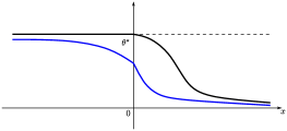
(b) $K_{1}=\theta^{*}$

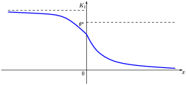
(c) $K_{1}>\theta^{*}$

Figure 3: Profile of a steady solution $U$ with $U(-\infty)\!=\!K_{1}$ and $U(+\infty)\!=\!0$, if $\int_{0}^{K_{2}}f_{2}(s)\mathrm{d}s\!>\!0$.

Now suppose that $U^{\prime}$ has a strict constant sign in $[0^{+},+\infty)$, which implies necessarily $U^{\prime}<0$ in $[0^{+},+\infty)$ since $U(0)>0$ and $U(+\infty)=0$. Then, $U^{\prime}<0$ in $(-\infty,0^{-}]$, $U(0)<K_{1}$ and (2.8) holds as before, while the inequality $U(0)<\theta^{*}$ holds too from (4.9) since $U(0)\leq\theta^{*}$ and $U^{\prime}(0^{+})<0$ (see the blue curves in Fig. 3). The proof of Proposition 2.8 is complete. ∎

Proof of Proposition 2.9.

We first claim that the existence of a positive classical stationary solution $U$ of (1.1) such that $U(-\infty)=K_{1}$ and $U(+\infty)=0$ is equivalent to the existence of $\xi>0$ such that

$$\int^{\xi}_{0}f_{2}(s)\mathrm{d}s\leq 0,~{}~{}\int^{K_{1}}_{\xi}\!f_{1}(s)\mathrm{d}s=-\frac{d_{1}\sigma^{2}}{d_{2}}\int^{\xi}_{0}f_{2}(s)\mathrm{d}s$$ (4.11)

and

$$\begin{cases}0<\xi<K_{1}~{}~{}&\displaystyle\text{if}~{}\int_{0}^{K_{2}}f_{2}(s)\mathrm{d}s<0,\cr 0<\xi<\min(K_{1},K_{2})~{}~{}&\displaystyle\text{if}~{}\int_{0}^{K_{2}}f_{2}(s)\mathrm{d}s=0,\cr 0<\xi\leq\theta^{*}~{}~{}&\displaystyle\text{if}~{}\int_{0}^{K_{2}}f_{2}(s)\mathrm{d}s>0,\end{cases}$$ (4.12)

where $\theta^{*}\in(\theta,K_{2})$ is such that $\int_{0}^{\theta^{*}}\!f_{2}(s)\mathrm{d}s=0$ when $\int_{0}^{K_{2}}\!f_{2}(s)\mathrm{d}s>0$. Assume this claim for the moment. Under the assumptions of Proposition 2.9, it is straightforward to see that such a $\xi>0$ satisfying (4.11)–(4.12) exists by qualitative comparisons of the graphs of the integrals in (4.11), namely:

• in the case $\int_{0}^{K_{2}}f_{2}(s)\mathrm{d}s<0$, since the function $\nu\mapsto\int_{\nu}^{K_{1}}f_{1}(s)\mathrm{d}s$ is continuous decreasing in $[0,K_{1}]$ and vanishes at $K_{1}$, whereas the function $\nu\mapsto-(d_{1}\sigma^{2}/d_{2})\int_{0}^{\nu}f_{2}(s)\mathrm{d}s$ is continuous in $[0,K_{1}]$, positive in $(0,K_{1}]$ and vanishes at $0$, it follows that there is $\xi\in(0,K_{1})$ satisfying (4.11);

• in the case $\int_{0}^{K_{2}}f_{2}(s)\mathrm{d}s=0$ with $K_{1}<K_{2}$, since the function $\nu\mapsto\int_{\nu}^{K_{1}}f_{1}(s)\mathrm{d}s$ is continuous decreasing in $[0,K_{1}]$ and vanishes at $K_{1}$, whereas the function $\nu\mapsto-(d_{1}\sigma^{2}/d_{2})\int_{0}^{\nu}f_{2}(s)\mathrm{d}s$ is continuous and positive in $(0,K_{2})\supseteq(0,K_{1}]$ and vanishes at $0$, then there is $\xi\in(0,K_{1})$ such that (4.11) holds true;

• in the case $\int_{0}^{K_{2}}f_{2}(s)\mathrm{d}s>0$ with $K_{1}\leq\theta^{*}$, we consider two subcases. Assume first that $K_{1}<\theta^{*}$. Since the function $\nu\mapsto\int_{\nu}^{K_{1}}f_{1}(s)\mathrm{d}s$ is continuous decreasing in $[0,K_{1}]$ and vanishes at $K_{1}$, whereas the function $\nu\mapsto-(d_{1}\sigma^{2}/d_{2})\int_{0}^{\nu}f_{2}(s)\mathrm{d}s$ is continuous and positive in $(0,\theta^{*})\supseteq(0,K_{1}]$ and vanishes at $0$, there exists $\xi\in(0,K_{1})$ such that (4.11) holds. Lastly, if $K_{1}=\theta^{*}$, then $\xi=K_{1}=\theta^{*}$ satisfies (4.11).

The conclusion of Proposition 2.9 will therefore be achieved once the claim is proved. For the proof of the claim, observe first that, if $U$ is a positive classical stationary solution of (1.1) such that $U(-\infty)=K_{1}$ and $U(+\infty)=0$, then the quantity $\xi:=U(0)>0$ necessarily satisfies (4.11)–(4.12) by Proposition 2.8. Therefore, we only have to show that the conditions (4.11)–(4.12) yield the existence of such a solution $U$. So let $\xi>0$ satisfy (4.11)–(4.12). We wish to show that (1.1) admits a positive classical stationary solution $U$ such that $U(-\infty)=K_{1}$ and $U(+\infty)=0$. Set

$$\left\{\begin{array}[]{rcl}U(0)&=&\xi,\vspace{3pt}\\ U^{\prime}(0^{+})&=&\displaystyle\text{sgn}(U(0)-K_{1})\sqrt{-\frac{2}{d_{2}}\int^{U(0)}_{0}f_{2}(s)\mathrm{d}s},\vspace{3pt}\\ U^{\prime}(0^{-})&=&\displaystyle\text{sgn}(U(0)-K_{1})\sqrt{\frac{2}{d_{1}}\int^{K_{1}}_{U(0)}f_{1}(s)\mathrm{d}s},\end{array}\right.$$ (4.13)

where sgn$(t)=t/|t|$ if $t\in\mathbb{R}^{*}$ and sgn$(0)=0$. Observe that $U^{\prime}(0^{-})=\sigma U^{\prime}(0^{+})$, thanks to (4.11) and (4.13). Given these values at $0^{\pm}$, we will now solve the two Cauchy problems in $(-\infty,0]$ and $[0,+\infty)$ and show that these two solutions, glued together, give rise to a solution $U$ of (1.1) such that $U(-\infty)=K_{1}$ and $U(+\infty)=0$.

Step 1. Consider first the Cauchy problem in $(-\infty,0]$:

$$\begin{cases}\ d_{1}U^{\prime\prime}+f_{1}(U)=0,~{}~{}x\leq 0,\cr\ U(0)=\xi>0,~{}\displaystyle U^{\prime}(0^{-})=\text{sgn}(U(0)-K_{1})\sqrt{\frac{2}{d_{1}}\int^{K_{1}}_{U(0)}f_{1}(s)\mathrm{d}s}.\end{cases}$$ (4.14)

By the Cauchy-Lipschitz theorem, (4.14) has a unique solution $U$ of class $C^{2}$ and defined in a maximal interval $(\overline{x},0]$ for some $\overline{x}\in[-\infty,0)$. Multiplying the equation in (4.14) by $U^{\prime}$ and then integrating over $[x,0]$ for any $x\in(\overline{x},0]$, and using the definition of $U^{\prime}(0^{-})$, yields

$$\frac{d_{1}}{2}(U^{\prime}(x^{-}))^{2}=\int^{K_{1}}_{U(x)}f_{1}(s)\mathrm{d}s~{}~{}\text{for all }x\in(\overline{x},0].$$ (4.15)

We claim that

$$\begin{cases}\text{ either}&\!\!U>K_{1}\hbox{ in $(\overline{x},0]$ and }U^{\prime}>0~{}\text{in}~{}(\overline{x},0^{-}],\cr\text{ or}&\!\!U<K_{1}\hbox{ in $(\overline{x},0]$ and }U^{\prime}<0~{}\text{in}~{}(\overline{x},0^{-}],\cr\text{ or}&\!\!U\equiv K_{1}\text{ in}~{}(\overline{x},0].\cr\end{cases}$$ (4.16)

For this purpose, we first prove that either $U-K_{1}$ has a strict constant sign in $(\overline{x},0]$ or $U\equiv K_{1}$ in $(\overline{x},0]$. Indeed, assume that there is $x_{0}\in(\overline{x},0]$ such that $U(x_{0})=K_{1}$, then (4.15) implies $U^{\prime}(x_{0}^{-})=0$, hence $U\equiv K_{1}$ in $(\overline{x},0]$ by the Cauchy-Lipschitz theorem. Assume now that $U-K_{1}$ has a strict constant sign in $(\overline{x},0]$. Then (4.15) implies that $U^{\prime}$ has a strict constant sign in $(\overline{x},0^{-}]$. Together with the definition of $U^{\prime}(0^{-})$ in (4.14), one concludes that, if $U(0)>K_{1}$ (respectively $U(0)<K_{1}$), then $U>K_{1}$ in $(\overline{x},0]$ and $U^{\prime}>0$ in $(\overline{x},0^{-}]$ (respectively $U<K_{1}$ in $(\overline{x},0]$ and $U^{\prime}<0$ in $(\overline{x},0^{-}]$). Our claim (4.16) is achieved.

From the above observation, we derive that $U$ is monotone and bounded in $(\overline{x},0]$ and, from the Cauchy-Lipschitz theorem, that the solution $U$ of (4.14) is defined on $(-\infty,0]$, i.e. $\overline{x}=-\infty$. Let us finally show that $U(-\infty)=K_{1}$. Let $a:=U(-\infty)$. Then, by (4.16), $a=K_{1}$ if $U(0)=K_{1}$, $K_{1}\leq a<U(0)$ if $U(0)>K_{1}$, or $U(0)<a\leq K_{1}$ if $0<U(0)<K_{1}$. Using (4.15), one has

$$\frac{d_{1}}{2}(U^{\prime}(x))^{2}\to\int^{K_{1}}_{a}\!\!f_{1}(s)\mathrm{d}s~{}~{}~{}\text{as}~{}x\to-\infty,$$

whence $U^{\prime}(-\infty)=0$ and $U(-\infty)=a=K_{1}$, from the assumption (2.4) on $f_{1}$.

Step 2. Consider now the Cauchy problem in $[0,+\infty)$:

$$\begin{cases}d_{2}U^{\prime\prime}+f_{2}(U)=0,~{}~{}x\geq 0,\cr\displaystyle U(0)=\xi>0,~{}U^{\prime}(0^{+})=\text{sgn}(U(0)-K_{1})\sqrt{-\frac{2}{d_{2}}\int^{U(0)}_{0}\!\!f_{2}(s)\mathrm{d}s}.\end{cases}$$ (4.17)

The solution of (4.17) exists, is of class $C^{2}$ and is unique in a maximal interval $[0,x^{*})$, for some ${x^{*}}\in(0,+\infty]$. Integrating the equation in (4.17) against $U^{\prime}$ over $[0,x]$ for any $x\in[0,{x^{*}})$, and using the expression of $U^{\prime}(0^{+})$, yields

$$\frac{d_{2}}{2}(U^{\prime}(x^{+}))^{2}=\left\{\begin{array}[]{lll}\displaystyle-\int_{0}^{U(x)}f_{2}(s)\mathrm{d}s&\hbox{for all $x\in[0,{x^{*}})$}&\hbox{if $U(0)\neq K_{1}$},\vspace{3pt}\\ \displaystyle-\int_{U(0)}^{U(x)}f_{2}(s)\mathrm{d}s&\hbox{for all $x\in[0,{x^{*}})$}&\hbox{if $U(0)=K_{1}$}.\end{array}\right.$$ (4.18)

Notice from (4.12)–(4.13) that the case $U(0)=K_{1}$ can only occur when $\int_{0}^{K_{2}}f_{2}(s)\mathrm{d}s>0$, and then $\xi=U(0)=K_{1}=\theta^{*}$ by (4.11), while $U^{\prime}(0^{+})=0$ by (4.13). In that case, by uniqueness, $U$ is equal in $[0,+\infty)$ to the half-bump associated to the reaction $f_{2}$, that is, $x^{*}=+\infty$, $U^{\prime}<0$ in $(0,+\infty)$, $U(+\infty)=0$, $U(0)=\theta^{*}$ and $U^{\prime}(0^{+})=0$.

Therefore, one can assume in the sequel that $U(0)\neq K_{1}$. We observe that $U>0$ in $[0,{x^{*}})$. Indeed, otherwise, there is $x_{0}\in(0,{x^{*}})$ such that $U(x_{0})=0$, hence $U^{\prime}(x_{0})=0$ by (4.18) and $U\equiv 0$ in $[0,x^{*})$ by the Cauchy-Lipschitz theorem. This would contradict $U(0)>0$. Thus, $U>0$ in $[0,{x^{*}})$. Next, we solve (4.17) by dividing into three cases according to the sign of the mass $\int_{0}^{K_{2}}f_{2}(s)\mathrm{d}s$.

Case 1: $\int_{0}^{K_{2}}f_{2}(s)\mathrm{d}s<0$. One infers from (4.12) that $U(0)=\xi<K_{1}$ and thus $U^{\prime}(0^{+})<0$ by (4.17). Moreover, one deduces from (4.18) that $U^{\prime}$ does not change sign in $[0^{+},{x^{*}})$. Therefore, $U^{\prime}<0$ in $[0^{+},{x^{*}})$. Since $U>0$ in $[0,{x^{*}})$, one has $0<U<U(0)<K_{1}$ in $(0,{x^{*}})$, whence ${x^{*}}=+\infty$. Define $b:=U(+\infty)\geq 0$. From (4.18), it follows that

$$\frac{d_{2}}{2}(U^{\prime}(x))^{2}\to-\int_{0}^{b}f_{2}(s)\mathrm{d}s~{}~{}~{}\text{as}~{}x\to+\infty,$$

hence, $U^{\prime}(+\infty)=0$ and $U(+\infty)=b=0$.

Case 2: $\int_{0}^{K_{2}}f_{2}(s)\mathrm{d}s=0$. It follows from (4.12) that $0<U(0)=\xi<\min(K_{1},K_{2})$ and thus $U^{\prime}(0^{+})<0$ by (4.17). We now show that $U^{\prime}<0$ in $(0,{x^{*}})$. Assume by contradiction that there is $x_{0}=\min\{x\in(0,{x^{*}}):U^{\prime}(x)=0\}\ \in(0,x^{*})$. Then $0<U(x_{0})<U<U(0)<\min(K_{1},K_{2})$ in $(0,x_{0})$. On the other hand, taking $x=x_{0}$ in (4.18) and using $U(x_{0})>0$ yields $U(x_{0})=K_{2}$, a contradiction. Thus, $U^{\prime}<0$ in $[0^{+},{x^{*}})$, whence $0<U<U(0)$ in $(0,{x^{*}})$ and ${x^{*}}=+\infty$. As in Case 1, one concludes that $U(+\infty)=0$.

Case 3: $\int_{0}^{K_{2}}f_{2}(s)\mathrm{d}s>0$. We let $\theta^{*}\in(\theta,K_{2})$ be such that $\int_{0}^{\theta^{*}}\!f_{2}(s)\mathrm{d}s=0$ and $Q\in(\theta^{*},+\infty]$ be as in (4.10). From (4.12), it is seen that $0<U(0)=\xi\leq\theta^{*}$. Moreover, we observe from (4.18) that $U(x)\notin(\theta^{*},Q)$ for every $x\in[0,{x^{*}})$, hence $0<U\leq\theta^{*}$ in $[0,x^{*})$ and $x^{*}=+\infty$. We recall that the bistable equation $d_{2}u^{\prime\prime}+f_{2}(u)=0$ in $\mathbb{R}$ admits an even bump-like solution $u$, satisfying

$$u(0)=\theta^{*},~{}u^{\prime}(0)=0,~{}u^{\prime}<0~{}\text{in}~{}(0,+\infty),~{}u(\pm\infty)=0.$$

1. Suppose first that $K_{1}<U(0)=\xi\ (\leq\theta^{*})$, whence $U^{\prime}(0^{+})>0$ and $K_{1}<U(0)=\xi<\theta^{*}$ by (4.11) and (4.17). If $U^{\prime}>0$ in $[0^{+},+\infty)$, then $U(+\infty)$ exists and belongs to $(0,\theta^{*}]$, and $U^{\prime}(+\infty)=U^{\prime\prime}(+\infty)=0$ from standard elliptic estimates. Together with (4.18), one gets that $U(+\infty)=\theta^{*}$, hence $U^{\prime\prime}(x)=-f_{2}(U(x))/d_{2}\to-f_{2}(\theta^{*})/d_{2}<0$ as $x\to+\infty$, a contradiction. Therefore, $U$ has a critical point in $(0,+\infty)$, that is, $x_{0}=\min\{x>0:U^{\prime}(x)=0\}$ is a well defined positive real number, and one has $U^{\prime}>0$ in $(0,x_{0})$ and $U^{\prime}(x_{0})=0$. Combining (4.18) with the fact that $0<U\leq\theta^{*}$ in $[0,+\infty)$, one infers that $U(x_{0})=\theta^{*}$. Therefore, by the uniqueness of the solution to the Cauchy problem, $U$ has to be the bump-like solution $u(\cdot-x_{0})$ in $[0,+\infty)$. Namely, $U(x_{0})=\theta^{*}$, $U^{\prime}(x_{0})=0$, $U^{\prime}<0$ in $(x_{0},+\infty)$ and $U(+\infty)=0$.

2. Finally, let us assume $U(0)=\xi<K_{1}$. Then, $U^{\prime}(0^{+})<0$ by (4.11) and (4.17). Remember also that $0<U(0)=\xi\leq\theta^{*}$. We now show that $U^{\prime}<0$ in $(0,+\infty)$. If not, then there is $x_{0}=\min\{x>0:U^{\prime}(x)=0\}>0$ such that $U^{\prime}(x_{0})=0$ and $0<U(x_{0})<U<U(0)\leq\theta^{*}$ in $(0,x_{0})$. It follows from (4.18) that $0=(d_{2}/2)(U^{\prime}(x_{0}))^{2}=-\int_{0}^{U(x_{0})}f_{2}(s)\mathrm{d}s>0$, a contradiction. Consequently, $U^{\prime}<0$ in $(0,+\infty)$ and the argument used in Case 1 yields $U(+\infty)=0$.

Gluing the solutions of (4.14) and (4.17) proves the existence of the desired stationary solution $U$ of (1.1) such that $U(-\infty)=K_{1}$ and $U(+\infty)=0$. Therefore, our claim at the beginning of the proof is achieved and the proof of Proposition 2.9 is thereby complete. ∎

Remark 4.1.

Based on the above proof, it is easy to find examples of functions $f_{1,2}$ satisfying (2.4)–(2.5) and $\int_{0}^{K_{2}}f_{2}(s)\mathrm{d}s>0$ such that (1.1) has no stationary solution $U$ connecting $K_{1}$ and $0$. For instance, let us take $d_{1}=d_{2}=\sigma=1$, and set

$$f_{1}(u)=u(K_{1}-u),~{}~{}f_{2}(u)=u(K_{2}-u)(u-\theta)$$

with $K_{1}=K_{2}=4$ and $\theta=1$. It is straightforward to check that (4.11) $($with $\xi>0$$)$ yields $\xi>4$, contradicting the condition $\xi\leq\theta^{*}<4$ implied by (4.12). Therefore, (4.11) and (4.12) can not be fulfilled simultaneously, and there is no positive classical stationary solution $U$ of (1.1) such that $U(-\infty)=K_{1}$ and $U(+\infty)=0$.

Proof of Proposition 2.10.

The strategy is very similar to that of Proposition 2.9. For completeness, we sketch the proof. Here, in addition to (2.4)–(2.5), we assume that $\int_{0}^{K_{2}}f_{2}(s)\mathrm{d}s\geq 0$. We first claim that the existence (respectively the existence and uniqueness) of a positive classical stationary solution $V$ of (1.1) satisfying $V(-\infty)=K_{1}$ and $V(+\infty)=K_{2}$ is equivalent to the existence (respectively the existence and uniqueness) of $\xi>0$ such that

$$\begin{cases}\ \xi=K_{1}=K_{2}&\text{if}~{}K_{1}=K_{2},\cr\ \min(K_{1},K_{2})<\xi<\max(K_{1},K_{2})&\text{if}~{}K_{1}\neq K_{2},\end{cases}$$ (4.19)

and

$$\int_{\xi}^{K_{1}}\!f_{1}(s)\mathrm{d}s=\frac{d_{1}\sigma^{2}}{d_{2}}\int_{\xi}^{K_{2}}\!f_{2}(s)\mathrm{d}s.$$ (4.20)

In this paragraph, we observe that such $\xi>0$ satisfying (4.19)–(4.20) always exists, and is unique if $K_{1}\geq\theta$. To check this, it is sufficient to consider the case of $K_{1}\neq K_{2}$. Suppose $K_{1}<K_{2}$. Observe that the function $\nu\mapsto\int_{\nu}^{K_{1}}f_{1}(s)\mathrm{d}s$ is continuous increasing in $[K_{1},K_{2}]$ and vanishes at $K_{1}$, whereas the function $\nu\mapsto(d_{1}\sigma^{2}/d_{2})\int_{\nu}^{K_{2}}f_{2}(s)\mathrm{d}s$ is continuous positive in $[K_{1},K_{2})$, vanishes at $K_{2}$, and is either increasing in $[K_{1},\theta]$ and decreasing in $[\theta,K_{2}]$ (if $K_{1}<\theta$), or decreasing in $[K_{1},K_{2}]$ (if $K_{1}\geq\theta$). Therefore, there is $\xi\in(K_{1},K_{2})$ such that (4.20) is satisfied, and $\xi$ is unique if $K_{1}\geq\theta$. Consider now the case of $K_{2}<K_{1}$. Since the function $\nu\mapsto\int_{\nu}^{K_{1}}f_{1}(s)\mathrm{d}s$ is continuous decreasing in $[K_{2},K_{1}]$ and vanishes at $K_{1}$, whereas the function $\nu\mapsto(d_{1}\sigma^{2}/d_{2})\int_{\nu}^{K_{2}}f_{2}(s)\mathrm{d}s$ is continuous increasing in $[K_{2},K_{1}]$ and vanishes at $K_{2}$, it follows that there is a unique $\xi\in(K_{2},K_{1})$ satisfying (4.20).

Therefore, it remains to prove our claim, whose proof is divided into two steps, each corresponding to one implication of the equivalence.

Step 1: necessary condition for the existence of $V$. Suppose $V$ is a positive classical stationary solution of (1.1) satisfying $V(-\infty)=K_{1}$ and $V(+\infty)=K_{2}$. Multiplying $d_{1}V^{\prime\prime}+f_{1}(V)=0$ by $V^{\prime}$ and integrating the resulting equation over $(-\infty,x]$ for any $x\in(-\infty,0]$ yields

$$\frac{d_{1}}{2}(V^{\prime}(x^{-}))^{2}=\int_{V(x)}^{K_{1}}f_{1}(s)\mathrm{d}s\ \hbox{ for all }x\leq 0.$$ (4.21)

Similarly, one also derives that

$$\frac{d_{2}}{2}(V^{\prime}(x^{+}))^{2}=\int^{K_{2}}_{V(x)}f_{2}(s)\mathrm{d}s\geq 0\ \hbox{ for all }x\geq 0.$$ (4.22)

Following the same argument as for (4.15)-(4.16), one derives from (4.21) that $V$ is monotone in patch $1$ and, more precisely,

$$\begin{cases}\text{ either}&\!\!V>K_{1}\hbox{ in $(-\infty,0]$ and }V^{\prime}>0~{}\text{in}~{}(-\infty,0^{-}],\cr\text{ or}&\!\!V<K_{1}\hbox{ in $(-\infty,0]$ and }V^{\prime}<0~{}\text{in}~{}(-\infty,0^{-}],\cr\text{ or}&\!\!V\equiv K_{1}~{}\text{in}~{}(-\infty,0].\cr\end{cases}$$

Similarly, since $\int_{\nu}^{K_{2}}f_{2}(s)\mathrm{d}s>0$ for all $\nu\in(0,K_{2})\cup(K_{2},+\infty)$, it follows from (4.22) that $V$ is also monotone in patch 2 and, more precisely,

$$\begin{cases}\text{ either}&\!\!V>K_{2}\hbox{ in $[0,+\infty)$ and }\ V^{\prime}<0~{}\text{in}~{}[0^{+},+\infty),\cr\text{ or}&\!\!V<K_{2}\hbox{ in $[0,+\infty)$ and }\ V^{\prime}>0~{}\text{in}~{}[0^{+},+\infty),\cr\text{ or}&\!\!V\equiv K_{2}~{}\text{in}~{}[0,+\infty).\cr\end{cases}$$

Using $V^{\prime}(0^{-})=\sigma V^{\prime}(0^{+})$, one then infers that $V$ is monotone in $\mathbb{R}$ and, more precisely,

$$\begin{cases}\ V\equiv K_{1}=K_{2}~{}~{}&\text{if}~{}~{}K_{1}=K_{2},\cr\ \min(K_{1},K_{2})<V<\max(K_{1},K_{2})\text{ and sgn}(V^{\prime})=\text{sgn}(V(0)-K_{1})~{}~{}&\text{if}~{}~{}K_{1}\neq K_{2}.\end{cases}$$

Moreover, thanks to (4.21)–(4.22), $V(0)$ satisfies

$$\int_{V(0)}^{K_{1}}f_{1}(s)\mathrm{d}s=\frac{d_{1}\sigma^{2}}{d_{2}}\int_{V(0)}^{K_{2}}f_{2}(s)\mathrm{d}s.$$

Hence, the quantity $\xi=V(0)$ satisfies (4.19)–(4.20).

Step 2: sufficient condition for the existence of $V$. Assume that there is $\xi>0$ satisfying (4.19)–(4.20). If $K_{1}=K_{2}$, then $\xi=K_{1}=K_{2}$ and the function $V\equiv K_{1}=K_{2}$ obviously satisfies (1.1) with $V(-\infty)=K_{1}=K_{2}=V(+\infty)$. One can then assume in the sequel that $K_{1}\neq K_{2}$. Let us set $V(0)=\xi\in(\min(K_{1},K_{2}),\max(K_{1},K_{2}))$ and define

$$V^{\prime}(0^{-})=\text{sgn}(V(0)-K_{1})\sqrt{\frac{2}{d_{1}}\int^{K_{1}}_{V(0)}f_{1}(s)\mathrm{d}s},$$

and

$$V^{\prime}(0^{+})=\text{sgn}(V(0)-K_{1})\sqrt{\frac{2}{d_{2}}\int_{V(0)}^{K_{2}}f_{2}(s)\mathrm{d}s}.$$

It is obvious to see that $V^{\prime}(0^{-})=\sigma V^{\prime}(0^{+})$, thanks to (4.20). Notice also that $V(0)=\xi\neq K_{1}$, here.

Step 2.1. As for (4.14), the solution $V$ of the Cauchy problem

$$\begin{cases}\ d_{1}V^{\prime\prime}+f_{1}(V)=0,~{}~{}x\leq 0,\cr\ V(0)=\xi>0,~{}\displaystyle V^{\prime}(0^{-})=\text{sgn}(V(0)-K_{1})\sqrt{\frac{2}{d_{1}}\int^{K_{1}}_{V(0)}f_{1}(s)\mathrm{d}s}.\end{cases}$$ (4.23)

is defined in $(-\infty,0]$ and satisfies (4.16) with $V$ instead of $U$ and $\overline{x}=-\infty$, that is,

$$\begin{cases}\text{ either}&\!\!\!V>K_{1}\hbox{ in $(-\infty,0]$ and }V^{\prime}>0~{}\text{in}~{}(-\infty,0^{-}],\cr\text{ or}&\!\!\!V<K_{1}\hbox{ in $(-\infty,0]$ and }V^{\prime}<0~{}\text{in}~{}(-\infty,0^{-}],\cr\end{cases}$$

and $V(-\infty)=K_{1}$.

Step 2.2. Let $V$ denote the solution of

$$\begin{cases}d_{2}V^{\prime\prime}+f_{2}(V)=0,~{}~{}x\geq 0,\cr V(0)=\xi>0,~{}\displaystyle V^{\prime}(0^{+})=\text{sgn}(V(0)-K_{1})\sqrt{\frac{2}{d_{2}}\int_{V(0)}^{K_{2}}f_{2}(s)\mathrm{d}s}.\end{cases}$$ (4.24)

Notice that, here, $\min(K_{1},K_{2})<V(0)<\max(K_{1},K_{2})$, hence $V^{\prime}(0^{+})\neq 0$ since $\int_{\nu}^{K_{2}}f_{2}(s)\mathrm{d}s>0$ for all $\nu\in\mathbb{R}\setminus\{0,K_{2}\}$. The Cauchy-Lipschitz theorem implies that there is a unique solution of (4.24) defined in a maximal interval $[0,x^{*})$ for some $x^{*}\in(0,+\infty]$. Multiplying the equation in (4.24) by $V^{\prime}$ and then integrating over $[0,x]$ for any $x\in[0,x^{*})$, and using the formula of $V^{\prime}(0^{+})$, yields

$$\frac{d_{2}}{2}(V^{\prime}(x^{+}))^{2}=\int^{K_{2}}_{V(x)}f_{2}(s)\mathrm{d}s\ \hbox{ for all }x\in[0,x^{*}).$$ (4.25)

Moreover, we claim that $V^{\prime}$ has a strict constant sign in $[0^{+},x^{*})$. Indeed, otherwise, there is $x_{0}\in[0^{+},x^{*})$ such that $V^{\prime}(x_{0})=0$, and (4.25) implies that

$$\begin{cases}\ V(x_{0})=K_{2}~{}~{}&\displaystyle\text{if}~{}~{}\int_{0}^{K_{2}}f_{2}(s)\mathrm{d}s>0,\cr\ V(x_{0})=K_{2}~{}\text{or}~{}0~{}~{}&\displaystyle\text{if}~{}~{}\int_{0}^{K_{2}}f_{2}(s)\mathrm{d}s=0.\end{cases}$$

Thus, one would derive $V\equiv K_{2}$ or $V\equiv 0$ in $[0,x^{*})$ by the Cauchy-Lipschitz theorem, contradicting $\min(K_{1},K_{2})<V(0)=\xi<\max(K_{1},K_{2})$. Thus, $V^{\prime}$ has a constant strict sign in $[0^{+},x^{*})$. Hence, $V(x)\neq K_{2}$ for every $x\in[0,x^{*})$, by (4.25). Therefore, we conclude that

$$\begin{cases}\text{ if}~{}K_{1}<V(0)<K_{2},\hbox{ then }V^{\prime}>0~{}\text{in}~{}[0^{+},x^{*})\hbox{ and }K_{1}<V<K_{2}~{}\text{in}~{}[0,x^{*}),\cr\text{ if}~{}K_{2}<V(0)<K_{1},\hbox{ then }V^{\prime}<0~{}\text{in}~{}[0^{+},x^{*})\hbox{ and }K_{2}<V<K_{1}~{}\text{in}~{}[0,x^{*}).\end{cases}$$

Both cases imply that $x^{*}=+\infty$. Defining $V(+\infty)=a$, one has $K_{1}\leq a\leq K_{2}$ and (4.25) implies

$$\frac{d_{2}}{2}(V^{\prime}(x))^{2}\to\int^{K_{2}}_{a}f_{2}(s)\mathrm{d}s~{}~{}~{}\text{as}~{}x\to+\infty,$$

hence $V^{\prime}(+\infty)=0$ and $V(+\infty)=a=K_{2}$.

Step 2.3: conclusion. By gluing the solutions of the above two Cauchy problems (4.23) and (4.24), one obtains the existence of a monotone positive classical stationary solution $V$ of (1.1) such that $V(-\infty)=K_{1}$ and $V(+\infty)=K_{2}$. Lastly, if $K_{1}\geq\theta$, then we have already seen that $\xi>0$ solving (4.19)–(4.20) is unique, hence the above proof shows that $V(0)=\xi$ is unique and the positive classical stationary solution $V$ of (1.1) such that $V(-\infty)=K_{1}$ and $V(+\infty)=K_{2}$ is itself unique. The proof of Proposition 2.10 is thereby complete. ∎

4.3 Blocking in the bistable patch 2: proof of Theorem 2.11

In this section, we study the qualitative behavior of the solution $u$ to (1.1) under the KPP-bistable assumptions (2.4)–(2.5). We carry out the proof of Theorem 2.11 on various sufficient conditions for blocking in the bistable patch 2. The proof is based, among other things, on a comparison with some barriers, such as a traveling front with negative or zero speed (up to some exponentially small terms, when $\int_{0}^{K_{2}}\!f_{2}(s)\mathrm{d}s\leq 0$), or a stationary solution connecting $K_{1}$ to $0$ (when $\|u_{0}\|_{L^{1}(\mathbb{R})}$ is small enough).

Proof of Theorem 2.11.

(i) We first assume that

$$\int_{0}^{K_{2}}f_{2}(s)\mathrm{d}s<0.$$

Let $u$ be the solution to the Cauchy problem (1.1) with a nonnegative continuous and compactly supported initial datum $u_{0}\not\equiv 0$. The strategy of the proof consists in constructing a supersolution which blocks the solution $u(t,x)$ for all times $t\geq 0$ as $x\to+\infty$. Set $M:=\max\big{(}K_{1},K_{2},\|u_{0}\|_{L^{\infty}(\mathbb{R})}\big{)}+1$. Since the function $f_{2}$ satisfies (2.5) with $\int_{0}^{K_{2}}f_{2}(s)\mathrm{d}s<0$, there is a $C^{1}(\mathbb{R})$ function $\overline{f}_{2}$ such that $\overline{f}_{2}\geq f_{2}$ in $\mathbb{R}$, $\overline{f}_{2}(0)=\overline{f}_{2}(\theta)=\overline{f}_{2}(M)=0$, $\overline{f}_{2}^{\prime}(0)<0$, $\overline{f}_{2}^{\prime}(M)<0$, $\overline{f}_{2}>0$ in $(-\infty,0)\cup(\theta,M)$, $\overline{f}_{2}<0$ in $(0,\theta)\cup(M,+\infty)$, and $\int_{0}^{M}\overline{f}_{2}(s)\mathrm{d}s<0$ (it is even possible to choose $\overline{f}_{2}$ so that $\overline{f}_{2}=f_{2}$ in $(-\infty,K_{2}-\delta]$ for some small $\delta>0$). There is then a decreasing front profile $\overline{\phi}$ solving (2.6) with $\overline{f}_{2}$ and $M$ instead of $f_{2}$ and $K_{2}$, and with negative speed $\overline{c}_{2}$ instead of $c_{2}$. Since $\overline{\phi}(-\infty)=M>\max(K_{1},\|u_{0}\|_{L^{\infty}(\mathbb{R})})$ and $u_{0}$ is compactly supported, one can then choose $A>0$ large enough so that $u_{0}(x)\leq\overline{\phi}(x-A)$ for all $x\geq 0$, $u_{0}(x)\leq\overline{\phi}(-A)$ for all $x\leq 0$, and $K_{1}\leq\overline{\phi}(-A)$. Set, for $(t,x)\in[0,+\infty)\times\mathbb{R}$,

$$\overline{u}(t,x)=\left\{\begin{array}[]{ll}\overline{\phi}(x-A)&\hbox{if }x\geq 0,\vspace{3pt}\\ \overline{\phi}(-A)&\hbox{if }x<0.\end{array}\right.$$

Since $f_{1}(\overline{\phi}(-A))\leq 0$ by (2.4), since $d_{2}\overline{\phi}^{\prime\prime}+f_{2}(\overline{\phi})\leq d_{2}\overline{\phi}^{\prime\prime}+\overline{f}_{2}(\overline{\phi})=-\overline{c}_{2}\overline{\phi}^{\prime}<0$ in $\mathbb{R}$ and since $\overline{\phi}^{\prime}(-A)<0$, it follows that $\overline{u}$ is a supersolution of (1.1) in the sense of Definition 2.2, while $u_{0}\leq\overline{u}(0,\cdot)$ in $\mathbb{R}$. Therefore, Proposition 2.4 implies that $u(t,x)\leq\overline{u}(t,x)$ for all $(t,x)\in[0,+\infty)\times\mathbb{R}$. Since $u$ is nonnegative and $\overline{\phi}(+\infty)=0$, this immediately yields the blocking property (2.9).

(ii) We then assume that $\int_{0}^{K_{2}}f_{2}(s)\mathrm{d}s=0$ and $K_{1}<K_{2}$. First, it is convenient to introduce some parameters. Let $\varepsilon>0$ be such that

$$0<\varepsilon<\min\left(\frac{|f_{2}^{\prime}(0)|}{2},\frac{|f_{2}^{\prime}(K_{2})|}{2}\right),\ \ f_{2}^{\prime}\leq\frac{f_{2}^{\prime}(0)}{2}~{}\text{in}~{}[0,2\varepsilon],~{}~{}f_{2}^{\prime}\leq\frac{f_{2}^{\prime}(K_{2})}{2}~{}\text{in}~{}[K_{2}-\varepsilon,K_{2}+\varepsilon].$$ (4.26)

Choose $C>0$ large enough such that

$$\phi\geq K_{2}-\varepsilon~{}\text{in}~{}(-\infty,-C]\ \hbox{ and }\ \phi\leq\varepsilon~{}\text{in}~{}[C,+\infty).$$ (4.27)

As the front profile $\phi$ solving (2.6) is such that $\phi^{\prime}$ is negative and continuous, there is $\kappa>0$ such that

$$-\phi^{\prime}\geq\kappa>0~{}~{}\text{in}~{}[-C,C].$$ (4.28)

Finally, pick $\rho>0$ be such that

$$\kappa\rho\geq\varepsilon+\max_{[0,K_{2}+\varepsilon]}|f_{2}^{\prime}|.$$ (4.29)

Let $u$ be the solution to the Cauchy problem (1.1) with a nonnegative continuous and compactly supported initial datum $u_{0}\not\equiv 0$ and let $V$ be a positive monotone classical stationary solution of (1.1) such that $V(-\infty)=K_{1}$ and $V(+\infty)=K_{2}$, given in Proposition 2.10. Denote $w$ the solution to (1.1) with initial datum $w(0,\cdot)=M:=\max\big{(}K_{2},\|u_{0}\|_{L^{\infty}(\mathbb{R})}\big{)}$. As in the proof of the first part of Theorem 2.6, Proposition 2.4 implies that $w$ is nonincreasing in time, and that $0<u(t,x)<w(t,x)\leq M$ and $V(x)<w(t,x)$ for all $t>0$ and $x\in\mathbb{R}$. From the Schauder estimates of Proposition 2.3, it follows that $w(t,x)$ converges as $t\to+\infty$, locally uniformly in $x\in\mathbb{R}$, to a stationary solution $q$ of (1.1), such that $M\geq q(x)\geq V(x)\geq K_{1}$ for all $x\in\mathbb{R}$ and

$$\limsup_{t\to+\infty}u(t,\cdot)\leq q~{}~{}\text{locally uniformly in}~{}\mathbb{R}.$$ (4.30)

As shown in Theorem 2.7, one also has $q(-\infty)=K_{1}$. On the other hand, since $f_{2}<0$ in $(K_{2},+\infty)$ and $q$ is bounded, one easily infers that $\limsup_{x\to+\infty}q(x)\leq K_{2}$. Furthermore, as in the proof of Propositions 2.5 and 2.8, the function $q$ is monotone in $(-\infty,0]$, and $q^{\prime}$ has a constant strict sign in $(-\infty,0^{-}]$ unless $q\equiv K_{1}$ in $(-\infty,0]$. Thus, if one would assume that $\sup_{\mathbb{R}}q>K_{2}\,(>K_{1})$, there would exist $x_{0}\in(0,+\infty)$ such that $q(x_{0})=\sup_{\mathbb{R}}q>K_{2}$, which is impossible since $f_{2}<0$ in $(K_{2},+\infty)$. Therefore, $q\leq K_{2}$ in $\mathbb{R}$ and even $q<K_{2}$ in $\mathbb{R}$ since the constant $K_{2}$ is a supersolution of (1.1) and the stationary solution $q$ can not be identically equal to $K_{2}$.

Similarly, we claim that

$$\limsup_{A\to+\infty}\Big{(}\sup_{t\geq A,\,x\geq A}u(t,x)\Big{)}\leq K_{2}.$$ (4.31)

Indeed, otherwise, since $u$ is bounded in $[0,+\infty)\times\mathbb{R}$, there are $\overline{K}_{2}\in(K_{2},+\infty)$ (with $\overline{K}_{2}$ the above limsup) and two sequences $(t_{n})_{n\in\mathbb{N}}$ and $(x_{n})_{n\in\mathbb{N}}$ diverging to $+\infty$ such that $u(t_{n},x_{n})\to\overline{K}_{2}$ as $n\to+\infty$ and $\limsup_{n\to+\infty}u(t_{n}+t,x_{n}+x)\leq\overline{K}_{2}$ for all $(t,x)\in\mathbb{R}\times\mathbb{R}$. From parabolic estimates, the functions $(t,x)\mapsto u(t_{n}+t,x_{n}+x)$ converge in $C^{1;2}_{t;x;loc}(\mathbb{R}\times\mathbb{R})$, up to extraction of a subsequence, to a bounded classical solution $u_{\infty}$ of $(u_{\infty})_{t}=d_{2}(u_{\infty})_{xx}+f_{2}(u_{\infty})$ in $\mathbb{R}\times\mathbb{R}$ with $u_{\infty}\leq u_{\infty}(0,0)=\overline{K}_{2}$ in $\mathbb{R}\times\mathbb{R}$. The negativity of $f_{2}(\overline{K}_{2})$ leads to a contradiction. Therefore, (4.31) holds.

Let then $X>0$ be large enough so that

$$u(t,x)\leq K_{2}+\frac{\varepsilon}{2}\ \hbox{ for all $t\geq X$ and $x\geq X$}.$$ (4.32)

Thanks to (4.30) and $q(X)<K_{2}$, there is $T\geq X$ so large that

$$\sup_{t\geq T}\,u(t,X)<K_{2}.$$ (4.33)

Remember that the front profile $\phi$ associated with the reaction $f_{2}$, given in (2.6) with speed $c_{2}=0$ (since $\int_{0}^{K_{2}}f_{2}(s)\mathrm{d}s=0$), satisfies $\phi(-\infty)=K_{2}$. Due to (4.32)–(4.33) and the Gaussian upper bound of $u(t,x)$ for $|x|$ large at each time $t>0$ derived in Lemma A.1, together with the exponential lower bound of $\phi(s)$ as $s\to+\infty$ in (2.7), there exists $B>0$ large enough such that

$$u(T,x)\leq\phi(x-X-B-C)+\varepsilon~{}\text{for all}~{}x\geq X,\ \hbox{ and }\ \sup_{t\geq T}\,u(t,X)\leq\phi(-B-C).$$ (4.34)

Define

$$\overline{u}(t,x)=\phi(\zeta(t,x))+\varepsilon e^{-\varepsilon(t-T)}~{}~{}\text{for}~{}t\geq T~{}\text{and}~{}x\geq X,$$

where $\zeta(t,x)=x-X+\rho e^{-\varepsilon(t-T)}-\rho-B-C$. We wish to show that $\overline{u}(t,x)$ is a supersolution of the equation $u_{t}=d_{2}u_{xx}+f_{2}(u)$ for $t\geq T$ and $x\geq X$. First of all, at time $t=T$, one has

$$\overline{u}(T,x)=\phi(x-X-B-C)+\varepsilon\geq u(T,x)$$

for $x\geq X$, thanks to (4.34). Furthermore, for $t\geq T$, $\overline{u}(t,X)=\phi(\rho e^{-\varepsilon(t-T)}-\rho-B-C)+\varepsilon e^{-\varepsilon(t-T)}\geq\phi(-B-C)\geq u(t,X)$ by (4.34) again. It then remains to check that

$$\mathcal{N}\overline{u}(t,x):=\overline{u}_{t}(t,x)-d_{2}\overline{u}_{xx}(t,x)-f_{2}(\overline{u}(t,x))\geq 0$$

for $t\geq T$ and $x\geq X$. A direct computation leads to

$$\mathcal{N}\overline{u}(t,x)=f_{2}(\phi(\zeta(t,x)))-f_{2}(\overline{u}(t,x))-\phi^{\prime}(\zeta(t,x))\rho\varepsilon e^{-\varepsilon(t-T)}-\varepsilon^{2}e^{-\varepsilon(t-T)}.$$

We divide the proof into three cases:

• if $\zeta(t,x)\leq-C$, one has $K_{2}+\varepsilon\geq\overline{u}(t,x)\geq\phi(\zeta(t,x))\geq K_{2}-\varepsilon$ by (4.27); one then derives from (4.26) and the negativity of $\phi^{\prime}$ that

  $$\mathcal{N}\overline{u}(t,x)\geq-\frac{f_{2}^{\prime}(K_{2})}{2}\varepsilon e^{-\varepsilon(t-T)}-\varepsilon^{2}e^{-\varepsilon(t-T)}=\Big{(}-\frac{f_{2}^{\prime}(K_{2})}{2}-\varepsilon\Big{)}\varepsilon e^{-\varepsilon(t-T)}\geq 0;$$

• if $\zeta(t,x)\geq C$, then $0<\phi(\zeta(t,x))\leq\varepsilon$ by (4.27) and $0<\overline{u}(t,x)\leq 2\varepsilon$; it follows from (4.26) and the negativity of $\phi^{\prime}$ that

  $$\mathcal{N}\overline{u}(t,x)\geq-\frac{f_{2}^{\prime}(0)}{2}\varepsilon e^{-\varepsilon(t-T)}-\varepsilon^{2}e^{-\varepsilon(t-T)}=\Big{(}-\frac{f_{2}^{\prime}(0)}{2}-\varepsilon\Big{)}\varepsilon e^{-\varepsilon(t-T)}\geq 0;$$

• eventually, if $-C\leq\zeta(t,x)\leq C$, then $-\phi^{\prime}(\zeta(t,x))\geq\kappa>0$ by (4.28), and (4.29) then yields

$$\mathcal{N}\overline{u}(t,x)\geq-\!\max_{[0,K_{2}+\varepsilon]}\!|f_{2}^{\prime}|\,\varepsilon e^{-\varepsilon(t-T)}\!+\!\kappa\rho\varepsilon e^{-\varepsilon(t-T)}\!-\!\varepsilon^{2}e^{-\varepsilon(t-T)}\geq\Big{(}\kappa\rho-\!\max_{[0,K_{2}+\varepsilon]}\!|f_{2}^{\prime}|\!-\!\varepsilon\Big{)}\varepsilon e^{-\varepsilon(t-T)}\geq 0.$$

In conclusion, the function $\overline{u}$ is a supersolution of $u_{t}=d_{2}u_{xx}+f_{2}(u)$ for $t\geq T$ and $x\geq X$. The maximum principle implies that

$$u(t,x)\leq\overline{u}(t,x)=\phi(x-X+\rho e^{-\varepsilon(t-T)}-\rho-B-C)+\varepsilon e^{-\varepsilon(t-T)}~{}~{}\text{for all}~{}t\geq T~{}\text{and}~{}x\geq X.$$

Consequently, $\limsup_{x\to+\infty}\!\!\big{(}\sup_{t\geq T}u(t,x)\big{)}\!\leq\!\varepsilon$. On the other hand, Lemma A.1 implies that $u(t,x)\!\to\!0$ as $x\to+\infty$ locally uniformly in $t\geq 0$. Since $\varepsilon>0$ can be chosen arbitrarily small, one gets that $u$ is blocked in patch 2 and satisfies (2.9). This completes the proof of part (ii) of Theorem 2.11.

(iii) We here assume that $K_{1}<\theta$. Let $u$ be the solution to (1.1) with a nonnegative continuous and compactly supported initial datum $u_{0}\not\equiv 0$ satisfying $u_{0}<\theta$ in $\mathbb{R}$. The constant function equal to $M:=\max\big{(}K_{1},\|u_{0}\|_{L^{\infty}(\mathbb{R})}\big{)}$ is a supersolution of (1.1) in the sense of Definition 2.2 (since $f_{1}(M)\leq 0$ and $f_{2}(M)<0$), and Proposition 2.4 then implies that

$$0<u(t,x)<\max\big{(}K_{1},\|u_{0}\|_{L^{\infty}(\mathbb{R})}\big{)}<\theta\ \hbox{ for all $t\geq 0$ and $x\in\mathbb{R}$}.$$ (4.35)

Choose $\varepsilon\in(0,K_{2}-\theta)$ and let $g_{2}$ be a $C^{1}(\mathbb{R})$ function such that $g_{2}=f_{2}$ in $(-\infty,\theta]$, $g_{2}>0$ in $(\theta,\theta+\varepsilon)$, $g_{2}(\theta+\varepsilon)=0$, $g_{2}^{\prime}(\theta+\varepsilon)<0$, $g_{2}<0$ in $(\theta+\varepsilon,+\infty)$, and $\int_{0}^{\theta+\varepsilon}g_{2}(s)\mathrm{d}s<0$. Let $z$ be the solution to (1.1) in which $f_{2}$ is replaced by $g_{2}$, starting from the initial datum $u_{0}$. By comparison, and using (4.35), one has $u(t,x)=z(t,x)$ for all $t\geq 0$ and $x\in\mathbb{R}$. Thanks to part (i) of Theorem 2.11 applied to the solution $z$ with the nonlinearities $f_{1}$ and $g_{2}$, it follows that $z$ is blocked in patch 2 and $z$ satisfies (2.9), which is then also true for $u$. The conclusion is therefore achieved.

(iv) We finally assume that (1.1) admits a nonnegative classical stationary solution $U$ such that $U(-\infty)=K_{1}$ and $U(+\infty)=0$ (actually, $U$ is then positive in $\mathbb{R}$ as a consequence of the Cauchy-Lipschitz theorem for instance, as in the second paragraph of the proof of Proposition 2.5). Fix then any $L>0$. Let $u$ be the solution to the Cauchy problem (1.1) with any nonnegative continuous and compactly supported initial datum $u_{0}$ such that $\text{spt}(u_{0})\subset[-L,L]$. Notice that, if $u_{0}\leq U$ in $\mathbb{R}$, the conclusion of part (iv) of Theorem 2.11 immediately follows. Let us now discuss the general case.

By a rescaling of space in patch 2, namely, by setting

$$\widetilde{u}(t,x)=\begin{cases}u(t,x),~{}&\text{for}~{}t\geq 0\hbox{ and }x<0,\\ u(t,\sqrt{d_{2}/d_{1}}x)&\text{for}~{}t\geq 0\hbox{ and }x\geq 0,\end{cases}$$

we see that the function $\widetilde{u}$ satisfies

$$\begin{cases}\widetilde{u}_{t}=d_{1}\widetilde{u}_{xx}+f_{1}(\widetilde{u}),~{}~{}&t>0,\ x<0,\\ \widetilde{u}_{t}=d_{1}\widetilde{u}_{xx}+f_{2}(\widetilde{u}),~{}~{}&t>0,\ x>0,\\ \widetilde{u}(t,0^{-})=\widetilde{u}(t,0^{+}),~{}~{}&t>0,\\ \widetilde{u}_{x}(t,0^{-})=\sigma\sqrt{d_{1}/d_{2}}\,\widetilde{u}_{x}(t,0^{+}),~{}~{}&t>0,\end{cases}$$

while the rescaled function $\widetilde{U}$, defined by $\widetilde{U}(x)=U(x)$ for $x<0$ and $\widetilde{U}(x)=U(\sqrt{d_{2}/d_{1}}x)$ for $x\geq 0$, is a positive classical stationary solution of the above problem, satisfying $\widetilde{U}(-\infty)=K_{1}$ and $\widetilde{U}(+\infty)=0$. When $\|u_{0}\|_{L^{1}(\mathbb{R})}$ is small, it is seen that $\|\widetilde{u}(0,\cdot)\|_{L^{1}(\mathbb{R})}=\|u_{0}\|_{L^{1}(-\infty,0)}+\sqrt{d_{1}/d_{2}}\|u_{0}\|_{L^{1}(0,+\infty)}$ remains small, while spt($\widetilde{u}(0,\cdot))\subset[-L,\sqrt{d_{1}/d_{2}}L]$. Therefore, for the proof of part (iv) of Theorem 2.11, it is not restrictive to assume that $d_{1}=d_{2}=:d$ in (1.1), which we do in the sequel.

By the assumptions (2.4)–(2.5) on $f_{1}$ and $f_{2}$, and their $C^{1}$ smoothness, there is $K>0$ such that $f_{i}(s)\leq Ks$ for all $s\geq 0$ and $i\in\{1,2\}$. Let $v$ be the solution of the initial value problem

$$\begin{cases}v_{t}=dv_{xx}+Kv,~{}~{}&t>0,~{}x\in\mathbb{R},\\ v_{0}(x)=u_{0}(x)+u_{0}(-x),&x\in\mathbb{R}.\end{cases}$$

Since $u_{0}\geq 0$ satisfies $\text{spt}(u_{0})\subset[-L,L]$, so does $v_{0}$. By uniqueness, we see that $v$ is even with respect to $x$ and smooth with respect to $x$ in $(0,+\infty)\times\mathbb{R}$, whence $v_{x}(t,0)=0$ for all $t>0$. Proposition 2.4 implies that $u(t,x)\leq v(t,x)$ for all $t\geq 0$ and $x\in\mathbb{R}$.

We now claim that $v(1,\cdot)\leq U$ in $\mathbb{R}$ provided $\|u_{0}\|_{L^{1}(\mathbb{R})}$ is small enough. Indeed, by choosing $\varepsilon>0$ such that

$$0<\varepsilon\leq\frac{\sqrt{\pi d}}{e^{K}}\min_{(-\infty,2L]}U,$$

we get that

$$v(1,x)\leq\frac{e^{K}}{\sqrt{4\pi d}}\int_{\mathbb{R}}e^{-\frac{|x-y|^{2}}{4d}}v_{0}(y)\mathrm{d}y\leq\frac{e^{K}}{\sqrt{4\pi d}}\|v_{0}\|_{L^{1}(\mathbb{R})}=\frac{e^{K}}{\sqrt{\pi d}}\|u_{0}\|_{L^{1}(\mathbb{R})}\leq\min_{(-\infty,2L]}U$$

for all $x\in\mathbb{R}$, provided $\|u_{0}\|_{L^{1}(\mathbb{R})}\leq\varepsilon$. Furthermore, for all $x\geq 2L$, there holds

$$v(1,x)\leq\frac{e^{K}}{\sqrt{4\pi d}}\int_{-L}^{L}e^{-\frac{|x-y|^{2}}{4d}}v_{0}(y)\mathrm{d}y\leq\frac{e^{K-\frac{x^{2}}{16d}}}{\sqrt{4\pi d}}\int_{-L}^{L}v_{0}(y)\mathrm{d}y=\frac{e^{K}}{\sqrt{\pi d}}\|u_{0}\|_{L^{1}(\mathbb{R})}e^{-\frac{x^{2}}{16d}},$$

since $\text{spt}(v_{0})\subset[-L,L]$ and since $x-y\geq x/2>0$ for all $x\geq 2L$ and $-L\leq y\leq L$. Observe also that $U$ is positive continuous in $\mathbb{R}$ and that $U(x)\sim Ae^{-\sqrt{-f_{2}^{\prime}(0)/d_{2}}\,x}$ as $x\to+\infty$, for some $A>0$. Thus,

$$v(1,x)\leq\frac{e^{K}}{\sqrt{\pi d}}\|u_{0}\|_{L^{1}(\mathbb{R})}e^{-\frac{x^{2}}{16d}}\leq U(x)~{}~{}\text{for all}~{}x\geq 2L,$$

provided $\|u_{0}\|_{L^{1}(\mathbb{R})}\leq\varepsilon$, up to decreasing $\varepsilon>0$ if needed.

Consequently, $v(1,\cdot)\leq U$ in $\mathbb{R}$ provided $\|u_{0}\|_{L^{1}(\mathbb{R})}$ is small enough, and then $u(1,\cdot)\leq v(1,\cdot)\leq U$ in $\mathbb{R}$ and $u(t,x)\leq U(x)$ for all $t\geq 1$ and $x\in\mathbb{R}$ by Proposition 2.4. Hence, $u(t,x)\to 0$ as $x\to+\infty$ uniformly in $t\geq 1$. Together with Lemma A.1 stating that $u(t,x)\to 0$ as $x\to+\infty$ locally uniformly in $t\geq 0$, we conclude that $u$ is blocked in patch 2 and satisfies (2.9). The proof of Theorem 2.11 is therefore complete. ∎

4.4 Propagation in the bistable patch 2: proofs of Theorems 2.12–2.13

This section is devoted to the proofs of Theorems 2.12–2.13 on propagation phenomena with positive speed or speed zero in the bistable patch $2$. The proof of the propagation with positive speed in Theorems 2.12–2.13 uses some tools inspired by [23] on solutions developing into two spreading fronts for the homogeneous equation (1.3). Here, for our patch problem (1.1), new difficulties arise due to the presence of the interface between the two different media, and we have to show further estimates on the local behavior of the solutions at large time.

We start with the following auxiliary lemma that gives the existence of solutions to elliptic equations in large intervals. The proof is based on variational methods, see for instance [10, Theorem A] and [26, Problem (2.25)]. We omit it here.

Lemma 4.2.

Assume that (2.5) holds and $\int_{0}^{K_{2}}f_{2}(s)\mathrm{d}s>0$. Then there exist $R>0$ and a function $\psi$ of class $C^{2}([-R,R])$ such that

$$\begin{cases}\ d_{2}\psi^{\prime\prime}+f_{2}(\psi)=0~{}~{}&\text{in}~{}[-R,R],\cr\ 0\leq\psi<K_{2}~{}~{}&\text{in}~{}[-R,R],\cr\ \psi(\pm R)=0,~{}~{}&\cr\ \displaystyle\mathop{\max}_{[-R,R]}\psi=\psi(0)>\theta.\end{cases}$$ (4.36)

To prove Theorem 2.12, we take a roundabout way to prove the following result as a first step.

Theorem 4.3.

Assume that (2.4)–(2.5) hold and that $\int_{0}^{K_{2}}f_{2}(s)\mathrm{d}s>0$. Let $R>0$ and $\psi$ be as in Lemma 4.2. Let $u$ be the solution to (1.1) with a nonnegative continuous and compactly supported initial datum $u_{0}\not\equiv 0$. If $u_{0}\geq\psi(\cdot-x_{0})$ in $[x_{0}-R,x_{0}+R]$ for some $x_{0}\geq R$, then the conclusion (2.10) of Theorem 2.12 holds true.

Proof of Theorem 4.3 $($beginning$)$. Let $R>0$, $\psi\in C^{2}([-R,R])$, $x_{0}\geq R$ and $u_{0}$ be as in the statement. Let $v$ and $w$ be, respectively, the solutions to (1.1) with initial data $v_{0}=M:=\max\big{(}K_{1},K_{2},\|u_{0}\|_{L^{\infty}(\mathbb{R})}\big{)}$, and $w_{0}$ given by $w_{0}(x)=\psi(x-x_{0})$ for $x\in[x_{0}-R,x_{0}+R]$ and $w_{0}(x)=0$ for $x\in\mathbb{R}\setminus[x_{0}-R,x_{0}+R]$. Then Proposition 2.4 yields $0<w(t,x)\leq u(t,x)\leq v(t,x)\leq M$ for all $t>0$ and $x\in\mathbb{R}$. Moreover, as in the proof of the first part of Theorem 2.6, $w$ is increasing with respect to $t$ in $[0,+\infty)\times\mathbb{R}$, whereas $v$ is nonincreasing with respect to $t$ in $[0,+\infty)\times\mathbb{R}$. From the parabolic estimates of Proposition 2.3, the functions $w(t,\cdot)$ and $v(t,\cdot)$ converge as $t\to+\infty$, locally uniformly in $\mathbb{R}$, to classical stationary solutions $p$ and $q$ of (1.1), respectively. Moreover,

$$0\leq w_{0}<p\leq\liminf_{t\to+\infty}u(t,\cdot)\leq\limsup_{t\to+\infty}u(t,\cdot)\leq q\leq M,~{}~{}\text{locally uniformly in}~{}\mathbb{R}.$$ (4.37)

Let us now show that

$$p(x)\to K_{2}~{}~{}\text{as}~{}x\to+\infty.$$ (4.38)

As a matter of fact, since $p>w_{0}$ in $\mathbb{R}$, by continuity there exists $\varrho_{0}>1$ such that $p>\psi(\cdot-\varrho x_{0})$ in $[\varrho x_{0}-R,\varrho x_{0}+R]$ for all $\varrho\in[1,\varrho_{0}]$. Define

$$\varrho^{*}=\sup\big{\{}\varrho>0:p>\psi(\cdot-\widetilde{\varrho}x_{0})~{}\text{in}~{}[\widetilde{\varrho}x_{0}-R,\widetilde{\varrho}x_{0}+R]~{}\text{for all}~{}\widetilde{\varrho}\in[1,\varrho]\big{\}}\ \in[\varrho_{0},+\infty].$$

We claim that $\varrho^{*}=+\infty$. Indeed, otherwise, one would have $p\geq\psi(\cdot-\varrho^{*}x_{0})$ in $[\varrho^{*}x_{0}-R,\varrho^{*}x_{0}+R]$ with equality somewhere in $(\varrho^{*}x_{0}-R,\varrho^{*}x_{0}+R)$, since $p>0$ in $\mathbb{R}$ and $\psi(\pm R)=0$. The elliptic strong maximum principle then implies that $p\equiv\psi(\cdot-\varrho^{*}x_{0})$ in $(\varrho^{*}x_{0}-R,\varrho^{*}x_{0}+R)$ and then at $\varrho^{*}x_{0}\pm R$ by continuity, which is impossible. Thus, $\varrho^{*}=+\infty$ and $p>\psi(\cdot-\varrho x_{0})$ in $[\varrho x_{0}-R,\varrho x_{0}+R]$ for all $\varrho\geq 1$. In particular, this implies that

$$p(x)>\psi(0)>\theta~{}~{}\text{for all}~{}x\geq x_{0}.$$

Since $p$ is bounded and since $f_{2}>0$ in $(\theta,K_{2})$ and $f_{2}<0$ in $(K_{2},+\infty)$, it then follows as in the proof of the limit $V(-\infty)=K_{1}$ in Proposition 2.5, that (4.38) holds. Likewise,

$$q(x)\to K_{2}~{}~{}\text{as}~{}x\to+\infty.$$ (4.39)

The rest of the proof of Theorem 4.3 relies on three preliminary lemmas.

Lemma 4.4.

Under the assumptions of Theorem 4.3, there exist $X_{1}>0$, $X_{2}>0$, $T_{1}>0$, $T_{2}>0$, $z_{1}\in\mathbb{R}$, $z_{2}\in\mathbb{R}$, $\mu>0$ and $\delta>0$ such that

$$u(t,x)\leq\phi(x-c_{2}(t-T_{1})+z_{1})+\delta e^{-\delta(t-T_{1})}+\delta e^{-\mu(x-X_{1})}~{}~{}\text{for all}~{}t\geq T_{1}~{}\text{and}~{}x\geq X_{1},$$ (4.40)

and

$$u(t,x)\geq\phi(x-c_{2}(t-T_{2})+z_{2})-\delta e^{-\delta(t-T_{2})}-\delta e^{-\mu(x-X_{2})}~{}~{}\text{for all}~{}t\geq T_{2}~{}\text{and}~{}x\geq X_{2},$$ (4.41)

where $\phi$ is the traveling front profile solving (2.6), with speed $c_{2}>0$.

Proof.

We first introduce some parameters. Choose $\mu>0$ such that

$$0<\mu<\sqrt{\min\Big{(}\frac{|f_{2}^{\prime}(0)|}{2d_{2}},\frac{|f_{2}^{\prime}(K_{2})|}{2d_{2}}\Big{)}}.$$ (4.42)

Then we take $\delta>0$ such that (we remember that $c_{2}>0$)

$$\left\{\begin{array}[]{l}\displaystyle 0<\delta<\min\Big{(}\mu c_{2},\frac{|f_{2}^{\prime}(0)|}{2},\frac{|f_{2}^{\prime}(K_{2})|}{2}\Big{)},\vspace{3pt}\\ \displaystyle f_{2}^{\prime}\leq\frac{f_{2}^{\prime}(0)}{2}~{}\text{in}~{}[-2\delta,3\delta],~{}~{}f_{2}^{\prime}\leq\frac{f_{2}^{\prime}(K_{2})}{2}~{}\text{in}~{}[K_{2}-3\delta,K_{2}+2\delta].\end{array}\right.$$ (4.43)

Let $C>0$ be such that

$$\phi\geq K_{2}-\frac{\delta}{2}~{}\text{in}~{}(-\infty,-C]\ \hbox{ and }\ \phi\leq\delta~{}\text{in}~{}[C,+\infty).$$ (4.44)

Since $\phi^{\prime}$ is negative and continuous in $\mathbb{R}$, there is $\kappa>0$ such that

$$\phi^{\prime}\leq-\kappa<0~{}\text{in}~{}[-C,C].$$ (4.45)

Finally, pick $\omega>0$ so large that

$$\kappa\omega\geq 2\delta+\max_{[-2\delta,K_{2}+2\delta]}|f_{2}^{\prime}|,$$ (4.46)

and $B>\omega$ such that

$$\Big{(}\max_{[-2\delta,K_{2}+2\delta]}|f_{2}^{\prime}|+d_{2}\mu^{2}\Big{)}e^{-\mu B}<\Big{(}\max_{[-2\delta,K_{2}+2\delta]}|f_{2}^{\prime}|+d_{2}\mu^{2}\Big{)}e^{-\mu(B-\omega)}\leq\delta.$$ (4.47)

Step 1: proof of (4.40). First of all, property (4.31) still holds as in the proof of part (ii) of Theorem 2.11, and there is $X_{1}>0$ such that

$$u(t,x)\leq K_{2}+\frac{\delta}{2}\ \hbox{ for all }t\geq X_{1}\hbox{ and }x\geq X_{1}.$$ (4.48)

Moreover, since $u(t,x)$ has a Gaussian upper bound at each fixed $t>0$ for all $|x|$ large enough by Lemma A.1, whereas $\phi(s)$ decays exponentially to $0$ as $s\to+\infty$ by (2.7), there is $A\geq B$ such that

$$u(X_{1},x)\leq\phi(x-X_{1}-A-C)+\delta~{}~{}\text{for all}~{}x\geq X_{1}.$$ (4.49)

For $t\geq X_{1}$ and $x\geq X_{1}$, let us define

$$\overline{u}(t,x)=\phi(\overline{\xi}(t,x))+\delta e^{-\delta(t-X_{1})}+\delta e^{-\mu(x-X_{1})},$$

where

$$\overline{\xi}(t,x)=x-X_{1}-c_{2}(t-X_{1})+\omega e^{-\delta(t-X_{1})}-\omega-A-C.$$

Let us check that $\overline{u}(t,x)$ is a supersolution to $u_{t}=d_{2}u_{xx}+f_{2}(u)$ for $t\geq X_{1}$ and $x\geq X_{1}$. At time $X_{1}$, one has $\overline{u}(X_{1},x)\geq\phi(x-X_{1}-A-C)+\delta\geq u(X_{1},x)$ for all $x\geq X_{1}$, by (4.49). Moreover, for $t\geq X_{1}$, since $\overline{\xi}(t,X_{1})\leq-A-C<-C$, one gets that $\overline{u}(t,X_{1})\geq K_{2}-\delta/2+\delta e^{-\delta(t-X_{1})}+\delta\geq K_{2}+\delta/2\geq u(t,X_{1})$ by (4.44) and (4.48). Therefore, it remains to check that $\mathcal{N}\overline{u}(t,x)\!:=\!\overline{u}_{t}(t,x)\!-\!d_{2}\overline{u}_{xx}(t,x)\!-\!f_{2}(\overline{u}(t,x))\!\geq\!0$ for all $t\geq X_{1}$ and $x\geq X_{1}$. After a straightforward computation, one derives

$$\mathcal{N}\overline{u}(t,x)=f_{2}(\phi(\overline{\xi}(t,x)))-f_{2}(\overline{u}(t,x))-\phi^{\prime}(\overline{\xi}(t,x)))\omega\delta e^{-\delta(t-X_{1})}-\delta^{2}e^{-\delta(t-X_{1})}-d_{2}\mu^{2}\delta e^{-\mu(x-X_{1})}.$$

We distinguish three cases:

• if $\overline{\xi}(t,x)\leq-C$, one has $K_{2}-\delta/2\leq\phi(\overline{\xi}(t,x))<K_{2}$ by (4.44), hence $K_{2}+2\delta>\overline{u}(t,x)\geq K_{2}-\delta/2$; it follows from (4.43) that $f_{2}(\phi(\overline{\xi}(t,x)))-f_{2}(\overline{u}(t,x))\geq-(f_{2}^{\prime}(K_{2})/2)\big{(}\delta e^{-\delta(t-X_{1})}+\delta e^{-\mu(x-X_{1})}\big{)}$ and it then can be deduced from (4.42)–(4.43) as well as the negativity of $\phi^{\prime}$ and $f_{2}^{\prime}(K_{2})$ that

  $$\mathcal{N}\overline{u}(t,x) \geq-\frac{f_{2}^{\prime}(K_{2})}{2}\Big{(}\delta e^{-\delta(t-X_{1})}+\delta e^{-\mu(x-X_{1})}\Big{)}-\delta^{2}e^{-\delta(t-X_{1})}-d_{2}\mu^{2}\delta e^{-\mu(x-X_{1})}$$

  $$=\Big{(}-\frac{f_{2}^{\prime}(K_{2})}{2}-\delta\Big{)}\delta e^{-\delta(t-X_{1})}+\Big{(}-\frac{f_{2}^{\prime}(K_{2})}{2}-d_{2}\mu^{2}\Big{)}\delta e^{-\mu(x-X_{1})}>0;$$

• if $\overline{\xi}(t,x)\geq C$, one derives $0<\phi(\overline{\xi}(t,x))\leq\delta$ by (4.44), and then $0<\overline{u}(t,x)\leq 3\delta$; it follows from (4.43) that $f_{2}(\phi(\overline{\xi}(t,x)))-f_{2}(\overline{u}(t,x))\geq-(f_{2}^{\prime}(0)/2)\big{(}\delta e^{-\delta(t-X_{1})}+\delta e^{-\mu(x-X_{1})}\big{)}$; by virtue of (4.42)–(4.43) and the negativity of $\phi^{\prime}$ and $f_{2}^{\prime}(0)$, there holds

  $$\mathcal{N}\overline{u}(t,x) \geq-\frac{f_{2}^{\prime}(0)}{2}\Big{(}\delta e^{-\delta(t-X_{1})}+\delta e^{-\mu(x-X_{1})}\Big{)}-\delta^{2}e^{-\delta(t-X_{1})}-d_{2}\mu^{2}\delta e^{-\mu(x-X_{1})}$$

  $$=\Big{(}-\frac{f_{2}^{\prime}(0)}{2}-\delta\Big{)}\delta e^{-\delta(t-X_{1})}+\Big{(}-\frac{f_{2}^{\prime}(0)}{2}-d_{2}\mu^{2}\Big{)}\delta e^{-\mu(x-X_{1})}>0;$$

• if $-C\leq\overline{\xi}(t,x)\leq C$, it turns out that $x-X_{1}\geq c_{2}(t-X_{1})-\omega e^{-\delta(t-X_{1})}+\omega+A\geq c_{2}(t-X_{1})+B$, whence $e^{-\mu(x-X_{1})}\leq e^{-\mu(c_{2}(t-X_{1})+B)}$. By (4.43) and (4.45)–(4.47), one infers that

  $$\mathcal{N}\overline{u}(t,x) \geq-\!\max_{[0,K_{2}+2\delta]}\!|f_{2}^{\prime}|\Big{(}\delta e^{-\delta(t-X_{1})}\!\!+\!\delta e^{-\mu(x-X_{1})}\Big{)}\!+\!\kappa\omega\delta e^{-\delta(t-X_{1})}\!\!-\!\delta^{2}e^{-\delta(t-X_{1})}\!\!-\!d_{2}\mu^{2}\delta e^{-\mu(x-X_{1})}$$

  $$\geq\Big{(}\kappa\omega-\delta-\max_{[0,K_{2}+2\delta]}|f_{2}^{\prime}|\Big{)}\delta e^{-\delta(t-X_{1})}-\Big{(}\max_{[0,K_{2}+2\delta]}|f_{2}^{\prime}|+d_{2}\mu^{2}\Big{)}\delta e^{-\mu(c_{2}(t-X_{1})+B)}$$

  $$\geq\Big{(}\kappa\omega-2\delta-\max_{[0,K_{2}+2\delta]}|f_{2}^{\prime}|\Big{)}\delta e^{-\delta(t-X_{1})}\geq 0.$$

As a consequence, we have proved that $\mathcal{N}\overline{u}(t,x):=\overline{u}_{t}(t,x)-d_{2}\overline{u}_{xx}(t,x)-f_{2}(\overline{u}(t,x))\geq 0$ for all $t\geq X_{1}$ and $x\geq X_{1}$. The maximum principle implies that

$$u(t,x)\leq\overline{u}(t,x)=\phi\big{(}x-X_{1}-c_{2}(t-X_{1})+\omega e^{-\delta(t-X_{1})}-\omega-A-C\big{)}+\delta e^{-\delta(t-X_{1})}+\delta e^{-\mu(x-X_{1})}$$

for all $t\geq X_{1}$ and $x\geq X_{1}$, whence (4.40) is achieved by taking $T_{1}=X_{1}$ and $z_{1}=-X_{1}-\omega-A-C$, since $\phi$ is decreasing.

Step 2: proof of (4.41). Since $p(x)\to K_{2}$ as $x\to+\infty$ by (4.38), there is $X_{2}>0$ such that $|p(x)-K_{2}|\leq\delta/2$ for all $x\geq X_{2}$. Moreover, since $\liminf_{t\to+\infty}u(t,\cdot)\geq p$ locally uniformly in $x\in\mathbb{R}$ by (4.37), one can choose $T_{2}>0$ so large that

$$u(t,x)\geq p(x)-\frac{\delta}{2}\geq K_{2}-\delta~{}~{}\text{for all}~{}t\geq T_{2}\text{ and for all}~{}x\in[X_{2},X_{2}+B+2C].$$ (4.50)

For $t\geq T_{2}$ and $x\geq X_{2}$, we set

$$\underline{u}(t,x)=\phi(\underline{\xi}(t,x))-\delta e^{-\delta(t-T_{2})}-\delta e^{-\mu(x-X_{2})},$$

in which

$$\underline{\xi}(t,x)=x-X_{2}-c_{2}(t-T_{2})-\omega e^{-\delta(t-T_{2})}+\omega-B-C.$$

We shall check that $\underline{u}(t,x)$ is a subsolution to $u_{t}=d_{2}u_{xx}+f_{2}(u)$ for all $t\geq T_{2}$ and $x\geq X_{2}$. At time $t=T_{2}$, one has $\underline{u}(T_{2},x)\leq K_{2}-\delta-\delta e^{-\mu(x-X_{2})}\leq K_{2}-\delta\leq u(T_{2},x)$ for $X_{2}\leq x\leq X_{2}+B+2C$ due to (4.50). For $x\geq X_{2}+B+2C$, since $\underline{\xi}(T_{2},x)\geq X_{2}+B+2C-X_{2}-B-C=C$, one has $\phi(\underline{\xi}(T_{2},x))\leq\delta$ by (4.44), hence $\underline{u}(T_{2},x)\leq\delta-\delta-\delta e^{-\mu(x-X_{2})}<0<u(T_{2},x)$. In conclusion, $\underline{u}(T_{2},x)\leq u(T_{2},x)$ for all $x\geq X_{2}$. At $x=X_{2}$, one sees that $\underline{u}(t,X_{2})\leq K_{2}-\delta e^{-\delta(t-T_{2})}-\delta<u(t,X_{2})$ for all $t\geq T_{2}$, owing to (4.50). It thus suffices to check that $\mathcal{N}\underline{u}(t,x):=\underline{u}_{t}(t,x)-d_{2}\underline{u}_{xx}(t,x)-f_{2}(\underline{u}(t,x))\leq 0$ for all $t\geq T_{2}$ and $x\geq X_{2}$. By a straightforward computation, one has

$$\mathcal{N}\underline{u}(t,x)=f_{2}(\phi(\underline{\xi}(t,x)))-f_{2}(\underline{u}(t,x))+\phi^{\prime}(\underline{\xi}(t,x))\omega\delta e^{-\delta(t-T_{2})}+\delta^{2}e^{-\delta(t-T_{2})}+d_{2}\mu^{2}\delta e^{-\mu(x-X_{2})}$$

By analogy to Step 1, we consider three cases:

• if $\underline{\xi}(t,x)\leq-C$, then $K_{2}-\delta/2\leq\phi(\underline{\xi}(t,x))<K_{2}$ by (4.44) and thus $K_{2}>\underline{u}(t,x)\geq K_{2}-3\delta$; thanks to (4.43), one has $f_{2}(\phi(\underline{\xi}(t,x)))-f_{2}(\underline{u}(t,x))\leq(f_{2}^{\prime}(K_{2})/2)(\delta e^{-\delta(t-T_{2})}+\delta e^{-\mu(x-X_{2})})$; therefore, by using (4.42)–(4.43) as well as the negativity of $\phi^{\prime}$ and $f_{2}^{\prime}(K_{2})$, it comes that

  $$\mathcal{N}\underline{u}(t,x) <\frac{f_{2}^{\prime}(K_{2})}{2}\Big{(}\delta e^{-\delta(t-T_{2})}+\delta e^{-\mu(x-X_{2})}\Big{)}+\delta^{2}e^{-\delta(t-T_{2})}+d_{2}\mu^{2}\delta e^{-\mu(x-X_{2})}$$

  $$=\Big{(}\frac{f_{2}^{\prime}(K_{2})}{2}+\delta\Big{)}\delta e^{-\delta(t-T_{2})}+\Big{(}\frac{f_{2}^{\prime}(K_{2})}{2}+d_{2}\mu^{2}\Big{)}\delta e^{-\mu(x-X_{2})}<0;$$

• if $\underline{\xi}(t,x)\geq C$, then $0<\phi(\underline{\xi}(t,x))\leq\delta$ by (4.44) and thus $-2\delta<\underline{u}(t,x)\leq\delta$; it follows from (4.43) that $f_{2}(\phi(\underline{\xi}(t,x)))-f_{2}(\underline{u}(t,x))\leq(f_{2}^{\prime}(0)/2)(\delta e^{-\delta(t-T_{2})}+\delta e^{-\mu(x-X_{2})})$; therefore, owing to (4.42)–(4.43) as well as the negativity of $\phi^{\prime}$ and $f_{2}^{\prime}(0)$, one infers that

  $$\mathcal{N}\underline{u}(t,x) <\frac{f_{2}^{\prime}(0)}{2}\Big{(}\delta e^{-\delta(t-T_{2})}+\delta e^{-\mu(x-X_{2})}\Big{)}+\delta^{2}e^{-\delta(t-T_{2})}+d_{2}\mu^{2}\delta e^{-\mu(x-X_{2})}$$

  $$=\Big{(}\frac{f_{2}^{\prime}(0)}{2}+\delta\Big{)}\delta e^{-\delta(t-T_{2})}+\Big{(}\frac{f_{2}^{\prime}(0)}{2}+d_{2}\mu^{2}\Big{)}\delta e^{-\mu(x-X_{2})}<0;$$

• if $-C\leq\underline{\xi}(t,x)\leq C$, one has $x-X_{2}\geq c_{2}(t-T_{2})+\omega e^{-\delta(t-T_{2})}-\omega+B\geq c_{2}(t-T_{2})-\omega+B$, whence $e^{-\mu(x-X_{2})}\leq e^{-\mu(c_{2}(t-T_{2})+B-\omega)}$; by (4.43) and (4.45)–(4.47), one deduces that

  $$\mathcal{N}\underline{u}(t,x) \leq\max_{[-2\delta,K_{2}]}|f_{2}^{\prime}|\Big{(}\delta e^{-\delta(t-T_{2})}\!+\!\delta e^{-\mu(x-X_{2})}\Big{)}\!-\!\kappa\omega\delta e^{-\delta(t-T_{2})}\!+\!\delta^{2}e^{-\delta(t-T_{2})}\!+\!d_{2}\mu^{2}\delta e^{-\mu(x-X_{2})}$$

  $$\leq\Big{(}\max_{[-2\delta,K_{2}]}|f_{2}^{\prime}|-\kappa\omega+\delta\Big{)}\delta e^{-\delta(t-T_{2})}+\Big{(}\max_{[-2\delta,K_{2}]}|f_{2}^{\prime}|+d_{2}\mu^{2}\Big{)}\delta e^{-\mu(c_{2}(t-T_{2})+B-\omega)}$$

  $$\leq\Big{(}\max_{[-2\delta,K_{2}]}|f_{2}^{\prime}|-\kappa\omega+2\delta\Big{)}\delta e^{-\delta(t-T_{2})}\leq 0.$$

Consequently, one has $\mathcal{N}\underline{u}(t,x):=\underline{u}_{t}(t,x)-d_{2}\underline{u}_{xx}(t,x)-f_{2}(\underline{u}(t,x))\leq 0$ for all $t\geq T_{2}$ and $x\geq X_{2}$. The maximum principle implies that

$$u(t,x)\geq\underline{u}(t,x)=\phi\big{(}x-X_{2}-c_{2}(t-T_{2})-\omega e^{-\delta(t-T_{2})}+\omega-B-C\big{)}-\delta e^{-\delta(t-T_{2})}-\delta e^{-\mu(x-X_{2})}$$

for all $t\geq T_{2}$ and $x\geq X_{2}$. Therefore, (4.41) is proved by taking $z_{2}=-X_{2}+\omega-B-C$, since $\phi$ is decreasing. The proof of Lemma 4.4 is thereby complete. ∎

More generally, we have:

Lemma 4.5.

Under the assumptions of Theorem 4.3, for any $\varepsilon>0$, there exist $X_{1,\varepsilon}>0$, $X_{2,\varepsilon}>0$, $T_{1,\varepsilon}>0$, $T_{2,\varepsilon}>0$, $z_{1,\varepsilon}\in\mathbb{R}$ and $z_{2,\varepsilon}\in\mathbb{R}$ such that

$$u(t,x)\leq\phi(x-c_{2}(t-T_{1,\varepsilon})+z_{1,\varepsilon})+\varepsilon e^{-\delta(t-T_{1,\varepsilon})}+\varepsilon e^{-\mu(x-X_{1,\varepsilon})}~{}~{}\text{for all}~{}t\geq T_{1,\varepsilon}~{}\text{and}~{}x\geq X_{1,\varepsilon},$$ (4.51)

and

$$u(t,x)\geq\phi(x-c_{2}(t-T_{2,\varepsilon})+z_{2,\varepsilon})-\varepsilon e^{-\delta(t-T_{2,\varepsilon})}-\varepsilon e^{-\mu(x-X_{2,\varepsilon})}~{}~{}\text{for all}~{}t\geq T_{2,\varepsilon}~{}\text{and}~{}x\geq X_{2,\varepsilon},$$ (4.52)

with the same parameters $\delta>0$ and $\mu>0$ as in Lemma 4.4.

Proof.

Let $\mu>0$, $\delta>0$, $C>0$, $\kappa>0$ and $\omega>0$ be defined as in (4.42)–(4.46) (notice that these parameters are independent of $\varepsilon$). It is immediate to see from Lemma 4.4 that, when $\varepsilon\geq\delta$, the conclusion of Lemma 4.5 holds true with $X_{i,\varepsilon}=X_{i}$, $T_{i,\varepsilon}=T_{i}$ and $z_{i,\varepsilon}=z_{i}$, for $i=1,2$. It remains to discuss the case

$$0<\varepsilon<\delta.$$

For convenience, let us introduce some further parameters. Pick $C_{\varepsilon}>0$ such that

$$\phi\geq K_{2}-\frac{\varepsilon}{2}~{}\text{in}~{}(-\infty,-C_{\varepsilon}]\ \hbox{ and }\ \phi\leq\varepsilon~{}\text{in}~{}[C_{\varepsilon},+\infty).$$

Define

$$\omega_{\varepsilon}:=\frac{\varepsilon\omega}{\delta}>0.$$ (4.53)

Finally, let $B_{\varepsilon}>\omega_{\varepsilon}$ be large enough such that

$$\Big{(}\max_{[-2\delta,K_{2}+2\delta]}|f_{2}^{\prime}|+d_{2}\mu^{2}\Big{)}e^{-\mu B_{\varepsilon}}<\Big{(}\max_{[-2\delta,K_{2}+2\delta]}|f_{2}^{\prime}|+d_{2}\mu^{2}\Big{)}e^{-\mu(B_{\varepsilon}-\omega_{\varepsilon})}\leq\delta.$$

Step 1: proof of (4.51). By repeating the arguments used in the proof of (4.48)–(4.49) in Step 1 of Lemma 4.4 and by replacing $\delta$ by $\varepsilon$, there is $X_{1,\varepsilon}>0$ such that $u(t,X_{1,\varepsilon})\leq K_{2}+\varepsilon/2$ for all $t\geq X_{1,\varepsilon}$ and $u(X_{1,\varepsilon},x)\leq\phi(x-X_{1,\varepsilon}-A_{\varepsilon}-C_{\varepsilon})+\varepsilon$ for all $x\geq X_{1,\varepsilon}$, for some $A_{\varepsilon}\geq B_{\varepsilon}$. Define

$$\overline{u}_{\varepsilon}(t,x)=\phi(\overline{\xi}_{\varepsilon}(t,x))+\varepsilon e^{-\delta(t-X_{1,\varepsilon})}+\varepsilon e^{-\mu(x-X_{1,\varepsilon})}~{}~{}\text{for}~{}t\geq X_{1,\varepsilon}~{}\text{and}~{}x\geq X_{1,\varepsilon},$$

where

$$\overline{\xi}_{\varepsilon}(t,x)=x-X_{1,\varepsilon}-c_{2}(t-X_{1,\varepsilon})+\omega_{\varepsilon}e^{-\delta(t-X_{1,\varepsilon})}-\omega_{\varepsilon}-A_{\varepsilon}-C_{\varepsilon}.$$

Following the same lines as in Step 1 of Lemma 4.4, one has $\overline{u}_{\varepsilon}(X_{1,\varepsilon},x)\geq u(X_{1,\varepsilon},x)$ for all $x\geq X_{1,\varepsilon}$, $\overline{u}_{\varepsilon}(t,X_{1,\varepsilon})\geq u(t,X_{1,\varepsilon})$ for all $t\geq X_{1,\varepsilon}$, and it can be deduced that $\overline{u}_{\varepsilon}(t,x)$ is a supersolution to $u_{t}=d_{2}u_{xx}+f_{2}(u)$ for all $t\geq X_{1,\varepsilon}$ and $x\geq X_{1,\varepsilon}$, by dividing the calculations into three cases: $\overline{\xi}_{\varepsilon}(t,x)\leq-C$, $\overline{\xi}_{\varepsilon}(t,x)\geq C$ and $\overline{\xi}_{\varepsilon}(t,x)\in[-C,C]$. Therefore, the maximum principle implies that

$$u(t,x)\leq\phi\big{(}x-X_{1,\varepsilon}-c_{2}(t-X_{1,\varepsilon})+\omega_{\varepsilon}e^{-\delta(t-X_{1,\varepsilon})}-\omega_{\varepsilon}-A_{\varepsilon}-C_{\varepsilon}\big{)}+\varepsilon e^{-\delta(t-X_{1,\varepsilon})}+\varepsilon e^{-\mu(x-X_{1,\varepsilon})}$$

for all $t\geq X_{1,\varepsilon}$ and $x\geq X_{1,\varepsilon}$. Consequently, (4.51) follows by choosing $z_{1,\varepsilon}=-X_{1,\varepsilon}-\omega_{\varepsilon}-A_{\varepsilon}-C_{\varepsilon}$.

Step 2: proof of (4.52). Using the same argument as for the proof of (4.50) with $\delta$ replaced by $\varepsilon$, one infers that there exist $X_{2,\varepsilon}>0$ and $T_{2,\varepsilon}>0$ such that

$$u(t,x)\geq K_{2}-\varepsilon~{}~{}\text{for all}~{}t\geq T_{2,\varepsilon}~{}\text{and}~{}x\in[X_{2,\varepsilon},X_{2,\varepsilon}+B_{\varepsilon}+2C_{\varepsilon}].$$

Then we set

$$\underline{u}_{\varepsilon}(t,x)=\phi(\underline{\xi}_{\varepsilon}(t,x))-\varepsilon e^{-\delta(t-T_{2,\varepsilon})}-\varepsilon e^{-\mu(x-X_{2,\varepsilon})}~{}~{}~{}\text{for}~{}t\geq T_{2,\varepsilon}~{}\text{and}~{}x\geq X_{2,\varepsilon},$$

in which

$$\underline{\xi}_{\varepsilon}(t,x)=x-X_{2,\varepsilon}-c_{2}(t-T_{2,\varepsilon})-\omega_{\varepsilon}e^{-\delta(t-T_{2,\varepsilon})}+\omega_{\varepsilon}-B_{\varepsilon}-C_{\varepsilon}.$$

As in the proof of (4.41), one can show that $\underline{u}_{\varepsilon}(T_{2,\varepsilon},x)\leq u(T_{2,\varepsilon},x)$ for all $x\geq X_{2,\varepsilon}$, that $\underline{u}_{\varepsilon}(t,X_{2,\varepsilon})\leq u(t,X_{2,\varepsilon})$ for all $t\geq T_{2,\varepsilon}$, and that $\underline{u}_{\varepsilon}(t,x)$ is a subsolution of $u_{t}=d_{2}u_{xx}+f_{2}(u)$ for all $t\geq T_{2,\varepsilon}$ and $x\geq X_{2,\varepsilon}$. By the maximum principle, one derives that

$$u(t,x)\geq\phi\big{(}x-X_{2,\varepsilon}-c_{2}(t-T_{2,\varepsilon})-\omega_{\varepsilon}e^{-\delta(t-T_{2,\varepsilon})}+\omega_{\varepsilon}-B_{\varepsilon}-C_{\varepsilon}\big{)}-\varepsilon e^{-\delta(t-T_{2,\varepsilon})}-\varepsilon e^{-\mu(x-X_{2,\varepsilon})}$$

for all $t\geq T_{2,\varepsilon}$ and $x\geq X_{2,\varepsilon}$. Then (4.52) follows by taking $z_{2,\varepsilon}=-X_{2,\varepsilon}+\omega_{\varepsilon}-B_{\varepsilon}-C_{\varepsilon}$, since $\phi^{\prime}<0$. The proof of Lemma 4.5 is thereby complete. ∎

Based on Lemmas 4.4 and 4.5, we now provide the stability result of the bistable traveling front in patch 2.

Lemma 4.6.

Assume that (2.4)–(2.5) hold and that $\int_{0}^{K_{2}}f_{2}(s)\mathrm{d}s>0$. Let $\mu>0$, $\delta>0$, $C>0$, $\kappa>0$ and $\omega>0$ be as in (4.42)–(4.46) in the proof of Lemma 4.4. Then there exists $\widetilde{M}>0$ such that the following holds. If there are $\varepsilon\in(0,\delta]$, $t_{0}>0$, $x_{0}>0$ and $\xi\in\mathbb{R}$ such that

$$\sup_{x\geq x_{0}}\big{|}u(t_{0},x)-\phi(x-c_{2}t_{0}+\xi)\big{|}\leq\varepsilon,$$ (4.54)

$$K_{2}-\varepsilon\leq u(t,x_{0})\leq K_{2}+\frac{\varepsilon}{2}\hbox{ for all $t\geq t_{0}$},$$ (4.55)

$$\phi(x_{0}-c_{2}t_{0}+\xi)\geq K_{2}-\frac{\varepsilon}{2},$$

and

$$\Big{(}\max_{[-2\delta,K_{2}+2\delta]}|f_{2}^{\prime}|+d_{2}\mu^{2}\Big{)}e^{-\mu(c_{2}t_{0}-x_{0}-\omega_{\varepsilon}-\xi-C)}\leq\delta$$ (4.56)

with $\omega_{\varepsilon}=\varepsilon\omega/\delta$, then

$$\sup_{x\geq x_{0}}\big{|}u(t,x)-\phi(x-c_{2}t+\xi)\big{|}\leq\widetilde{M}\varepsilon~{}~{}\text{for all}~{}t\geq t_{0}.$$

Proof.

Let $\mu>0$, $\delta>0$, $C>0$, $\kappa>0$ and $\omega>0$ be as in (4.42)–(4.46), and let $\varepsilon\in(0,\delta]$, $t_{0}>0$, $x_{0}>0$ and $\xi\in\mathbb{R}$ be as in the statement, with $\omega_{\varepsilon}=\varepsilon\omega/\delta$, as in (4.53). We claim that

$$\overline{u}(t,x)=\phi(x-c_{2}t+\omega_{\varepsilon}e^{-\delta(t-t_{0})}-\omega_{\varepsilon}+\xi)+\varepsilon e^{-\delta(t-t_{0})}+\varepsilon e^{-\mu(x-x_{0})}$$

and

$$\underline{u}(t,x)=\phi(x-c_{2}t-\omega_{\varepsilon}e^{-\delta(t-t_{0})}+\omega_{\varepsilon}+\xi)-\varepsilon e^{-\delta(t-t_{0})}-\varepsilon e^{-\mu(x-x_{0})}$$

are, respectively, a super- and a subsolution of $u_{t}=d_{2}u_{xx}+f_{2}(u)$ for $t\geq t_{0}$ and $x\geq x_{0}$. We just check that $\underline{u}(t,x)$ is a subsolution in detail (the supersolution can be handled in a similar way).

At time $t=t_{0}$, one has $\underline{u}(t_{0},x)=\phi(x-c_{2}t_{0}+\xi)-\varepsilon-\varepsilon e^{-\mu(x-x_{0})}\leq u(t_{0},x)$ for all $x\geq x_{0}$ thanks to (4.54). Moreover, $\underline{u}(t,x_{0})=\phi(x_{0}-c_{2}t-\omega_{\varepsilon}e^{-\delta(t-t_{0})}+\omega_{\varepsilon}+\xi)-\varepsilon e^{-\delta(t-t_{0})}-\varepsilon\leq K_{2}-\varepsilon\leq u(t,x_{0})$ for all $t\geq t_{0}$, owing to (4.55). It then remains to show that $\mathcal{N}\underline{u}(t,x):=\underline{u}_{t}(t,x)-d_{2}\underline{u}_{xx}(t,x)-f_{2}(\underline{u}(t,x))\leq 0$ for all $t\geq t_{0}$ and $x\geq x_{0}$. For convenience, we set

$$\underline{\xi}(t,x):=x-c_{2}t-\omega_{\varepsilon}e^{-\delta(t-t_{0})}+\omega_{\varepsilon}+\xi.$$

By a straightforward computation, one has

$$\mathcal{N}\underline{u}(t,x)=f_{2}(\phi(\underline{\xi}(t,x)))-f_{2}(\underline{u}(t,x))+\phi^{\prime}(\underline{\xi}(t,x))\omega_{\varepsilon}\delta e^{-\delta(t-t_{0})}+\varepsilon\delta e^{-\delta(t-t_{0})}+d_{2}\mu^{2}\varepsilon e^{-\mu(x-x_{0})}.$$

There are three cases:

• if $\underline{\xi}(t,x)\leq-C$, then $K_{2}-\delta/2\leq\phi(\underline{\xi}(t,x))<K_{2}$ by (4.44), hence $K_{2}>\underline{u}(t,x)\geq K_{2}-\delta/2-2\varepsilon\geq K_{2}-3\delta$; therefore, by using (4.42)–(4.43) and the negativity of $\phi^{\prime}$ and $f_{2}^{\prime}(K_{2})$, it follows that

  $$\mathcal{N}\underline{u}(t,x) \leq\frac{f_{2}^{\prime}(K_{2})}{2}\Big{(}\varepsilon e^{-\delta(t-t_{0})}+\varepsilon e^{-\mu(x-x_{0})}\Big{)}+\varepsilon\delta e^{-\delta(t-t_{0})}+d_{2}\mu^{2}\varepsilon e^{-\mu(x-x_{0})}$$

  $$=\Big{(}\frac{f_{2}^{\prime}(K_{2})}{2}+\delta\Big{)}\varepsilon e^{-\delta(t-t_{0})}+\Big{(}\frac{f_{2}^{\prime}(K_{2})}{2}+d_{2}\mu^{2}\Big{)}\varepsilon e^{-\mu(x-x_{0})}\leq 0;$$

• if $\underline{\xi}(t,x)\geq C$, then $0<\phi(\underline{\xi}(t,x))\leq\delta$ by (4.44) and thus $-2\delta\leq-2\varepsilon\leq\underline{u}(t,x)\leq\delta$; therefore, owing to (4.42)–(4.43) as well as the negativity of $\phi^{\prime}$ and $f_{2}^{\prime}(0)$, it follows that

  $$\mathcal{N}\underline{u}(t,x) \leq\frac{f_{2}^{\prime}(0)}{2}\Big{(}\varepsilon e^{-\delta(t-t_{0})}+\varepsilon e^{-\mu(x-x_{0})}\Big{)}+\varepsilon\delta e^{-\delta(t-t_{0})}+d_{2}\mu^{2}\varepsilon e^{-\mu(x-x_{0})}$$

  $$=\Big{(}\frac{f_{2}^{\prime}(0)}{2}+\delta\Big{)}\varepsilon e^{-\delta(t-t_{0})}+\Big{(}\frac{f_{2}^{\prime}(0)}{2}+d_{2}\mu^{2}\Big{)}\varepsilon e^{-\mu(x-x_{0})}\leq 0;$$

• if $-C\leq\underline{\xi}(t,x)\leq C$, one has $x-x_{0}\geq c_{2}(t-t_{0})+c_{2}t_{0}-x_{0}+\omega_{\varepsilon}e^{-\delta(t-t_{0})}-\omega_{\varepsilon}-\xi-C\geq c_{2}(t-t_{0})+c_{2}t_{0}-x_{0}-\omega_{\varepsilon}-\xi-C$, hence $e^{-\mu(x-x_{0})}\leq e^{-\mu(c_{2}(t-t_{0})+c_{2}t_{0}-x_{0}-\omega_{\varepsilon}-\xi-C)}$; since $\omega_{\varepsilon}=\varepsilon\omega/\delta$, one infers from (4.43), (4.45)–(4.46), and (4.56), that

  $$\mathcal{N}\underline{u}(t,x)\! \leq\max_{[-2\delta,K_{2}+2\delta]}|f_{2}^{\prime}|\Big{(}\varepsilon e^{-\delta(t-t_{0})}\!+\!\varepsilon e^{-\mu(x-x_{0})}\Big{)}\!-\!\kappa\omega_{\varepsilon}\delta e^{-\delta(t-t_{0})}\!+\!\varepsilon\delta e^{-\delta(t-t_{0})}\!+\!d_{2}\mu^{2}\varepsilon e^{-\mu(x-x_{0})}$$

  $$\leq\!\Big{(}\!\max_{[-2\delta,K_{2}\!+\!2\delta]}\!|f_{2}^{\prime}|\!-\!\kappa\omega\!+\!\delta\!\Big{)}\varepsilon e^{-\delta(t-t_{0})}\!\!+\!\!\Big{(}\!\max_{[-2\delta,K_{2}\!+\!2\delta]}\!|f_{2}^{\prime}|\!+\!d_{2}\mu^{2}\!\Big{)}\varepsilon e^{-\mu(c_{2}(t-t_{0})+c_{2}t_{0}-x_{0}-\omega_{\varepsilon}-\xi-C)}$$

  $$\leq\Big{(}\max_{[-2\delta,K_{2}+2\delta]}|f_{2}^{\prime}|-\kappa\omega+2\delta\Big{)}\varepsilon e^{-\delta(t-t_{0})}\leq 0.$$

Eventually, one concludes that $\mathcal{N}\underline{u}(t,x):=\underline{u}_{t}(t,x)-d_{2}\underline{u}_{xx}(t,x)-f_{2}(\underline{u}(t,x))\leq 0$ for all $t\geq t_{0}$ and $x\geq x_{0}$. The maximum principle implies that

$$u(t,x)\geq\phi\big{(}x-c_{2}t-\omega_{\varepsilon}e^{-\delta(t-t_{0})}+\omega_{\varepsilon}+\xi\big{)}-\varepsilon e^{-\delta(t-t_{0})}-\varepsilon e^{-\mu(x-x_{0})}$$

for all $t\geq t_{0}$ and $x\geq x_{0}$. For these $t$ and $x$, since $\phi^{\prime}<0$, one derives that

$$u(t,x)\geq\phi(x-c_{2}t+\omega_{\varepsilon}+\xi)-2\varepsilon\geq\phi(x-c_{2}t+\xi)-\omega_{\varepsilon}\|\phi^{\prime}\|_{L^{\infty}(\mathbb{R})}-2\varepsilon.$$

Similarly, using especially that

$$\Big{(}\max_{[-2\delta,K_{2}+2\delta]}|f_{2}^{\prime}|+d_{2}\mu^{2}\Big{)}e^{-\mu(c_{2}t_{0}-x_{0}-\xi-C)}\leq\Big{(}\max_{[-2\delta,K_{2}+2\delta]}|f_{2}^{\prime}|+d_{2}\mu^{2}\Big{)}e^{-\mu(c_{2}t_{0}-x_{0}-\omega_{\varepsilon}-\xi-C)}\leq\delta$$

by (4.56), one can also derive that $u(t,x)\leq\overline{u}(t,x)=\phi\big{(}x-c_{2}t+\omega_{\varepsilon}e^{-\delta(t-t_{0})}-\omega_{\varepsilon}+\xi\big{)}+\varepsilon e^{-\delta(t-t_{0})}+\varepsilon e^{-\mu(x-x_{0})}$ for all $t\geq t_{0}$ and $x\geq x_{0}$, hence

$$u(t,x)\leq\phi(x-c_{2}t-\omega_{\varepsilon}+\xi)+2\varepsilon\leq\phi(x-c_{2}t+\xi)+\omega_{\varepsilon}\|\phi^{\prime}\|_{L^{\infty}(\mathbb{R})}+2\varepsilon.$$

In conclusion, one has

$$\sup_{x\geq x_{0}}\big{|}u(t,x)-\phi(x-ct+\xi)\big{|}\leq\omega_{\varepsilon}\|\phi^{\prime}\|_{L^{\infty}(\mathbb{R})}+2\varepsilon=\widetilde{M}\varepsilon~{}\text{for all}~{}t\geq t_{0},$$

where $\widetilde{M}:=\omega_{\varepsilon}\|\phi^{\prime}\|_{L^{\infty}(\mathbb{R})}/\varepsilon+2=\omega\|\phi^{\prime}\|_{L^{\infty}(\mathbb{R})}/\delta+2$ is independent of $\varepsilon$, $t_{0}$, $x_{0}$ and $\xi$. The proof of Lemma 4.6 is thereby complete. ∎

Now we are in a position to complete the proof of Theorem 4.3.

Proof of Theorem 4.3 $($continued$)$.

Let $X_{1}>0$, $X_{2}>0$, $T_{1}>0$, $T_{2}>0$, $z_{1}\in\mathbb{R}$, $z_{2}\in\mathbb{R}$, $\mu>0$ and $\delta>0$ be as in Lemma 4.4, and let also $C>0$ be as in (4.44) in the proof of Lemma 4.4. For $t\geq\max(T_{1},T_{2})$ and $x\geq\max(X_{1},X_{2})$, there holds

$$\begin{array}[]{l}\phi(x-c_{2}(t-T_{2})+z_{2})-\delta e^{-\delta(t-T_{2})}-\delta e^{-\mu(x-X_{2})}\vspace{3pt}\\ \qquad\qquad\qquad\qquad\qquad\qquad\leq u(t,x)\leq\phi(x-c_{2}(t-T_{1})+z_{1})+\delta e^{-\delta(t-T_{1})}+\delta e^{-\mu(x-X_{1})}.\end{array}$$ (4.57)

Consider any given sequence $(t_{n})_{n\in\mathbb{N}}$ such that $t_{n}\to+\infty$ as $n\to+\infty$. By standard parabolic estimates, the functions

$$(t,y)\mapsto u_{n}(t,y):=u(t+t_{n},y+c_{2}t_{n})$$

converge as $n\to+\infty$ up to extraction of a subsequence, locally uniformly in $(t,y)\in\mathbb{R}\times\mathbb{R}$, to a classical solution $u_{\infty}$ of $(u_{\infty})_{t}=d_{2}(u_{\infty})_{yy}+f_{2}(u_{\infty})$ in $\mathbb{R}\times\mathbb{R}$. From (4.57) applied at $(t+t_{n},y+c_{2}t_{n})$, the passage to the limit as $n\to+\infty$ gives

$$\phi(y-c_{2}(t-T_{2})+z_{2})\leq u_{\infty}(t,y)\leq\phi(y-c_{2}(t-T_{1})+z_{1})~{}~{}\text{for all}~{}(t,y)\in\mathbb{R}\times\mathbb{R}.$$

Then, [6, Theorem 3.1] implies that there exists $\xi\in\mathbb{R}$ such that $u_{\infty}(t,y)=\phi(y-c_{2}t+\xi)$ for all $(t,y)\in\mathbb{R}\times\mathbb{R}$, whence

$$u_{n}(t,y)\to\phi(y-c_{2}t+\xi)~{}\text{as}~{}n\to+\infty,~{}~{}\text{locally uniformly in}~{}(t,y)\in\mathbb{R}\times\mathbb{R}.$$ (4.58)

Consider now any $\varepsilon\in(0,\delta/3]$. Let $A_{\varepsilon}>0$ be such that

$$\phi\geq K_{2}-\frac{\varepsilon}{2}\hbox{ in $(-\infty,-A_{\varepsilon}]\ $ and }\ \phi\leq\frac{\varepsilon}{2}\hbox{ in $[A_{\varepsilon},+\infty)$}.$$ (4.59)

Set $E_{1}:=\max\big{(}A_{\varepsilon}-c_{2}T_{1}-z_{1},A_{\varepsilon}-\xi\big{)}$ and $E_{2}:=\min(-A_{\varepsilon}-c_{2}T_{2}-z_{2},-A_{\varepsilon}-\xi\big{)}<E_{1}$. Then, it can be deduced from (4.58) that

$$\sup_{E_{2}\leq y\leq E_{1}}\big{|}u_{n}(0,y)-\phi(y+\xi)\big{|}\leq\varepsilon~{}~{}\text{for all}~{}n~{}\text{large enough}.$$ (4.60)

Since $t_{n}\to+\infty$ as $n\to+\infty$, (4.57) and (4.59) imply that, for all $n$ large enough,

$$\begin{cases}0<u_{n}(0,y)\leq\varepsilon~{}~{}~{}&\text{for all}~{}y\geq E_{1},\cr K_{2}-\varepsilon\leq u_{n}(0,y)\leq K_{2}+\varepsilon&\displaystyle\text{for all}~{}E_{2}-\frac{c_{2}}{2}t_{n}\leq y\leq E_{2}.\end{cases}$$ (4.61)

Furthermore, since $E_{1}\geq A_{\varepsilon}-\xi$ and $E_{2}\leq-A_{\varepsilon}-\xi$, one has

$$\begin{cases}\displaystyle 0<\phi(y+\xi)\leq\frac{\varepsilon}{2}<\varepsilon&\text{for all}~{}y\geq E_{1},\vspace{3pt}\cr\displaystyle K_{2}-\varepsilon<K_{2}-\frac{\varepsilon}{2}\leq\phi(y+\xi)<K_{2}&\text{for all}~{}y\leq E_{2}.\end{cases}$$ (4.62)

Then (4.61)–(4.62) imply that, for all $n$ large enough,

$$\big{|}u_{n}(0,y)-\phi(y+\xi)\big{|}\leq 2\varepsilon~{}~{}\text{for all}~{}y\in\Big{[}E_{2}-\frac{c_{2}}{2}t_{n},E_{2}\Big{]}\cup[E_{1},+\infty).$$

Together with (4.60) and the definition of $u_{n}(t,y)$, one has, for all $n$ large enough,

$$\big{|}u(t_{n},x)-\phi(x-c_{2}t_{n}+\xi)\big{|}\leq 2\varepsilon~{}~{}\text{for all}~{}x\geq E_{2}+\frac{c_{2}}{2}t_{n}.$$ (4.63)

On the other hand, one infers from Lemma 4.5 that, for all $n$ large enough,

$$K_{2}-3\varepsilon\leq\phi(x-c_{2}(t_{n}-T_{2,\varepsilon})+z_{2,\varepsilon})-\varepsilon e^{-\delta(t_{n}-T_{2,\varepsilon})}-\varepsilon e^{-\mu(x-X_{2,\varepsilon})}\leq u(t_{n},x)~{}~{}~{}~{}~{}~{}~{}~{}~{}~{}~{}~{}$$ (4.64)

$$\leq\phi(x-c_{2}(t_{n}-T_{1,\varepsilon})+z_{1,\varepsilon})+\varepsilon e^{-\delta(t_{n}-T_{1,\varepsilon})}+\varepsilon e^{-\mu(x-X_{1,\varepsilon})}\leq K_{2}+2\varepsilon,$$ (4.65)

for all $\max(X_{1},X_{2},X_{1,\varepsilon},X_{2,\varepsilon})\leq x\leq E_{2}+c_{2}t_{n}/2$, where $X_{1,\varepsilon}>0$, $X_{2,\varepsilon}>0$, $T_{1,\varepsilon}>0$, $T_{2,\varepsilon}>0$, $z_{1,\varepsilon}\in\mathbb{R}$ and $z_{2,\varepsilon}\in\mathbb{R}$ were given in Lemma 4.5. Notice also that, for all $n$ large enough,

$$K_{2}-\varepsilon\leq\phi(x-c_{2}t_{n}+\xi)<K_{2}~{}~{}\text{for all}~{}\max(X_{1},X_{2},X_{1,\varepsilon},X_{2,\varepsilon})\leq x\leq E_{2}+\frac{c_{2}}{2}t_{n}.$$ (4.66)

From (4.64)–(4.66) one deduces that, for all $n$ large enough,

$$\big{|}u(t_{n},x)-\phi(x-c_{2}t_{n}+\xi)\big{|}\leq 3\varepsilon~{}~{}\text{for all}~{}\max(X_{1},X_{2},X_{1,\varepsilon},X_{2,\varepsilon})\leq x\leq E_{2}+\frac{c_{2}}{2}t_{n}.$$

Together with (4.63), one derives that, for all $n$ large enough,

$$\big{|}u(t_{n},x)-\phi(x-c_{2}t_{n}+\xi)\big{|}\leq 3\varepsilon~{}~{}\text{for all}~{}x\geq\max(X_{1},X_{2},X_{1,\varepsilon},X_{2,\varepsilon}).$$

Furthermore, due to (4.37)–(4.39), there is $x_{\varepsilon}\geq\max(X_{1},X_{2},X_{1,\varepsilon},X_{2,\varepsilon})$ such that, for all $n$ large enough,

$$K_{2}-3\varepsilon\leq u(t,x_{\varepsilon})\leq K_{2}+\frac{3\varepsilon}{2}~{}~{}\text{for all}~{}t\geq t_{n},$$

and

$$\phi(x_{\varepsilon}-c_{2}t_{n}+\xi)\geq K_{2}-\frac{3\varepsilon}{2},~{}~{}\Big{(}\max_{[-2\delta,K_{2}+2\delta]}|f_{2}^{\prime}|+d_{2}\mu^{2}\Big{)}e^{-\mu(c_{2}t_{n}-x_{\varepsilon}-3\varepsilon\omega/\delta-\xi-C)}\leq\delta.$$

It then follows from Lemma 4.6 (applied with $t_{0}=t_{n}$, $x_{0}=x_{\varepsilon}$ and $3\varepsilon$ instead of $\varepsilon$) that, for all $n$ large enough,

$$\big{|}u(t,x)-\phi(x-c_{2}t+\xi)\big{|}\leq 3\widetilde{M}\varepsilon~{}~{}\text{for all}~{}t\geq t_{n}~{}\text{and}~{}x\geq x_{\varepsilon},$$

with $\widetilde{M}$ given in Lemma 4.6. Since $\varepsilon\in(0,\delta/3]$ was arbitrary, one finally infers that

$$\sup_{t\geq A,\,x\geq A}|u(t,x)-\phi(x-c_{2}t+\xi)|\to 0\ \hbox{ as }A\to+\infty.$$

This completes the proof of Theorem 4.3. ∎

Finally, we are in a position to prove Theorem 2.12.

Proof of Theorem 2.12.

Fix any $\eta>0$ throughout the proof. For some $L\geq 2$ (which will be fixed later), let $x_{L}\geq L/2>0$ and denote by $u_{L}$ the solution of the Cauchy problem (1.1) with initial datum

$$u_{L}(0,\cdot)=\begin{cases}\ \theta+\eta~{}&\text{in}~{}[x_{L}-L/2+1,x_{L}+L/2-1],\cr\ 0&\text{in }\mathbb{R}\setminus(x_{L}-L/2,x_{L}+L/2),\end{cases}$$

and $u_{L}(0,\cdot)$ is affine in $[x_{L}-L/2,x_{L}-L/2+1]$ and in $[x_{L}+L/2-1,x_{L}+L/2]$. It follows from local parabolic estimates that, for any $A>0$,

$$u_{L}(t,x)\to\zeta(t)~{}\text{as}~{}L\to+\infty~{}~{}\text{locally in}~{}t\geq 0,~{}\text{uniformly in}~{}x\in[x_{L}-A,x_{L}+A],$$ (4.67)

where $\zeta$ is the solution of the ODE $\zeta^{\prime}(t)=f_{2}(\zeta(t))$ for $t\geq 0$ with initial datum $\zeta(0)=\theta+\eta$. Let $R>0$ and $\psi\in C^{2}([-R,R])$ be as in Lemma 4.2, and pick $\varepsilon\in(0,K_{2}-\psi(0))$. Since $\zeta(t)\to K_{2}$ as $t\to+\infty$ by (2.5), it follows that there is $T>0$ such that $\zeta(T)\geq\psi(0)+\varepsilon$. By (4.36) and (4.67), one can then choose $L\in(\max(2R,2),+\infty)$ sufficiently large such that, for every $x_{L}\geq L/2$,

$$u_{L}(T,\cdot)>\zeta(T)-\varepsilon\geq\psi(0)\geq\psi(\cdot-x_{L})~{}~{}\text{in}~{}[x_{L}-R,x_{L}+R].$$

Let now $u$ be the solution to (1.1) with a nonnegative continuous and compactly supported initial datum $u_{0}\not\equiv 0$ satisfying $u_{0}\geq\theta+\eta$ in an interval of size $L$ included in patch $2$, say $(x_{L}-L/2,x_{L}+L/2)$ for some $x_{L}\geq L/2$ (thus, $x_{L}\geq R$). The comparison principle then gives that

$$u(T,\cdot)\geq u_{L}(T,\cdot)>\psi(0)\geq\psi(\cdot-x_{L})~{}~{}\text{in}~{}[x_{L}-R,x_{L}+R].$$

The conclusion of Theorem 2.12 then follows from Proposition 2.4 and from Theorem 4.3 applied with initial datum $\psi(\cdot-x_{L})$ (extended by $0$ outside $[x_{L}-R,x_{L}+R]$). ∎

We finally turn to the proof of Theorem 2.13. For the proof of the propagation with speed zero when $f_{2}$ has zero mass over $[0,K_{2}]$, in order to get the property (2.11), we especially show and use the stability of the large-time limit of solutions of some auxiliary problems.

Proof of Theorem 2.13.

Assume that (2.4)–(2.5) hold with $\int_{0}^{K_{2}}f_{2}(s)\mathrm{d}s\geq 0$, and that there is no nonnegative classical stationary solution $U$ of (1.1) such that $U(-\infty)=K_{1}$ and $U(+\infty)=0$. Proposition 2.9 implies in particular that $K_{1}>\theta$, and Proposition 2.10 yields the existence and the uniqueness of a positive classical stationary solution $V$ of (1.1) such that $V(-\infty)=K_{1}$ and $V(+\infty)=K_{2}$. Furthermore, $V$ is monotone (and even strictly monotone if $K_{1}\neq K_{2}$, from the proof of Proposition 2.10).

Let $u$ be the solution to the Cauchy problem (1.1) with a nonnegative continuous and compactly supported initial datum $u_{0}\not\equiv 0$. Proposition 2.4 implies that $0<u(t,x)<M:=\max(K_{1},K_{2},\|u_{0}\|_{L^{\infty}(\mathbb{R})})$ for all $t>0$ and $x\in\mathbb{R}$.

Let $v$ and $w$ be as in the beginning of the proof of Theorem 2.7, namely: 1) $v$ is the solution to the Cauchy problem (1.1) with initial datum $v(0,\cdot)=\eta\Psi(\cdot-x_{0})<u(1,\cdot)$ in $\mathbb{R}$ for $\eta>0$ small enough and for any arbitrary $x_{0}\leq-R$, where $R>0$ and $\Psi$ are given as in (4.1)–(4.2); and 2) $w$ denotes the solution to (1.1) with initial condition $w(0,\cdot)=M$ in $\mathbb{R}$. Proposition 2.4 implies that $0<v(t,x)<u(t+1,x)<w(t+1,x)\leq M$ for all $t>0$ and $x\in\mathbb{R}$. Moreover, as in the proof of the first part of Theorem 2.6, $v$ is increasing with respect to $t$ and $w$ is nonincreasing with respect to $t$ in $[0,+\infty)\times\mathbb{R}$. From the parabolic estimates of Proposition 2.3, $v(t,\cdot)$ and $w(t,\cdot)$ converge as $t\to+\infty$, locally uniformly in $\mathbb{R}$, to classical stationary solutions $p$ and $q$ of (1.1), respectively. Moreover, there holds

$$0<p\leq\liminf_{t\to+\infty}u(t,\cdot)\leq\limsup_{t\to+\infty}u(t,\cdot)\leq q\leq M,$$ (4.68)

locally uniformly in $\mathbb{R}$. From the proofs of Proposition 2.5 and Theorem 2.7, it is seen that

$$p(-\infty)=q(-\infty)=K_{1}.$$ (4.69)

In the following, we wish to show that $p\equiv q\equiv V$ in $\mathbb{R}$ and $p(+\infty)=q(+\infty)=K_{2}$. First of all, since $p$ and $q$ are bounded and $f_{2}$ satisfies (2.5), one infers that

$$\limsup_{x\to+\infty}\,p(x)\leq K_{2}\ \hbox{ and }\ \limsup_{x\to+\infty}\,q(x)\leq K_{2}.$$ (4.70)

Let us now prove that $p$ is stable in $(0,+\infty)$ in the sense that

$$\int_{0}^{+\infty}d_{2}|\varphi^{\prime}|^{2}-f_{2}^{\prime}(p)\varphi^{2}\geq 0,$$ (4.71)

for every $\varphi\in C^{1}((0,+\infty))$ with compact support included in $(0,+\infty)$. In fact, we first notice that the function $v$ satisfies

$$0\leq v_{t}=d_{2}(v-p)_{xx}+f_{2}(v)-f_{2}(p)~{}~{}\text{for all}~{}t>0~{}\text{and}~{}x>0.$$

For any given $\varphi\in C^{1}((0,+\infty))$ with compact support included in $(0,+\infty)$, multiplying the above equation by the nonnegative function $\varphi^{2}/(p-v(t,\cdot))$ at a fixed time $t>0$ and integrating over $(0,+\infty)$ yields

$$0\leq \int_{0}^{+\infty}d_{2}(p-v(t,\cdot))_{x}\left(\frac{\varphi^{2}}{(p-v(t,\cdot))}\right)_{x}-\frac{f_{2}(v(t,\cdot))-f_{2}(p)}{v(t,\cdot)-p}\varphi^{2}$$

$$= \int_{0}^{+\infty}d_{2}\left(2\frac{(p-v(t,\cdot))_{x}\varphi\varphi^{\prime}}{p-v(t,\cdot)}-\frac{|(p-v(t,\cdot))_{x}|^{2}\varphi^{2}}{(p-v(t,\cdot))^{2}}\right)-\frac{f_{2}(v(t,\cdot))-f_{2}(p)}{v(t,\cdot)-p}\varphi^{2}$$

$$\leq \int_{0}^{+\infty}d_{2}|\varphi^{\prime}|^{2}-\frac{f_{2}(v(t,\cdot))-f_{2}(p)}{v(t,\cdot)-p}\varphi^{2}.$$

Since $v(t,\cdot)\to p$ as $t\to+\infty$ locally uniformly in $\mathbb{R}$, passing to the limit $t\to+\infty$ yields (4.71).

Next, we show that $p(+\infty)=K_{2}$. Assume first that $p$ has two critical points $a<b\in[0,+\infty)$, that is, $p^{\prime}(a)=p^{\prime}(b)=0$. By reflection, the function $z_{1}:=p(2b-\cdot)$ satisfies $d_{2}z^{\prime\prime}_{1}+f_{2}(z_{1})=0$ in $[b,2b-a]$, with $z_{1}(b)=p(b)$ and $z_{1}^{\prime}(b)=p^{\prime}(b)=0$. The Cauchy-Lipschitz theorem implies that $z_{1}=p$ in $[b,2b-a]$. Thus, $p(2b-a)=p(a)$ and $p^{\prime}(2b-a)=0$. With an immediate induction, one infers that $p$ is periodic in $[a,+\infty)$. Together with (4.68) and (4.70), one gets $0<p\leq K_{2}$ in $[a,+\infty)$. But the nonconstant stationary periodic solutions of (1.1) in $(0,+\infty)$ are known to be unstable. Hence, $p$ is constant in $[a,+\infty)$. However, since $f^{\prime}_{2}(\theta)>0$, the constant solution $\theta$ is unstable as well. Finally, $p\equiv K_{2}$ in $[a,+\infty)$ and then in $[0,+\infty)$ by the Cauchy-Lipschitz theorem, and thus $K_{1}=K_{2}$ and $p\equiv K_{1}=K_{2}$ in $\mathbb{R}$ (indeed, as in the proof of Proposition 2.5, $p^{\prime}$ is either of a constant strict sign in $(-\infty,0^{-}]$, or identically equal to $0$ in $(-\infty,0^{-}]$). Therefore, either $p$ is constant (and $p\equiv K_{1}=K_{2}$ in $\mathbb{R}$), or $p$ has at most one critical point in $[0,+\infty)$. The later case implies that $p$ is strictly monotone in, say, $[B,+\infty)$ for some $B>0$ large. Hence, $p(+\infty)$ exists, with $p(+\infty)\in\{0,\theta,K_{2}\}$. Since $p(+\infty)\neq\theta$ (because $p$ is stable) and since there is no stationary solution $U$ of (1.1) connecting $K_{1}$ and $0$, it follows that

$$p(+\infty)=K_{2}.$$

Together with (4.69), one concludes that $p\equiv V$ in $\mathbb{R}$ in all cases. As a consequence, (4.70) and the inequality $p\leq q$ given by (4.68) imply that $q(+\infty)=K_{2}$ and then

$$q\equiv V\equiv p\ \hbox{ in $\mathbb{R}$}.$$

The desired conclusion (2.11) is therefore achieved, due to (4.68).

By using (2.11) and the fact that $V(+\infty)=K_{2}>\theta$, the property (i) of Theorem 2.13 (in the case $\int_{0}^{K_{2}}f_{2}(s)\mathrm{d}s>0$) can be derived from Theorem 2.12 and a comparison argument.

It now remains to prove property (ii), that is, we assume now that $\int_{0}^{K_{2}}f_{2}(s)\mathrm{d}s=0$. Our goal is to show that $\sup_{x\geq ct}u(t,x)\to 0$ as $t\to+\infty$ for every $c>0$. So let us fix $c>0$ in the sequel. For $\varepsilon\in(0,(K_{2}-\theta)/2)$, let $f_{2,\varepsilon}$ be a $C^{1}(\mathbb{R})$ function such that

$$\left\{\begin{array}[]{l}f_{2,\varepsilon}(0)=f_{2,\varepsilon}(\theta)=f_{2,\varepsilon}(K_{2}+\varepsilon)=0,~{}~{}f_{2,\varepsilon}^{\prime}(0)<0,~{}~{}f_{2,\varepsilon}^{\prime}(K_{2}+\varepsilon)<0,\vspace{3pt}\\ f_{2,\varepsilon}=f_{2}~{}\text{in}~{}(-\infty,K_{2}-\varepsilon),~{}~{}f_{2,\varepsilon}>0~{}\text{in}~{}(\theta,K_{2}+\varepsilon),~{}~{}f_{2,\varepsilon}<0~{}\text{in}~{}(K_{2}+\varepsilon,+\infty).\end{array}\right.$$

We can also choose $f_{2,\varepsilon}$ so that $f_{2,\varepsilon}\geq f_{2}$ in $\mathbb{R}$, so that $f_{2,\varepsilon}$ is decreasing in $[K_{2}-\varepsilon,K_{2}+\varepsilon]$, and so that the family $(\|f_{2,\varepsilon}\|_{C^{1}([0,K_{2}+\varepsilon])})_{0<\varepsilon<(K_{2}-\theta)/2}$ is bounded. Notice that, necessarily, $\int_{0}^{K_{2}+\varepsilon}f_{2}(s)\mathrm{d}s>0$. For each $\varepsilon\in(0,(K_{2}-\theta)/2))$, let $\phi_{\varepsilon}$ be the unique traveling front profile of $u_{t}=d_{2}u_{xx}+f_{2,\varepsilon}(u)$ such that

$$d_{2}\phi_{\varepsilon}^{\prime\prime}+c_{2,\varepsilon}\phi_{\varepsilon}^{\prime}+f_{2,\varepsilon}(\phi_{\varepsilon})=0\hbox{ in }\mathbb{R},~{}~{}\phi_{\varepsilon}^{\prime}<0~{}\text{in}~{}\mathbb{R},~{}~{}\phi_{\varepsilon}(0)=\theta,~{}~{}\phi_{\varepsilon}(-\infty)=K_{2}+\varepsilon,~{}~{}\phi_{\varepsilon}(+\infty)=0,$$

with speed $c_{2,\varepsilon}>0$. It is standard to see that $\phi_{\varepsilon}\to\phi$ in $C^{2}_{loc}(\mathbb{R})$ and $c_{2,\varepsilon}\to 0$ as $\varepsilon\to 0$. We can then fix $\varepsilon\in(0,(K_{2}-\theta)/2)$ small enough such that $0<c_{2,\varepsilon}<c$. As in the proof of (4.31)–(4.32) in Theorem 2.11, there is then $X>0$ such that $u(t,x)\leq K_{2}+\varepsilon/2$ for all $t\geq X$ and $x\geq X$. Since $u(t,x)$ has a Gaussian upper bound as $x\to+\infty$ at each fixed $t>0$ by Lemma A.1, whereas $\phi_{\varepsilon}(s)$ has an exponential decay (similar to (2.7)) as $s\to+\infty$, it follows that there is $A>0$ such that $u(X,x)\leq\phi_{\varepsilon}(x-c_{2,\varepsilon}X-A)$ for all $x\geq X$, and $u(t,X)\leq\phi_{\varepsilon}(X-c_{2,\varepsilon}t-A)$ for all $t\geq X$ (we also here use the fact $c_{2,\varepsilon}>0$ and $\phi_{\varepsilon}(-\infty)=K_{2}+\varepsilon$). Since $f_{2,\varepsilon}\geq f_{2}$ in $\mathbb{R}$, the maximum principle implies that $0<u(t,x)\leq\phi_{\varepsilon}(x-c_{2,\varepsilon}t-A)$ for all $t\geq X$ and $x\geq X$, hence $\sup_{x\geq ct}u(t,x)\to 0$ as $t\to+\infty$, since $c_{2,\varepsilon}<c$ and $\phi_{\varepsilon}(+\infty)=0$. This completes the proof of Theorem 2.13. ∎

5 The bistable-bistable case

In this section, we only outline the proofs in the bistable-bistable case (2.13), since most of the arguments are similar to those of the preceding section. However, the main novelty is the extinction result in the case of reaction terms $f_{i}$ having negative masses over $[0,K_{i}]$. We start with this case.

Extinction in the case of reactions with negative masses

Proof of Theorem 2.14.

We here assume that $\int_{0}^{K_{i}}f_{i}(s)\mathrm{d}s<0$ for $i=1,2$. Let $u$ be the solution to the Cauchy problem (1.1) with a nonnegative continuous and compactly supported initial datum $u_{0}\not\equiv 0$. Set $M:=\max\big{(}K_{1},K_{2},\|u_{0}\|_{L^{\infty}(\mathbb{R})}\big{)}+1$. As in the proof of part (i) of Theorem 2.11, for each $i\in\{1,2\}$, since $f_{i}$ satisfies (2.5) with $\int_{0}^{K_{i}}f_{i}(s)\mathrm{d}s<0$, there is a $C^{1}(\mathbb{R})$ function $\overline{f}_{i}$ such that $\overline{f}_{i}\geq f_{i}$ in $\mathbb{R}$, $\overline{f}_{i}(0)=\overline{f}_{i}(\theta_{i})=\overline{f}_{i}(M)=0$, $\overline{f}_{i}^{\prime}(0)<0$, $\overline{f}_{i}^{\prime}(M)<0$, $\overline{f}_{i}>0$ in $(-\infty,0)\cup(\theta_{i},M)$, $\overline{f}_{i}<0$ in $(0,\theta_{i})\cup(M,+\infty)$, and $\int_{0}^{M}\overline{f}_{i}(s)\mathrm{d}s<0$ (it is even possible to choose $\overline{f}_{i}$ so that $\overline{f}_{i}=f_{i}$ in $(-\infty,K_{i}-\delta]$ for some small $\delta>0$). There is then a decreasing front profile $\overline{\phi}_{i}$ solving (2.6) with $\overline{f}_{i}$ and $M$ instead of $f_{2}$ and $K_{2}$, and with negative speed $\overline{c}_{i}$ instead of $c_{2}$. Since $\overline{\phi}_{i}(-\infty)=M>\max(K_{1},K_{2},\|u_{0}\|_{L^{\infty}(\mathbb{R})})$ and $u_{0}$ is compactly supported, one can then choose two positive real numbers $A_{1}$ and $A_{2}$ so large that

$$u_{0}(x)\leq\overline{\phi}_{1}(-x-A_{1})\hbox{ for all $x\leq 0$},\ \ u_{0}(x)\leq\overline{\phi}_{2}(x-A_{2})\hbox{ for all $x\geq 0$},\ \hbox{ and }\ \overline{\phi}_{1}(-A_{1})=\overline{\phi}_{2}(-A_{2}).$$

Let $\overline{u}$ be the solution to (1.1) with reactions $\overline{f}_{i}$ instead of $f_{i}$ and with initial datum $\overline{u}_{0}$ given by

$$\overline{u}_{0}(x):=\left\{\begin{array}[]{ll}\overline{\phi}_{1}(-x-A_{1})&\hbox{if }x\leq 0,\vspace{3pt}\\ \overline{\phi}_{2}(x-A_{2})&\hbox{if }x>0.\end{array}\right.$$

The comparison principle of Proposition 2.4 implies that

$$0<u(t,x)\leq\overline{u}(t,x)\ \hbox{ for all $t>0$ and $x\in\mathbb{R}$}.$$ (5.1)

Furthermore, since $\overline{c}_{i}<0$ and $\overline{\phi}_{i}^{\prime}<0$ in $\mathbb{R}$ for each $i=1,2$, it follows that the time-independent function $v$ equal to $v(t,x):=\overline{u}_{0}(x)$ in $[0,+\infty)\times\mathbb{R}$ is a supersolution of (1.1) (with reactions $\overline{f}_{i}$ instead of $f_{i}$) in the sense of Definition 2.2. Then, as in the proof of the first part of Theorem 2.6, one has

$$\overline{u}(t,x)\leq\overline{u}_{0}(x)\hbox{ for all $(t,x)\in[0,+\infty)\times\mathbb{R}$}$$ (5.2)

and $\overline{u}$ is nonincreasing with respect to $t$ in $[0,+\infty)\times\mathbb{R}$. Together with the parabolic estimates of Proposition 2.3, there is then a nonnegative classical bounded stationary solution $p$ of (1.1) (with reactions $\overline{f}_{i}$ instead of $f_{i}$) such that $\overline{u}(t,x)\to p(x)$ as $t\to+\infty$ locally uniformly in $x\in\mathbb{R}$. The inequalities (5.1)–(5.2) also imply that $p(\pm\infty)=0$ and that $\overline{u}(t,\cdot)\to p$ as $t\to+\infty$ uniformly in $\mathbb{R}$.

Let us finally show that $p\equiv 0$ in $\mathbb{R}$, which will lead to the desired extinction result. Assume by contradiction that $p\not\equiv 0$. Since $p$ is nonnegative continuous and converges to $0$ at $\pm\infty$, there is then $x_{0}\in\mathbb{R}$ such that $p(x_{0})=\max_{\mathbb{R}}p>0$. If $x_{0}>0$, then the integration of the equation $d_{2}p^{\prime\prime}+\overline{f}_{2}(p)=0$ against $p^{\prime}$ over the interval $[x_{0},+\infty)$ yields $\int_{0}^{p(x_{0})}\overline{f}_{2}(s)\mathrm{d}s=0$, which is impossible from the choice of $\overline{f}_{2}$. The case $x_{0}<0$ is similarly ruled out. Therefore, $x_{0}=0$ and the interface conditions at $0$ then imply that $p^{\prime}(0^{\pm})=0$ and the integration of the equation $d_{2}p^{\prime\prime}+\overline{f}_{2}(p)=0$ against $p^{\prime}$ over the interval $[0,+\infty)$ leads to the same impossibility. As a conclusion $p\equiv 0$ in $\mathbb{R}$ and the inequalities (5.1) and the uniform convergence of $\overline{u}(t,\cdot)$ to $p\equiv 0$ as $t\to+\infty$ imply that $\|u(t,\cdot)\|_{L^{\infty}(\mathbb{R})}\to 0$ as $t\to+\infty$. The proof of Theorem 2.14 is thereby complete. ∎

Stationary solutions connecting $K_{1}$ to $0$, and $K_{1}$ to $K_{2}$

Proof of Proposition 2.15.

(i) Suppose that $U$ is a positive classical stationary solution of (1.1) such that $U(-\infty)=K_{1}$ and $U(+\infty)=0$. From the strong maximum principle and the Hopf lemma (or the Cauchy-Lipschitz theorem), it follows that $U>0$ in $\mathbb{R}$. Multiplying $d_{1}U^{\prime\prime}+f_{1}(U)=0$ by $U^{\prime}$ and integrating by parts over $(-\infty,x]$ for any $x\leq 0$ yields

$$\frac{d_{1}}{2}(U^{\prime}(x^{-}))^{2}=\int_{U(x)}^{K_{1}}f_{1}(s)\mathrm{d}s\geq 0.$$ (5.3)

Then, we claim that

$$\begin{cases}\text{ either}&\!\!U>K_{1}\hbox{ in $(-\infty,0]$ and }U^{\prime}>0~{}\text{in}~{}(-\infty,0^{-}],\cr\text{ or}&\!\!U<K_{1}\hbox{ in $(-\infty,0]$ and }U^{\prime}<0~{}\text{in}~{}(-\infty,0^{-}],\cr\text{ or}&\!\!U\equiv K_{1}~{}\text{in}~{}(-\infty,0].\cr\end{cases}$$ (5.4)

To prove (5.4), we first show that either $U-K_{1}$ has a strict constant sign in $(-\infty,0]$ or $U\equiv K_{1}$ in $(-\infty,0]$. Indeed, if there is $x_{0}\leq 0$ such that $U(x_{0})=K_{1}$, then (5.3) implies $U^{\prime}(x_{0}^{-})=0$ and the Cauchy-Lipschitz theorem then yields $U\equiv K_{1}$ in $(-\infty,0]$. Assume now that $U-K_{1}$ has a strict constant sign in $(-\infty,0]$. Then in (5.3) the integral is positive from the assumption on $f_{1}$, hence $U^{\prime}$ has a strict constant sign in $(-\infty,0^{-}]$. Our claim (5.4) follows, since $U(-\infty)=K_{1}$. The argument in patch 2 is exactly the same as the one in the proof of Proposition 2.8, thus completing the proof of part (i) of Proposition 2.15.

(ii) The proof of (ii) is an adaptation of the proof of Proposition 2.9, with the fact that the function $\nu\mapsto\int_{\nu}^{K_{1}}f_{1}(s)\mathrm{d}s$ is continuous in $[0,K_{1}]$, vanishes at $K_{1}$, is positive in $[0,K_{1})$, due to the positivity of $\int_{0}^{K_{1}}f_{1}(s)\mathrm{d}s$, here. The rest of the proof is identical to that of Proposition 2.9.

(iii) The proof of (iii) follows the same lines as the proof of Proposition 2.10. ∎

Blocking phenomena

Proof of Theorem 2.16.

It is exactly as that of part (i) of Theorem 2.11 if $\int_{0}^{K_{2}}f_{2}(s)\mathrm{d}s<0$. In the case $\int_{0}^{K_{2}}f_{2}(s)\mathrm{d}s=0$ and $K_{1}<K_{2}$, let $w$ be the solution of (1.1) with initial datum $w_{0}=M:=\max(K_{2},\|u_{0}\|_{L^{\infty}(\mathbb{R})})$. As in the proof of the first part of Theorem 2.6, the function $w$ is nonincreasing with respect to $t$ in $[0,+\infty)\times\mathbb{R}$ and there is a nonnegative classical stationary solution $q$ of (1.1) such that $w(t,\cdot)\to q$ as $t\to+\infty$ locally uniformly in $\mathbb{R}$, with $0\leq q\leq M$ in $\mathbb{R}$. Since $f_{1,2}<0$ in $(K_{1,2},+\infty)$, one gets that $\limsup_{x\to-\infty}q(x)\leq K_{1}$ and $\limsup_{x\to+\infty}q(x)\leq K_{2}$ and, since $f_{1}<0$ in $(K_{1},+\infty)\supset(K_{2},+\infty)$, one easily infers that $\sup_{\mathbb{R}}q\leq K_{2}$ and even $q<K_{2}$ in $\mathbb{R}$. Next, properties (4.30)–(4.31) and (4.33) hold and the rest of the proof is identical to that of part (ii) of Theorem 2.11. The other cases can be handled as in the proofs of parts (iii) and (iv) of Theorem 2.11 (since those proofs did not use the specific KPP assumption in patch $1$). ∎

Propagation with positive or zero speed

Parallel to Lemma 4.2 and Theorem 4.3, which lead to the proof of Theorem 2.12, we have the following results.

Lemma 5.1.

Assume that (2.13) holds and there is $i\in\{1,2\}$ such that $\int_{0}^{K_{i}}f_{i}(s)\mathrm{d}s>0$. Then there exist $R_{i}>0$ and a function $\psi_{i}$ of class $C^{2}([-R_{i},R_{i}])$ such that

$$\begin{cases}\ d_{i}\psi_{i}^{\prime\prime}+f_{2}(\psi_{i})=0~{}~{}&\text{in}~{}[-R_{i},R_{i}],\cr\ 0\leq\psi_{i}<K_{i}~{}~{}&\text{in}~{}[-R_{i},R_{i}],\cr\ \psi_{i}(\pm R_{i})=0,~{}~{}&\cr\ \displaystyle\max_{[-R_{i},R_{i}]}\psi_{i}=\psi_{i}(0)>\theta_{i}.\end{cases}$$

Theorem 5.2.

Assume that (2.13) holds and there is $i\in\{1,2\}$ such that $\int_{0}^{K_{i}}f_{i}(s)\mathrm{d}s>0$. Let $R_{i}>0$ and $\psi_{i}\in C^{2}([-R_{i},R_{i}])$ be as in Lemma 5.1. Let $u$ be the solution to (1.1) with a nonnegative continuous and compactly supported initial datum $u_{0}\not\equiv 0$. If $u_{0}\geq\psi_{i}(\cdot-x_{i})$ in $[x_{i}-R_{i},x_{i}+R_{i}]$ for some $|x_{i}|\geq R_{i}$ with the interval $(x_{i}-R_{i},x_{i}+R_{i})$ included in patch $i$, then the conclusion of part (i) of Theorem 2.17 holds true if $i=2$ and property (2.16) of part (ii) of Theorem 2.17 holds true if $i=1$.

Proof of Theorem 2.17.

Since part (i) of Theorem 2.17 and property (2.16) of part (ii) follow from Theorem 5.2, while the last two statements of part (ii) of Theorem 2.17 (about the propagation in patch $2$) follow exactly as in the proofs of Theorems 2.12–2.13 once (2.15) is known, it remains to show the large-time behavior (2.15) of $u$ in part (ii).

So, let us assume that $\int_{0}^{K_{1}}f_{1}(s)\mathrm{d}s>0$ and $\int_{0}^{K_{2}}f_{2}(s)\mathrm{d}s\geq 0$, and let $u$ be the solution of (1.1) with a nonnegative continuous and compactly supported initial datum $u_{0}\not\equiv 0$. By Proposition 2.4, one has $0<u(t,x)<M:=(K_{1},K_{2},\|u_{0}\|_{L^{\infty}(\mathbb{R})})$ for all $t>0$ and $x\in\mathbb{R}$. The arguments of the proof of Theorem 2.12 also imply that, if $\eta>0$ is fixed and if $u_{0}\geq\theta_{1}+\eta$ in a large enough interval in patch $1$, then $u(T,\cdot)>\psi_{1}(0)\geq\psi_{1}(\cdot-x_{1})$ in $[x_{1}-R_{1},x_{1}+R_{1}]$ for some $T>0$ and $x_{1}\leq-R_{1}$, where $R_{1}>0$ and $\psi_{1}\in C^{2}([-R_{1},R_{1}])$ are given as in Lemma 5.1. Let now $v$ and $w$ be, respectively, the solutions of (1.1) with initial data $v(0,\cdot)=\psi_{1}(\cdot-x_{1})$ (extended by $0$ in $\mathbb{R}\setminus[x_{1}-R_{1},x_{1}+R_{1}]$) and $w(0,\cdot)=M$ in $\mathbb{R}$. Proposition 2.4 implies that

$$0<v(t,x)<u(t+T,x)<w(t+T,x)\leq M~{}~{}\text{for all}~{}t>0~{}\text{and}~{}x\in\mathbb{R}.$$

Moreover, as in the proof of the first part of Theorem 2.6, $v$ is increasing with respect to $t$ and $w$ is nonincreasing with respect to $t$, in $[0,+\infty)\times\mathbb{R}$. By the Schauder estimates of Proposition 2.3, $v(t,\cdot)$ and $w(t,\cdot)$ converge as $t\to+\infty$, locally uniformly in $\mathbb{R}$, to classical stationary solutions $p$ and $q$ of (1.1), respectively. Therefore,

$$0<p\leq\liminf_{t\to+\infty}u(t,\cdot)\leq\limsup_{t\to+\infty}u(t,\cdot)\leq q\leq M~{}~{}\text{locally uniformly in}~{}\mathbb{R}.$$ (5.5)

Theorem 5.2 then implies that $v$ propagates in patch $1$ with speed $c_{1}$ and (2.16) holds with $v$ for some $\xi^{\prime}_{1}\in\mathbb{R}$ instead of $\xi_{1}$. Hence, $p(-\infty)=K_{1}$. Therefore, $\liminf_{x\to-\infty}q(x)\geq K_{1}$ and, since $f_{1}<0$ in $(K_{1},+\infty)$, one infers as before that $\limsup_{x\to-\infty}q(x)\leq K_{1}$, hence $q(-\infty)=K_{1}$. On the other hand, one can show as in the proof of Theorem 2.13 that $p$ is stable in $(0,+\infty)$, whence $p(+\infty)=K_{2}$ from the bistable profile of $f_{2}$ and the nonexistence of a stationary solution $U$ of (1.1) such that $U(-\infty)=K_{1}$ and $U(+\infty)=0$. As a consequence, (2.15) follows from (5.5), with $p$ being a positive classical stationary solution of (1.1) such that $p(-\infty)=K_{1}$ and $p(+\infty)=K_{2}$. Moreover, $\liminf_{x\to+\infty}q(x)\geq K_{2}$ and, as before, $q(+\infty)=K_{2}$. Finally, if $K_{2}\geq K_{1}\geq\theta_{2}$ or $K_{1}\geq K_{2}\geq\theta_{1}$, then $p\equiv q\equiv V$, where $V$ is the unique positive classical stationary solution of (1.1) satisfying $V(-\infty)=K_{1}$ and $V(+\infty)=K_{2}$, given by part (iii) of Proposition 2.15. The proof of Theorem 2.17 is thereby complete. ∎

Appendix A Appendix

In this appendix, we show Gaussian upper bounds for the solutions to the Cauchy problem (1.1) with nonnegative continuous compactly supported initial data. We recall that the $C^{1}(\mathbb{R})$ functions $f_{i}$ satisfy (1.2), and we call $K$ any nonnegative real number such that

$$f_{1}(s)\leq Ks\hbox{ and }f_{2}(s)\leq Ks\hbox{ for all }s\geq 0.$$ (A.1)

Lemma A.1.

Let $L_{1}>0$, $L_{2}>0$, and let $u$ be the solution to the Cauchy problem (1.1) with a nonnegative continuous and compactly supported initial datum $u_{0}$ satisfying spt$(u_{0})\subset[-L_{1},L_{2}]$. Then, with $M:=\max(K_{1},K_{2},\|u_{0}\|_{L^{\infty}(\mathbb{R})})$ and $K\geq 0$ as in (A.1), there holds, for all $t>0$,

$$u(t,x)\leq Me^{Kt}e^{-\frac{(x+L_{1})^{2}}{4d_{1}t}}\hbox{ for all }x\leq-L_{1},\ \hbox{ and }\ u(t,x)\leq Me^{Kt}e^{-\frac{(x-L_{2})^{2}}{4d_{2}t}}\hbox{ for all }x\geq L_{2}.$$

Proof.

It is based on the comparison between $u$ and the solution of certain initial–boundary value problem defined in a half-line. We only do the proof of the first inequality, as the second one can be handled analogously. By Proposition 2.4, one has $0<u(t,x)<M$ for all $t>0$ and $x\in\mathbb{R}$. Let $v$ be the solution of the following initial-boundary value problem

$$\begin{cases}\ v_{t}=d_{1}v_{xx},&t>0,\ x\leq 0,\\ \ v(0,x)=\chi_{[-L_{1},0]}(x),&x\leq 0,\\ \ v(t,0)=1,&t>0,\end{cases}$$ (A.2)

where $\chi$ denotes the indicator function. With (A.1), the maximum principle yields

$$u(t,x)\leq Me^{Kt}v(t,x)\ \hbox{ for all $t\geq 0$ and $x\leq 0$}.$$

To solve (A.2), we define $w(t,x):=v(t,x)-1$ for $t\geq 0$ and $x\leq 0$. Then $w$ satisfies

$$\begin{cases}\ w_{t}=d_{1}w_{xx},&t>0,\ x\leq 0,\\ \ w(0,x)=-\chi_{(-\infty,-L_{1})}(x),&x\leq 0,\\ \ w(t,0)=0,&t>0.\end{cases}$$

For each $t\geq 0$, $w(t,\cdot)$ is then the restriction to $(-\infty,0]$ of the function $W(t,\cdot)$, where $W$ solves the heat equation $W_{t}=d_{1}W_{xx}$ in $(0,+\infty)\times\mathbb{R}$ with initial condition $W(0,\cdot)$ given as the odd extension of $w(0,\cdot)$, that is $W(0,x)=w(0,x)=-\chi_{(-\infty,-L_{1})}(x)$ if $x\leq 0$ and $W(0,x)=-w(0,-x)=\chi_{(L_{1},+\infty)}(x)$ if $x>0$. Denote by $S_{1}$ the standard heat kernel, namely $S_{1}(t,x)=(4\pi d_{1}t)^{-1/2}e^{-x^{2}/(4d_{1}t)}$ for $t>0$ and $x\in\mathbb{R}$. Then, for every $t>0$ and $x\in\mathbb{R}$,

$$W(t,x)=\int_{-\infty}^{+\infty}S_{1}(t,x-y)W(0,y)\mathrm{d}y=\int_{-\infty}^{0}(S_{1}(t,x-y)-S_{1}(t,x+y))w(0,y)\mathrm{d}y.$$

It follows that, for every $t>0$ and $x\leq 0$,

$$w(t,x)=W(t,x)=-\frac{1}{\sqrt{4\pi d_{1}t}}\int_{-\infty}^{-L_{1}}\left(e^{-\frac{(x-y)^{2}}{4d_{1}t}}-e^{-\frac{(x+y)^{2}}{4d_{1}t}}\right)\mathrm{d}y,$$

hence

$$v(t,x)=1+w(t,x) =1-\frac{1}{\sqrt{4\pi d_{1}t}}\int_{-\infty}^{-L_{1}}\left(e^{-\frac{(x-y)^{2}}{4d_{1}t}}-e^{-\frac{(x+y)^{2}}{4d_{1}t}}\right)\mathrm{d}y$$

$$=1-\frac{1}{\sqrt{\pi}}\int_{-\infty}^{\frac{-x-L_{1}}{\sqrt{4d_{1}t}}}e^{-z^{2}}\mathrm{d}z+\frac{1}{\sqrt{\pi}}\int_{-\infty}^{\frac{x-L_{1}}{\sqrt{4d_{1}t}}}e^{-z^{2}}\mathrm{d}z\leq\frac{2}{\sqrt{\pi}}\int_{\frac{-x-L_{1}}{\sqrt{4d_{1}t}}}^{+\infty}e^{-z^{2}}\mathrm{d}z.$$

Finally, for every $t>0$ and $x\leq-L_{1}$, there holds

$$u(t,x)\leq Me^{Kt}v(t,x)\leq\frac{2Me^{Kt}}{\sqrt{\pi}}\int_{\frac{-x-L_{1}}{\sqrt{4d_{1}t}}}^{+\infty}e^{-z^{2}}\mathrm{d}z\leq Me^{Kt-\frac{(x+L_{1})^{2}}{4d_{1}t}},$$

since $(2/\sqrt{\pi})\int_{A}^{+\infty}e^{-z^{2}}\mathrm{d}z\leq e^{-A^{2}}$ for all $A\geq 0$. This completes the proof. ∎

References

- [1] L. Almeida, J. Estrada, N. Vauchelet, The sterile insect technique used as a barrier control against reinfestation, arXiv preprint (2020), arXiv:2005.11944.
- [2] D. G. Aronson, N. V. Mantzaris, H. G. Othmer, Wave propagation and blocking in inhomogeneous media, Discrete Contin. Dyn. Syst. Ser. A, 13 (2005), 843–876.
- [3] D. G. Aronson, H. F. Weinberger, Nonlinear diffusion in population genetics, combustion, and nerve pulse propagation, In: Partial Differential Equations and Related Topics, Lecture Notes in Math. 446 (1975), Springer, Berlin, 5–49.
- [4] D. G. Aronson, H. F. Weinberger, Multidimensional nonlinear diffusion arising in population genetics, Adv. Math. 30 (1978), 33–76.
- [5] H. Berestycki, J. Bouhours, G. Chapuisat, Front blocking and propagation in cylinders with varying cross section, Calc. Var. Part. Diff. Equations 55 (2016), 1–32.
- [6] H. Berestycki, F. Hamel, Generalized travelling waves for reaction-diffusion equations, In: Perspectives in Nonlinear Partial Differential Equations, in honor of H. Brezis, Amer. Math. Soc. Contemp. Math. 446 (2007), 101–123.
- [7] H. Berestycki, F. Hamel, G. Nadin, Asymptotic spreading in heterogeneous diffusive media, J. Funct. Anal. 255 (2008), 2146–2189.
- [8] H. Berestycki, F. Hamel, N. Nadirashvili, The speed of propagation for KPP type problems. I - Periodic framework, J. Europ. Math. Soc. 7 (2005), 173–213.
- [9] H. Berestycki, F. Hamel, L. Roques, Analysis of the periodically fragmented environment model : II - Biological invasions and pulsating travelling fronts, J. Math. Pures Appl. 84 (2005), 1101–1146.
- [10] H. Berestycki, P.-L. Lions, Une méthode locale pour l’existence de solutions postives de problèmes semi-linéaires elliptiques dans , J. Anal. Math. 38 (1980), 144–187.
- [11] H. Berestycki, G. Nadin, Spreading speeds for one-dimensional monostable reaction-diffusion equations, J. Math. Phys. 53 (2012), 115619.
- [12] M. Bramson, Convergence of solutions of the Kolmogorov equation to travelling waves, Memoirs Amer. Math. Soc. 44 (1983).
- [13] J. G. Caputo, B. Sarels, Reaction-diffusion front crossing a local defect, Phys. Rev. E. 84 (2011), 041108.
- [14] G. Chapuisat, E. Grenier, Existence and non-existence of progressive wave solutions for a bistable reaction-diffusion equation in an infinite cylinder whose diameter is suddenly increased, Comm. Part. Diff. Equations 30 (2005), 1805–1816.
- [15] W. Ding, F. Hamel, X.-Q. Zhao, Propagation phenomena for periodic bistable reaction-diffusion equations, Calc. Var. Part. Diff. Equations 54 (2015), 2517–2551.
- [16] J. Dowdall, V. LeBlanc, F. Lutscher, Invasion pinning in a periodically fragmented habitat, J. Math. Biol. 77 (2018), 55–78.
- [17] Y. Du, H. Matano, Convergence and sharp thresholds for propagation in nonlinear diffusion problems, J. Europ. Math. Soc. 12 (2010), 279–312.
- [18] Y. Du, P. Polác̆ik, Locally uniform convergence to an equilibrium for nonlinear parabolic equations on , Indiana Univ. Math. J. 64 (2015), 787–824.
- [19] R. Ducasse, L. Rossi, Blocking and invasion for reaction–diffusion equations in periodic media, Calc. Var. Part. Differ. Equations 57 (2018), 142.
- [20] A. Ducrot, T. Giletti, H. Matano, Existence and convergence to a propagating terrace in one-dimensional reaction-diffusion equations, Trans. Amer. Math. Soc. 366 (2014), 5541–5566.
- [21] S. Eberle, Front blocking in the presence of gradient drift, J. Diff. Equations 267 (2019), 7154–7166.
- [22] S. Eberle, Front blocking versus propagation in the presence of drift term varying in the direction of propagation, Nonlinear Anal. 197 (2020), 111836.
- [23] P. C. Fife, B. McLeod, The approach of solutions of nonlinear diffusion equations to traveling front solutions, Arch. Ration. Mech. Anal. 65 (1977), 335–361.
- [24] R. A. Fisher, The advance of advantageous genes, Ann. Eugenics 7 (1937), 355–369.
- [25] J. Garnier, T. Giletti, G. Nadin, Maximal et minimal spreading speeds for reaction diffusion equations in nonperiodic slowly varying media, J. Dynam. Diff. Equations 24 (2012), 521–538.
- [26] H. Guo, F. Hamel, W. Sheng, On the mean speed of bistable transition fronts in unbounded domains, J. Math. Pures Appl. 136 (2020), 92–157.
- [27] F. Hamel, J. Fayard, L. Roques, Spreading speeds in slowly oscillating environments, Bull. Math. Biol. 72 (2010), 1166–1191.
- [28] F. Hamel, F. Lutscher, M. Zhang, Propagation phenomena in periodic patchy landscapes with interface conditions, https://hal.archives-ouvertes.fr/hal-03271633/document (2021).
- [29] F. Hamel, G. Nadin, Diameters of the level sets for reaction-diffusion equations in nonperiodic slowly varying media, https://hal.archives-ouvertes.fr/hal-03226102/document (2021).
- [30] F. Hamel, J. Nolen, J.-M. Roquejoffre, L. Ryzhik, A short proof of the logarithmic Bramson correction in Fisher-KPP equations, Netw. Heterog. Media 8 (2013), 275–289.
- [31] F. Hamel, M. Zhang, Reaction-diffusion fronts in funnel-shaped domains, https://hal.archives-ouvertes.fr/hal-03141436/document (2021).
- [32] S. Jimbo, Y. Morita, Entire solutions to reaction-diffusion equations in multiple half-lines with a junction, J. Diff. Equations 267 (2019), 1247–1276.
- [33] Ya. I. Kanel’, Stabilization of the solutions of the equations of combustion theory with finite initial functions, Mat. Sb. (N.S.) 65 (1964), 398–413.
- [34] A. N. Kolmogorov, I. G. Petrovskii, N. S. Piskunov, Étude de l’équation de la chaleur de matière et son application à un problème biologique, Bull. Moskov. Gos. Univ. Mat. Mekh. 1 (1937), 1–25.
- [35] K.-S. Lau, On the nonlinear diffusion equation of Kolmogorov, Petrovsky, and Piscounov, J. Diff. Equations 59 (1985), 44–70.
- [36] T. J. Lewis, J. P. Keener, Wave-block in excitable media due to regions of depressed excitability, SIAM J. Appl. Math. 61 (2000), 293–316.
- [37] X. Liang, X.-Q. Zhao, Asymptotic speeds of spread and traveling waves for monotone semiflows with applications, Comm. Pure Appl. Math. 60 (2007), 1–40.
- [38] X. Liang, X.-Q. Zhao, Spreading speeds and traveling waves for abstract monostable evolution systems, J. Func. Anal. 259 (2010), 857–903.
- [39] B. Lou, H. Matano, K.-I. Nakamura, Recurrent traveling waves in a two-dimensional saw-toothed cylinder and their average speed, J. Diff. Equations 255 (2013), 3357–3411.
- [40] G. Maciel, F. Lutscher, How individual movement response to habitat edges affects population persistence and spatial spread, Am. Nat. 182 (2013), 42–52.
- [41] H. Matano, Traveling waves in spatially random media, RIMS Kokyuroku 1337 (2003),1–9.
- [42] G. Nadin, Critical travelling waves for general heterogeneous one-dimensional reaction-diffusion equations, Ann. Inst. H. Poincaré Anal. Non Linéaire 32 (2015), 841–873.
- [43] J. P. Pauwelussen, Nerve impulse propagation in a branching nerve system: a simple model, Phys. D 4 (1981), 67–88.
- [44] N. Shigesada, K. Kawasaki, H. F. Weinberger, Spreading speeds of invasive species in a periodic patchy environment: effects of dispersal based on local information and gradient-based taxis, Japan J. Indust. Appl. Math. 32 (2015), 675–705.
- [45] K. Uchiyama, The behavior of solutions of some nonlinear diffusion equations for large time, J. Math. Kyoto Univ. 18 (1978), 453–508.
- [46] H. F. Weinberger, On spreading speeds and traveling waves for growth and migration in periodic habitat, J. Math. Biol. 45 (2002), 511–548.
- [47] J. X. Xin, J. Zhu, Quenching and propagation of bistable reaction-diffusion fronts in multidimensional periodic media, Physica D 81 (1995), 94–110.
- [48] A. Zlatoš, Sharp transition between extinction and propagation of reaction, J. Amer. Math. Soc. 19 (2006), 251–263.
- [49] A. Zlatoš, Transition fronts in inhomogeneous Fisher-KPP reaction-diffusion equations, J. Math. Pures Appl. 98 (2012), 89–102.