The quantum imaginary-time control for accelerating the ground-state preparation

Abstract

Quantum computers have been widely speculated to offer significant advantages in obtaining the ground state of difficult Hamiltonian in chemistry and physics. In this work, we first propose a Lyapunov control-inspired strategy to accelerate the well-established imaginary-time method for ground-state preparation. We also dig for the source of acceleration of the imaginary-time process under Lyapunov control with theoretical understanding and dynamic process visualization. To make the method accessible in the noisy intermediate-scale quantum era, we further propose a variational form of the algorithm that could work with shallow quantum circuits. Through numerical experiments on a broad spectrum of realistic models, including molecular systems, 2D Heisenberg models, and Sherrington–Kirkpatrick models, we show that imaginary-time control may substantially accelerate the imaginary time evolution for all systems and even generate orders of magnitude acceleration (suggesting exponential-like acceleration) for challenging molecular Hamiltonians involving small energy gaps as impressive special cases. Finally, with a proper selection of the control Hamiltonian, the new variational quantum algorithm does not incur additional measurement costs compared to the original variational quantum imaginary-time algorithm.

Introduction

Quantum computing holds great promise to accelerate essential computational tasks in many fields, such as cryptography, finance, chemistry, material science, and machine learning[1, 2, 4, 3]. Particularly, using a quantum computer to solve chemical problems is deemed one of the most promising areas to first witness a practical quantum advantage[4] against classical algorithms. For instance, many efforts have been invested in devising efficient algorithms for finding the ground state of molecular Hamiltonians. Some of the major approaches[5] include Variational Quantum Eigensolver (VQE)[6, 7, 8, 28], Quantum Phase Estimation (QPE)[10, 11, 12, 13], Quantum imaginary time evolution (QITE) [16, 14, 18, 15], and quantum power iteration method [19, 20].

Among these approaches, variational algorithms have attracted much recent attention with their potential to prepare the ground state of a complex Hamiltonian with a shallow quantum circuit in the noisy intermediate-scale quantum (NISQ) era. However, the hybrid quantum-classical optimization loop of the variational algorithms has soon been pointed out to suffer a few prominent technical challenges. More specifically, the classical optimization not only faces a plethora of local minima but also may encounter notorious barren plateau[26, 27, 28, 29, 30] on the energy landscape. One possible scheme to mitigate this challenge is to simulate the QITE with the time-dependent variational principle. The variational simulation of the QITE avoids a deep quantum circuit and principally alleviates issues with optimizations, such as the barren plateau and local minimums[16].

Apart from the QITE, another common strategy to prepare a ground state by utilizing the time-dependent Schrodinger’s function is adiabatic evolution in the real-time domain. Going beyond the adiabatic regime, the theory of optimal quantum control[31, 32, 33, 34] provides a general tool and foundation for designing pulses to drive the desired state transitions in a finite time and in the presence of other constraints. Recently, the theory of Lyapunov quantum control has been used, in the context of hybrid quantum-classical algorithms, to solve classical optimization problems[35]. Under this formulation, one encodes the solutions to an optimization problem as the ground states of a classical spin system. To prepare a ground state, one temporally modulates the structural form of a Hamiltonian, via pulse engineering, in order to achieve the desired state-to-state transition. With the Lyapunov control theory, one can simply use the system’s energy as the Lyapunov function to guide pulse engineering. Through our demonstrative examples below, the control-theory-inspired variational methods clearly exhibit faster convergence as well as enhanced robustness against noises compared to the standard VQE. Despite these encouraging instances, real-time quantum control has hardly been regarded as a practical approach to prepare the ground state of strongly correlated many-body systems, because real-time control requires a careful analysis of the controllability of a given setup which is prohibitive to perform for complex systems. Without full controllability, one cannot successfully steer a quantum system toward a target state as illustrated in our numerical example presented later in the text.

Using a temporally modulated Hamiltonian to steer many-body quantum dynamics is not restricted to the real-time domain. In fact, an extensive body of literature proposed quantum simulation methods involving complex time variables. Specifically, there is found that a QITE under the alternating influences of two different Hamiltonians may accelerate the convergence of the ground-state preparation problems[18]. The combination of interesting observations on the accelerated convergence of an open-loop control of a many-body QITE and the real-time control-based variational methods for shallow quantum circuits provoke more thoughts on whether one can efficiently prepare ground states based on a close-loop control theory for shallow parametrized quantum circuits in the imaginary-time domain.

We propose an imaginary-time Lyapunov control theory for ground-state preparation in this work. First, we theoretically discuss how steered Hamiltonian can speed up the ground state convergence. Then, we show a proper QITC can converge to the ground state faster than a QITE. For small-gap systems[50] such as examples on molecules reported in this work, we showcase that a QITC can even converge orders of magnitude faster than the standard QITE, suggesting an exponential-like acceleration. Secondly, we discuss the essential differences between the real- and imaginary-time control theory. For the ground-state preparations, the quantum imaginary time control (QITC) generally admits more lenient conditions on selecting control Hamiltonian to facilitate a given state transition. Thirdly, to make this method compatible with the limitation of the NISQ hardware, we formulate a time-dependent variational simulation of the QITC. Hence, one derives a new set of equations for time-dependent updates of parameters for an ansatz circuit. Finally, we test various systems like the diatomic molecules, 2D Heisenberg model, Sherrington–Kirkpatrick model, and a spin model constructed from a 3-SAT annealing problem to ensure the existence of the speedup is general among many different cases. In addition, through numerical examples, we also demonstrate that the newly proposed variational version of the QITC not only converges faster than the standard variational QITE but also manifests higher robustness against noises of moderate strength. With a properly chosen set of control Hamiltonians, the variational simulation of the QITC does not incur many measurement overheads. For instance, if one chooses $H_{d}$ that commutes with the constituting Pauli terms in $H_{p}$ then one can significantly minimize the number of measurement overheads.

Results

Theoretical Motivation

A time-dependent Hamiltonian in the imaginary-time domain is given by,

$$\frac{d\psi(\tau)}{d\tau}=-(H_{p}-E_{\tau})\psi(\tau),$$ (1)

where $\psi(\tau)$ is the system’s state vector, $H_{p}$ is the problem Hamiltonian, and $E_{\tau}=\expectationvalue{H_{p}}{\psi(\tau)}$ is the state’s expected energy, and it is introduced in Eq. 1 to ensure the time-evolved wave function will be properly normalized. By eigendecomposion, we can write the problem Hamiltonian $H_{p}$ as $H_{p}=U\Lambda U^{\dagger}$, where $U$ is a unitary matrix and $\Lambda=diag(\lambda_{0},\cdots,\lambda_{n})$ is a diagonal matrix where $\lambda_{0}\leq\lambda_{1}\leq\cdots\leq\lambda_{n}$. Consider an additional Hamiltonian $H_{d}$ that commutes with $H_{p}$ and follows the same ordering of eigenstate in energy then,

$$H_{d}=UDU^{\dagger},$$ (2)

where $D=diag(e_{0},\cdots,e_{n})$ is a diagonal matrix with $e_{0}\leq e_{1}\leq\cdots\leq e_{n}$. The energy difference between the ground state and the i-th eigenstate will change from $\Delta_{i0}=\lambda_{i}-\lambda_{0}$ to $\tilde{\Delta}_{i0}=\Delta_{i0}+(e_{i}-e_{0})$. Since the extra contribution to the energy gap $\delta_{i0}=e_{i}-e_{0}>0$ for all $\delta_{i0}$, the imaginary time evolution under $H_{p}+H_{d}$ will then be exponentially accelerated (proportional to $\exp(\delta_{i0})$) in comparison to the time evolution under $H_{p}$ alone. Through simple arguments, we illustrate a sufficient (but not necessary) condition that may yield the desired exponential speedup on the imaginary-time evolution by imposing an additional Hamiltonian $H_{d}$ that commutes with $H_{p}$ and preserve the ordering of eigenstates of $H_{p}$ by energy. Even though it is computationally prohibitive to construct $H_{d}$ when the Hilbert space is large [19], the revelation in this theoretical analysis provides a clear direction to proceed. We carefully discuss a series of practical approximations attempting to gain speedup in the imaginary-time evolution. For all the simulation experiments in the article, the construction of control Hamiltonian follows the approximation methods. We also denote that following the control strategy involving maximum admissible control impulses assist to ensure the substantial acceleration effect.

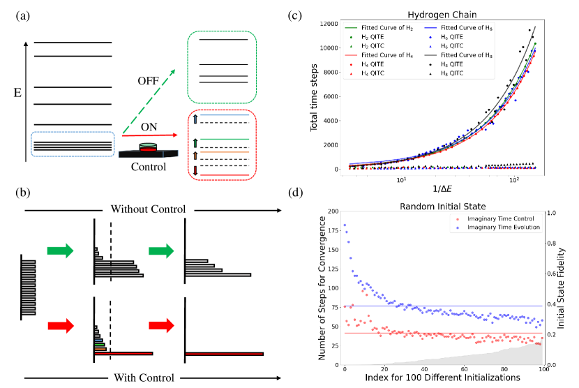
Figure 1: (a) A temporally modulated Hamiltonian to steer many-body quantum dynamics (b) The QITE gets slowed down significantly when the current state is the combination of many low-energy eigenstates. (c) The H-chain results for even Hydrogens that are scaled from $H_{2}$ to $H_{8}$. The dots of different colors indicate the total convergence steps of QITE and QITC in different systems, and lines of different colors indicate that the fitted curves of QITE satisfy $f(x)=ae^{x}+b$, where $x=log(1/\Delta E)$. On the other hand, the QITC results yielded $f(x)=ax+b$. (See the details in Supplementary Section B1) (d) The numerical results of 4 qubits $H_{2}$ molecule with bond length 0.74 and 100 random initial state, the x-axis is the case number we assign for randomly chosen initial points, the left y-axis is the number of convergence, and the right y-axis is the state fidelity between the initial state and ground state. The control Hamiltonian used here is single Pauli $Z$.

Quantum imaginary time control

A quantum system’s dynamical evolution under a time-dependent Hamiltonian in the imaginary-time domain is given by the modified time-dependent Schrodinger’s equation,

$$\frac{d\psi(\tau)}{d\tau}=-(H_{p}+\beta(\tau)H_{d}-E_{\tau})\psi(\tau),$$ (3)

where $\psi(\tau)$ is the system’s state vector, $H_{p}$ is the problem Hamiltonian, and $H_{d}$ is the control Hamiltonian coupled to a time-dependent control pulse $\beta(\tau)$. $E_{\tau}=\expectationvalue{(H_{p}+\beta(\tau)H_{d})}{\psi(\tau)}$ is the state’s expected energy, and it is introduced in Eq. 3 to ensure the time-evolved wave function will be properly normalized. According to the Lyapunov method and La Salle invariance principle [46], the state preparation problem can be re-formulated as an optimization problem in which the target state minimizes a Lyapunov function $V(\psi(\tau))$, which must satisfy the following conditions. Consider a system of differential equations $\dot{\psi}(\tau)=f(\psi(\tau))$ with a smooth $f$ and the state of the system satisfies the conservation of probability $||\psi(\tau)||=1,\forall\tau\geq 0$, which means that $\psi$ is on the unit sphere $\mathbf{S}=\{x\in\mathbf{C}^{n}:||x||=1\}$. Consider a smooth function $V(\psi)$ on the phase space $\Omega$, such that $V(\psi)\geq 0$ and $\frac{dV(\psi)}{d\tau}\leq 0$ for $\psi\in\Omega$. Let us define $\mathcal{M}$ to be the set of points $\psi\in\Omega$ such that $dV(\psi)/d\tau=0$, then every solution of the time-dependent Schrodinger’s equation converges to $\mathcal{M}$ as $t\rightarrow\infty$.

For the preparation of the ground state of a Hamiltonian, the Lyapunov function can be chosen as follows,

$$V(\psi(\tau))=\expectationvalue{P}{\psi(\tau)},$$ (4)

where $P=H_{p}-\tilde{E}$ with $\tilde{E}$ a constant shift of energy to ensure that $P$ is a semi-positive definite Hermitian operator[43]. The time derivative of the Lyapunov function in Eq.(4) reads,

$$\dot{V}(\psi) =2\sigma_{H_{p}}^{2}(\tau)-\beta(\tau)D(\tau),$$ (5)

where $\psi$ is an abbreviation for $\psi(\tau)$. The other variables are given by

$$\begin{array}[]{l}\sigma_{H_{p}}^{2}(\tau)\equiv\left\langle\psi\left|H_{p}\right|\psi\right\rangle^{2}-\left\langle\psi\left|H_{p}^{2}\right|\psi\right\rangle,\\ T(\tau)\equiv\left\langle\psi\left|\left\{H_{p},H_{d}\right\}\right|\psi\right\rangle-2\left\langle\psi\left|H_{p}\right|\psi\right\rangle\left\langle\psi\left|H_{d}\right|\psi\right\rangle,\end{array}$$ (6)

where $\{\cdot,\cdot\}$ is the anti-commutator. In this case, the Lyapunov-controlled quantum dynamics will be driven to the asymptotically stable points, which form the ground-state manifold, in $\mathcal{M}$. To make $\dot{V}(\psi)\leq 0$, it is sufficient to enforce $\beta(\tau)T(\tau)\geq 0$ as $\sigma_{H_{p}}^{2}(\tau)$ is less than or equal to zero. In summary, a successful imaginary-time control to prepare the ground state of a Hamiltonian is to design an appropriate $\beta(\tau)$ and suitable $H_{d}$ (see Supplementary Section A). For this work, we proposed some control strategies (see Method) that are inspired by the bang-bang and approximate bang-bang Lyapunov control that can provide rapid state transitions for quantum systems in the real-time domain[44].

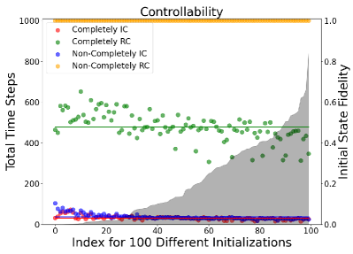
Figure 2: The numerical result of 2 qubits $H_{2}$ molecule (see Supplementary Section D), the x-axis is a serial number of initial states, the left y-axis is the convergent steps, the maximum number of steps is limited to 1000, and the right y-axis(corresponding to the grey area) is the initial and ground state overlap. The complete imaginary time control(Completely IC (red)), the non-completely imaginary time control(Non-Completely IC (blue)), and the complete real-time control(Completely RC (green)) could all converge in time. However, the non-completely real-time control(Non-Completely RC (yellow)) cannot converge in a limited time.

Comparison to imaginary time evolution

We find that QITE gets slowed down significantly when the current state is mainly a superposition of many densely spaced low-energy eigenstates Fig. 1(b). For the original $H_{p}$ the energy gap between the ground state and the first excited state remains fixed and limits the simulation efficiency. Consistent with the theoretical motivation stated before, we find that the QITC temporally modulates the entire spectrum of $H(\tau)$ during the evolution and finally returns back to the original spectrum of $H_{p}$. Those temporally enlarged energy gaps contribute to the acceleration of the simulation process, see Fig. 1(a)

In Fig. 1(c), we present the results of ground-state preparation, it shows that the QITC provides orders of magnitude speedup (suggesting exponential-like acceleration) in the rate of convergence with respect to the intra-molecular distance. Note that the $\Delta_{10}$ energy gap reduces when the intra-molecular distance grows. This observed scaling trend certainly benefits the simulation of large complex systems with small energy gaps. To ensure this observed significant speedup holds in a variety of chemical systems, we provide simulation results of four, eight, twelve, and sixteen-qubit Hydrogen chains, a twelve-qubit LiH, and HF in the following Section. In Fig. 1(d), we illustrate the enhanced convergence efficiency for the QITC with different initial states. These results also indicate that the convergence of the QITC does not sensitively depend on the initial states.

Comparison to the real-time control for the ground-state preparation

An essential question for a driven state preparation concerns the controllability for the given control Hamiltonians $\{H_{d}^{0},H_{d}^{1},...\}$, i.e. whether the quantum system can be driven to the ground state of $H_{p}$ from any given initial state when it is subjected to evolve under the time-dependent Hamiltonian $H(\tau)=H_{p}+\beta(\tau)H_{d}$ in our context, where $H_{d}=\sum_{i}\beta^{i}(\tau)H_{d}^{i}$. Without loss of generality, we write $\beta(\tau)H_{d}$ as opposed to the more general form $\sum_{i}\beta^{i}(\tau)H_{d}^{i}$ throughout this work. This simple question for real-time control turns out to be rather difficult to answer for a large quantum system. A common technique involves analysis of the structure and rank of corresponding Lie groups and algebra for the propagators[40, 41, 45]. It is computationally demanding to determine the controllability of a particular setup, and it is unlikely that a random selection of control Hamiltonians can guarantee complete controllability. The challenge to select an appropriate set of control Hamiltonians (with respect to a given initial state) poses a severe challenge to derive a practical real-time control strategy to prepare a target ground state.

The same question regarding controllability admits a much clearer answer in the imaginary-time domain. As long as the imaginary-time-evolved state $\psi(\tau)$ and the ground state have a non-zero overlap, the system can always converge to the ground state in a sufficiently long evolution time. Hence, a more crucial question is whether a set of control Hamiltonians along with the corresponding control strategy $\beta(\tau)$ (i.e. to ensure $\dot{V}(\psi)\leq 0$) can substantially accelerate the driving from a given initial state to the ground state of $H_{p}$. As discussed next, the imaginary-time Lyapunov control can indeed work with a broader range of control Hamiltonians for accelerating the ground-state preparations.

We further illustrate the differences between real-time and imaginary-time Lyapunov control with a numerical example involving $H_{2}$ molecule in Fig. 2. We randomly choose 100 initial states and examine how long the real-time and imaginary-time evolutions converge to the ground state under control Hamiltonians with various degrees of controllability. When the control Hamiltonian satisfies the strongly complete controllability[42], we expect that the driven dynamics converge to the ground state without difficulty. While this expectation holds in the numerical experiments, we find the imaginary-time evolution converges much faster (with roughly one-tenth of the time steps for the real-time evolution on average). We expect this performance gap to be further enlarged with the system size. For control Hamiltonians with incomplete controllability, the imaginary-time control can still lead to satisfactory convergence in a small number of time steps. In contrast, the real-time simulation under the same control Hamiltonians cannot converge for all 100 initial states in the pre-defined maximum number of steps allowed.

Comparing QITC and VQE in Noisy Environment

To make the method accessible in the noisy intermediate-scale quantum era, we further propose a variational form of the algorithm that could work with shallow quantum circuits.

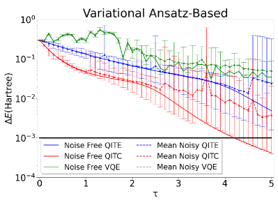
Figure 3: The numerical results of 4-qubit Hydrogen molecule (see Supplementary Section D) with a bond length of 0.74$\r{A}$. The x-axis is imaginary time with a single time-step $\Delta\tau=0.1$ and the total time step is 50. The y-axis is the energy difference from ground-state energy. The solid line is the result of the numerical noise-free model (the black line is chemical accuracy). The numerical noisy model is simulated by adding the single qubit depolarization error channels with parameter $\lambda=10^{-4}$ and the CNOT depolarization error channels with parameter $\lambda=10^{-5}$ (We use TensorCircuit[51] to effectively get this result.). The dashed line is the mean value of 50 noisy results, and the error bar is bounded by the worst and best simulation results. The control strategy used in this simulation is approximately bang-bang control with $S=0.3$ and $\gamma=5$.

In this section, we compare the simulation ability of VQE, variational imaginary time evolution, and variational imaginary time control. In Fig. 3, we compare the results among the VQE, the variational ansatz-based QITE, and the variational ansatz-based QITC for the ground-state preparation of a 4-qubit $H_{2}$ system under both noise-free and noisy situations. We adopt the fully connected ansatz with high expressibility[25] initialized by the same random initial parameters for all the methods. The results show that the QITC converges faster than the QITE and the VQE for both the noisy and noise-free models. The control Hamiltonian we using here is the single Z and double Z selected from the hydrogen Hamiltonian $H_{p}$.

Model	$(1\times 1)$	$(2\times 2)$	$(3\times 3)$	$(2\times 2)_{D}$
h/J	0.1/0.09	0.1/0.09	0.1/0.09	0.2/0.1
QITE total time step	366	764	5963	28934
QITC total time step	130	253	1137	182
Difference	236	511	4826	28752
Ratio	2.82	3.02	5.24	158.98
Control	ZIIZ	ZIIZ	ZIIZ	ZIIZ
Hamiltonian ($H_{d}$)		ZIZ	ZZZ	ZZZ
Number of $H_{d}$	4	18	32	18

Table 1: The result of 2D Heisenberg model. The $(2\times 2)_{D}$ is the ’difficult’ regime in the space of Hamiltonian parameters case where QITE required a great number of steps to converge. All the control Hamiltonians are in the structure of simple Pauli $Z$ with the cyclic structure mentioned above and we only write down the non-trivial part of Pauli in the table. For example, the ZIZ in the 2×2 model is the abbreviation of ZIZIIIIII. The number of control steps for all cases is 100 steps.

Examples Beyond H Chains

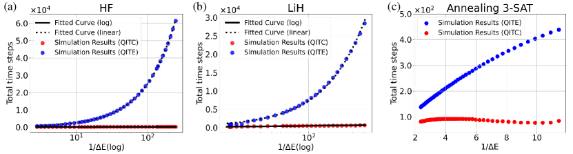
Figure 4: (a)The numerical result of 12 qubits HF molecule (see Supplementary Section D) with bond length from 1.00 to 2.36 ${\AA}$ and the same initial state with equal superposition of all the basis states, the QITE is the result of imaginary time evolution. The QITC is the result of the imaginary time control, the x-axis refers to the log of one over the energy gap between the ground state and the first excited state, and the y-axis is the total time step. QITE fitted curve f(x)=248.67 exp(x) + 126.12 and QITC fitted curve f(x)=12.80 x+ 110.09, where $x=log(1/\Delta E)$. (b) The result of LiH problem. The x-axis is log of one over energy gap between the ground state and the first excited state. The y-axis is the total time steps of the ITE and ITC. QITE fitted function f(x)=71.60 exp(x) + 154.96 and QITC fitted curve f(x)=125.31 x – 108.81, where $x=log(1/\Delta E)$. (c)The result of 3-SAT quantum annealing problem. The x-axis is the one over the energy gap between the ground state and the first excited state. The y-axis is the converge steps difference between the ITE and ITC.

First, we simulate two diatomic molecules HF and LiH to test the speedup from the control in molecule systems. In Fig. 4 (a-b), we show that both the HF and LiH using the same control Hamiltonian used in the H-chain system can obtain exponential-like speedup. Second, we consider a spin model constructed from the annealing solving of an 11-qubit 3-SAT problem during the linear schedule, see $H(s)$ defined in Supplementary Section B3. We then implement and compare the simulations of the ITC and the ITE in order to prepare the ground states for a series of $H(s)$ chosen along the adiabatic path. According to the simulation result in Fig. 4 (c), we numerically verify the speed-up of the ITC as the instantaneous energy gap $\Delta E(s)$ shrinks. Third, we demonstrate the 2D Heisenberg model (see Hamiltonian details in the Method Section) with different system sizes using control Hamiltonian constructed only by Pauli $Z$ up to cube order. As we can see from the results in Table 1, Lypapunov control provides obvious speed-up while the system size scales up. The $(2\times 2)_{D}$ case also indicates the existence of great speed-up using simple control Hamiltonian Pauli $Z$.

Finally, we simulate a 4-qubit variational-ansatz based imaginary time evolution of the spin glass model (see Hamiltonian details in the Method Section) in Fig. 5 with random variables $J_{ij}=(0.049,0.215,0.103,0.045,-0.076,0.146)$, the energy difference between the ground state and first excited state $\Delta_{10}$, in this case, is 0.22 which is not small compared to the result of our molecule models. Although the QITE can work fine with such $\Delta_{10}$, it is still difficult to find a good initial state for a complex system like this SK model. To prepare a better initial state, we use VQE with COBYLA optimizer and variational QITC with commute basis $H_{d}=\{XXXX,YYYY,ZZZZ\}$ at the first ten steps respectively. After the initial state preparation, we use variational imaginary time evolution to evolve to the ground state given these two initial states. It can be seen that compared with the VQE initial state, the control initial state can achieve higher accuracy under the same number of convergence steps. The details and more discussion of the models are presented in Supplementary Section B.

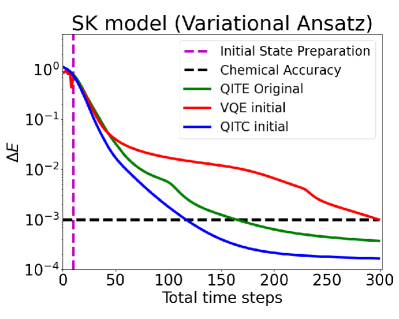
Figure 5: The result of 4 qubits SK model. The x-axis is the number of time steps and the y-axis is the energy difference from the ground state. The control initial can achieve chemical accuracy around three times faster than the VQE initial with a smoother convergence path.

Resource Consumption for scaling H-chain system

So far, we have only discussed the conceptual advantage of our method (i.e. faster convergence towards the ground state). As we propose this method in the context of digital quantum simulation on a quantum computer, we further analyze how our method helps to reduce the consumption of quantum resources. Here we present the number of measurements for $H_{2},H_{4},H_{6}$ and $H_{8}$ (i.e. 4, 8, 12, and 16 qubits)). In Fig. 6, we summarize this reduction in the number of measurements with different choices of $H_{d}$(see Supplementary Section B for details): The Full $H_{d}$ with the same $1/\Delta E$(blue bar), the Half $H_{d}$ with same $1/\Delta E$(orange bar), the Full $H_{d}$ with the same bond length(green bar) and the Half $H_{d}$ with the same bond length(red bar). The result shows that all of them give some polynomial reductions in the number of measurements, compared to the standard variational ansatz-based imaginary time evolution. This is because the extra measurement numbers from ${H_{d},H_{p}}$ are relatively small in comparison to the variational ansatz update measurements, which scales as $N_{p}N_{\theta}$, where $N_{p}$ is the number of Pauli terms of $H_{p}$ and $N_{\theta}$ is the number of the parameter in the ansatz circuit (we used k-UpCCGSD from PennyLane for the reference). In Table 2 we show the $N_{p}$, $N_{\theta}$, and extra measurements for different $H_{d}$. Thus, according to Fig. 6, for the molecules tested in this study, we find the measurement resource reduction increases polynomially with the system size.

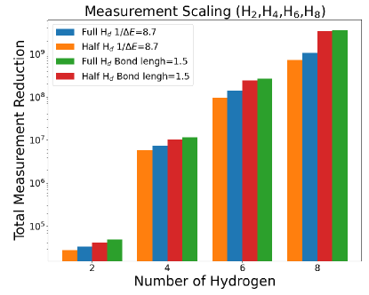
Figure 6: Total measurement difference results. The results are the estimation of the difference in total measurements for imaginary time evolution and imaginary time control convergence, the calculation details are listed in Table 2. The x-axis is the number of H in the system and the y-axis is the log plot of the measurement reduction. The Full $H_{d}$ and Half $H_{d}$ are listed in Supplementary Section B.

	$N_{p}$	$N_{\theta}$ k-UpCCGSD	$N_{p}N_{\theta}$	Full Hd		Half Hd		Same Bond Length
				$\{H_{d},H_{p}\}$	$\Delta Step$	$\{H_{d},H_{p}\}$	$\Delta Step$	$\Delta Step_{f}$	$\Delta Step_{h}$
$H_{2}$	15	6 (k=1)	90	5	381	5	327	554	473
$H_{4}$	185	72 (k=2)	13320	1006	555	577	449	872	771
$H_{6}$	919	270 (k=3)	248130	16627	572	8804	399	1098	991
$H_{8}$	2913	672 (k=4)	1957536	112396	544	57966	377	1804	1712

Table 2: Summary of Measurement Test, where $N_{p}$ is the number of Pauli terms of problem Hamiltonian $H_{p}$ (here we use Jordan-Wigner transformation), $N_{\theta}$ is the number of parameters in the ansatz circuit (here we use k-UpCCGSD) and $N_{p}N_{\theta}$ is the number of measurement to update the variational-ansatz based imaginary time evolution. $\{H_{p},H_{d}\}$ is the extra measurement for update control Hamiltonian coefficient $\beta(\tau)$ and $\Delta Step$ are the total time step difference between imaginary time evolution and imaginary time control. The $\Delta Step_{f}$ and $\Delta Step_{h}$ are the total time step difference using Full $H_{d}$ control and Half $H_{d}$ control for same bond length case.

Discussion

In summary, we propose to utilize the imaginary-time Lyapunov control to prepare ground states and explain the advantages of QITC. First, imaginary time control can speed up imaginary time evolution with the proper design of control Hamiltonian and control function $\beta(\tau)$. Through numerical experiments on a broad spectrum of realistic models, we show that compared to standard imaginary-time evolution, imaginary-time control provides substantial speed-up for all systems. And for the selected small-gap systems invested in this work, an exponential-like speedup is observed. Secondly, compared to real-time control, imaginary-time control admits more relaxed conditions for controllability (when the target is the ground state) and a broader range of control Hamiltonians to facilitate the desired state transitions in a finite time. Thirdly, to make the present method accessible in the NISQ era, we propose a variational simulation of the QITC with an ansatz circuit. Finally, we show various examples to strengthen the speedup from QITC. We also show that when the control Hamiltonian is chosen appropriately, it does not incur many additional measurement costs and exhibits higher robustness against noises. These merits make the present approach a natural replacement for the variational ground-state preparation. For future work, we aim to study imaginary time control for other challenging state preparation tasks, such as excited states simulation and Gibbs state preparation, etc.

Methods

In this section, we present the details of the variational algorithm for QITE simulations, studied spin-model Hamiltonian, and the imaginary time control strategies.

Variational algorithm for QITE simulations

To utilize the proposed imaginary-time control to prepare a ground state on a near-term quantum device, we rely on the time-dependent variational principle to approximate the evolution of the QITC as sequential updates of parameters for an ansatz circuit, as first proposed by McArdle et al.,[16] for the QITE. The modified algorithm proceeds as follows. Given a time-dependent Hamiltonian $H(\tau)=H_{p}+\beta(\tau)H_{d}$, we would invoke the the McLachlan’s variational principle[48, 49],

$$\delta||(\partial/\partial\tau+H(\tau)-E_{\tau})\ket{\psi(\tau)}||=0,$$ (7)

which conducting the dynamic evolution $\partial\left|\psi(\tau)\right>/\partial\tau=-\left[H(\tau)-E_{\tau}\right]\left|\psi(\tau)\right>$ by deducing the incremental update (corresponding to one time step $\delta\tau$) of the parameters $\theta$ for an ansatz circuit. Following Ref. [16], we need to solve the following equations,

$$\sum_{j}A_{ij}\dot{\theta_{j}}=C_{i},\forall i$$ (8)

where,

$$\begin{array}[]{c}A_{ij}=\real\left(\frac{\partial\langle\phi(\tau)|}{\partial\theta_{i}}\frac{\partial|\phi(\tau)\rangle}{\partial\theta_{j}}\right)\\ C_{i}=\real\left(-\sum_{\alpha}\lambda_{\alpha}\frac{\partial\langle\phi(\tau)|}{\partial\theta_{i}}h_{\alpha}|\phi(\tau)\rangle\right.\end{array}$$ (9)

and $h_{\alpha}$ and $\lambda_{\alpha}$ are the Pauli terms and coefficients of the Hamiltonian $H=H_{p}+\beta(\tau)H_{d}=\sum_{\alpha}\lambda_{\alpha}(\tau)h_{\alpha}$. With the new ansatz state, we can then evaluate the Lyapunov function and assign values to the pulse $\beta(\tau)$ via a pre-determined control rule to keep $\dot{V}(\psi)<0$. The procedure of alternating updates of $\theta$ and $\beta$ is then repeated until a fixed point is reached.

Hamiltonian details for the spin models

The 2D Heisenberg models are constructed with non-periodic boundary conditions, whose Hamiltonian can be written as

$$H_{p}=h_{i}\sum_{i}Z^{i}+J_{ij}\sum_{edge}X^{i}X^{j}+Y^{i}Y^{j}+Z^{i}Z^{j}.$$

The model information in the table presents edge $\times$ edge, for example, $2\times 2$ means $3\times 3$ lattice. The Hamiltonian of Sherrington–Kirkpatrick model we use can be written as

$$H_{p}=\sum_{i<j}J_{ij}(X^{i}X^{j}+Y^{i}Y^{j}+Z^{i}Z^{j})$$

, with random generate variables $J_{ij}\in(-0.5,0.5)$ and using $\ket{++\dots+}$ as the initial state.

The imaginary time Control Strategy

In this section, we will discuss the approximate bang-bang control and bang-bang control laws we use to design the $\beta(\tau)$ for imaginary time control and the inverse control strategy we used to accelerate our molecule system ground state convergence. To appreciate our approach, we first review some typical real-time control strategies designed to guarantee $\dot{V}\leq 0$. Following a standard convention [44], we refer to the following choice as the standard Lyapunov control,

$$\beta_{k}(t)=-K_{k}T_{k}(t),$$

where $\beta_{k}(t)$ is an external real-valued control field, $K>0$ is the control gain used to adjust the amplitude of the control field, and $T_{k}(t)\equiv(\expectationvalue{i[H_{d},H_{p}]}{\psi}$ for the real-time control. Another commonly used strategy is the bang-bang Lyapunov control,

$$\beta_{k}(t)=\left\{\begin{array}[]{rcl}-S,&&(T_{k}>0)\\ S,&&(T_{k}<0)\quad k=1,...,m,\\ 0,&&(T_{k}=0)\end{array}\right.$$

where $S>0$ is the maximum strength of the control field. In order to achieve a good trade-off between convergence and the rapidity of control, Kuang et al.[44] propose an approximate bang-bang control as follows,

$$\beta_{k}(t)=\frac{2S}{1+e^{-\gamma T_{k}}}-S.$$

where $\gamma>0$ is a parameter used to adjust the hardness of the control strategy. For the imaginary time control strategy, let us generalize the standard Lyapunov control such that it could work with the imaginary-time evolution. We redefine $T_{k}\equiv 2\expectationvalue{H_{p}}{\psi}\expectationvalue{H_{d}}{\psi}-\expectationvalue{\{H_{p},H_{d}\}}{\psi}$ in this case. The $H_{d}$ related terms in $T_{k}(\tau)$ may entail lots of extra measurements if they cannot be obtained by measuring the Pauli terms appearing in $\expectationvalue{H_{p}}{\psi}$. To reduce the measurement cost and still maintain a powerful $H_{d}$ to provide an enhanced convergence, we propose the following strategy. We first decide if the state in the quantum circuit has high overlap with any eigenstate of $H_{p}$ or $H_{d}$ by checking the value of $T_{k}$, if $T_{k}<L$ then we do not apply any control pulses, otherwise we use a similar control strategy for the real-time case introduced above.

$$\beta_{k}(\tau)=\left\{\begin{array}[]{rcl}&\frac{2S}{1+e^{-\gamma T_{k}}}-S,&(T_{k}\geq L)\\ &0,&else\end{array}\right.$$

where L is some pre-defined threshold value. If the state is close to an eigenstate (i.e. $T_{k}(\tau)<L$), we should turn off the control field and let the system evolves under $H_{p}$ in the imaginary-time domain. This truncation can greatly reduce the measurement costs (for the implementation of the corresponding variational algorithm) in the region where the state will linearly converge to the eigenstate. Finally, we test how the truncation (i.e. setting $\beta_{k}(\tau)=0$ when $T_{k}(\tau)<L$) will affect the precision of the converged results given by truncating the control pulse, and we also test the control with different phases in Supplementary Section C.

Author contributions statement

Y.C. designed and implemented the quantum algorithms. All authors contributed to interpreting data and engaged in useful scientific discussions. All authors reviewed the manuscript.

Additional information

To include, in this order: Accession codes (where applicable); Competing interests (mandatoery statement).

The corresponding author is responsible for submitting a competing interests statement on behalf of all authors of the paper. This statement must be included in the submitted article file.

References

- [1] Monz, T.et al. "Realization of a scalable Shor algorithm." Science 351.6277, 1068-1070(2016).
- [2] Schaden, M. "Quantum finance." Physica A: Statistical Mechanics and Its Applications 316.1-4, 511-538(2002).
- [3] Biamonte, J.et al. "Quantum machine learning." Nature 549.7671, 195-202(2017).
- [4] McArdle, S.et al. "Quantum computational chemistry." Reviews of Modern Physics 92.1, 015003(2020).
- [5] Bauer, B.et al. "Quantum algorithms for quantum chemistry and quantum materials science." Chemical Reviews 120.22, 12685-12717(2020).
- [6] Peruzzo, A.et al. "A variational eigenvalue solver on a photonic quantum processor." Nature communications 5.1, 1-7(2014).
- [7] Grimsley, H.et al. "An adaptive variational algorithm for exact molecular simulations on a quantum computer." Nature communications 10.1, 1-9(2019).
- [8] Higgott, O., Wang, D. & Brierley, S. "Variational quantum computation of excited states." Quantum 3, 156(2019).
- [9] Cerezo, M.et al. "Variational quantum algorithms." Nature Reviews Physics, 1-20(2021).
- [10] Kitaev, A. "Quantum measurements and the Abelian stabilizer problem." Preprint at http://arXiv.org/quant-ph/9511026 (1995).
- [11] Dobšíček, M.et al. "Arbitrary accuracy iterative quantum phase estimation algorithm using a single ancillary qubit: A two-qubit benchmark." Physical Review A 76.3, 030306(2007).
- [12] Wiebe, N, & Granade, C. "Efficient Bayesian phase estimation." Physical review letters 117.1, 010503(2016).
- [13] O’Brien, T.E., Brian, T., and Barbara M. T. "Quantum phase estimation of multiple eigenvalues for small-scale (noisy) experiments." New Journal of Physics 21.2, 023022 (2019).
- [14] Gomes, N.et al. "Efficient step-merged quantum imaginary time evolution algorithm for quantum chemistry." Journal of Chemical Theory and Computation 16.10, 6256-6266(2020).
- [15] Motta, M.et al. "Determining eigenstates and thermal states on a quantum computer using quantum imaginary time evolution." Nature Physics 16.2, 205-210(2020).
- [16] McArdle, S.et al. "Variational ansatz-based quantum simulation of imaginary time evolution." npj Quantum Information 5.1, 1-6(2019).
- [17] Yuan, X.et al. "Theory of variational quantum simulation." Quantum 3, 191(2019).
- [18] Beach, M.J.S, et al. "Making trotters sprint: A variational imaginary time ansatz for quantum many-body systems." Physical Review B 100.9, 094434(2019).
- [19] Seki, K. & Yunoki, S. "Quantum power method by a superposition of time-evolved states." PRX Quantum 2.1 (2021): 010333.
- [20] Kyriienko, O. "Quantum inverse iteration algorithm for programmable quantum simulators." npj Quantum Information 6.1, 1-8(2020).
- [21] Childs, A.M.et al. "Theory of trotter error with commutator scaling." Physical Review X 11.1, 011020(2021).
- [22] Grimsley, H.R. et al. "Is the trotterized uccsd ansatz chemically well-defined?." Journal of chemical theory and computation 16.1, 1-6(2019).
- [23] Lee, J.et al. "Generalized unitary coupled cluster wave functions for quantum computation." Journal of chemical theory and computation 15.1, 311-324(2018).
- [24] Kandala, A. et al. "Hardware-efficient variational quantum eigensolver for small molecules and quantum magnets." Nature 549.7671, 242-246(2017).
- [25] Sim, S., Peter, D.J.& Aspuru-Guzik, A. "Expressibility and entangling capability of parameterized quantum circuits for hybrid quantum-classical algorithms." Advanced Quantum Technologies 2.12, 1900070(2019).
- [26] McClean, J.R.et al. "Barren plateaus in quantum neural network training landscapes." Nature communications 9.1, 1-6(2018).
- [27] Grant, E.et al. "An initialization strategy for addressing barren plateaus in parametrized quantum circuits." Quantum 3, 214(2019).
- [28] Cerezo, M. et al. "Cost function dependent barren plateaus in shallow parametrized quantum circuits." Nature communications 12.1, 1-12(2021).
- [29] Wang, S.et al. "Noise-induced barren plateaus in variational quantum algorithms." Nature communications 12.1, 1-11(2021).
- [30] Holmes, Z.et al. "Barren plateaus preclude learning scramblers." Physical Review Letters 126.19, 190501(2021).
- [31] Kuang, S. & Shuang C. "Lyapunov control methods of closed quantum systems." Automatica 44.1, 98-108(2008).
- [32] Wang, X. & Sophie G.S. "Analysis of Lyapunov method for control of quantum states." IEEE Transactions on Automatic Control 55.10, 2259-2270(2010).
- [33] Dong, D. & Petersen, I.R. "Quantum control theory and applications: a survey." IET Control Theory & Applications 4.12, 2651-2671(2010).
- [34] Cong, S & Fangfang M. "A survey of quantum Lyapunov control methods." The Scientific World Journal 2013 (2013).
- [35] Magann, A.B.et al. "Feedback-based quantum optimization." Preprint at https://arxiv.org/abs/2103.08619(2021).
- [36] Magann, A.B.et al. "Digital quantum simulation of molecular dynamics and control." Physical Review Research 3.2, 023165(2021).
- [37] Ramakrishna, V.et al. "Controllability of molecular systems." Physical Review A 51.2, 960(1995).
- [38] Chen, Y.et al. "Optimizing quantum annealing schedules: From Monte Carlo tree search to quantumzero." Preprint at https://arxiv.org/abs/2004.02836(2020).
- [39] Ran, D. et al. "Speeding up adiabatic passage by adding Lyapunov control." Physical Review A 96.3, 033803(2017).
- [40] Schirmer, S.G., Fu, H. & Solomon,A.I. "Complete controllability of quantum systems." Physical Review A 63.6, 063410(2001).
- [41] Albertini, F. & D’Alessandro, D."Notions of controllability for bilinear multilevel quantum systems." IEEE Transactions on Automatic Control 48.8, 1399-1403(2003).
- [42] Zhang, C., Dong, D.& Chen, Z. "Control of non-controllable quantum systems: a quantum control algorithm based on Grover iteration." Journal of Optics B: Quantum and Semiclassical Optics 7.10, S313(2005).
- [43] Grivopoulos, S., & Bamieh, B. (2003, December). Lyapunov-based control of quantum systems. In 42nd IEEE International Conference on Decision and Control (IEEE Cat. No. 03CH37475) (Vol. 1, pp. 434-438). IEEE.
- [44] Kuang, S., Dong, D., & Petersen, I. R. (2014, November). Approximate bang-bang Lyapunov control for closed quantum systems. In 2014 4th Australian Control Conference (AUCC) (pp. 124-129). IEEE(2014).
- [45] Huang, G.M., Tarn, T. & Clark, J. "On the controllability of quantum-mechanical systems." Journal of Mathematical Physics 24.11, 2608-2618(1983).
- [46] D’Alessandro, D. Introduction to quantum control and dynamics. Chapman and hall/CRC (2021).
- [47] Schuld, M.et al. "Evaluating analytic gradients on quantum hardware." Physical Review A 99.3, 032331(2019).
- [48] McLachlan, A.D. "A variational solution of the time-dependent Schrodinger equation." Molecular Physics 8.1, 39-44(1964).
- [49] Broeckhove, J.et al. "On the equivalence of time-dependent variational principles." Chemical physics letters 149.5-6, 547-550(1988).
- [50] del Campo, A, Rams, M. & Zurek, W. "Assisted finite-rate adiabatic passage across a quantum critical point: exact solution for the quantum Ising model." Physical review letters 109.11 (2012): 115703.
- [51] Zhang, S.et al. "TensorCircuit: a Quantum Software Framework for the NISQ Era." Preprint at https://arxiv.org/abs/2205.10091(2022).
Acknowledgements
AH gratefully acknowledges the sponsorship from the City University of Hong Kong (Project No. 7005615); and the Hong Kong Institute for Advanced Study, City University of Hong Kong (Project No. 9360157). The work described in this paper was substantially supported by a grant from the Research Grants Council of the Hong Kong Special Administrative Region, China (Project No. CityU 11200120).