2+1 flavor fine lattice simulation at finite temperature with domain-wall fermions

Abstract

Simulations for the thermodynamics of the 2+1 flavor QCD are performed employing chiral fermions. The use of Möbius domain-wall fermions with stout-link smearing is more effective on the finer lattices where all the relevant chiral symmetries are realized more accurately. We report on the initial simulations near the (pseudo) critical point using the line of constant physics with an average $ud$ quark mass slightly heavier than physical at $a\lesssim 0.1$ fm.

YITP-21-151

1 Introduction

Nature of the phase transition of $2+1$-flavor QCD is a prime interest as it provides a good approximation of what happens in the real world when the temperature gets high enough to liberate the quark degree of freedom. Especially the “physical point” simulations, where the degenerate $ud$ quark mass is set as their average physical value and strange quark mass is tuned to physical, are useful and have direct relevance for the understanding of the history of the universe and physics in the heavy ion/high energy experiments. These days there have emerged much interests in investigating, not only the physical point, but also extended region like fictitious $ud$ chiral limit. More in general, the phase structure of the Columbia plot is getting match attention [1, 2, 3].

Here we report on the newly started project aiming to study the thermodynamics near the physical point in the Columbia plot using a chiral fermion formulation. There was a study by HotQCD collaboration using domain-wall fermions at a course lattice (with the temporal extent $N_{t}=8$) [4]. In the studies by JLQCD for $2$-flavor ($N_{f}=2$) QCD [5, 6, 7] it is shown that the fine lattice simulations are indispensable to maintain the underlining symmetries $SU(2)$ and $U(1)$ chiral, especially to study the fate of $U(1)_{A}$. To understand the phase structure near the $ud$ chiral limit it would be important have good control of these symmetries as the fate of the symmetries could change the order of the transition [8]. This made us plan the $N_{f}=2+1$ flavor simulations using the same setup as $N_{f}=2$, which uses Möbius domain-wall fermions [9] (scale-factor-2 Shamir-type fermions) with the stout-link smearing in the Wilson kernel. Some $N_{f}=2+1$ studies have already been done following the same strategy as $N_{f}=2$ where the gauge coupling is fixed and the “ud” mass is changed. The preliminary results have been reported in this conference [10]. Yet another project using the same action, but with a line of constant physics to change only the temperature, has been started.

In this report, our main focus is to discuss how we obtain and use the line of constant physics of the action we use for the $N_{f}=2+1$ QCD. In these studies we fix the domain-wall fermion parameters: the domain-wall height as $M_{5}=1$ as usual in JLQCD and the 5th dimension size as $L_{s}=12$. After discussing these setup, some early and preliminary results are shown.

2 Scale setting and line of constant physics

We would like to express the lattice spacing and physical strange quark mass point as functions of the gauge coupling $\beta$: $a(\beta)$ and $m_{s}(\beta)$, where the latter is the strange quark mass in the lattice action. The ratio of strange and average $ud$ quark mass is known and we can obtain the lattice $m_{ud}(\beta)$ using the ratio.

2.1 Lattice spacing

We restrict the lattice spacing to be used in this finite temperature study not to be far away from the region used in the zero temperature JLQCD studies. These include the coarsest lattices generated only for an unpublished pilot study $a\simeq 0.095$ fm, as well as finer lattices: $a\simeq 0.08$, $0.055$, $0.044$ fm. These lattice spacings are determined using $t_{0}$. In this way we can avoid performing expensive extra zero temperature simulations as much as possible. The left panel of Fig. 1 shows the results of the lattice spacing.

Figure 1: Lattice spacing as a function of $\beta$ (left) and lattice spacing divided by two-loop scaling as a function of an effective lattice spacing squared (right).

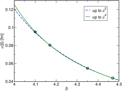
There is a method often used to parameterize the lattice spacing as a function of the gauge coupling using two-loop beta function with correction terms proposed by Edwards et al [11],

$$a=c_{0}f(g^{2})(1+c_{2}\hat{a}(g)^{2}+c_{4}\hat{a}(g)^{4}).$$ (1)

where

$$\hat{a}(g) \equiv \frac{f(g^{2})}{f(g_{0}^{2})},$$ (2)

$$f(g^{2}) \equiv (b_{0}g^{2})^{-b_{1}/2b_{0}^{2}}\exp\left(-\frac{1}{2b_{0}g^{2}}\right),$$ (3)

$$b_{0} = \frac{1}{(4\pi)^{2}}\left(11-\frac{2}{3}N_{f}\right),\;\;\;b_{1}=\frac{1}{(4\pi)^{4}}\left(102-\frac{38N_{f}}{3}\right),$$ (4)

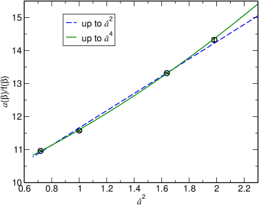
$g^{2}=6/\beta$, $N_{f}=3$, $c_{0}$, $c_{2}$ and $c_{4}$ are free parameters of the fit. We set the reference gauge coupling $g_{0}$ from the $\beta$ value of the second finest lattice $g_{0}^{2}=6/4.35$. $f(g^{2})$ expresses the scaling from the two-loop beta function, which is scheme independent. Beyond two loop, scheme dependence appears and is not convenient for this purpose. The $c_{2}$ and $c_{4}$ terms are meant to absorb the lattice discretization error. But, in practice they are also playing the role of absorbing the remnant RG scaling beyond two loop, which can be seen in the right panel of Fig. 1, where $a/f(g^{2})$ is plotted as a function of $\hat{a}^{2}$. The variation from 11 to 14 is too large to be regarded as a discretization error for domain-wall fermions at $a<0.1$ fm. Apart from the role of each terms one wants to check the effectiveness of the formula by looking at this figure. If the linearity is good one does not have to include $\hat{a}^{4}$ term in Eq. 1 to parameterize the lattice spacing. While it turns out that the linearity is marginally good, the fit (shown as dashed line) results in large $\chi^{2}/dof=6.6$. Therefore, we shall adopt the parameterization using up to $\hat{a}^{4}$ (shown as solid line) which gives $\chi^{2}/dof=1.6$. Resulting $a(\beta)$ parameterizations have been shown in Fig. 1.

The simulation range for our coarser lattice include $\beta=4.0$ as the lower edge. The $a(\beta)$ there is an extrapolation and has up to a few percent systematic uncertainty, estimated through an experiment of omitting the coarsest data to check how the two fits work at the coarsest data point.

2.2 Quark mass

The values of strange and average up, down quark masses are known to a good precision. To obtain the line of constant physics given the parameterization of the lattice spacing $a(\beta)$ in the previous subsection, we use the strange quark mass input using the relation,

$$m_{q}^{R}=Z_{m}m_{q}^{latt}\cdot a^{-1}(\beta),$$ (5)

where $m_{q}^{R}$ is the dimension-full renormalized quark mass of flavor $q$. We shall use $\overline{\mbox{MS}}$ scheme at the renormalization scale $\mu=2$ GeV for the renormalization constant $Z_{m}$. Once a parameterization of the quark mass renormalization factor $Z_{m}(\beta)$ is obtained, $m_{q}^{latt}(\beta)$ (multiplicatively renormalizable mass in lattice units) may be computed. This is a method alternative to the commonly-used hadron-mass input.

We shall use the following numbers for the quark masses for the $N_{f}=2+1$ physical point:

$$m_{s}^{R} = 92\;\mbox{MeV}$$ (6)

$$m_{s}^{R}/m_{ud}^{R} = 27.4,$$ (7)

based on the FLAG2019 averages [12]: $m_{s}^{R}=92.0(1.1)$ and $m_{s}^{R}/m_{ud}^{R}=27.42(12)$.

To determine the bare quark mass $m_{q}$ in the domain-wall fermion action, the residual mass $m_{res}$ due to a finite 5th dimension needs to be subtracted,

$$m_{q}^{latt}=m_{q}+m_{res}.$$ (8)

For $\beta\geq 4.17$ the residual mass is $m_{res}\lesssim 1$ MeV, which is about the same size of the error in $m_{s}^{R}$. Therefore we can safely neglect the effect of $m_{res}$ for the strange quark mass there. The physical $ud$ quark mass is larger than the residual mass, $m_{ud}^{R}>m_{res}$. However, the size is comparable as we will see below.

We use $Z_{m}$ obtained for the three finer lattice spacings [13] and parameterize that as a smooth function of $\beta$. Fig. 2 shows the measured $Z_{m}$ and its parameterization $Z_{m}(\beta)$ using a method described below.

Figure 2: Renormalization factor plotted as a function of $\beta$ at $2$ GeV (black) and that run to $\mu=a^{-1}$ using $\overline{\mbox{MS}}$ NNNLO running. Interpolation for the red squares is done through the fit with second-order polynomial in $g^{2}\propto\beta^{-1}$. Then it is run again to $\mu=2$ GeV using the $a(\beta)$ parameterization with $O(\hat{a}^{4})$.

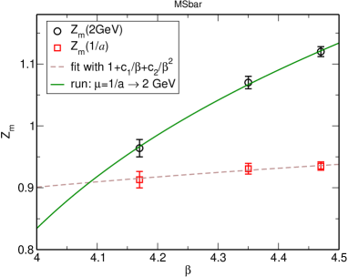
Let us first determine $Z_{m}$ at the scale $\mu=a^{-1}$ run from $\mu=2$ GeV, expecting the large log effect ($\log(a\mu)$) is removed. The RG running is performed using NNNLO [14] in $\overline{\mbox{MS}}$ scheme. Resulting $Z_{m}(a^{-1})$, which are shown as red squares, have less $\beta$ dependence. This $Z_{m}(a^{-1})$ may well be expressed in a polynomial of $g^{2}$ with $Z_{m}(a^{-1})\to 1$ in the continuum limit

$$Z_{m}(a^{-1})=1+\hat{c}_{1}g^{2}+\hat{c}_{2}g^{4}+\cdots.$$ (9)

Therefore we adopt a fit which is an expansion in $\beta^{-1}$,

$$Z_{m}(a^{-1})=1+c_{1}\beta^{-1}+c_{2}\beta^{-2}.$$ (10)

The fit result is shown as a brown dashed line. From this result one can obtain $Z_{m}(2\ \mbox{GeV})$ at arbitrary $\beta$ values by applying the NNNLO running, which are shown as a green solid line obtained with the $a(\beta)$ parameterization with Eq. (1).

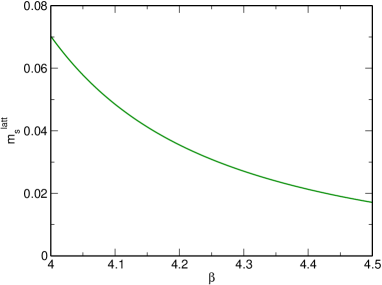
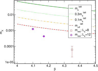
Using the parameterizations $a(\beta)$ and $Z_{m}(\beta)$ and the inputs Eq. (7) $m_{s}^{latt}(\beta)$ is determined and plotted in the left panel of Fig. 3. The right panel shows that with log-y scale, together with $m_{ud}^{latt}(\beta)$ determined from $m_{s}^{latt}(\beta)$ with Eq. (7), as well as $\alpha m_{s}^{latt}$ with $\alpha=0.3$ and $0.1$. The residual quark mass computed on the three ensembles are also shown.

Figure 3: Line of constant physics for $m_{s}^{latt}$ (left). Line of constant physics for $m_{s}^{latt}$, $0.3m_{s}^{latt}$, $0.1m_{s}^{latt}$ and $m_{ud}^{latt}$ in comparison with the residual quark mass (right).

3 Early results

In this section some early and preliminary results are shown. We use the scale setting and line of constant physics obtained in the previous section to simulate finite temperature QCD with fixed quark masses in physical unit and with varying temperature.

We adopt temporal size $N_{t}=12$ and $16$. The temperature - $\beta$ trajectories of interest are shown in Fig. 4.

Figure 4: Temperature as a function of $\beta$ for different temporal lattice size $N_{t}$. Target $T-\beta$ trajectories are shown as T1 for $N_{t}=12$ and T2 for $N_{t}=16$. Expected transition regions are marked as (a), (c) for $m_{l}=0.1m_{s}$, and (b) for physical $ud$ quark mass.

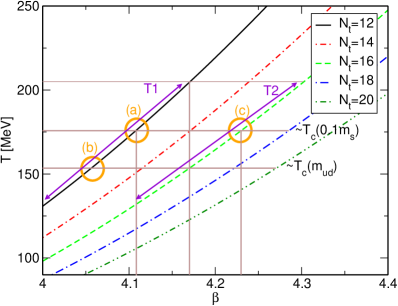
The strange quark mass is always tuned as physical (Eq. (7)). The simulated average $ud$ quark mass is set as one tenth of the strange for the moment ($m_{l}=m_{s}/10$). Note that for now we neglect the effect of $m_{res}$. The effect will be larger for coarser lattices and for smaller quark masses with a fixed $L_{s}$.

Figure 5 shows the variance of the iteration count of conjugate gradient for the light quark solver in the hybrid Monte Carlo simulations at $N_{t}=12$. As a first step we have chosen rather small aspect ratio of spatial and temporal lattice sizes as $N_{s}/N_{t}=2$. It develops a peak around $T\simeq 170$ MeV, which turns out to be consistent with the observation in a pilot study with fixed $\beta=4.17$ and varying $m_{l}$. This quantity may be used as an indicator of the transition as it should have a correlation with the fluctuation of physical quantities. It is useful in pinning down the transition region prior to performing various measurements on the configurations.

Figure 5: Variance of the iteration count of conjugate gradient for the light quark solver in the molecular dynamics at $N_{t}=12$ as a function of temperature.

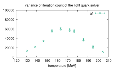
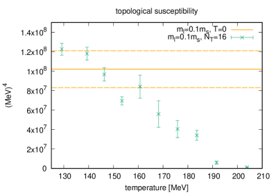
Figure 6 plots the topological susceptibility at $N_{t}=16$ computed using a gluonic definition with a cooling using the Wilson flow. Horizontal lines indicate the central value and error in the zero temperature [16]. At the low temperature region in this figure the $m_{res}$ effect is getting sizable as this quantity is sensitive to the change of the quark mass. The correction due to the $m_{res}$ effect is important in this region, which is yet to be determined.

Figure 6: Topological susceptibility as a function of temperature for $N_{t}=16$ and with the line of constant physics, $m_{l}=m_{s}/10$.

4 Summary and Outlook

In this article a status report was provided on the systematic investigation of the $2+1$-flavor finite-temperature QCD transition using Möbius domain-wall fermions at fine lattices up to $N_{t}=16$. The line of constant physics has been determined, with which a series of simulations have been performed aiming to get physics at the $ud$ quark mass being one tenth of the strange ((a) and (c) regions in Fig. 4). Various measurements of the fermionic observables are now underway, which will be used to determine the (pseudo) critical point and related physics around that. Understanding the size of $m_{res}$ around $\beta=4$, which is the lower edge of our finite temperature simulations, and its correction to the physical quantities are important especially for the coarser lattice ($N_{t}=12$). With that further study with lowering the light quark mass will be sought, using on-going simulations in the range (b) in Fig. 4.

References

- [1] O. Philipsen, Constraining the phase diagram of QCD at finite temperature and density, PoS LATTICE2019 (2019) 273 [1912.04827].
- [2] J. Guenther, An overview of the QCD phase diagram at finite and , these proceedings (Plenary talk presented in Lattice 2021) .
- [3] A. Lahiri, Aspects of finite temperature QCD approaching the chiral limit, these proceedings (Plenary talk presented in Lattice 2021) .
- [4] HotQCD collaboration, The chiral transition and symmetry restoration from lattice QCD using Domain Wall Fermions, Phys. Rev. D86 (2012) 094503 [1205.3535].
- [5] A. Tomiya, G. Cossu, S. Aoki, H. Fukaya, S. Hashimoto, T. Kaneko et al., Evidence of effective axial U(1) symmetry restoration at high temperature QCD, Phys. Rev. D96 (2017) 034509 [1612.01908].
- [6] JLQCD collaboration, Study of the axial anomaly at high temperature with lattice chiral fermions, Phys. Rev. D 103 (2021) 074506 [2011.01499].
- [7] JLQCD collaboration, Role of axial U(1) anomaly in chiral susceptibility of QCD at high temperature, 2103.05954.
- [8] R.D. Pisarski and F. Wilczek, Remarks on the chiral phase transition in chromodynamics, Phys. Rev. D29 (1984) 338.
- [9] R.C. Brower, H. Neff and K. Orginos, The Möbius domain wall fermion algorithm, Comput. Phys. Commun. 220 (2017) 1 [1206.5214].
- [10] K. Suzuki et al., Axial U(1) symmetry at high temperatures in lattice QCD with chiral fermions, these proceedings (Parallel talk presented in Lattice 2021) .
- [11] R.G. Edwards, U.M. Heller and T.R. Klassen, Accurate scale determinations for the wilson gauge action, Nucl. Phys. B517 (1998) 377 [hep-lat/9711003].
- [12] Flavour Lattice Averaging Group collaboration, FLAG Review 2019: Flavour Lattice Averaging Group (FLAG), Eur. Phys. J. C 80 (2020) 113 [1902.08191].
- [13] JLQCD collaboration, Renormalization of domain-wall bilinear operators with short-distance current correlators, Phys. Rev. D 94 (2016) 054504 [1604.08702].
- [14] K.G. Chetyrkin and A. Retey, Renormalization and running of quark mass and field in the regularization invariant and ms-bar schemes at three and four loops, Nucl. Phys. B583 (2000) 3 [hep-ph/9910332].
- [15] B. Colquhoun et al., Supplementary material in "Form factors of and determination of with Möbius domain-wall fermions", in preparation (2021) .
- [16] JLQCD collaboration, Topological susceptibility of QCD with dynamical Möbius domain-wall fermions, PTEP 2018 (2018) 043B07 [1705.10906].
- [17] N. Meyer, D. Pleiter, S. Solbrig and T. Wettig, Lattice QCD on upcoming Arm architectures, PoS LATTICE2018 (2019) 316 [1904.03927].