Instanton effects vs resurgence in the $O(3)$ sigma model

Abstract

We investigate the ground-state energy of the integrable two dimensional $O(3)$ sigma model in a magnetic field. By determining a large number of perturbative coefficients we explore the closest singularities of the corresponding Borel function. We then confront its median resummation to the high precision numerical solution of the exact integral equation and observe that the leading exponentially suppressed contribution is not related to the asymptotics of the perturbative coefficients. By analytically expanding the integral equation we calculate the leading non-perturbative contributions up to fourth order and find complete agreement. These anomalous terms could be attributed to instantons, while the asymptotics of the perturbative coefficients seems to be related to renormalons.

1 Introduction

Perturbation theory in quantum field theories is typically asymptotic with factorially growing coefficients. This factorial growth can be attributed to the proliferation of Feynman diagrams [1, 2] related to instantons, or to integrals in specific so called renormalon diagrams, when the loop momenta lie in various IR and UV domains [3]. Instantons correspond to non-trivial saddle points in the path integral, while renormalons do not have such a direct semiclassical interpretation. They both lead to non-perturbative contributions, exponentially suppressed in perturbation theory, which can typically be extracted from the large-order behaviour of the perturbative coefficients. The theory which describes this connection is known as resurgence theory see [4, 5, 6, 7] and references therein. In its strong version it states that all non-perturbative corrections have their seeds in the perturbative growths. In the present letter we would like to investigate a counter-example to this behaviour: the two dimensional $O(3)$ sigma model.

The two-dimensional $O(N)$ sigma models are ideal testing grounds for non-perturbative physics as they exhibit interesting physical phenomena including dynamical mass generation and asymptotic freedom, while they are integrable enabling the exact determination of their mass gap, scattering matrices, and the ground state energy in a magnetic field [8, 9, 10]. The $O(3)$ model is exceptional among the other $O(N)$ models as it is the only one having instantons [11].

The $O(N)$ models always played a pioneering role in the integrable investigations: starting from the exact calculation of the scattering matrix [8] to the exact determination of the mass gap [10, 9]. This mass gap was obtained by calculating the groundstate energy in a magnetic field through perturbation theory and by matching it to the expansion of the Wiener-Hopf solution of its exact integral equation. Volin’s method allowed to calculate many terms in this expansion whose factorial asymptotic behaviour revealed the leading singularities on the Borel plane [12, 13, 14]. A precision analysis in the $O(4)$ model showed non-trivial resurgence relations for the leading non-perturbative behaviour and allowed us to construct the first few terms in the ambiguity free trans-series, whose median resummation was in complete agreement with the numerical solution of the integral equation [15, 16]. Some of these analyses was put on analytical grounds in [17]. There were also analytical developments for large $N$ in [18, 19]. Recently the authors of [20] developed a technique to calculate the exponentially suppressed corrections systematically and observed anomalous terms for the $O(3)$ model.

The aim of our present paper is to repeat the analysis we did for the $O(4)$ model and compare the numerical solution of the integral equation to the median resummation of the trans-series built from the asymptotics of the perturbative expansion. As we also observe these anomalous terms we calculate their expansion beyond the results of [20] and match them to our numerical solution obtaining complete agreement.

The paper is organized as follows: In the next section we introduce the integrable description of the ground state energy in the $O(3)$ model, together with Volin’s approach, which leads to its perturbative expansion. Section 3 contains our numerical results. We first solve Volin’s equation numerically and determine the first 336 perturbative coefficients. Their asymptotic behaviour determines the closest singularities on the Borel plane, which we can characterize analytically. We then calculate the lateral Borel resummation of the perturbative series using the conformal Padé approximation. We subtract the real part of this result from a high precision solution of the exact integral equation and investigate the leading exponentially suppressed contributions. Surprisingly the leading, exponentially small deviation is not related to the asymptotics of the perturbative coefficients. In section 4 we perform an analytical expansion of the integral equation and determine the first few non-perturbative terms, which completely agrees with our numerical results. Finally we conclude in section 5.

2 O(3) sigma model

The $O(3)$ sigma model is an integrable two dimensional quantum field theory, consisting of three particles of mass $m$, whose non-diagonal scattering matrix is exactly known. By introducing a large enough magnetic field coupled to one of the $O(3)$ charges one type of particles can be forced to condense into the vacuum [9, 10]. The rapidity density of the vacuum condensate satisfies the following integral equation

$$\chi(B,\theta)-\int_{-B}^{B}\frac{d\theta^{\prime}}{2\pi}K(\theta-\theta^{\prime})\chi(B,\theta^{\prime})=\cosh\theta\quad,$$ (1)

where the kernel is the logarithmic derivative of the condensed particles’ scattering matrix, which takes a very simple form $K(\theta)=2\pi/(\theta^{2}+\pi^{2})$. The particle density and the energy density can be obtained from the rapidity density as

$$\rho(B)=m\int_{-B}^{B}\frac{d\theta}{2\pi}\chi(B,\theta)\quad;\qquad\epsilon(B)=m^{2}\int_{-B}^{B}\frac{d\theta}{2\pi}\cosh\theta\,\chi(B,\theta)\quad.$$ (2)

The parameter $B$ is related to the magnetic field and a large magnetic field $h$ corresponds to a large $B$. In order to make contact with ordinary perturbation theory it is customary to analyze $\epsilon/\rho^{2}$ as the function of the running coupling $\alpha$ which in the $O(3)$ model is defined by

$$\frac{1}{\alpha}=\ln\frac{m}{\Lambda}+\ln\frac{2\pi\rho}{m}=B+\frac{1}{2}\ln B+\ln 4-\frac{1}{2}+\ln\hat{\rho}\quad,$$ (3)

where $\Lambda$ is the perturbative scale [9], $\rho=\frac{\sqrt{B}}{\pi}Am\hat{\rho}$ and $A=e^{B+1/2}/4$.

In order to develop a perturbative expansion Volin [12, 13] investigated the resolvent $R(\theta)=\int_{-B}^{B}d\theta^{\prime}\,\frac{\chi(\theta^{\prime})}{\theta-\theta^{\prime}}$ and its Laplace transform $\hat{R}(s)=\int_{-i\infty+0}^{i\infty+0}\frac{dz}{2\pi i}e^{sz}R(B+z/2)$, where $z=2(\theta-B)$. Comparing their two alternative parametrizations

$$R(\theta)=\frac{2A\sqrt{B}}{\theta\sqrt{1-\frac{B^{2}}{\theta^{2}}}}\sum_{n,m=0}^{\infty}\sum_{k=0}^{n+m}\frac{c_{n,m,k}\left(\frac{\theta}{B}\right)^{p(k)}}{B^{m-n}(\theta^{2}-B^{2})^{n}}\left[\log\frac{\theta-B}{\theta+B}\right]^{k}\quad,$$ (4)

where $p(k)=k\,\mathrm{mod}\,2$ and

$$\hat{R}(s)=\frac{A}{\sqrt{s}}e^{-s\log(4s/e)}\frac{\Gamma(1+2s)}{\Gamma(\frac{1}{2}+s)}\left(\frac{1}{s+\frac{1}{2}}+\frac{1}{Bs}\sum_{n,m=0}^{\infty}\frac{Q_{n,m}}{B^{m+n}s^{n}}\right)\quad,$$ (5)

both the coefficients $c_{n,m,k}$ and $Q_{n,m}$ can be determined recursively. Once they are known the energy density is $\epsilon/m^{2}=e^{B}\hat{R}(1/2)/(4\pi)$, while the density is the residue of $R(\theta)$ at infinity. The first few perturbative orders are

$$\hat{\rho}=1+\frac{\ln 4+\frac{1}{2}\ln B-\frac{3}{4}}{2B}+O(1/B^{2})$$ (6)

and

$$\epsilon(B)=\frac{m^{2}e^{2B+1}}{16\pi}\,\hat{\epsilon}(B)\quad;\quad\hat{\epsilon}(B)=1+\frac{1}{4B}+O(1/B^{2})\quad.$$ (7)

Using the definition of $\alpha$ in (3) allows to calculate the perturbative expansion of

$$\frac{\epsilon}{\pi\rho^{2}}=\alpha+\frac{\alpha^{2}}{2}+\frac{\alpha^{3}}{2}+\dots=\sum_{n=1}^{\infty}\chi_{n}\alpha^{n}\quad.$$ (8)

3 Numerical investigations

By expanding $R(z)$ in powers of $z$ and performing the Laplace transform a double series in $s$ and $t=\log(4Bs)$ is obtained containing $c_{n,m,k}$. On the other hand $\hat{R}(s)$ can be also expanded similarly and matching the coefficients provides algebraic equations which can be solved recursively for the $c_{n,m,k}$ and $Q_{n,m}$ coefficients. At each step one can express the $c$ and $Q$ coefficients in terms of their smaller index counterparts. As the expressions containing zeta numbers, $\log(2)$ and $\gamma_{E}$ are growing very fast, it is not possible to go high orders with any reasonable computer resources. Even taking into account that $\log(2)$ , $\gamma_{E}$ and even $\zeta$ numbers eventually cancel we could not go over 50 coefficients. We then started to determine the coefficients numerically with a few thousand digits precision. With this approach we could reach 336 perturbative coefficients in more than a month of computer time. In the following we analyze these numerical coefficients.

The coefficients $\chi_{n}$ grow factorially such that

$$c_{n}=\chi_{n}2^{n-1}/\Gamma(n)$$ (9)

show constant asymptotics. The poles of the Padé approximant of $B(s)=\sum_{n=1}^{336}c_{n}s^{n-1}$ is demonstrated on Figure 1.

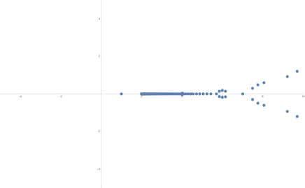
Figure 1: Poles of the Padé approximant on the Borel plane.

The Padé approximant clearly shows a pole singularity at $1$, a cut starting at $2$, possibly another cut starting at $4$ and may be more cuts on the positive real lines. It is clear that there is no singularity on the negative real line in contrast to the $O(N)$ models for $N>3$, see [12, 13, 14, 20]. Far from the origin our data are not precise enough as we observe spurious imaginary poles, which change their positions when we vary the nature or the order of the Padé approximant.

By using high order Richardson transform we can easily extract the large order behaviour of the $c_{n}$ coefficients

$$c_{n}=\frac{8}{e^{2}}+O(2^{-n})\quad.$$ (10)

We could see this on the 55th Richardson transform with a 98 digits precision. We then analysed with similar methods the subleading behaviour

$$(c_{n}-\frac{8}{e^{2}})\frac{2^{n-1}}{n}=a_{0}+\frac{a_{1}}{n}+\frac{a_{2}}{n(n-1)}+\dots\frac{a_{k}}{n(n-1)\dots(n-k+1)}+\dots$$ (11)

and found for 50 digits that

$$a_{0}=-\frac{32}{\pi e^{4}}\quad;\qquad\frac{a_{1}}{a_{0}}=-\frac{3}{2}\quad;\qquad\frac{a_{2}}{a_{0}}=\frac{1}{8}\quad.$$ (12)

Similarly we found

$$\frac{a_{3}}{a_{0}}=-\frac{127}{16}+6\zeta(3)\quad;\quad\frac{a_{4}}{a_{0}}=-\frac{35087}{384}+\frac{137\zeta(3)}{2}$$ (13)

$$\frac{a_{5}}{a_{0}}=\frac{1005\zeta(3)}{2}+\frac{405\zeta(5)}{2}-\frac{226801}{256}$$ (14)

with decreasing precisions. We also calculated the next 20 coefficients numerically and from the numerics we could observe that they behave as

$$a_{n}/a_{0}=\Gamma(n+2)(b_{0}+\frac{b_{1}}{n}+\dots)\quad,$$ (15)

but we could calculate the $b_{n}$ coefficients for $n=0,1,$ only with a few digits precision. $b_{0}$ seems to be $\frac{32}{\pi e^{4}}$ with 3 digits while $b_{1}/b_{0}\sim 5/2$ with two digits.

We then decided to compare the lateral Borel resummations of our perturbative answer to the numerical solution of the TBA equation. In the first step we elaborated on the numerical evaluation of the inverse Borel transform. If we had just used the Padé approximant of the perturbative series we would have faced the complex singularities (see Figure 1) on any ray of integrations. So we decided to use the conformal mapping $s=4w/(1+w)^{2}$ to rewrite the series on the Borel plane in powers of $w$. Technically we worked with

$$f(\alpha)=\frac{\epsilon}{\pi\rho^{2}}=\sum_{n=1}^{336}\chi_{n}\alpha^{n}\quad;\qquad B(s)=\sum_{n=0}^{335}c_{n+1}s^{n}\quad.$$ (16)

By using the conformal mapping we can calculate the $d_{n}$ coefficients from

$$B(s)=\sum_{n}d_{n}w(s)^{n}\quad;\qquad w(s)=\frac{1-\sqrt{1-s}}{1+\sqrt{1-s}}$$ (17)

by matching their perturbative $s$-expansions. We then can integrate

$$f_{+}(\alpha)=2\int_{0}^{e^{i/2}\infty}\sum_{n}d_{n}w(s)^{n}e^{-2s/\alpha}ds\quad.$$ (18)

We could even make a Padé approximation for $B(w)$ but it did not really change the result of the integral which we calculated at least for 50 digits.

We then solved the integral equation with a very high precision similar to [16]. This was done by expanding $\chi$ in a Chebisev basis on the interval $[-B,B]$. Due to the rational nature of the kernel we could calculate its matrix elements analytically and by inverting the matrix equation we calculated the representative of $\chi$. We managed to get $f_{\mathrm{TBA}}=\frac{\epsilon}{\pi\rho^{2}}$ as a function of $\alpha$ with 70 digits precision (in the worst case). We then compared $f_{\mathrm{TBA}}$ to $f_{+}$ separately for the imaginary and for the real part. The imaginary part started as

$$\Im m(f_{+})=\frac{16\pi}{e^{2}}e^{-2/\alpha}+\frac{e^{-4/\alpha}}{\alpha}\sum_{n=0}\tilde{a}_{n}\alpha^{n}\quad,$$ (19)

where we found that $\tilde{a}_{n}=\pi a_{n}4^{2-n}$ for $n=0,\dots,5$ with decreasing but at least 5 digits precision. Median resummation similar to [16] would suggest the form of the real deviation

$$f_{\mathrm{TBA}}-\Re e(f_{+})\propto e^{-8/\alpha}(4b_{0}+b_{1}\alpha+\dots)\quad,$$ (20)

however we observed a deviation of a much earlier order of the form

$$f_{\mathrm{TBA}}-\Re e(f_{+})=e^{-2/\alpha}A_{0}(2/\alpha+A_{1}+A_{2}\log\alpha+\alpha A_{3}+O(\alpha^{2}))\quad.$$ (21)

Originally we tried to fit a polynomial in $\alpha$ and failed to get a reasonable precision. In the recent paper [20] the authors calculated the leading coefficients to be

$$A_{0}=\frac{32}{e^{2}}\quad;\quad A_{1}=3-\gamma_{E}-5\log 2\quad;\quad A_{2}=1\quad.$$ (22)

By subtracting these coefficients we could fit $A_{3}=\frac{1}{2}$ with 5 digits and observed that there are no logarithmic correction at this order.

In order to test this prediction we expanded the integral equation one order higher than [20] and showed that indeed the only correction at this order is $A_{3}=\frac{1}{2}$. We summarize the details of the calculation in the next section.

4 Leading exponential corrections from the integral equation

The integral equation can be solved using the Wiener-Hopf technique. Here we summarize our results, while the details of the calculation will be given elsewhere. The idea of the calculation is to use Fourier transformation. If the integral went for the whole line we could easily calculate the Fourier transform of the kernel $\tilde{K}(\omega)=\int d\theta K(\theta)e^{i\omega\theta}$ and act with the inverse of $1-\tilde{K}(\omega)$ on the source

$$g(\omega)=\frac{e^{B}}{2i}\left(\frac{e^{iB\omega}}{\omega-i}-\frac{e^{-iB\omega}}{\omega+i}\right)+\frac{e^{-B}}{2i}\left(\frac{e^{iB\omega}}{\omega+i}-\frac{e^{-iB\omega}}{\omega-i}\right)\quad.$$ (23)

Since $\chi(B,\theta)$ is non-vanishing only on the interval $[-B,B]$ the integral equation is not satisfied for $|\theta|>B$. In the Wiener-Hopf technique we introduce the missing function and determine it by separating the equations in Fourier space into terms analytic on the lower and upper half planes, see [20] for the details in the present context. This requires to find the factorization

$$(1-\tilde{K}(\omega))^{-1}=G_{+}(\omega)G_{-}(\omega)\quad,$$ (24)

where $G_{+}(\omega)$, $G_{-}(\omega)=G_{+}(-\omega)$ are analytic on the upper/lower half plane. We also need integral operators $f(\omega)_{\pm}=\pm\frac{i}{2\pi}\int_{-\infty}^{\infty}\frac{f(\omega^{\prime})d\omega^{\prime}}{\omega-\omega^{\prime}\pm i0}$ to project on the corresponding components. This integral contour then can be deformed to surround the singularities of $G_{-}(\omega)$ and $G_{-}(\omega)/G_{+}(\omega)$, which are on the positive imaginary line. The speciality of the $O(3)$ model is that

$$G_{-}(\omega)=\frac{(2e)^{\frac{i\omega}{2}}}{\sqrt{\pi}}(i\omega)^{\frac{1}{2}i(i-\omega)}\Gamma\left(1+\frac{i\omega}{2}\right)$$ (25)

is nonvanishing at $i$: $G_{-}(i)=1/\sqrt{2e}$ and the pole $1/(\omega-i)$ will contribute from the source term. This term will appear in the unknown function and also in the Fourier transform of $\chi$ which should be taken at $i$ to get the ground state energy.

After redefining some functions we need to solve the integral equations

$$q^{(\pm)}(x)+\frac{1}{\pi}\int_{{\cal C}_{+}}\frac{e^{-y}\beta(\frac{y}{4B})q^{(\pm)}(y)}{x+y}\,dy=\frac{1}{1\pm\frac{x}{2B}}\quad,$$ (26)

where $\beta(x)=i(G_{-}(2ix+0)-G_{-}(2ix-0))/2G_{+}(2ix)$ and the ${\cal C}_{+}$ integration goes from zero to infinity, avoiding the poles of the integrand at $y=4B,8B,\dots$ from the left. This contour is equivalent to the integration path chosen for the perturbative part in (18). From the solutions $q^{(\pm)}$ the leading exponential correction of $\hat{\epsilon}=\hat{\epsilon}_{\mathrm{pert}}+e^{-2B}\delta\hat{\epsilon}$ can be calculated via

$$u^{(\pm)}=\frac{1}{\pi}\int_{{\cal C}_{+}}\frac{e^{-y}\beta(\frac{y}{4B})q^{(\pm)}(y)}{2B\mp y}\,dy$$ (27)

as

$$\begin{split}\delta\hat{\epsilon}&=\frac{-i\pi}{e}+\frac{2}{e}[2B-\ln 2-\gamma_{E}+1-u^{(+)}-u^{(-)}]\\ &=\frac{-i\pi}{e}+\frac{2}{e}[2B-\ln 2-\gamma_{E}+1-\frac{1}{4B}+O(1/B^{2})]\quad.\end{split}$$ (28)

Although the density $\rho$ is related to the Fourier transform of $\chi$ at the origin, it is simpler to extract it from the solution of an integral equation similar to (1) but with a source term being $1$ instead of $\cosh\theta$. Repeating the calculation for $\hat{\rho}=\hat{\rho}_{\mathrm{pert}}+e^{-2B}\delta\hat{\rho}$ gives

$$\delta\hat{\rho}=-\frac{1}{e}\left\{1+\frac{\ln 4+\frac{1}{2}\ln B+\frac{3}{4}}{2B}+O(1/B^{2})\right\}\quad.$$ (29)

Due to this term the running coupling (3) acquires a non-perturbative correction, too. Thus the sought for quantity $\epsilon/\rho^{2}$ receives corrections from three sources. It gets corrections directly from (28) and from (29) and indirectly from the running coupling (3) leading finally to

$$\frac{\epsilon}{\pi\rho^{2}}=\alpha+\frac{\alpha^{2}}{2}+\dots+e^{-\frac{2}{\alpha}}\frac{32}{e^{2}}\left(-\frac{i\pi}{2}+\frac{2}{\alpha}+3-\gamma_{E}-5\log 2+\log\alpha+\frac{\alpha}{2}+\dots\right)+O(e^{-\frac{4}{\alpha}})\quad.$$ (30)

Here the asymptotic perturbative series is understood as Borel resummed by (18), thus the imaginary non-perturbative part from the integral nicely cancels with the similar term coming from the pole term. The $\alpha/2$ term in the bracket is our new result compared to [20]. We compare this newly calculated $\alpha/2$ term to the numerically determined $f_{\mathrm{TBA}}-\Re e(f_{+})$ on Figure 2 and find complete agreement. In the inset we plot the difference of these two, which signals that the next order terms are much smaller.

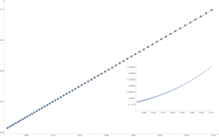
Figure 2: Comparison of the numerically determined $f_{\mathrm{TBA}}-\Re e(f_{+})$ to the analytically calculated new term $\alpha/2$. In particular $\Delta f=e^{2/\alpha}e^{2}/16(f_{\mathrm{TBA}}-\Re e(f_{+}))-2(2/\alpha+3-\gamma_{E}-5\log 2+\log\alpha)$ is plotted against $\alpha$ with dots, while the newly calculated $\alpha$ term with a continous line. The inset demonstrates the difference between the numerics and the new analytical term.

5 Conclusion

In this letter we investigated the groundstate energy of the $O(3)$ sigma model both numerically and analytically. On the numerical side we calculated the first 336 perturbative coefficients with very high precisions. Their asymptotic behaviour allowed us to map and characterize the closest singularities on the Borel plane: a single pole and a cut signaling imaginary ambiguities of the form $\tilde{a}e^{-2/\alpha}$ and $e^{-4/\alpha}/\alpha(\tilde{a}_{0}+\tilde{a}_{1}\alpha+\dots.$). We identified the appearing coefficients $\tilde{a}$ with high precision in terms of $16/e^{2}$ and odd zeta functions. We even investigated their asymptotics which contributes via the median resummation to the real part of the groundstate energy of order $e^{-8/\alpha}$, see [16] for a similar analysis in the $O(4)$ model. We then compared the median resummation of the perturbative and non-perturbative terms originating from the asymptotics of the perturbative series to the high precision solution of the integral equations and observed an anomalous $e^{-2/\alpha}$ deviation, which cannot be attributed in any way to the perturbative coefficients. We then, following [20], expanded analytically the integral equation and matched the results against the observed deviation and found complete agreement.

Our analytical calculation differs technically, but not conceptually from the calculation in [20] since we calculated $\epsilon/\rho^{2}$ as the function of $\rho(B)$, while they calculated the free energy as the function of the magnetic field. These quantities are related by a Legendre transformation. Furthermore, our calculation goes one order beyond the result of [20].

These results strongly indicate that the anomalous non-perturbative terms are not related to the asymptotics of the perturbative series. This is exceptional for the $O(3)$ model and does not appear for any higher $N$ [15, 16, 20, 18, 19]. Since the $O(3)$ model is the only one with instantons, we believe that the anomalous terms are related to the instantons, while the regular terms are related to renormalons. Indeed such terms for other $O(N)$ models in the large $N$ limit were matched to renormalon diagrams in perturbation theory [18, 19]. It would be extremely interesting to match the observed anomalous non-perturbative behaviour with explicit instanton calculations.

Acknowledgements

Our work was supported by ELKH, with infrastructure provided by the Hungarian Academy of Sciences. This work was supported by NKFIH grant K134946.

References

- [1] C. A. Hurst, The Enumeration of Graphs in the Feynman-Dyson Technique, Proc. Roy. Soc. Lond. A 214 (1952) 44. doi:10.1098/rspa.1952.0149.
- [2] L. Lipatov, Divergence of the Perturbation Theory Series and the Quasiclassical Theory, Sov. Phys. JETP 45 (1977) 216–223.
- [3] M. Beneke, Renormalons, Phys. Rept. 317 (1999) 1–142. arXiv:hep-ph/9807443, doi:10.1016/S0370-1573(98)00130-6.
- [4] D. Dorigoni, An Introduction to Resurgence, Trans-Series and Alien Calculus, Annals Phys. 409 (2019) 167914. arXiv:1411.3585, doi:10.1016/j.aop.2019.167914.
- [5] G. V. Dunne, M. Ünsal, What is QFT? Resurgent trans-series, Lefschetz thimbles, and new exact saddles, PoS LATTICE2015 (2016) 010. arXiv:1511.05977, doi:10.22323/1.251.0010.
- [6] I. Aniceto, G. Basar, R. Schiappa, A Primer on Resurgent Transseries and Their Asymptotics, Phys. Rept. 809 (2019) 1–135. arXiv:1802.10441, doi:10.1016/j.physrep.2019.02.003.
- [7] M. Mariño, Lectures on non-perturbative effects in large gauge theories, matrix models and strings, Fortsch. Phys. 62 (2014) 455–540. arXiv:1206.6272, doi:10.1002/prop.201400005.
- [8] A. B. Zamolodchikov, A. B. Zamolodchikov, Relativistic Factorized S Matrix in Two-Dimensions Having O(N) Isotopic Symmetry, JETP Lett. 26 (1977) 457. doi:10.1016/0550-3213(78)90239-0.
- [9] P. Hasenfratz, M. Maggiore, F. Niedermayer, The Exact mass gap of the O(3) and O(4) nonlinear sigma models in d = 2, Phys. Lett. B 245 (1990) 522–528. doi:10.1016/0370-2693(90)90685-Y.
- [10] P. Hasenfratz, F. Niedermayer, The Exact mass gap of the O(N) sigma model for arbitrary in d = 2, Phys. Lett. B 245 (1990) 529–532. doi:10.1016/0370-2693(90)90686-Z.
- [11] A. M. Polyakov, A. A. Belavin, Metastable States of Two-Dimensional Isotropic Ferromagnets, JETP Lett. 22 (1975) 245–248.
- [12] D. Volin, From the mass gap in O(N) to the non-Borel-summability in O(3) and O(4) sigma-models, Phys. Rev. D 81 (2010) 105008. arXiv:0904.2744, doi:10.1103/PhysRevD.81.105008.
- [13] D. Volin, Quantum integrability and functional equations: Applications to the spectral problem of AdS/CFT and two-dimensional sigma models, Ph.D. thesis (2009). arXiv:1003.4725, doi:10.1088/1751-8113/44/12/124003.
- [14] M. Mariño, T. Reis, Renormalons in integrable field theories, JHEP 04 (2020) 160. arXiv:1909.12134, doi:10.1007/JHEP04(2020)160.
- [15] M. C. Abbott, Z. Bajnok, J. Balog, A. Hegedűs, From perturbative to non-perturbative in the O(4) sigma model, Phys. Lett. B 818 (2021) 136369. arXiv:2011.09897, doi:10.1016/j.physletb.2021.136369.
- [16] M. C. Abbott, Z. Bajnok, J. Balog, A. Hegedűs, S. Sadeghian, Resurgence in the O(4) sigma model, JHEP 05 (2021) 253. arXiv:2011.12254, doi:10.1007/JHEP05(2021)253.
- [17] Z. Bajnok, J. Balog, I. Vona, Analytic resurgence in the O(4) model, arXiv:2111.15390.
- [18] M. Marino, R. Miravitllas, T. Reis, Testing the Bethe ansatz with large N renormalons (2 2021). arXiv:2102.03078, doi:10.1140/epjs/s11734-021-00252-4.
- [19] L. Di Pietro, M. Mariño, G. Sberveglieri, M. Serone, Resurgence and 1/N Expansion in Integrable Field Theories, JHEP 10 (2021) 166. arXiv:2108.02647, doi:10.1007/JHEP10(2021)166.
- [20] M. Marino, R. Miravitllas, T. Reis, New renormalons from analytic trans-series, arXiv:2111.11951.