D-HYPR: Harnessing Neighborhood Modeling and Asymmetry Preservation for Digraph Representation Learning

Abstract.

Digraph Representation Learning (DRL) aims to learn representations for directed homogeneous graphs (digraphs). Prior work in DRL is largely constrained (e.g., limited to directed acyclic graphs), or has poor generalizability across tasks (e.g., evaluated solely on one task). Most Graph Neural Networks (GNNs) exhibit poor performance on digraphs due to the neglect of modeling neighborhoods and preserving asymmetry. In this paper, we address these notable challenges by leveraging hyperbolic collaborative learning from multi-ordered and partitioned neighborhoods, and regularizers inspired by socio-psychological factors. Our resulting formalism, Digraph Hyperbolic Networks (D-HYPR) – albeit conceptually simple – generalizes to digraphs where cycles and non-transitive relations are common, and is applicable to multiple downstream tasks including node classification, link presence prediction, and link property prediction. In order to assess the effectiveness of D-HYPR, extensive evaluations were performed across $8$ real-world digraph datasets involving $21$ prior techniques. D-HYPR statistically significantly outperforms the current state of the art. We release our code at https://github.com/hongluzhou/dhypr

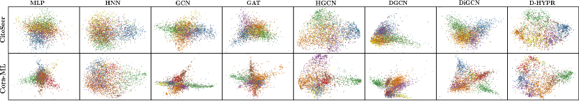
Figure 1. Embedding space visualization using PCA projection. Our method D-HYPR leads to the best class separation. Each dot represents a node, and colors reflect the ground truth class labels of nodes, which are best appreciated when zooming in.

1. Introduction

Directionality is a fundamental characteristic inherent in a multitude of real-world graphs, including social networks, web page networks, and citation networks (Ou et al., 2016). Digraph Representation Learning (DRL) aims to learn representations for directed homogeneous graphs (digraphs) (Tong et al., 2020a; Zhang et al., 2021a). Early DRL techniques include factorization-based approaches such as HOPE (Ou et al., 2016) and ATP (Sun et al., 2019), and random walk-based approaches such as APP (Zhou et al., 2017) and NERD (Khosla et al., 2019). However, these methods do not scale to large digraphs, or are sensitive to outliers and noise. In recent years, Graph Neural Networks (GNNs) have achieved immense success on a wide range of tasks (Zhou et al., 2020). However, GNNs primarily aim at representation learning for undirected graphs. There are two notable challenges that hinder their effectiveness on digraphs.

Challenge 1: Neighborhood Modeling. The neighborhoods of a node may possess unique semantics. For instance, in social networks, in-neighbors are commonly known as followers, while out-neighbors are accounts that the user follows. In citation networks, in-neighbors of a node can be existing works cited by a paper by the time the camera-ready version of the paper is submitted, whereas out-neighbor connections arise subsequent to the paper coming out. Existing GNN techniques (Kipf and Welling, 2016b; Veličković et al., 2017; Chami et al., 2019; Zhu et al., 2020) transform digraphs to undirected graphs to enable running experiments, which simplifies the learning problem, or only consider the direct out-neighbors in the graph convolution. Thus, they lose characteristics of the original structure, resulting in misleading message passing and ultimately subpar results on digraph-specific problems.

Challenge 2: Asymmetry Preservation. Due to the inherent symmetry of popular measures, such as the inner product or distance in the embedding space, which produces the same scores for the node pair $(i,j)$ and $(j,i)$, inner-product- or distance-based learning objectives used by popular GNNs are unsuitable for capturing the asymmetric connection probabilities for node pairs in digraphs (Salha et al., 2019). Applications based on link prediction or graph topology learning are particularly affected when models fail to preserve digraph structural asymmetry.

Recently, spectral-based DRL GNNs (Zhang et al., 2021a; Tong et al., 2020a, b; Ma et al., 2019b) have been proposed to address Challenge 1 with respect to modelling neighborhoods for digraphs. However, the learned filters from these methods depend on the Laplacian eigenbasis, which is tied to a graph's structure (Tong et al., 2021). Models trained on a specific structure cannot be directly applied to graphs with different structures (Wu et al., 2020). Separately, to address Challenge 2, approaches such as viewing directions of edges as a kind of edge feature (Gong and Cheng, 2019), or parametrizing the node pair likelihood function by a neural network (Shi et al., 2019; Battaglia et al., 2018) have been proposed, but these techniques fail to consider Challenge 1. Moreover, prior DRL techniques are often constrained to directed acyclic graphs (DAGs) (Thost and Chen, 2021; Ganea et al., 2018a; Suzuki et al., 2019), are transductive (Sim et al., 2021; Tong et al., 2020b; Ganea et al., 2018a; Suzuki et al., 2019), or have poor generalizability across tasks. For example, some studies provide experimental evidence for a single task only – e.g., link prediction as in (Sim et al., 2021) or node classification as in (Tong et al., 2020b; Ma et al., 2019b).

We propose Digraph HYPERbolic Networks (D-HYPR) to fully address these limitations. To overcome Challenge 1, D-HYPR utilizes hyperbolic collaborative learning from multi-ordered and partitioned neighborhoods. For Challenge 2, D-HYPR takes advantage of self-supervised learning, using asymmetry-preserving regularizers supported by well-established socio-psychological theories (McPherson et al., 2001; Mitzenmacher, 2004). Specifically:

1. Neighborhood Modeling with Partitioned and Larger Receptive Fields: by leveraging collaborative learning from multi-ordered four canonical types of neighborhoods (Fig. 2 (a)), D-HYPR models the distinct node neighborhoods, and captures the local directed graph characteristics.

2. Neighborhood Modeling with a non-Euclidean Space: D-HYPR learns node representations of real-world digraphs (which exhibit scale-free or hierarchical structures) in hyperbolic space to avoid distortion of node neighborhoods.

3. Asymmetry Preservation with Regularizers: motivated by two decomposed causes of link formation, homophily (McPherson et al., 2001) and preferential attachment (Mitzenmacher, 2004), we employ two regularizers in training D-HYPR, which are used in a self-supervised fashion to account for each of the two driving forces of link formation. These regularizers lead to performance gains in downstream tasks.

4. Flexibility due to Message-passing-based GNN Formalism: D-HYPR falls into the category of message-passing-based GNNs that capture both graph structure and semantics. D-HYPR has the capability to inductively learn representations for general digraphs that potentially contain cycles, non-transitive relations, outliers, and noise.

Our contributions are three-fold: (1) We propose D-HYPR for DRL. D-HYPR considers the unique node neighborhoods in digraphs with multi-scale neighborhood collaboration in hyperbolic space. D-HYPR respects asymmetric relationships of node-pairs, which is guided by sociopsychology-inspired regularizers. (2) We perform extensive benchmarking experiments across 8 real-world digraph datasets. Our evaluation involves 4 tasks and 21 prior methods. Results demonstrate the significant superiority of D-HYPR against the state of the art. (3) D-HYPR generates meaningful embeddings in very low dimensionalities. This added benefit is desirable for large-scale real-world applications by efficiently saving space while preserving effectiveness.

2. Related Work

Graph Representation Learning (GRL). GRL methods have evolved from matrix factorization (Jiang et al., 2016), graph kernels (Shervashidze et al., 2011), and random walk-based transductive models (Perozzi et al., 2014), into GNNs (Kipf and Welling, 2016a), which have greatly surpassed these prior methods in numerous experiments. Interested readers may refer to comprehensive reviews (Zhou et al., 2020; Cai et al., 2018; Kriege et al., 2020; Wu et al., 2020) for further details. Current popular GRL approaches (Beani et al., 2021; Kipf and Welling, 2016a; Veličković et al., 2017; Chami et al., 2019; Zhu et al., 2020; Zhang et al., 2021b; Beani et al., 2021) have primarily considered undirected homogeneous GRL. Although certain recent GNNs can be applied to digraphs, e.g., the Graphormer (Ying et al., 2021) with its Transformer-based design (Vaswani et al., 2017), these techniques have been validated solely by experiments on undirected graphs (Zhang et al., 2021a), and are computationally impractical for large-scale digraphs.

Directed Graph Embedding. There are comparatively few studies that address DRL. HOPE (Ou et al., 2016) captures asymmetric transitivity but depends on a low rank assumption of the input, and fails to generalize to a variety of tasks (Khosla et al., 2019). APP (Zhou et al., 2017) captures asymmetry by relying on random walks. ATP (Sun et al., 2019) removes cycles in digraphs beforehand and then leverages factorization. NERD (Khosla et al., 2019) extracts a source and a target walk, and employs a shallow neural model. DGCN (Tong et al., 2020b), DiGCN (Tong et al., 2020a) and MagNet (Zhang et al., 2021a) are recent GNNs that extend spectral-based GCNs (Kipf and Welling, 2016a) to digraphs, but are tied to a graph’s Laplacian. DAGNN (Thost and Chen, 2021) is proposed for DAGs by injecting a DAG-specific inductive bias—partial ordering—into the GNN design.

Hyperbolic Embedding Learning. Most non-Euclidean embedding techniques (Ganea et al., 2018b; Nickel and Kiela, 2017; Gu et al., 2018; Nickel and Kiela, 2018; Law and Stam, 2020; Sim et al., 2021) only account for the graph structure and do not leverage node features. In contrast, we consider the general DRL setting of seeking to capture both digraph structure and attributes, and propose a message-passing-based GNN with an inductive learning capability.

HGCN (Chami et al., 2019) and HGNN (Liu et al., 2019) were proposed concurrently to generalize GNNs to take advantage of the strength of hyperbolic geometries. Other hyperbolic GNNs include Constant Curvature GCNs (Bachmann et al., 2020) that provide a mathematically grounded generalization of GCNs, HAT (Zhang et al., 2021b) that studies hyperbolic GNN with an attention mechanism, GIN (Zhu et al., 2020) that draws on both Euclidean and hyperbolic geometries, and so on (Dai et al., 2021; Chen et al., 2021; Zhang et al., 2021c). Our work is built upon these prior efforts on hyperbolic GNNs for undirected graphs, to address challenges associated with digraphs.

3. Preliminaries

Definition 0.

Digraph Representation Learning (Tong et al., 2020a; Zhang et al., 2021a). Let $\mathcal{G}=(\mathcal{V},\mathcal{E})$ be a homogeneous graph with vertex set $\mathcal{V}$ and edge set $\mathcal{E}$. Each edge $e\in\mathcal{E}$ is an ordered pair $e=(i,j)$ between vertices $i$ and $j$. The adjacency matrix of $\mathcal{G}$ can be denoted as $A=\{0,1\}^{|\mathcal{V}|\times|\mathcal{V}|}$. $\mathcal{G}$ is a digraph when ${\exists}(i,j),A_{i,j}\neq A_{j,i}$.

Nodes are described by a feature matrix $X^{0,E}\in\mathbb{R}^{|\mathcal{V}|\times d}$, i.e., each node $i\in\mathcal{V}$ has a $d$-dimensional Euclidean feature $\mathbf{x}_{i}^{0,E}$. The superscript ^E indicates that the vector lies in a Euclidean space, while ^H denotes a hyperbolic vector. $0$ denotes the input layer.

DRL is an effective and efficient solution for digraph analytics. The efficiency is achieved by converting the adjacency-matrix-based data into low-dimensional embeddings. Thus, the goal of DRL is to learn a mapping

(1) $$\small f:\left(\mathcal{V},\mathcal{E},\left(\mathbf{x}_{i}^{0,E}\right)_{i\in\mathcal{V}}\right)\rightarrow Z\in\mathbb{R}^{|\mathcal{V}|\times d^{\prime}}\vspace{-3pt}$$

that maps nodes to low-dimensional ($d^{\prime}\ll|\mathcal{V}|$) embedding vectors. These should capture both structural and semantic information and be valuable for downstream tasks.

Definition 0.

The Poincaré Ball Model. The Poincaré ball model (Ganea et al., 2018b) $\left(\mathbb{D}_{c}^{n},g^{c}\right)$ is defined by the $n$-dimensional manifold $\mathbb{D}_{c}^{n}=\{x\in\mathbb{R}^{n}:$ $c\left\lVert\mathbf{x}\right\rVert<1\}$ equipped with the Riemannian metric: $g_{\mathbf{x}}^{c}=\lambda_{\mathbf{x}}^{2}g^{E}$, where $\lambda_{\mathbf{x}}:=\frac{2}{1-c\left\lVert\mathbf{x}\right\rVert^{2}}$, $g^{E}=\mathbf{I}_{n}$ is the Euclidean metric tensor, and $c>0$ (we refer to $-c$ as the curvature). $\mathbb{D}_{c}^{n}$ is the open ball of radius $1/\sqrt{c}$. The connections between hyperbolic space and tangent space are established by the exponential map $\exp_{\mathbf{x}}^{c}:\mathcal{T}_{\mathbf{x}}\mathbb{D}_{c}^{n}\rightarrow\mathbb{D}_{c}^{n}$ and logarithmic map $\log_{\mathbf{x}}^{c}:\mathbb{D}_{c}^{n}\rightarrow\mathcal{T}_{\mathbf{x}}\mathbb{D}_{c}^{n}$:

(2) $$\small\exp_{\mathbf{x}}^{c}(\mathbf{v})=\mathbf{x}\oplus_{c}\left(\tanh\left(\sqrt{c}\frac{\lambda_{\mathbf{x}}^{c}\left\lVert\mathbf{v}\right\rVert}{2}\right)\frac{\mathbf{v}}{\sqrt{c}\left\lVert\mathbf{v}\right\rVert}\right)$$

(3) $$\small\log_{\mathbf{x}}^{c}(\mathbf{y})=\frac{2}{\sqrt{c}\lambda_{\mathbf{x}}^{c}}\tanh^{-1}\left(\sqrt{c}\left\lVert-\mathbf{x}\oplus_{c}\mathbf{y}\right\rVert\right)\frac{-\mathbf{x}\oplus_{c}\mathbf{y}}{\left\lVert-\mathbf{x}\oplus_{c}\mathbf{y}\right\rVert}$$

where $\mathbf{x},\mathbf{y}\in\mathbb{D}_{c}^{n}$, $\mathbf{v}\in\mathcal{T}_{\mathbf{x}}\mathbb{D}_{c}^{n}$, and $\oplus_{c}$ denotes Möbius addition, and

(4) $$\small\mathbf{x}\oplus_{c}\mathbf{y}:=\frac{\left(1+2c\langle\mathbf{x},\mathbf{y}\rangle+c\left\lVert\mathbf{y}\right\rVert^{2}\right)\mathbf{x}+\left(1-c\left\lVert\mathbf{x}\right\rVert^{2}\right)\mathbf{y}}{1+2c\langle\mathbf{x},\mathbf{y}\rangle+c^{2}\left\lVert\mathbf{x}\right\rVert^{2}\left\lVert\mathbf{y}\right\rVert^{2}}.$$

The Möbius scalar multiplication (Eq. 5) and Möbius matrix multiplication of $\mathbf{x}\in\mathbb{D}_{c}^{n}\backslash\{\mathbf{0}\}$ (Eq. 6) are

(5) $$\small r\otimes_{c}\mathbf{x}:=\frac{1}{\sqrt{c}}\tanh\left(r\tanh^{-1}(\sqrt{c}\left\lVert\mathbf{x}\right\rVert)\right)\frac{\mathbf{x}}{\left\lVert\mathbf{x}\right\rVert}$$

(6) $$M\otimes_{c}\mathbf{x}:=(1/\sqrt{c})\tanh\left(\frac{\left\lVert M\mathbf{x}\right\rVert}{\left\lVert\mathbf{x}\right\rVert}\tanh^{-1}(\sqrt{c}\left\lVert\mathbf{x}\right\rVert)\right)\frac{M\mathbf{x}}{\left\lVert M\mathbf{x}\right\rVert}$$

where $r\in\mathbb{R}$ and $M\in\mathbb{R}^{m\times n}$. The induced distance function on $\left(\mathbb{D}_{c}^{n},g^{c}\right)$ is given by

(7) $$\small d_{\mathbb{D}_{c}^{n}}(\mathbf{x},\mathbf{y})=(2/\sqrt{c})\tanh^{-1}\left(\sqrt{c}\left\lVert\mathbf{-x}\oplus_{c}\mathbf{y}\right\rVert\right)$$

For a longer introduction of hyperbolic or non-Euclidean geometry, we refer readers to relevant previous work (Bronstein et al., 2017; Chamberlain et al., 2017; Ganea et al., 2018b; Chami et al., 2019; Sala et al., 2018).

4. Methodology

Driven by the goal of addressing the challenge of Neighborhood Modeling and Asymmetry Preservation in digraphs, we propose D-HYPR (Fig. 2 (b)), which leverages hyperbolic collaborative learning from multi-ordered and partitioned neighborhoods, and self-supervised learning via asymmetry-preserving regularizers.

Euclidean space does not provide the most powerful or meaningful geometrical representations when input data exhibits a highly complex non-Euclidean latent anatomy, as for instance for real-world digraphs with a scale-free or hierarchical structure (Bronstein et al., 2017; Chamberlain et al., 2017). As the volume of nodes grows exponentially with the distance from a central node, non-Euclidean geometry is more suitable than Euclidean for embedding such digraphs (Sala et al., 2018; Sim et al., 2021; Law and Stam, 2020). Hyperbolic embeddings can incur smaller data distortion for real-world digraphs, which leads to a better representation of the nodes' local neighborhoods. This motivates our investigation of utilizing hyperbolic GNNs over Euclidean counterparts as the backbone for DRL.

4.1. Hyperbolic Embedding Learning

To perform message passing in hyperbolic space, the general efficient approach is to move basic operations of hyperbolic space to the tangent space (Zhang et al., 2021b; Zhu et al., 2020). Given $\mathcal{G}$ and $\mathbf{x}_{i}^{0,E}$, we first obtain $\mathbf{x}_{i}^{0,H}$ by applying exponential map $\exp_{\mathbf{0}}^{c^{0}}(\cdot)$ to map the Euclidean input feature $\mathbf{x}_{i}^{0,E}$ into hyperbolic space with curvature $-c^{0}\in\mathbb{R}$, where $c^{0}$ is learned in training. Hyperbolic message passing (Eqs. 8 to 10) is then performed by multiple layers (forming the Hyperbolic Graph Embedding Layers in Fig. 2 (b)). The layer is indexed by $\ell$, ranging from $1$ to a pre-defined integer $l$.

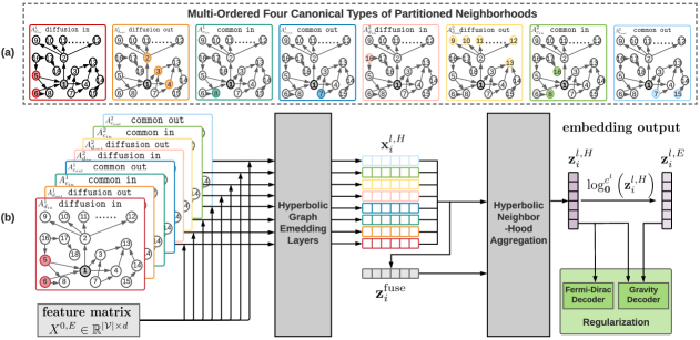
Figure 2. (a) Multi-ordered and partitioned neighborhoods. We define four types of $k$-order proximity matrix (shown in the figure with $k=1,2$ with respect to node $1$) to incorporate the pertinent subsets of neighbors and multi-scale information. (b) Methodology overview. D-HYPR learns a node representation from each neighborhood in hyperbolic space with Hyperbolic Graph Embedding Layers. Hyperbolic Neighborhood Aggregation further enables a closer collaboration of neighborhoods. D-HYPR respects asymmetric relationships of nodes with the hyperbolic Fermi-Dirac and Gravity regularizers.

(1) Hyperbolic Feature Transformation is performed by

(8) $$\small\mathbf{m}_{i}^{\ell,H}=W^{\ell}\otimes_{c^{\ell-1}}\mathbf{x}_{i}^{\ell-1,H}\oplus_{c^{\ell-1}}\mathbf{b},$$

where $W^{\ell}\in\mathbb{R}^{F^{\ell}\times F^{\ell-1}}$ is the weight matrix, and $\mathbf{b}\in\mathbb{D}_{c^{\ell-1}}^{F^{\ell}}$ denotes the bias (both are learned). We employ a unique trainable curvature at each layer to obtain a suitable hyperbolic space to account for different depths of the neural network.

(2) Hyperbolic Neighbor Aggregation. We then leverage the bridging between the hyperbolic space and the tangent space to perform neighbor aggregation (Zhang et al., 2021b; Zhu et al., 2020), resulting in $\mathbf{h}_{i}^{\ell,H}\in\mathbb{D}_{c^{\ell-1}}^{F^{\ell}}$,

(9) $$\small\mathbf{h}_{i}^{\ell,H}=\exp_{\mathbf{0}}^{c^{\ell-1}}\left(\sum_{j\in\{i\}\cup\mathcal{N}(i)}e_{ij}\log_{\mathbf{0}}^{c^{\ell-1}}\left(\mathbf{m}_{j}^{\ell,H}\right)\right).$$

$\mathcal{N}(i)=\{j:(i,j)\in\mathcal{E}\}$ denotes the set of neighbors of $i\in\mathcal{V}$. We apply out-degree normalization of $A$ (adjacency matrix), i.e., $D_{\text{out }}^{-1}(A+I)$, to obtain the aggregation weights for simplicity (while $e_{ij}$ can be computed with different mechanisms such as attention or leveraging edge attributes if present). $D_{\text{out }}$ is a diagonal matrix such that element $(i,i)$ is the sum of row $i$ in $A$ plus $1$. We choose the tangent space of the origin for efficiency (Chami et al., 2019).

(3) Non-Linear Activation with Trainable Curvatures. $\mathbf{x}_{i}^{\ell,H}\in\mathbb{D}_{c^{\ell}}^{F^{\ell}}$, the output hyperbolic representation of node $i$ in layer $\ell$ is set as

(10) $$\small\mathbf{x}_{i}^{\ell,H}=\exp_{\mathbf{0}}^{c^{\ell}}\left(\sigma\left(\log_{\mathbf{0}}^{c^{\ell-1}}\left(\mathbf{h}_{i}^{\ell,H}\right)\right)\right).$$

To smoothly vary the curvature of each layer, in Eq. 10, we first map $\mathbf{h}_{i}^{\ell,H}$ to the tangent space with the logarithmic map. A point-wise non-linearity $\sigma(\cdot)$ (ReLU in our experiments) and an exponential map are then used to bring the vector back to the hyperbolic space with a new learnable curvature $-c^{\ell}$.

4.2. Neighborhood Collaborative Learning

Due to the semantics of directed edges, neighbors of a node can be implicitly partitioned into non-disjoint groups. Consideration of these neighborhoods is critical for learning a holistic node embedding in a digraph. This is because each neighborhood can reflect a distinct aspect pertaining to the node (Ma et al., 2019a). E.g., in a social networking platform, a popular user's in-neighbors and out-neighbors can exhibit entirely different degrees of relationship cohesion to this popular user. Furthermore, users who share common in-neighbors with this user and those who share common out-neighbors can reveal additional contexts.

Our method leverages this inductive bias exhibited in real-world digraphs through collaborative learning among the aforementioned four canonical types of neighborhoods in hyperbolic space. In addition, D-HYPR achieves larger receptive fields by taking account of the impact of multi-ordered neighbors (Yang et al., 2017; Tong et al., 2020b). D-HYPR generates a representation for each type and order of neighborhoods, each serving as one representation slice that eventually comprises the final holistic node embedding by collaboratively learning in the hyperbolic space. With the neighbor-aggregation-based formalism (Eq. 9) learning from multi-ordered and partitioned neighborhoods, D-HYPR is capable to model general digraphs that contain cycles or non-transitive relations.

Neighbor Partition. Four types of $k$-order proximity matrix are defined (Fig. 2 (a)). Formally, $k$-order proximity in terms of:

(1) diffusion in $A_{d_{in}}^{k}$,

(11) $$\scriptsize A_{d_{in}}^{k}(i,j)=\mathbb{1}\left(\sum_{p\in\mathcal{V}}A_{d_{in}}^{k-1}(i,p)\cdot A_{d_{in}}^{1}(p,j)\right)$$

where $A_{d_{in}}^{1}=A^{\intercal}$, $\cdot$ is the inner product and $\mathbb{1}$ is the indicator function. $A_{d_{in}}^{k}(i,j)=1$ if there is a directed path from node $j$ to node $i$ of length exactly $k$.

(2) diffusion out $A_{d_{out}}^{k}$,

(12) $$\scriptsize A_{d_{out}}^{k}(i,j)=\mathbb{1}\left(\sum_{p\in\mathcal{V}}A_{d_{out}}^{k-1}(i,p)\cdot A_{d_{out}}^{1}(p,j)\right)$$

where $A_{d_{out}}^{1}=A$. $A_{d_{out}}^{k}(i,j)=1$ if there is a directed path from node $i$ to node $j$ of length exactly $k$.

(3) common in $A_{c_{in}}^{k}$,

(13) $$\scriptsize A_{c_{in}}^{k}(i,j)=\mathbb{1}\left(\sum_{p\in\mathcal{V}}A_{d_{in}}^{k}(i,p)\cdot A_{d_{out}}^{k}(p,j)\right)$$

where $i\neq j\neq p$. $A_{c_{in}}^{k}(i,j)=1$ if node $i$ and node $j$ have a common in-neighbor $k$ hops away.

(4) common out $A_{c_{out}}^{k}$,

(14) $$\scriptsize A_{c_{out}}^{k}(i,j)=\mathbb{1}\left(\sum_{p\in\mathcal{V}}A_{d_{out}}^{k}(i,p)\cdot A_{d_{in}}^{k}(p,j)\right)$$

where $i\neq j\neq p$. $A_{c_{out}}^{k}(i,j)=1$ if node $i$ and node $j$ have a common out-neighbor $k$ hops away.

Multi-Scale Neighborhood Learning. For a given non-zero integer $K$, we compute the four types of $k$-order proximity matrix for $k=1$ to $K$ (as a preprocessing step). This enables capturing multi-scale node proximity and the nodes' local directed graph characteristics. These $k$-order proximity matrices replace the original adjacency matrix $A$ to provide a wider range of neighborhoods to Hyperbolic Graph Embedding Layers (Fig. 2 (b)).

Neighborhood Aggregation. We then apply Hyperbolic Neighborhood Aggregation to enable a joint assessment of the neighborhoods. Here, we view the $4K$ output hyperbolic vectors from the Hyperbolic Graph Embedding Layers as representations of $4K$ neighbors of the anchor node $i$. We consider $\mathbf{z}_{i}^{\text{fuse}}$, which is the hyperbolic average of these $4K$ vectors, as the initial representation of node $i$ before hyperbolic neighborhood collaboration. Subsequently, we apply Eq. (9) with the learned curvature $-c^{l}$ from the last hyperbolic graph embedding layer $l$, and use equal aggregation weights $\frac{1}{4K+1}$ ($4K$ plus $1$ because $\mathbf{z}_{i}^{\text{fuse}}$ itself is included as a neighbor in order to enforce a skip connection). The resulting output, $\mathbf{z}_{i}^{l,H}$, is the final hyperbolic embedding of node $i$. Hyperbolic Neighborhood Aggregation can encourage a better utilization of neighborhoods by synthesizing intermediate representations learned in a neighborhood-level in hyperbolic space.

4.3. Self-Supervised Learning with Asymmetry-Preserving Regularizers

Homophily and preferential attachment are two driving forces of link formation according to sociopsychological theories. Homophily (McPherson et al., 2001) refers to the notable role of similarity, often summarized as ``birds of a feather flock together'', and preferential attachment (Mitzenmacher, 2004) describes the role of prior connectivity: the link formation likelihood is asymmetric and determined by individual connectivity. To model these two decomposed causes of link formation, we invoke two regularizers to predict directed edges when training D-HYPR, thus allow it to respect asymmetry in digraph link formation by learning it as a self-supervised task.

We first adopt the Fermi-Dirac decoder (Krioukov et al., 2010) as a regularizer to reinforce the learning of an appropriate node-pair distance in the hyperbolic embedding space (to well account for homophily). The hyperbolic Fermi-Dirac decoder defines the likelihood of a node pair $(i,j)$ as

(15) $$\scriptsize p(i,j)_{f}=\frac{1}{e^{\left(d_{\mathbb{D}_{c^{l}}^{d^{\prime}}}\left(\mathbf{z}_{i}^{l,H},\mathbf{z}_{j}^{l,H}\right)^{2}-r\right)/t}+1},$$

where $r$=$2$ and $t$=$1$ (default), and $d_{\mathbb{D}_{c^{l}}^{d^{\prime}}}(\cdot,\cdot)$ is the hyperbolic distance (Eq. 7).

We further preserve the individual asymmetric node connectivity by learning an additional $1$-dimensional mass for each node. This design is elegantly derived from Newton’s theory of universal gravitation: each particle in the universe attracts other particles through gravity, which is proportional to their masses, and inversely proportional to their distance. The learnable node mass is flexible, and it encompasses many centrality measures, including Katz, Betweenness and Pagerank. It is also capable of providing explainable visualizations (Salha et al., 2019). To incorporate this idea into D-HYPR based in hyperbolic space instead of Euclidean, we map $\mathbf{z}_{i}^{l,H}$ to the tangent space of the origin with the logarithmic map (i.e., $\mathbf{z}_{i}^{l,E}=\log_{\mathbf{0}}^{c^{l}}\left(\mathbf{z}_{i}^{l,H}\right)$), and then employ a Euclidean linear layer to learn $m_{i}\in\mathbb{R}$ (mass of node $i$). The likelihood of node pair $(i,j)$ is computed by

(16) $$\scriptsize p(i,j)_{g}=\gamma\left(m_{j}-\lambda\log\left(d_{\mathbb{D}_{c^{l}}^{d^{\prime}}}(\mathbf{z}_{i}^{l,H},\mathbf{z}_{j}^{l,H})^{2}\right)\right),\vspace{-3pt}$$

where $\gamma$ denotes the sigmoid function, and $\lambda\in\mathbb{R}$ is a hyper-parameter that weights the relative importance of the symmetric embedding distance to the asymmetric node relationships. $p(i,j)_{g}\neq p(j,i)_{g}$. Eqs. (16) and (15) both serve as self-supervised regularizers by minimizing the binary cross-entropy loss with negative sampling to estimate the likelihood of each node pair. However, the two are placed at different depths of D-HYPR. Specifically, Eq. (16) is employed one layer after where Eq. (15) is used. Thus, even though $d_{\mathbb{D}_{c^{l}}^{d^{\prime}}}(\cdot,\cdot)$ also appears in Eq. (16), we find that Eq. (15) provides auxiliary guidance for the model to better construct the final hyperbolic embedding space.

4.4. Time Complexity

The time complexity of the the Hyperbolic Graph Embedding Layer is $O(Knd^{\ell-1}d^{\ell}+Kmd^{\ell})$ where $K$ denotes the maximal order of the $k$-order proximity matrix. $d^{\ell-1}$ and $d^{\ell}$, respectively, denote the dimensionality of input and output features of layer $\ell$. $n$ and $m$ are the number of nodes and edges respectively. The time complexity of Hyperbolic Neighborhood Aggregation is $O(Knd^{l}d^{l})$, where $d^{l}$ denotes the dimensionality of output features of the final layer $l$. Supposing $d^{\ell-1}$ and $d^{\ell}$ are equal to $d$, an $l$-layer model has a cost of $O(lKnd^{2}+lKmd)$. The time complexity is on par with other GNN methods such as HAT and GCN that have a complexity of $O(lnd^{2}+lmd)$, because in practice $K$ is a small non-negative integer (e.g., the maximum $K$ is $3$ in our paper, and most of the time, setting $K$ to $2$ would be sufficient).

5. Experimental Setups

Datasets. We use open access homogeneous digraph datasets of varied size and domain (Table 1), and create numerous splits of each dataset and task for more reliable results.

Tasks & Metrics. We use the following tasks and metrics.

• Link Prediction (LP). LP demonstrates a method's capability in modeling asymmetric node connectivity, as a binary classification task of discriminating the missing edges from the fake ones. Given a digraph $\mathcal{G}$, we train models on its incomplete version $\mathcal{G}^{\prime}$ by randomly removing edges. Half of the removed edges form the positive samples in the validation set, and the other half form the positive samples in the test set. The negative samples are randomly sampled from unconnected node pairs in $\mathcal{G}$, drawing the same number as there are positive samples. Metrics are AUC (Area under the ROC Curve) and AP (Average Precision).

• Semi-supervised Node Classification (NC) (Tong et al., 2020a). In NC, each dataset contains only $20$ labeled nodes for each node class, which requires use of the graph structure for predicting the labels of remaining nodes. The validation set consists of $500$ random unlabeled nodes. Unlabeled nodes not in the validation set make up the test set.

• Link Sign (Property) Prediction (SP). Many real-world graphs are signed networks, e.g., social networks that allow trust and distrust user relationships. We use the Wiki dataset to evaluate the accuracy in predicting attributes of directed edges representing votes $\{\text{oppose},\text{neutral},\text{support}\}$ (Kim et al., 2018). Given a digraph $\mathcal{G}$, $5\%$ of edges are labeled for training, $5\%$ for validation, and $90\%$ for testing.

• Embedding Visualization (EV). EV shows the expressiveness of methods qualitatively. We visualize node representations in $2$D space projected via PCA (Wold et al., 1987). Embedding vectors are obtained from the NC task. Hyperbolic embeddings are mapped to the Euclidean space before $2$D projection.

In all tables, the best score is bolded, the second best is underlined, and the third best is in italic. Relative gains are computed as $(\textsc{Best}-\textsc{Second})/\textsc{Second}$. ^∗ indicates statistically superior performance of the best to the second best at a significance level of $0.001$ using a standard paired t-test. Values after $\pm$ are standard deviations.

Table 1. Statistics of datasets. Reciprocity measures the likelihood of nodes to be mutually linked. Label rate is the ratio of nodes labeled for training.

LP	Reciprocity	# Nodes	# Edges	Nodes	Edge	Degree
						Avg.	Max
Air	$15.68\%$	$1,226$	$2,615$	Airport	Preferred Route	$4$	$37$
Blog	$24.25\%$	$1,224$	$19,025$	Blog	Hyperlink	$31$	$467$
Survey	$38.77\%$	$2,539$	$12,969$	User	Friendship	$10$	$36$
Cora	$0.06\%$	$2,708$	$5,429$	Paper	Citation	$4$	$168$
DBLP	$0.43\%$	$12,591$	$49,743$	Paper	Citation	$8$	$710$

NC	# Nodes	# Edges	Node	Edge	Classes	Features	Label Rate
CiteSeer	$3,312$	$4,715$	Paper	Citation	$6$	$3,703$	$3.62\%$
Cora-ML	$2,995$	$8,416$	Paper	Citation	$7$	$2,879$	$4.67\%$
Wiki	$7,115$	$103,689$	User	Vote	$3$	$7,115$	$0.84\%$

Table 2. Results of Link Prediction on Digraphs with 4- or 8-dimensional node embeddings.

Model (4/8-Dim)	Air				Cora
	4-Dim		8-Dim		4-Dim		8-Dim
	AUC	AP	AUC	AP	AUC	AP	AUC	AP
GCN (Kipf and Welling, 2016a)	67.88 ($61.73$)	67.88 ($60.51$)	69.21 ($64.05$)	69.68 ($63.48$)	65.92 ($61.00$)	65.92 ($59.97$)	70.89 ($65.67$)	71.26 ($65.28$)
VGAE (Kipf and Welling, 2016b)	69.77 ($62.86$)	70.73 ($62.55$)	73.49 ($66.87$)	74.04 ($66.95$)	63.86 ($56.90$)	63.86 ($55.39$)	66.60 ($60.33$)	66.60 ($58.75$)
GAT (Veličković et al., 2017)	69.02 ($63.48$)	69.02 ($62.86$)	71.31 ($67.03$)	71.31 ($67.01$)	68.18 ($64.73$)	68.18 $64.31$)	72.70 ($68.70$)	73.93 ($69.08$)
Gravity GCN ${}^{\text{\textdagger}}$ (Salha et al., 2019)	65.20 ($59.41$)	67.73 ($60.98$)	74.00 ($68.91$)	75.43 ($69.14$)	70.37 ($65.80$)	70.37 ($64.65$)	75.29 ($71.85$)	77.17 ($72.50$)
Gravity VGAE ${}^{\text{\textdagger}}$ (Salha et al., 2019)	62.24 ($55.48$)	62.24 ($54.97$)	68.00 ($60.23$)	68.00 ($59.57$)	66.74 ($61.79$)	66.74 ($60.61$)	71.04 ($65.45$)	71.04 ($64.15$)
DGCN ${}^{\text{\textdagger}}$ (Tong et al., 2020b)	74.36 ($65.75$)	71.42 ($63.27$)	77.23 ($70.60$)	75.86 ($70.27$)	75.33 (71.88)	71.95 (68.58)	79.01 ($75.30$)	79.01 ($74.28$)
DiGCN ${}^{\text{\textdagger}}$ (Tong et al., 2020a)	72.59 ($64.37$)	70.01 ($61.66$)	74.65 ($69.27$)	75.40 ($68.29$)	70.61 ($65.81$)	67.11 ($61.57$)	74.63 ($70.65$)	74.88 ($69.86$)
MagNet ${}^{\text{\textdagger}}$ (Zhang et al., 2021a)	72.26 ($58.44$)	71.10 ($57.92$)	76.64 ($64.26$)	78.62 ($64.69$)	77.45 ($55.93$)	79.32 ($56.84$)	77.46 ($66.82$)	76.59 ($63.96$)
HAT ${}^{\text{\textsection}}$  (Zhang et al., 2021b)	76.11 (71.24)	73.72 (69.35)	80.52 (75.13)	79.73 (74.05)	76.25 (72.84)	74.38 (70.27)	82.58 (77.82)	82.05 (77.39)
HGCN ${}^{\text{\textsection}}$  (Chami et al., 2019)	80.90 (66.63)	80.90 (65.95)	84.67 (77.65)	85.97 (78.14)	80.02 ($67.37$)	82.16 ($66.66$)	85.05 (83.07)	88.04 (84.63)
D-HYPR (ours) ${}^{\text{\textdagger}}$${}^{\text{\textsection}}$	85.79 (∗81.69)	85.92 (∗81.93)	88.46 (∗84.26)	88.46 (∗84.82)	86.08 (∗83.99)	88.74 (∗85.33)	88.88 (∗86.31)	91.13 (∗87.76)
Relative Gains ($\%$)	6.04 (14.67)	6.21 (18.14)	4.48 (8.51)	2.90 (8.55)	7.57 (15.31)	8.01 (21.43)	4.5 (3.9)	3.51 (3.7)

Note: ${}^{\text{\textdagger}}$ denotes the method was designed specifically for homogeneous digraphs (i.e., DRL), and ${}^{\text{\textsection}}$ denotes the use of hyperbolic space. Results (in percentage $\%$) on each dataset of each method are from $100$ repeated experiments ($10$ different train/test splits per dataset and $10$ runs using different random seeds per split). We list the best and the average results, and the average is shown in brackets.

Table 3. Results of Link Prediction on Digraphs with 32-dimensional node embeddings.

Model (32-Dim)	Air		Cora		Blog		Survey		DBLP
	AUC	AP	AUC	AP	AUC	AP	AUC	AP	AUC	AP
MLP	81.29 ($76.52$)	83.53 ($78.18$)	84.47 ($81.67$)	87.70 ($83.69$)	93.31 ($92.48$)	93.31 ($92.45$)	91.21 ($89.98$)	92.46 ($90.75$)	51.22 ($49.98$)	51.22 ($49.99$)
NERD ${}^{\text{\textdagger}}$ (Khosla et al., 2019)	60.62 ($56.39$)	67.37 ($60.19$)	65.62 ($62.02$)	71.68 ($65.66$)	95.03 ($94.00$)	95.03 ($93.47$)	77.12 ($69.30$)	79.60 ($70.80$)	95.78 ($95.37$)	95.93 ($95.41$)
ATP ${}^{\text{\textdagger}}$ (Sun et al., 2019)	68.99 ($66.40$)	68.99 ($64.99$)	88.47 (86.44)	88.47 ($86.04$)	85.05 ($83.46$)	85.05 ($79.30$)	73.53 ($71.47$)	73.53 ($70.64$)	60.43 ($59.21$)	60.43 ($57.37$)
APP ${}^{\text{\textdagger}}$ (Zhou et al., 2017)	85.08 ($82.72$)	86.35 ($84.58$)	86.65 ($85.50$)	89.80 ($87.22$)	92.33 ($91.65$)	92.33 ($90.55$)	91.16 ($90.34$)	92.77 ($91.14$)	95.58 ($95.33$)	9573 ($95.41$)
GCN (Kipf and Welling, 2016a)	76.71 ($72.27$)	80.95 ($75.13$)	80.77 ($78.73$)	85.67 ($81.21$)	91.87 ($90.18$)	92.16 ($90.54$)	89.29 ($87.98$)	91.78 ($89.42$)	92.98 ($92.34$)	94.37 ($93.15$)
VGAE (Kipf and Welling, 2016b)	77.79 ($73.75$)	82.73 ($76.75$)	80.80 ($79.24$)	85.47 ($81.57$)	92.25 ($91.39$)	92.80 ($91.85$)	90.07 ($88.78$)	92.39 ($90.14$)	93.36 ($92.64$)	94.85 ($93.45$)
GAT (Veličković et al., 2017)	84.21 ($80.24$)	84.79 ($81.46$)	85.40 ($82.58$)	88.53 ($84.60$)	92.69 ($89.95$)	92.69 ($89.83$)	92.01 ($91.05$ )	93.09 ($91.65$)	95.94 ($95.62$)	96.28 ($95.80$)
Gravity GCN ${}^{\text{\textdagger}}$ (Salha et al., 2019)	85.16 ($82.22$)	86.86 ($83.50$)	85.62 ($83.87$)	88.73 ($85.62$)	95.11 ($94.46$)	95.11 ($94.31$)	91.63 ($90.86$)	93.11 ($91.76$)	96.89 ($96.78$)	97.46 (97.34)
Gravity VGAE ${}^{\text{\textdagger}}$ (Salha et al., 2019)	83.98 ($80.06$)	85.67 ($81.61$)	87.17 ($84.46$)	89.51 ($86.22$)	96.15 (95.59)	96.15 (95.42)	91.64 ($90.96$)	93.23 ($91.82$)	95.98 ($95.57$)	96.24 ($95.81$)
DGCN ${}^{\text{\textdagger}}$ (Tong et al., 2020b)	77.83 ($73.68$)	80.79 ($75.64$)	83.57 ($81.34$)	85.48 ($83.00$)	87.74 ($86.74$)	88.13 ($86.75$)	90.47 ($89.49$)	91.27 ($89.94$)	92.26 ($91.83$)	90.16 ($89.52$)
DiGCN${}^{\text{\textdagger}}$ (Tong et al., 2020a)	75.35 ($71.27$)	77.64 ($73.97$)	81.80 ($78.90$)	83.03 ($79.92$)	91.98 ($90.50$)	89.34 ($87.36$)	89.85 ($88.17$)	89.80 ($88.08$)	89.99 ($89.72$)	89.93 ($89.60$)
MagNet ${}^{\text{\textdagger}}$ (Zhang et al., 2021a)	79.32 ($75.58$)	80.66 ($76.34$)	82.77 ($71.90$)	81.63 ($69.84$)	91.83 ($90.81$)	90.46 ($89.29$)	86.65 ($84.81$)	87.76 ($85.71$)	81.89 ($80.57$)	81.68 ($81.50$)
HNN ${}^{\text{\textsection}}$ (Ganea et al., 2018b)	88.42 (85.79)	88.95 (86.40)	88.75 ($86.33$)	90.81 (87.81)	95.80 (95.39)	95.80 (95.16)	92.07 (91.39)	93.40 (92.04)	97.43 (97.14)	97.43 ($97.13$)
HGCN ${}^{\text{\textsection}}$ (Chami et al., 2019)	88.26 (86.12)	88.88 (86.64)	89.24 (87.68)	91.54 (88.97 )	95.64 ($95.23$)	95.64 ($95.00$)	92.15 (91.50)	93.38 (92.08)	97.54 (97.33)	97.62 (97.37)
D-HYPR (ours) ${}^{\text{\textdagger}}$${}^{\text{\textsection}}$	89.07 (86.33)	89.21 (∗86.86)	89.50 (∗88.22)	91.62 (∗89.47).	96.19 (95.62)	96.18 (∗95.48)	92.56 (∗91.96)	93.63 (∗92.46)	97.66 (∗97.38)	97.75 (∗97.44)
Relative Gains ($\%$)	0.74 (0.24)	0.29 (0.25)	0.29 (0.62)	0.09 (0.56)	0.04 (0.03)	0.03 (0.06)	0.44 (0.50)	0.25 (0.41)	0.12 (0.05)	0.13 (0.07)

Note: Every result is from $100$ experiments (the same as in Table 2).

Table 4. Results of Node Classification on Digraphs.

	Model	CiteSeer	Cora-ML
4-Dim	MLP	$37.68\pm 3.0$	$51.19\pm 6.3$
	GCN (Kipf and Welling, 2016a)	$32.82\pm 7.9$	60.56$\pm$9.8
	GAT (Veličković et al., 2017)	51.97$\pm$4.2	68.38$\pm$3.4
	DGCN (Tong et al., 2020b)	$38.67\pm 10.0$	$53.44\pm 11.1$
	DiGCN (Tong et al., 2020a)	53.43$\pm$10.3	71.35$\pm$2.3
	HNN (Ganea et al., 2018b)	$47.44\pm 2.9$	$52.76\pm 4.9$
	HGCN (Chami et al., 2019)	$42.24\pm 3.6$	$52.17\pm 5.9$
	D-HYPR (ours)	∗65.72$\pm$2.9	∗74.63$\pm$1.2
	Relative Gains ($\%$)	23.00	4.60
8-Dim	MLP	$51.70\pm 2.6$	$60.48\pm 1.8$
	GCN (Kipf and Welling, 2016a)	$36.26\pm 6.5$	$67.62\pm 10.8$
	GAT (Veličković et al., 2017)	$50.81\pm 3.9$	$74.87\pm 1.8$
	DGCN (Tong et al., 2020b)	57.27$\pm$2.4	77.16$\pm$4.4
	DiGCN (Tong et al., 2020a)	60.37$\pm$2.6	78.38$\pm$1.2
	HNN (Ganea et al., 2018b)	$50.73\pm 3.1$	$61.54\pm 2.1$
	HGCN (Chami et al., 2019)	$52.57\pm 2.3$	$73.44\pm 2.3$
	D-HYPR (ours)	∗67.96$\pm$1.6	∗81.55$\pm$1.6
	Relative Gains ($\%$)	12.57	4.04
32-Dim	MLP	$53.18\pm 1.6$	$61.63\pm 1.8$
	GCN (Kipf and Welling, 2016a)	$53.20\pm 3.1$	$69.51\pm 8.5$
	GAT (Veličković et al., 2017)	$63.03\pm 0.6$	$71.91\pm 0.9$
	DGCN (Tong et al., 2020b)	64.17$\pm$2.4	81.29$\pm$1.6
	DiGCN (Tong et al., 2020a)	65.83$\pm$1.8	78.08$\pm$1.9
	HNN (Ganea et al., 2018b)	$56.10\pm 2.2$	$62.49\pm 2.6$
	HGCN (Chami et al., 2019)	$59.02\pm 2.3$	$76.48\pm 1.5$
	D-HYPR (ours)	∗70.66 $\pm$ 1.2	∗82.19 $\pm$ 1.3
	Relative Gains ($\%$)	7.34	1.11
64-Dim	MLP	$57.20\pm 1.9$	$65.43\pm 2.9$
	GCN (Kipf and Welling, 2016a)	$52.71\pm 4.1$	$72.53\pm 2.0$
	GAT (Veličković et al., 2017)	$56.29\pm 2.5$	$75.50\pm 1.5$
	DGCN (Tong et al., 2020b)	64.45$\pm$1.6	80.93$\pm$1.8
	DiGCN (Tong et al., 2020a)	62.88$\pm$7.5	79.90$\pm$1.1
	HNN (Ganea et al., 2018b)	$55.80\pm 1.9$	$65.82\pm 2.2$
	HGCN (Chami et al., 2019)	$58.73\pm 2.8$	$76.49\pm 1.3$
	D-HYPR (ours)	∗69.07$\pm$1.5	∗81.20$\pm$1.1
	Relative Gains ($\%$)	7.17	0.33
128-Dim	MLP	$57.68\pm 1.8$	$66.29\pm 2.2$
	GCN (Kipf and Welling, 2016a)	57.87$\pm$2.4	$73.84\pm 2.4$
	GAT (Veličković et al., 2017)	$56.48\pm 2.1$	$74.82\pm 1.8$
	DGCN (Tong et al., 2020b)	66.25$\pm$1.5	81.50$\pm$1.6
	DiGCN (Tong et al., 2020a)	$56.50\pm 14.1$	79.83$\pm$1.2
	HNN (Ganea et al., 2018b)	$56.23\pm 2.4$	$65.12\pm 1.7$
	HGCN (Chami et al., 2019)	$57.65\pm 3.2$	$76.92\pm 1.6$
	D-HYPR (ours)	∗70.53$\pm$1.1	∗81.77$\pm$1.3
	Relative Gains ($\%$)	6.46	0.33
256-Dim	MLP	$57.26\pm 2.2$	$64.86\pm 3.1$
	GCN (Kipf and Welling, 2016a)	$55.82\pm 3.2$	$75.20\pm 1.9$
	GAT (Veličković et al., 2017)	$57.66\pm 2.4$	$74.19\pm 1.5$
	DGCN (Tong et al., 2020b)	65.90$\pm$1.5	81.29$\pm$ 1.4
	DiGCN (Tong et al., 2020a)	$46.36\pm 13.75$	79.46$\pm$1.2
	HNN (Ganea et al., 2018b)	$54.64\pm 2.4$	$66.09\pm 2.0$
	HGCN (Chami et al., 2019)	58.23$\pm$ 2.3	$76.91\pm 1.7$
	D-HYPR (ours)	∗71.10$\pm$1.2	∗81.80$\pm$ 1.4
	Relative Gains ($\%$)	7.89	0.63
Results in (Tong et al., 2020b) (32-Dim)	ChebNet (Defferrard et al., 2016)	$56.46\pm 1.4$	$64.02\pm 1.5$
	SGC (Wu et al., 2019)	$44.07\pm 3.5$	$51.14\pm 0.6$
	APPNP (Klicpera et al., 2018)	$65.39\pm 0.9$	$70.07\pm 1.1$
	InfoMax (Veličković et al., 2018)	$60.51\pm 1.7$	$58.00\pm 2.4$
	GraphSage (Hamilton et al., 2017)	$63.19\pm 0.7$	$72.06\pm 0.9$
	SIGN (Rossi et al., 2020)	$60.69\pm 0.4$	$66.47\pm 0.9$ s

Note: $20$ random splits per dataset are used for this task.

Implementation Details. Hyperparameter tuning was performed for each method per task and dataset (on the first split), which substantially improved the results of ablations and baselines. We searched initial learning rates $\{0.001,0.01,0.1\}$, momentums $\{0.9,0.999\}$, weight decays $\{0,0.001\}$, and dropout rates $\{0,0.05,0.1\}$. Unique hyperparameters associated with each method were considered as well. E.g., for GAT, we searched the number of attention heads from $\{4,8\}$ and $\alpha$ from $\{0.1,0.2\}$; for DiGCN, the teleport probability from $\{0.05,0.1,0.15,0.2\}$ and $K$ from $\{1,2\}$ (Tong et al., 2020a; Zhang et al., 2021a); for MagNet, $q$ in the magnetic Laplacian from $\{0,0.05,0.1,0.15,0.2,0.25\}$and $K$ from $\{1,2,3\}$ (Zhang et al., 2021a); etc. For D-HYPR, we tuned $\lambda$ from $\{0.01,0.05,1,5\}$ and $K$ from $\{1,2,3\}$. For all GNNs, we used $2$ layers for a fair comparison. Models were optimized with Adam (Kingma and Ba, 2014) following prior work (Zhang et al., 2021b; Chami et al., 2019, 2020), with early stopping based on the validation results.

6. Results

Link Prediction. We list the LP results of D-HYPR in comparison to $10$ GNN techniques using $4$ or $8$ dimensional node embeddings on Air and Cora in Table 2. One advantage of hyperbolic digraph embedding is low data distortion even with a low-dimensional embedding space. The superior performance of D-HYPR is evident—the highest relative gain of D-HYPR is $\mathbf{21.43\%}$ on AP over the Cora dataset. In addition, the difference from the mean to the best metric value is considerably lower for D-HYPR than other methods. Given a low budget of embedding dimensionality, methods that use hyperbolic space (D-HYPR, HAT and HGCN) are top performing, and the latest DRL GNNs (D-HYPR, MagNet, DiGCN, and DGCN) overall outperform traditional GNNs (GCN, VGAE, and GAT).

We report the LP performance of D-HYPR in Table 3 in comparison to $14$ techniques by using a $32$-dimensional embedding space following the typical practice (Tong et al., 2020a). We can observe that techniques relying on matrix decomposition (ATP) or random walks (NERD, APP), are sensitive to outliers and lack effectiveness and robustness. While standard deviations are omitted from the table due to space constraints, we have found that methods with higher average metric values typically have smaller standard deviations. GNNs obtain higher scores. Comparing Euclidean-based methods, DRL techniques (marked with ${}^{\text{\textdagger}}$) can achieve better results than popular GNNs (e.g., GCN). Still, methods that learn representations in hyperbolic space (marked with ${}^{\text{\textsection}}$) tend to be more competitive than those in Euclidean space. With $32$-dimensional embeddings, gravity-augmented GCN and VGAE obtain better results than GCN and VGAE, and are able to occasionally hold the second or third position when ranking all $15$ methods based on their performance. As the dimensionality increases, the gap from D-HYPR to the other methods decreases, but D-HYPR remains the best-performing method across all datasets and metrics.

Semi-supervised Node Classification. Table 4 reports the NC results on CiteSeer and Cora-ML, and Table 5 provides the results on Wiki. D-HYPR, which considers diverse neighborhoods with low distortion and is trained with self-supervision to preserve asymmetry, statistical significantly outperforms the state-of-the-art (SOTA) methods. We increase the embedding dimensionality from $4$ up to $256$. The effectiveness of D-HYPR is remarkable in low dimensionality regimes, yet D-HYPR also remains the best method at a high dimensionality. Unlike the LP task, DGCN and DiGCN often hold the second or third rank. However, due to sensitivity to tuned hyperparameters, their performance is unstable across dataset splits (i.e., occasionally extremely large standard deviations).

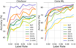
Figure 3. Accuracy on the Semi-supervised Node Classification task by varying the ratio of nodes labeled for training. The embedding dimensionality is $32$.

We further follow prior work (Grover and Leskovec, 2016) in reporting the results when the number of nodes labeled for training is varied between $1\%$ and $10\%$. According to Fig. 3, D-HYPR consistently outperforms the baselines, and tends to perform well at fairly low label rates.

Link Sign Prediction. Table 5 reports the results of SP. D-HYPR is the most effective GNN model. Similar to LP and NC tasks, the effectiveness of D-HYPR is the most striking using a $4$ dimensional embedding space. One interesting observation is that the relative gains of D-HYPR on Wiki NC is much higher than Wiki SP, which suggests that asymmetry preservation can greatly improve the NC results (because unlike the NC task, while learning the asymmetric link sign prediction task, the baselines are able to simultaneously learn asymmetric node connectivity).

Embedding Visualization. In Fig. 1, we visualize $2$D projections of embeddings. Unlike the prior methods (e.g., DGCN, DiGCN, etc.), in whose 2D projected embedding space nodes belonging to different topic classes often severely overlap, D-HYPR leads to the best class separation. This suggests that D-HYPR produces an embedding space that better captures the semantics of the digraph.

Parameter Sensitivity. We first examine how $\lambda$ affects the performance of D-HYPR by varying $\lambda$ from $0.25$ to $10$ (Table 6) while keeping other hyperparameters fixed (32-Dim, the NC task). Larger $\lambda$ place more value on a symmetric embedding distance (which models `homophily' ), whereas a smaller $\lambda$ emphasizes the asymmetric node connectivity (which characterizes `preferential attachment'). The performance of D-HYPR first increases with $\lambda$ and then decreases. Using the $\lambda$ that produces the best result, we then vary $K$. As shown in Table 7, better results are obtained when $K$ is larger, which means a wider receptive field and more scale information. However, an overly large $K$ can lead to feature dilution. It is worth mentioning that D-HYPR still outperforms the SOTA methods by a large margin when $K$=$1$, which suggests the superiority of D-HYPR is not simply coming from the neighbor augmentation that connects nodes to their k-order neighbors. Hyperbolic neighborhood collaboration and preserving asymmetry are important factors that lead to the superiority of D-HYPR.

Ablation Study. As shown in Table 8, removing any neighborhood that we defined harms the performance of D-HYPR. Compared with the approach that learns the proximity matrices (adjacency matrix $A$ $+$ $3$ learnable matrices) or approaches that use other forms of multi-scale proximity matrices (e.g., MagNet, DiGCN and DGCN), D-HYPR performs much better. The proximity matrices are proposed in a way to leverage the inductive biases exhibited in real-world digraphs, thus facilitating the learning process and increasing the accuracy. Replacing hyperbolic with the Euclidean space entails substantial performance drops. Still, this ablation yields better results than GCNs due to the other proposed components (e.g., collaborative learning). Neighborhood collaboration is also crucial. The ablation that removes the hyperbolic neighborhood aggregation component has worse results than our full design, and the ablation that further replaces hyperbolic with the Euclidean space has much lower accuracies. Moreoever, self-supervision helps substantially. D-HYPR is aided by the Gravity regularizer more than the Fermi-Dirac regularizer, as the former captures the asymmetric link connectivity. While the Fermi-Dirac regularizer provides auxiliary benefits, the embedding distance term in the Fermi-Dirac regularizer co-occurs in the Gravity regularizer, which also explains the stronger capability of the latter. All ablations have a lower accuracy than our full model, suggesting that the ablated components work together to increase the learning abilities of D-HYPR.

Discussion. D-HYPR has a statistically superior and more stable performance across datasets and tasks. This is because D-HYPR benefits from the use of hyperbolic space, information collected from the multi-ordered diverse neighborhoods and accounts for directionality. By favoring non-Euclidean over Euclidean geometry for DRL, D-HYPR incurs lower node neighborhoods distortion. In addition, the proposed $4$ canonical types of $k$-order proximity matrix are defined based on the semantics of directed edges in accordance with real-life observations. This allows D-HYPR to leverage inductive biases exhibited in many real-world digraphs, facilitating the learning and increasing the accuracy.

Since D-HYPR addresses Neighborhood Modeling, we provide neighborhood analyses of datasets in Fig. 4, where pie charts show the ratio of the $4$ canonical types of neighborhoods in each dataset ($K$=$1$). Unlike the diffusion in/out neighborhood that traditional GNNs typically use, common in/out neighborhood consists of more neighbors, which suggests that neighborhood collaborative learning benefits from encoding additional context. Nevertheless, a larger neighborhood size does not necessarily entail a greater importance according to the ablation study (Table 8). For each neighborhood type, we also plot a histogram showing the distribution of the number of neighbors a node has over the entire graph. We observe asymptotical power-law node-degree distributions (i.e., scale-free) for most neighborhoods in these digraph datasets.

Table 5. Experimental results on Wiki.

	Model	Node Classification	Link Sign Prediction
4-Dim	GCN (Kipf and Welling, 2016a)	$17.01\pm 0.1$	78.96$\pm$0.4
	GAT (Veličković et al., 2017)	40.75$\pm$10.7	79.38$\pm$0.2
	HGCN (Chami et al., 2019)	36.07$\pm$5.3	$78.72\pm 0.0$
	D-HYPR (ours)	∗71.27$\pm$0.79	∗79.83$\pm$0.0
	Relative Gains ($\%$)	74.90	0.57
8-Dim	GCN (Kipf and Welling, 2016a)	$39.26\pm 9.5$	$78.76\pm 0.1$
	GAT (Veličković et al., 2017)	46.78$\pm$ 10.5	79.41$\pm$0.2
	HGCN (Chami et al., 2019)	58.40$\pm$10.9	79.23$\pm$0.2
	D-HYPR (ours)	∗70.53$\pm$1.6	∗79.47$\pm$0.3
	Relative Gains ($\%$)	20.77	0.08
32-Dim	GCN (Kipf and Welling, 2016a)	$37.77\pm 6.7$	79.39$\pm$ 0.1
	GAT (Veličković et al., 2017)	46.12$\pm$ 8.5	79.66$\pm$ 0.1
	HGCN (Chami et al., 2019)	52.63$\pm$ 5.8	$79.21\pm 0.2$
	D-HYPR (ours)	∗71.65 $\pm$ 1.0	∗79.73 $\pm$ 0.2
	Relative Gains ($\%$)	36.14	0.09

Note: $10$ random dataset splits are used for the SP task. The embedding dimensionality is $32$.

Table 6. Parameter sensitivity analysis in terms of $\lambda$. The superiority of D-HYPR is not sensitive to the hyperparameter $\lambda$.

$\lambda$	0.25	0.50	0.75	1.00	1.25	1.50	1.75	2.00	2.25	2.50	2.75	3.00	3.25	3.50	3.75	4.00	4.25	4.50	4.75	5.00	10.0
CiteSeer	69.74	70.66	70.46	70.44	70.30	70.34	69.99	69.79	69.24	69.61	68.13	68.05	68.12	67.64	67.85	67.67	67.69	67.34	67.18	67.12	66.85
	$\pm$1.6	$\pm$1.2	$\pm$1.3	$\pm$1.4	$\pm$1.1	$\pm$1.3	$\pm$1.4	$\pm$1.6	$\pm$1.6	$\pm$1.2	$\pm$1.4	$\pm$1.3	$\pm$1.9	$\pm$1.8	$\pm$1.8	$\pm$1.9	$\pm$1.9	$\pm$2.3	$\pm$2.1	$\pm$1.7	$\pm$1.5
Cora-ML	81.29	81.18	81.59	81.68	81.83	81.97	82.16	81.65	81.10	81.17	81.59	81.66	81.32	81.93	80.19	80.31	79.13	79.51	80.18	79.78	77.73
	$\pm$1.3	$\pm$1.2	$\pm$1.2	$\pm$1.4	$\pm$1.1	$\pm$1.0	$\pm$1.3	$\pm$1.2	$\pm$1.0	$\pm$1.4	$\pm$1.0	$\pm$1.2	$\pm$ 1.1	$\pm$1.1	$\pm$1.5	$\pm$1.3	$\pm$2.3	$\pm$1.7	$\pm$1.9	$\pm$1.4	$\pm$2.0

Note: the task is Node Classification, and the embedding dimensionality is $32$ (same for Table 7).

Table 7. Parameter sensitivity analysis in terms of $K$. D-HYPR consistently outperforms SOTA methods by a large margin.

$K$	1	2	3
CiteSeer	69.23 $\pm$ 1.5	70.66 $\pm$ 1.2	69.76 $\pm$ 1.5
Cora-ML	82.16 $\pm$ 1.3	82.16 $\pm$ 1.3	82.19 $\pm$ 1.3

Table 8. Ablation study that demonstrates the individual contribution of components in D-HYPR (32-Dim, the NC task).

Method	CiteSeer	Cora-ML
D-HYPR (Our Full Design)	$70.66\pm 1.2$	$82.19\pm 1.3$
No $A_{d_{in}}^{k}$	$68.72\pm 1.2$	$82.11\pm 1.2$
No $A_{d_{out}}^{k}$	$69.10\pm 0.9$	$81.33\pm 1.4$
No $A_{c_{in}}^{k}$	$69.98\pm 1.0$	$81.86\pm 1.6$
No $A_{c_{out}}^{k}$	$69.84\pm 1.3$	$81.74\pm 1.8$
No Hyperbolic Neighborhood Collaboration	$70.13\pm 1.5$	$82.03\pm 1.1$
No Gravity	$68.58\pm 1.3$	$79.21\pm 1.5$
No Fermi-Dirac	$70.03\pm 1.2$	$82.05\pm 1.3$
No Self-Supervision	$67.85\pm 1.9$	$78.15\pm 2.1$
Euclidean	61.86 $\pm$ 5.4	73.38 $\pm$ 6.7
Euclidean and No Neighborhood Collaboration	$51.01\pm 6.2$	$65.46\pm 12.1$
$A$ + Three Learnable Matrices	$60.97\pm 12.7$	$78.92\pm 2.9$

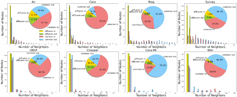
Figure 4. Neighborhood analyses of datasets. The common in/out neighborhood consists of more neighbors than diffusion in/out neighborhood that traditional methods typically use. The $8$ digraph datasets demonstrate a clear scale-free characteristic for most neighborhoods.

Though in principle, MLP can serve as the node-pair score function to learn asymmetric node connectivity (e.g., used by MagNet, DiGCN, etc., in the LP experiments), we resort to Fermi-Dirac and Gravity decoders because the two neatly model the driving forces of link formation, and provide the right level of inductive biases for D-HYPR to more easily generalize well across cases. Fermi-Dirac is particularly suitable for hyperbolic geometry because Fermi-Dirac statistics provide a physical interpretation of hyperbolic distances as energies of links (Krioukov et al., 2009), and the Gravity function is elegantly derived from Newton's theory of universal gravitation with the learnable mass encompassing centrality measures. Overall, D-HYPR leverages the inductive biases exhibited in real-world digraphs and thus generalizes well across tasks; it utilizes multi-ordered partitioned-neighborhoods with hyperbolic neighborhood collaboration to address Neighborhood Modeling, and employs self-supervised learning with sociopsychology-inspired regularizers for Asymmetry Preservation.

7. Conclusion

We propose D-HYPR: the Digraph HYPERbolic Network, as a novel GNN-based formalism for Digraph Representation Learning (DRL) by addressing Neighborhood Modeling and Asymmetry Preservation. Through extensive and rigorous evaluation involving 21 prior techniques, we empirically demonstrate the superiority of D-HYPR. D-HYPR outperforms the current SOTA consistently and statistically significantly on 8 digraph datasets across 4 tasks. In addition, D-HYPR retains effectiveness given a low budget of embedding dimensionality or labeled training samples, which is desirable for real-world applications.

One limitation of D-HYPR is the increased number of parameters, due to the use of multiple neighborhoods. As future work, we would like to explore automatic and dynamic neighborhood partitioning, as well as parameter-sharing mechanisms to improve D-HYPR. Furthermore, theoretical analyses and novel large-scale applications of D-HYPR are avenues worthy of exploration.

Acknowledgment

The research was supported in part by NSF awards: IIS-1703883, IIS-1955404, IIS-1955365, RETTL-2119265, and EAGER-2122119. This material is based upon work supported by the U.S. Department of Homeland Security under Grant Award Number 22STESE00001 01 01.

Disclaimer: The views and conclusions contained in this document are those of the authors and should not be interpreted as necessarily representing the official policies, either expressed or implied, of the U.S. Department of Homeland Security.

References

- (1)
- Bachmann et al. (2020) Gregor Bachmann, Gary Bécigneul, and Octavian Ganea. 2020. Constant curvature graph convolutional networks. In International Conference on Machine Learning. PMLR, 486–496.
- Battaglia et al. (2018) Peter W Battaglia, Jessica B Hamrick, Victor Bapst, Alvaro Sanchez-Gonzalez, Vinicius Zambaldi, Mateusz Malinowski, Andrea Tacchetti, David Raposo, Adam Santoro, Ryan Faulkner, et al. 2018. Relational inductive biases, deep learning, and graph networks. arXiv preprint arXiv:1806.01261 (2018).
- Beani et al. (2021) Dominique Beani, Saro Passaro, Vincent Létourneau, Will Hamilton, Gabriele Corso, and Pietro Liò. 2021. Directional graph networks. In International Conference on Machine Learning. PMLR, 748–758.
- Bronstein et al. (2017) Michael M Bronstein, Joan Bruna, Yann LeCun, Arthur Szlam, and Pierre Vandergheynst. 2017. Geometric deep learning: going beyond euclidean data. IEEE Signal Processing Magazine 34, 4 (2017), 18–42.
- Cai et al. (2018) Hongyun Cai, Vincent W Zheng, and Kevin Chen-Chuan Chang. 2018. A comprehensive survey of graph embedding: Problems, techniques, and applications. IEEE Transactions on Knowledge and Data Engineering 30, 9 (2018), 1616–1637.
- Chamberlain et al. (2017) Benjamin Paul Chamberlain, James Clough, and Marc Peter Deisenroth. 2017. Neural embeddings of graphs in hyperbolic space. arXiv preprint arXiv:1705.10359 (2017).
- Chami et al. (2020) Ines Chami, Adva Wolf, Da-Cheng Juan, Frederic Sala, Sujith Ravi, and Christopher Ré. 2020. Low-Dimensional Hyperbolic Knowledge Graph Embeddings. In Proceedings of the 58th Annual Meeting of the Association for Computational Linguistics. 6901–6914.
- Chami et al. (2019) Ines Chami, Zhitao Ying, Christopher Ré, and Jure Leskovec. 2019. Hyperbolic graph convolutional neural networks. In Advances in neural information processing systems. 4868–4879.
- Chen et al. (2021) Weize Chen, Xu Han, Yankai Lin, Hexu Zhao, Zhiyuan Liu, Peng Li, Maosong Sun, and Jie Zhou. 2021. Fully Hyperbolic Neural Networks. arXiv preprint arXiv:2105.14686 (2021).
- Dai et al. (2021) Jindou Dai, Yuwei Wu, Zhi Gao, and Yunde Jia. 2021. A Hyperbolic-to-Hyperbolic Graph Convolutional Network. In Proceedings of the IEEE/CVF Conference on Computer Vision and Pattern Recognition. 154–163.
- Defferrard et al. (2016) Michaël Defferrard, Xavier Bresson, and Pierre Vandergheynst. 2016. Convolutional neural networks on graphs with fast localized spectral filtering. Advances in neural information processing systems 29 (2016), 3844–3852.
- Ganea et al. (2018a) Octavian Ganea, Gary Bécigneul, and Thomas Hofmann. 2018a. Hyperbolic entailment cones for learning hierarchical embeddings. In International Conference on Machine Learning. PMLR, 1646–1655.
- Ganea et al. (2018b) Octavian Ganea, Gary Bécigneul, and Thomas Hofmann. 2018b. Hyperbolic neural networks. In Advances in neural information processing systems. 5345–5355.
- Gong and Cheng (2019) Liyu Gong and Qiang Cheng. 2019. Exploiting edge features for graph neural networks. In Proceedings of the IEEE/CVF Conference on Computer Vision and Pattern Recognition. 9211–9219.
- Grover and Leskovec (2016) Aditya Grover and Jure Leskovec. 2016. node2vec: Scalable feature learning for networks. In Proceedings of the 22nd ACM SIGKDD international conference on Knowledge discovery and data mining. 855–864.
- Gu et al. (2018) Albert Gu, Frederic Sala, Beliz Gunel, and Christopher Ré. 2018. Learning mixed-curvature representations in product spaces. In International Conference on Learning Representations.
- Hamilton et al. (2017) Will Hamilton, Zhitao Ying, and Jure Leskovec. 2017. Inductive representation learning on large graphs. In Advances in neural information processing systems. 1024–1034.
- Jiang et al. (2016) Rui Jiang, Weijie Fu, Li Wen, Shijie Hao, and Richang Hong. 2016. Dimensionality reduction on anchorgraph with an efficient locality preserving projection. Neurocomputing 187 (2016), 109–118.
- Khosla et al. (2019) Megha Khosla, Jurek Leonhardt, Wolfgang Nejdl, and Avishek Anand. 2019. Node representation learning for directed graphs. In Joint European Conference on Machine Learning and Knowledge Discovery in Databases. Springer, 395–411.
- Kim et al. (2018) Junghwan Kim, Haekyu Park, Ji-Eun Lee, and U Kang. 2018. Side: representation learning in signed directed networks. In Proceedings of the 2018 World Wide Web Conference. 509–518.
- Kingma and Ba (2014) Diederik P Kingma and Jimmy Ba. 2014. Adam: A method for stochastic optimization. arXiv preprint arXiv:1412.6980 (2014).
- Kipf and Welling (2016a) Thomas N Kipf and Max Welling. 2016a. Semi-supervised classification with graph convolutional networks. arXiv preprint arXiv:1609.02907 (2016).
- Kipf and Welling (2016b) Thomas N Kipf and Max Welling. 2016b. Variational graph auto-encoders. arXiv preprint arXiv:1611.07308 (2016).
- Klicpera et al. (2018) Johannes Klicpera, Aleksandar Bojchevski, and Stephan Günnemann. 2018. Predict then propagate: Graph neural networks meet personalized pagerank. arXiv preprint arXiv:1810.05997 (2018).
- Kriege et al. (2020) Nils M Kriege, Fredrik D Johansson, and Christopher Morris. 2020. A survey on graph kernels. Applied Network Science 5, 1 (2020), 1–42.
- Krioukov et al. (2010) Dmitri Krioukov, Fragkiskos Papadopoulos, Maksim Kitsak, Amin Vahdat, and Marián Boguná. 2010. Hyperbolic geometry of complex networks. Physical Review E 82, 3 (2010), 036106.
- Krioukov et al. (2009) Dmitri Krioukov, Fragkiskos Papadopoulos, Amin Vahdat, and Marián Boguná. 2009. Curvature and temperature of complex networks. Physical Review E 80, 3 (2009), 035101.
- Law and Stam (2020) Marc T Law and Jos Stam. 2020. Ultrahyperbolic Representation Learning. Advances in neural information processing systems (NeurIPS 2020) (2020).
- Liu et al. (2019) Qi Liu, Maximilian Nickel, and Douwe Kiela. 2019. Hyperbolic graph neural networks. arXiv preprint arXiv:1910.12892 (2019).
- Ma et al. (2019a) Jianxin Ma, Peng Cui, Kun Kuang, Xin Wang, and Wenwu Zhu. 2019a. Disentangled graph convolutional networks. In International Conference on Machine Learning. PMLR, 4212–4221.
- Ma et al. (2019b) Yi Ma, Jianye Hao, Yaodong Yang, Han Li, Junqi Jin, and Guangyong Chen. 2019b. Spectral-based graph convolutional network for directed graphs. arXiv preprint arXiv:1907.08990 (2019).
- McPherson et al. (2001) Miller McPherson, Lynn Smith-Lovin, and James M Cook. 2001. Birds of a feather: Homophily in social networks. Annual review of sociology 27, 1 (2001), 415–444.
- Mitzenmacher (2004) Michael Mitzenmacher. 2004. A brief history of generative models for power law and lognormal distributions. Internet mathematics 1, 2 (2004), 226–251.
- Nickel and Kiela (2017) Maximillian Nickel and Douwe Kiela. 2017. Poincaré embeddings for learning hierarchical representations. In Advances in neural information processing systems (NeurIPS 2017). 6338–6347.
- Nickel and Kiela (2018) Maximillian Nickel and Douwe Kiela. 2018. Learning continuous hierarchies in the lorentz model of hyperbolic geometry. In International Conference on Machine Learning. PMLR, 3779–3788.
- Ou et al. (2016) Mingdong Ou, Peng Cui, Jian Pei, Ziwei Zhang, and Wenwu Zhu. 2016. Asymmetric transitivity preserving graph embedding. In Proceedings of the 22nd ACM SIGKDD international conference on Knowledge discovery and data mining. 1105–1114.
- Perozzi et al. (2014) Bryan Perozzi, Rami Al-Rfou, and Steven Skiena. 2014. Deepwalk: Online learning of social representations. In Proceedings of the 20th ACM SIGKDD international conference on Knowledge discovery and data mining. 701–710.
- Rossi et al. (2020) Emanuele Rossi, Fabrizio Frasca, Ben Chamberlain, Davide Eynard, Michael Bronstein, and Federico Monti. 2020. SIGN: Scalable Inception Graph Neural Networks. arXiv preprint arXiv:2004.11198 (2020).
- Sala et al. (2018) Frederic Sala, Chris De Sa, Albert Gu, and Christopher Ré. 2018. Representation tradeoffs for hyperbolic embeddings. In International conference on machine learning. PMLR, 4460–4469.
- Salha et al. (2019) Guillaume Salha, Stratis Limnios, Romain Hennequin, Viet-Anh Tran, and Michalis Vazirgiannis. 2019. Gravity-inspired graph autoencoders for directed link prediction. In Proceedings of the 28th ACM International Conference on Information and Knowledge Management. 589–598.
- Shervashidze et al. (2011) Nino Shervashidze, Pascal Schweitzer, Erik Jan Van Leeuwen, Kurt Mehlhorn, and Karsten M Borgwardt. 2011. Weisfeiler-lehman graph kernels. Journal of Machine Learning Research 12, 9 (2011).
- Shi et al. (2019) Lei Shi, Yifan Zhang, Jian Cheng, and Hanqing Lu. 2019. Skeleton-based action recognition with directed graph neural networks. In Proceedings of the IEEE/CVF Conference on Computer Vision and Pattern Recognition. 7912–7921.
- Sim et al. (2021) Aaron Sim, Maciej L Wiatrak, Angus Brayne, Páidí Creed, and Saee Paliwal. 2021. Directed graph embeddings in pseudo-riemannian manifolds. In International Conference on Machine Learning. PMLR, 9681–9690.
- Sun et al. (2019) Jiankai Sun, Bortik Bandyopadhyay, Armin Bashizade, Jiongqian Liang, P Sadayappan, and Srinivasan Parthasarathy. 2019. Atp: Directed graph embedding with asymmetric transitivity preservation. In Proceedings of the AAAI Conference on Artificial Intelligence, Vol. 33. 265–272.
- Suzuki et al. (2019) Ryota Suzuki, Ryusuke Takahama, and Shun Onoda. 2019. Hyperbolic disk embeddings for directed acyclic graphs. In International Conference on Machine Learning. PMLR, 6066–6075.
- Thost and Chen (2021) Veronika Thost and Jie Chen. 2021. Directed Acyclic Graph Neural Networks. International Conference on Learning Representations (2021).
- Tong et al. (2021) Zekun Tong, Yuxuan Liang, Henghui Ding, Yongxing Dai, Xinke Li, and Changhu Wang. 2021. Directed Graph Contrastive Learning. Advances in Neural Information Processing Systems (NeurIPS) 34 (2021).
- Tong et al. (2020a) Zekun Tong, Yuxuan Liang, Changsheng Sun, Xinke Li, David Rosenblum, and Andrew Lim. 2020a. Digraph Inception Convolutional Networks. Advances in Neural Information Processing Systems 33 (2020).
- Tong et al. (2020b) Zekun Tong, Yuxuan Liang, Changsheng Sun, David S Rosenblum, and Andrew Lim. 2020b. Directed Graph Convolutional Network. arXiv preprint arXiv:2004.13970 (2020).
- Vaswani et al. (2017) Ashish Vaswani, Noam Shazeer, Niki Parmar, Jakob Uszkoreit, Llion Jones, Aidan N Gomez, Łukasz Kaiser, and Illia Polosukhin. 2017. Attention is all you need. In Advances in neural information processing systems. 5998–6008.
- Veličković et al. (2017) Petar Veličković, Guillem Cucurull, Arantxa Casanova, Adriana Romero, Pietro Lio, and Yoshua Bengio. 2017. Graph attention networks. arXiv preprint arXiv:1710.10903 (2017).
- Veličković et al. (2018) Petar Veličković, William Fedus, William L Hamilton, Pietro Liò, Yoshua Bengio, and R Devon Hjelm. 2018. Deep graph infomax. arXiv preprint arXiv:1809.10341 (2018).
- Wold et al. (1987) Svante Wold, Kim Esbensen, and Paul Geladi. 1987. Principal component analysis. Chemometrics and intelligent laboratory systems 2, 1-3 (1987), 37–52.
- Wu et al. (2019) Felix Wu, Tianyi Zhang, Amauri Holanda de Souza Jr, Christopher Fifty, Tao Yu, and Kilian Q Weinberger. 2019. Simplifying graph convolutional networks. arXiv preprint arXiv:1902.07153 (2019).
- Wu et al. (2020) Zonghan Wu, Shirui Pan, Fengwen Chen, Guodong Long, Chengqi Zhang, and S Yu Philip. 2020. A comprehensive survey on graph neural networks. IEEE Transactions on Neural Networks and Learning Systems (2020).
- Yang et al. (2017) Cheng Yang, Maosong Sun, Zhiyuan Liu, and Cunchao Tu. 2017. Fast network embedding enhancement via high order proximity approximation.. In IJCAI. 3894–3900.
- Ying et al. (2021) Chengxuan Ying, Tianle Cai, Shengjie Luo, Shuxin Zheng, Guolin Ke, Di He, Yanming Shen, and Tie-Yan Liu. 2021. Do Transformers Really Perform Bad for Graph Representation? (2021).
- Zhang et al. (2021a) Xitong Zhang, Nathan Brugnone, Michael Perlmutter, and Matthew Hirn. 2021a. MagNet: A Magnetic Neural Network for Directed Graphs. Advances in Neural Information Processing Systems 34 (2021).
- Zhang et al. (2021b) Yiding Zhang, Xiao Wang, Chuan Shi, Xunqiang Jiang, and Yanfang Fanny Ye. 2021b. Hyperbolic graph attention network. IEEE Transactions on Big Data (2021).
- Zhang et al. (2021c) Yiding Zhang, Xiao Wang, Chuan Shi, Nian Liu, and Guojie Song. 2021c. Lorentzian Graph Convolutional Networks. In Proceedings of the Web Conference 2021. 1249–1261.
- Zhou et al. (2017) Chang Zhou, Yuqiong Liu, Xiaofei Liu, Zhongyi Liu, and Jun Gao. 2017. Scalable graph embedding for asymmetric proximity. In Proceedings of the AAAI Conference on Artificial Intelligence, Vol. 31.
- Zhou et al. (2020) Jie Zhou, Ganqu Cui, Shengding Hu, Zhengyan Zhang, Cheng Yang, Zhiyuan Liu, Lifeng Wang, Changcheng Li, and Maosong Sun. 2020. Graph neural networks: A review of methods and applications. AI Open 1 (2020), 57–81.
- Zhu et al. (2020) Shichao Zhu, Shirui Pan, Chuan Zhou, Jia Wu, Yanan Cao, and Bin Wang. 2020. Graph Geometry Interaction Learning. In Advances in Neural Information Processing Systems.