Stochastic modelling of spreading and dissipation
in mixed-chaotic system that are driven quasi-statically

Abstract

We analyze energy spreading for a system that features mixed chaotic phase-space, whose control parameters (or slow degrees of freedom) vary quasi-statically. For demonstration purpose we consider the restricted 3 body problem, where the distance between the two central stars is modulated due to their Kepler motion. If the system featured hard-chaos, one would expect diffusive spreading with coefficient that can be estimated using linear-response (Kubo) theory. But for mixed phase space the chaotic sea is multi-layered. Consequently, it becomes a challenge to find a robust procedure that translates the sticky dynamics into a stochastic model. We propose a Poincaré-sequencing method that reduces the multi-dimensional motion into a one-dimensional random-walk in impact-space. We test the implied relation between stickiness and the rate of spreading.

I Introduction

Considering a closed Hamiltonian driven system, such as a particle in a box with moving wall (the piston paradigm), the textbook assumption is that quasi-static processes are adiabatic, and therefore reversible. This claim can be established for an integrable system by recognizing that the action-variables are adiabatic invariants [1]. At the opposite extreme, analysis of slowly driven completely chaotic systems [2, 3, 4] has led to a mesoscopic version of Kubo linear-response theory and its associated fluctuation-dissipation phenomenology [5, 6, 7, 8]. However, generic systems are neither integrable nor completely chaotic. Rather their phase space is mixed, resulting in the failure of the adiabatic picture [9, 10, 11, 12, 13], and of linear-response theory. Namely, the phase space structure varies with the control parameter: tori are destroyed; chaotic corridors are opened allowing migration between different regions in phase space [14, 15]; stochastic regions merge into chaos; sticky regions are formed [16, 17, 18, 19, 20]; sets of tori re-appear or emerge. Some of those issues can be regarded as a higher-dimensional version of non-linear scenarios that are relate to bifurcations of fixed points, notably swallow-tail loops [21, 22, 23, 24, 25], or as a higher-dimensional version of the well-studied separatrix crossing [26, 27, 28, 29, 30, 31, 32, 33, 34, 35, 36, 37], where the Kruskal-Neishtadt-Henrard theorem is followed.

Motivation.– The analysis of driven systems that feature an underlying mixed-chaotic phase-space is a rather universal theme, that has relevance to many fields in physics. There are mainly two ways to motivate the quasi-static perspective for the pertinent degrees of freedom (dof). For some systems it is natural to distinguish between slow (‘heavy’) dof, and fast (‘light’) dof. Then it makes sense to regard the heavy dof as parametric driving, and to ignore the back reaction. The heavy dof might be the location of a piston, or it might be the distance between the two stars that perform Kepler motion in the restricted 3 body problem (which we discuss below).

A different way to motivate this perspective originates from mesoscopic physics. One would like to provide a comprehensive set of tools for the design and for the optimization of quasi-static protocols, e.g. in the context of Bose-Hubbard systems [38, 39, 40]. The feasibility and the efficiency of such protocols is related to the underlying mixed-chaotic phase-space dynamics, as demonstrated in [12, 15, 13].

Model systems.– The simplest way to demonstrates anomalies that may arise in the quasi-static limit is to study billiard systems [9, 11]. The geometric construction allows a sharp distinction between regions in (phase)space. For example, the Bunimovich mushroom geometry of [11] is composed of a regular region (the mushroom cap), and a chaotic region (stadium-like stem). However, such model is in some sense not generic. More generally, phase space has hierarchical structure with peripheral sticky regions [16] (and see Refs.[1-10] therein); and the composition of the energy surface depends on energy. Furthermore, in practice the distinction between the “sea” and the “islands” is not sharp neither fully controlled. This requires the development of new tools, to facilitate the analysis of the time-dependent dynamics.

For the purpose of developing tools for the analysis of quasi-static scenarios, Billiards are too simple, while Bose-Hubbard systems are over-complicated and too demanding. A mathematically-oriented strategy would be to select an artificial Hamiltonian. But it is much more appealing to consider a toy Hamiltonian that has physical significance. At this point, it is appropriate to recall that the discussion of Hamiltonian chaos is historically rooted in the 3 body problem of celestial mechanics.

The restricted 3 body problem.– It is natural to select Hill’s Hamiltonian [41, 42, 43] as a prototype model for analysis. This Hamiltonian describes the motion of a test-particle in the field of force of a binary systems (stars that perform Kepler motion). In reality the test particle might be a satellite or a circumbinary planet [44, 45, 46]. Optionally, in order to emphasize the analogy with the piston paradigm, we can have in mind a binary system immersed in a cloud of dust: the dust is driven quasi-statically by the Kepler motion of the stars. In reality the ‘dust’ might be an asteroid system, and the binary system might consist of massive black holes at the center of a galactic nuclei.

Hill’s Hamiltonian, unlike the Bose-Hubbard Hamiltonian, is simple for visualization, and still possesses all the generic features of realistic models. The test-particle might perform quasi-regular motion around one of the stars, or chaotic motion wandering between the two stars. We find, as expected, a textured phase space structure with sticky peripheral regions. As an additional bonus this model also allows to consider a disintegration scenario: the test particles gains energy and eventually escapes to infinity.

The full 3 body problem.– The analysis of the Hill’s Hamiltonian has possibly importance in the restricted sense, but we would like to suggest that its quasi-static perspective might be of interest also for the full 3 body problem. Here we would like to refer to the recent works of [47, 48] (and see references therein). Given the total energy and the total angular momentum, the challenge is to calculate, say, the probability $\sigma(E)$ that one of the stars is ejected with an energy $E$. For this purpose it has been assumed that phase space is composed of a totally chaotic interaction region, and an outer region where one of the bodies becomes an outsider (possibly unbounded). Assuming that the motion in the interaction region completely ergodizes the energy, the probability $\sigma(E)$, up to normalization, is given by the corresponding phase-space volume, that can be calculated analytically.

Let us speculate that in some cases the dynamics of the escaping body, while in the interaction region, is described by the Hill’s Hamiltonian. Then the question arises, how its energy $E$ is affected by the motion of the binary system. It is possibly more transparent to re-phrase this questions using the language of statistical mechanics. Namely, considering a cloud of trajectories, we would like to analyse the spreading in energy.

Clearly the assumption of total randomization of $E$ is an over-simplification for several reasons. First of all, integrable islands should be excluded. But even if we ignore the islands, we are going to show that the spreading dynamics is not trivial. Roughly speaking we are going to characterize the energy distribution by its “width”, and by its “average”. One expects a fluctuation-dissipation relation that related the rate of energy increase to the rate of the spreading [5, 6, 7, 8]. But this relation is endangered by the mixed phase space dynamics.

Outline.– In Sec. (II) we introduce the generalized Hill’s Hamiltonian. This Hamiltonian will be used as a test case for the application of our approach. It features a mixed chaotic phase space whose parametric evolution can be visualized using a Poincaré landscape plot. In Sec. (III) we use a Poincaré-sequencing method in order to encode the time dependent dynamics. Consequently, the multi-dimensional motion in phase space is reduced into a one-dimensional random-walk in impact-space. This inspires the introduction of an effective stochastic model in Sec. (IV) and Sec. (V), which is used in Sec. (VI) to provide an explicit relation between stickiness and the rate of spreading. In Sec. (VII) we explain that the dependence on the directionality of a cycle is linked to asymmetry that can be detected in the Poincaré-sequencing analysis. For completeness we present in Sec. (VIII) the theoretical reasoning that relates the rate of dissipation to the stochastic characterisation of the dynamics.

II The generalized Hill problem

The Hamiltonian under consideration concerns the motion of a test particle (satellite) in the vicinity of massive bodies (stars). The stars are performing a cycle $(X(t),Y(t))$ that has frequency $\Omega$ and constant angular momentum $\ell$. It might be, but not have to be, the Kepler motion of Appendix A. We define the characteristic radius $c$ such that the scaled angular momentum is ${\ell\equiv c^{2}\Omega}$. In polar coordinates the cycle is parameterized by ${R(t)=c\mathsf{R}(\theta(t))}$. By definition of $c$, one observes that the $d\theta/(2\pi)$ integral over $|\mathsf{R}(\theta)|^{2}$ is unity. Regarding $\theta$ as the time variable, one obtains, after a sequence of transformations (see Appendix B), the generalized Hill’s Hamiltonian:

$$\mathcal{H}=\frac{1}{2}(\bm{p}-\bm{r}_{\perp})^{2}+g\mathsf{R}(\theta)u(\bm{r})-\frac{1}{2}\mathsf{K}(\theta)\bm{r}^{2}\ \ \ \ \$$ (1)

where (prime indicates theta derivative):

$$\mathsf{K}(\theta)\ =\ 1+\left(\frac{1}{\mathsf{R}(\theta)}\right)^{\prime\prime}\mathsf{R}(\theta)$$ (2)

and the scaled version of the attractive potential is

$$u(\bm{r})=-\frac{\mu_{2}}{\sqrt{(x-\mu_{1})^{2}+y^{2}}}-\frac{\mu_{1}}{\sqrt{(x+\mu_{2})^{2}+y^{2}}}\ \ \ \$$ (3)

with ${\mu_{1}+\mu_{2}=1}$. The parameter $g$ is the scaled attraction constant for the force between the satellite and the stars. It can be due to gravitation, or (in different context) it can be of Coulomb origin.

For an arbitrary quasi-Kepler motion (as defined above, meaning that $\ell$ is constant) the Hamiltonian is controlled by two parameters $(\mathsf{R},\mathsf{K})$. So in general the satellite experiences a cycle. But for a proper Kepler motion ${\mathsf{K}(\theta)=g_{\varepsilon}\mathsf{R}(\theta)=1/[1+\varepsilon\cos(\theta)]}$ with ${g_{\varepsilon}=(1-\varepsilon^{2})^{-3/4}}$. Consequently, see Appendix C, we get a Hamiltonian that depends on a single parameter,

$$\mathcal{H}(\bm{r},\bm{p})=\frac{1}{2}(\bm{p}-\bm{r}_{\perp})^{2}+\mathsf{R}(\theta)\left(gu(\bm{r})-\frac{1}{2}g_{\varepsilon}\bm{r}^{2}\right)\ \ \ \$$ (4)

Thus, a proper Kepler motion should be regarded as a modulation and not as a cycle.

In the last paragraph of Appendix C we explain that the dimensionless slowness parameter that indicates a quasi-static Kepler driving is ${\varepsilon g_{\varepsilon}/g}$. For simulations we used $g{=}25$, and $\varepsilon{=}0.2$, and $\mu_{1}{=}\mu_{2}{=}1/2$.

Figure 1: Poincaré landscape. The upper panel is a standard Poincaré section for Hill’s Hamiltonian Eq. ​​(1) with ${\mu_{1}{=}\mu_{2}{=}1/2}$, and $\varepsilon{=}0.2$, and $g{=}25$, at energy $E{=}-22.2$. The control parameter $\mathsf{R}$ is frozen at the value ${\theta=0}$. In the middle panel each row is a $p_{x}{=}0$ stripe of the Poincaré section at different $E$, while $\mathsf{R}$ is frozen at the value $\theta{=}0$. In the lower panel the Poincaré stripes are plotted for frozen $\mathsf{R}$ at different values of $\theta$. Initially $E{=}-22.2$, and later we follow $E$ adiabatically. The color code is such that chaotic trajectories are red, while quasi-regular chaotic trajectories are blue.

Poincaré landscape.– Fig. ​​1 displays a representative Poincaré section for the time-independent ($\theta$-frozen) Hill’s Hamiltonian. The phase space structure is as follows: two (blue) regions contain quasi-regular trajectories around each of the two stars; there are additional quasi-regular regions; and there is a large (red) chaotic sea. In order to demonstrate the variation of phase space with respect to the energy $E$, or with respect to a control parameter (here it is $\theta$ that parameterize the Kepler motion), we propose to look on the Poincaré landscape that is displayed in the additional panels of Fig. ​​1. Each row in those additional panels encodes the information regarding the phase-space structure for a different value of $E$ or $\theta$, respectively.

In a later section we display on top of this landscape, an evolving cloud that is propagated by the time-depended Hamiltonian $\mathcal{H}(\bm{r},\bm{p};\theta(t))$, with $\dot{\theta}{=}1$ as implied by our definitions of scaled time. In this time dependent scenario, points of the cloud can spread in energy, and migrate between different regions.

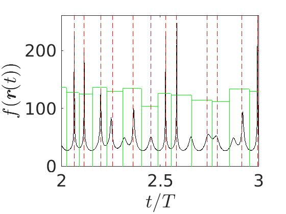
Figure 2: Poincaré pulses. Representative piece of the signal ${f(\bm{r}(t))}$. The vertical red lines indicate the moments $t_{j}$ that are selected by the Poincaré section. The signal is regarded as a sequence of rectangular pulses (green line). Each pulse has duration $T_{j}$ and average height ${\bar{F}_{j}=F_{j}/T_{j}}$. In the figure $\bar{F}$ is scaled vertically ($\times 3$) to improve resolution.

III Poincaré sequencing

The spreading of energy of a driven system is determined by the fluctuations of the generalized force $\mathcal{F}$ that is associated with the control variable $\theta$. Note that we assume periodic driving, and that the scaled Hamiltonian is defined such that $\dot{\theta}{=}1$. For typical model systems, e.g. Billiards with moving piston, and also for the Hill’s Hamiltonian, we can factorize $\mathcal{F}$ as follows:

$$\mathcal{F}\ \ =\ \ -\frac{\partial\mathcal{H}}{\partial\theta}\ \ \equiv\ \ h(\theta)f(\bm{r})$$ (5)

where ${f(r)=(g/g_{\varepsilon})u(r)-(1/2)r^{2}}$. The variation of the energy is an integral over $-\dot{\theta}\mathcal{F}(t)$, but for the analysis it is more convenient to consider

$$Q\ \ =\ \ \int_{0}^{t}f(\bm{r}(t))dt\ \ \equiv\ \ \sum_{j}F_{j}$$ (6)

The last equality expresses the integral as a sum over pulses, whose area is defined in the illustration of Fig. ​​2.

The variation of $Q$, unlike that of $E$ does not include $\dot{\theta}$ as a prefactor, and therefore allows, on equal footing, to compare the fluctuations of the driven system to the fluctuations that are generated by the time independent (frozen $\theta$) Hamiltonian.

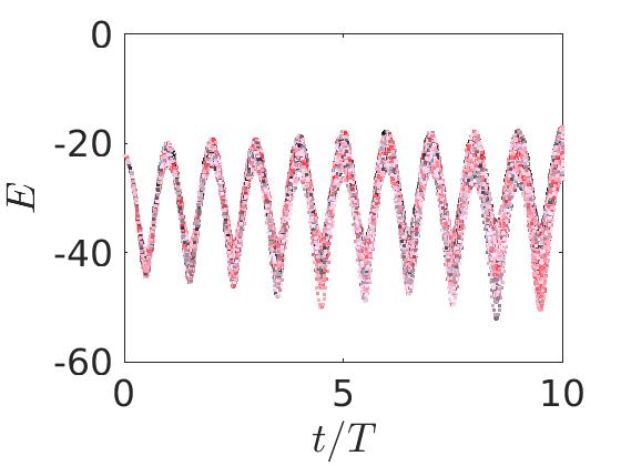
Figure 3: Variation of the energy. The energy for a cloud of chaotic trajectories is plotted as a function of time (upper panel). The spreading is displayed in the lower panel (black line). Here we define $S_{E}$ as the width of the central region that supports 50% of the distribution. The blue line is a moving average.

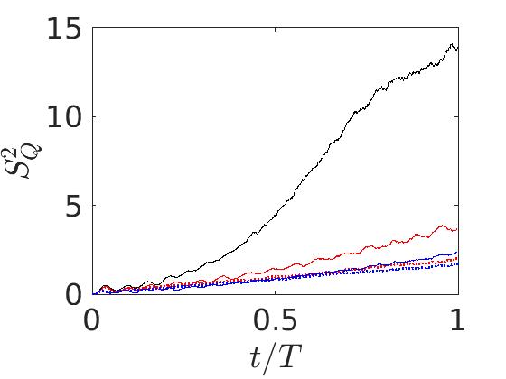
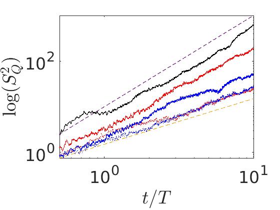
Figure 4: Spreading. The dynamics is generated by Eq. ​​(1), with the same parameters as in Fig. ​​1. The time dependence of $S_{Q}$ is regarded as a measure for spreading, where $Q$ is defined by Eq. ​​(6). The black line is $S_{Q}$ for an ensemble of 1-cycle (normal panel) and 10-cycles (log-log panel) trajectories that were launched in the chaotic sea. In the log-scale panel, the lower and upper dashed lines indicate $\propto t$ and $\propto t^{2}$ dependence. The red and blue lines are $S_{Q}$ if the control parameter $\mathsf{R}$ were frozen. The selected values are at $\theta{=}0$ (red) and $\theta{=}\pi$ (blue), for which the spreading is relatively fast/slow respectively. According to the traditional paradigm of quasi-static processes, the black line should be roughly between the red and the blue lines, which is clearly not the case. The red and blue dotted lines (lower data lines in both panels) are $S_{Q}$ for a signal that is composed of a randomized sequence of the same pulses, i.e. they provide the variance that would be expected if the actual signal did not have phase-space correlations. We conclude that correlations are enhanced due to the time dependence of $\theta(t)$.

Simulations.– In the simulations we consider the following scenario. Initially we launch a narrow cloud in the middle of the chaotic sea. After a short transient, keeping $\theta$ frozen, this cloud fills most of the chaotic sea. Some extra time might be required in order to penetrate into peripheral regions where the dynamics is sticky. We shall come back to this stickiness issue later on. Subsequently, we run the simulation with the time-dependent Hamiltonian ($\theta$ unfrozen). Due to the driving, the cloud further evolves as follows: (a) Spreading away from the initial energy surface; (b) Migration between separated phase space regions. The dissipation aspect (growth of the average-energy) is directly related to #a and indirectly related to #b.

The spreading measure $S_{Q}$.– The traditional measure for phase space spreading is entropy, but we prefer to adopt a measure that has a direct practical meaning. The natural choice is to look on the energy. We define $S_{E}$ as the width of the energy distribution, namely, it is the range around the median where $50\%$ of the distribution is located (third quartile minus first quartile). In Fig. ​​3 we display $E$ for the trajectories of the cloud, and extract the spreading $S_{E}$ as a function of time. Both feature intra-cycle modulation that is mainly related to the $h(\theta)$ of Eq. ​​(5). In order to get rid of this modulation we prefer to look on $Q$. In Fig. ​​4 we display $S_{Q}$ as a function of time. It is defined as the width that holds $50\%$ of the distribution. Its variation in time, unlike that of $S_{E}$ is rather smooth, and better reflects the systematic spreading of the distribution over phase-space cells. Another advantage is that we can compare the $S_{Q}$ of the driven system with the $S_{Q}$ of the forozen-$\theta$ Hamiltonian. Clearly in the latter context $S_{Q}$ is not a measure for spreading, but a measure for the fluctuations of $\mathcal{F}$.

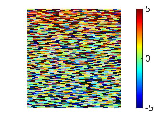
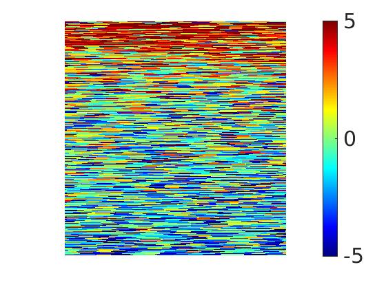
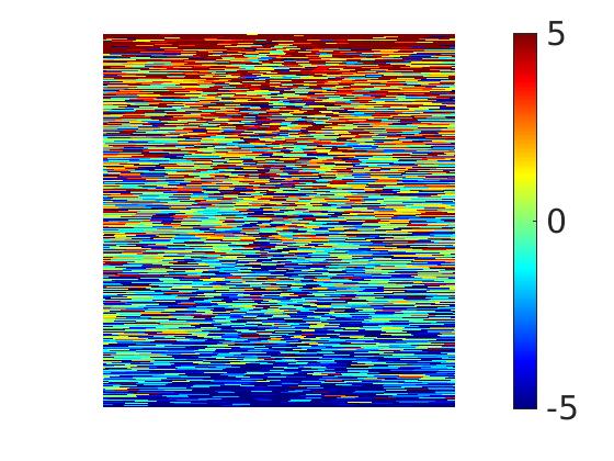
Figure 5: Poincaré sequences of pulses. The rows of each image displays the color-coded sequences $\bar{F}_{j}$ of the length-$T$ trajectories for which the spreading has been calculated in the upper panel of Fig. ​​4. The 3 panels are for $\theta{=}\pi$, and for $\theta{=}0$, and for the actual $\theta(t)$ of the Kepler motion. The trajectories in each panel are ordered by the average value of $\bar{F}_{j}$. The red stretches for $\theta{=}0$ indicate stickiness in red regions that will be identified in Fig. ​​6. The additional blue stretches in the lower panel indicate excess dwell time in the chaotic sea.

Optional perspective on $S_{Q}$.– A very long chaotic trajectory that explores the whole chaotic sea can be regarded as a Poincaré sequence of $F_{j}$ pulses that is characterized by the $S_{Q}(t)$ of Fig. ​​4. In order to get $S_{Q}(t)$, the chaotic trajectory can be divided into sub-sequences of length $T$ (upper panel) or of length $10T$ (lower panel), where $T$ is the period of a cycle. Equivalently, as described in the previous paragrpah, we start the simulation with a cloud of initial points at the middle of the chaotic sea, evolve them, and care to exclude the initial transient.

Detecting correlations.– In order to figure out whether temporal correlations are important we randomize the original $F_{j}$ sequence, and then divide it again into sub-sequences. In Fig. ​​4, the spreading of the randomized-trajectories is displayed too, for sake of comparison. The ratio between the actual rate of spreading, and that of the randomized-trajectories, is a robust measure for correlations.

We would like to “see” the correlation by looking on the “signal”. For this purpose we plot images of the non-randomized sub-sequences in Fig. ​​5. The sub-sequences are ordered according to their average. If the sub-sequences originated from a randomized-trajectory, this average would be close to zero, and the ordering would not result in any visual effect. But sequences of the non-randomized-trajectory are correlated. The correlations can be identified by inspection of the figure. Specifically, the sequences of the time-independent $\theta{=}0$ Hamiltonian exhibit long red stretches, and the Kepler-driven sequences exhibit also blue stretches. This should be contrasted with the sequences of the $\theta{=}\pi$ Hamiltonian, that look rather uncorrelated.

Figure 6: Poincaré mapping of pulses. The upper panel displays the Poincaré section for the ${\theta=0}$ Hamiltonian. Those are the same chaotic trajectories as in Fig. ​​1 (the quasi-integrable regions are left empty), but the points are color-coded by the values of $\bar{F}_{j}$. The black line indicates the border of the energy surface (the forbidden region is outside). The lower panel shows a chaotic trajectory $(x(t),y(t))$. The color encodes the time. The black stretch indicates motion in the “red” sticky region of the upper panel. It is characterized by an ”$\infty$” shaped loops.

Figure 7: Driven system dynamics. In the upper panel a trajectory of the Kepler-driven Hamiltonian is presented using the same section as that of Fig. ​​6. Gray color is used for all the points of the trajectory, while red and blue colors are used for the correlated stretches of Fig. ​​5. Parameters are the same as in Fig. ​​1. The Hamiltonian is time dependent. Accordingly, the cloud of trajectories spreads in energy, and can migrate between different regions. This is demonstrated in the lower panel, where we use the same presentation method as in Fig. ​​1. The native chaotic region, that corresponds to the red areas in Fig. ​​1, is colored in black. The evolving cloud of the Kepler-driven system is displayed using blue, red and gray dots. Red color indicates sticking in periphery regions, while blue indicates sticking in the native chaotic sea. The non-sticking gray points expand into “swamp” regions that are located outside of the native chaotic sea. See text for further details.

Phase space exploration.– Having identified correlations in the ‘signal’, we would like to trace their phase space origin. For this purpose we point out that the value $F$ of the pulse provides information about the location of the phase space region that supports the pulse, as demonstrated in Fig. ​​6. Roughly speaking, we can regard $F$ as a radial coordinate for points in the Poincaré section. Variations in the value of $F$ indicate migration of the trajectory between different regions. In this specific example, red pulses originate from peripheral regions of the chaotic sea, while blue pulses originate from the central region of the chaotic sea. Thus, the red and blue stretches in Fig. ​​5 indicate stickiness in phase-space regions that have distinct typical non-zero value of $F$.

The stickiness to peripheral regions is expected. It has been studied in past literature. What we find rather surprising is the extra stickiness that we find in the dynamics that is generated by the Kepler driven system: the additional blue stretches indicate excess dwell time in the central region of the chaotic sea.

A more careful inspection, see Fig. ​​7, reveals that the stickiness in the central region of the chaotic sea is in the region that was chaotic also in the absence of driving. So roughly we have the following regions: (a) Native chaotic sea region; (b) Swamp chaotic region; (c) Peripheral chaotic regions; (d) Quasi regular regions. The swamp regions appear due to the driving. They form in some sense a barrier between the native chaotic sea and its periphery. As for the quasi regular regions: they are excluded from our simulation, and not penetrated by the chaotic trajectories.

IV Stochastic modelling

Hard-chaos dynamics can be described as a random hopping between cells in phase space. We have mixed-chaotic phase space, with tendency for stickiness in e.g. peripheral regions, and therefore an effective stochastic description becomes a challenge. We would like to introduce a robust procedure for this purpose. First of all we recall that: (i) chaotic motion is ergodic. (ii) the pulse strength $F$ is like a radial coordinate. It is therefore rather natural to divide phase space into $F$-cells. The size of the $F$-bins is determined such that all the (binned) values have the same rate of occurrence in the $F_{j}$ sequence. In particular we distinguish in Fig. ​​6 the blue and the red regions, that corresponds to the bins that contain the smallest and the largest pulses respectively.

Stochastic Kernel.– Having done the $F$-binning of phase space regions, it becomes possible to define a matrix $\bm{P}$ whose element $P_{n,m}$ provide the probability to make a transition form bin $m$ to bin $n$. Note that the calculation of $\bm{P}$ is a straightforward ‘signal analysis’ procedure that is based solely on the inspection of the $F_{j}$ sequence.

An image of the $P_{n,m}$ matrix is provided in Fig. ​​8. Qualitatively, we see that the images reflects our expectation for enhanced probability to stay in red and blue regions whenever stickiness is observed in Fig. ​​5. But this is misleading. In fact $\bm{P}$ is not capable of providing an explanation for the stickiness. We explain this point in the subsequent paragraph.

We can generate artificial $F_{j}$ sequences using $\bm{P}$ as the propagator (kernel) for a memory-less Markov process. Naively, one might have the hope to get sequences that have the same statistical properties as the original Poincaré sequences. But this is not the case: the Markov process does not reproduce the red/blue stretches that are seen in Fig. ​​5. On the quantitative side we define the probability $\mathcal{P}(\tau)$ for survival in (say) the “red” region after $\tau$ steps. It is defined as the relative number of “red” pulses that have at least $\tau$ consecutive red pulses. (In other words, it is the inverse-cumulative distribution of the dwell time in the the red region). The one-step survival probability is ${P_{s}\equiv\mathcal{P}(\tau{=}1)}$. Accordingly, for a Markov process with $P_{n,m}$ we get

$$\mathcal{P}(\tau)\Big{|}_{\text{Naive}}\ =\ (P_{s})^{\tau},\ \ \ \ \ \ \tau=0,1,2,...$$ (7)

The actual $\mathcal{P}(\tau)$ clearly does not agree with exponential decay, as shown in Fig. ​​9. The naive expectation grossly underestimates the stickiness.

Figure 8: Transition probability matrix. The matrix element $P_{n,m}$ is the probability to make a transition form bin $m$ to bin $n$. The images of the matrix are for the frozen ${\theta=0}$ dynamics, and for the Kepler-driven dynamics. In both cases one observes high probability to stay in the red region (last bin). In the Kepler-driven case there is also enhance probability to stay in the blue region (first bin).

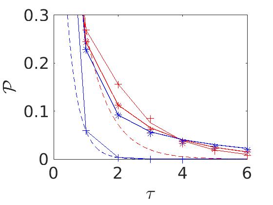
Figure 9: Survival probability $\mathcal{P}(\tau)$. The probability to find a pulse that has at least $\tau$ consecutive pulses at the same region. The red and blue colors refer respectively to survival in the red and in the blue regions. The $+$ symbols are for the time-independent $\theta{=}0$ Hamiltonian, and the $*$ symbols are for the Kepler-driven time dependent Hamiltonian. The solid lines are the analytic results based on the minimal stochastic model (the thicker lines are for the Kepler-driven Hamiltonian). The dashed lines illustrate the naive exponential decay for the time-independent $\theta{=}0$ Hamiltonian.

V Minimal stochastic model

The failure of $P_{n,m}$ to reproduce $\mathcal{P}(\tau)$ is easily understood by inspection of phase space. For presentation purpose we focus on the stickiness in the “red” region(s) of Fig. ​​6. Regarding this region as composed of tiny phase space cells, we can determine what is the “survival time” in the red region for each cell. Then we realize that red cells with large survival time constitute a minority. Accordingly, $P_{n,m}$ should be regarded as the coarse-graining of a finer kernel $P_{\nu,\mu}$. Note that the type of index (Roman vs Greek) is used in order to distinguish the coarse-grained version from the “microscopic” version.

We would like to construct a minimal version for $P_{\nu,\mu}$, that corresponds to $P_{n,m}$, such that $\mathcal{P}(\tau)$ is reproduced correctly. Using this model we would like to relate the rate of spreading to the stickiness. The calculation of $\mathcal{P}(\tau)$, given a Markov kernel $\bm{P}$, is done as follows:

$$\mathcal{P}(\tau)\Big{|}_{\text{Markov}}\ \ =\ \ \left(\frac{1}{\bm{p}^{{\dagger}}\bm{p}}\right)\bm{p}^{{\dagger}}(\bm{Q}\bm{P})^{\tau}\bm{p}$$ (8)

In this expression $\bm{p}$ is a vector that contains the initial distribution within the bins. Specifically, we assume uniform distribution within the “red” bins. Note that $(\bm{p}^{{\dagger}}\bm{p})^{-1}$ is the number of participating red bins. The matrix $\bm{Q}$ is a projector on the red bins, and the final projection provides the total survival probability after $\tau$ iterations with $\bm{Q}\bm{P}$. We can adopt the area of $\mathcal{P}(\tau)$ as a measure for stickiness. For a given Markov process it is calculated as follows:

$$\mathcal{S}=\sum_{\tau}\mathcal{P}(\tau)=\left(\frac{1}{\bm{p}^{{\dagger}}\bm{p}}\right)\bm{p}^{{\dagger}}\left[\frac{1}{1-\bm{Q}\bm{P}}\right]\bm{p}\ \ \ \ \ \ \$$ (9)

Note that the naive expression Eq. ​​(7) gives a rather low value ${\mathcal{S}=1/(1-P_{s})}$.

We already saw in Fig. ​​9 that a naive 2-region model is not enough to reproduce the stickiness. So the minimum is apparently 3-regions. We assume that we have $n_{0}$ phase space cells in the non-red region, and $n_{1}+n_{2}$ cells in the red region. Consider the possibility of fully-connected chaos with ${N=n_{0}+n_{1}+n_{2}}$ cells with equal transition probabilities. Then the reduced $\bm{P}$ that describes the transitions of probabilities between the 3 regions would be

$$\bm{P}=\frac{1}{N}\begin{pmatrix}n_{0}&n_{0}&n_{0}\\ n_{1}&n_{1}&n_{1}\\ n_{2}&n_{2}&n_{2}\end{pmatrix}$$ (10)

The survival probability in the red region would be ${P_{0}=(n_{1}+n_{2})/N}$, that is characterized by ${\mathcal{S}_{0}=1/(1-P_{0})}$.

We now turn to consider a mixed phase-space, where the chaotic sea is connected, but not fully-connected. Specifically, we assume that the transition probabilities from the $n_{0}$ cells to the $n_{1}$ cells are all equal to $p_{1}$, while all the transition probabilities between the $n_{1}$ cells and the $n_{2}$ cells equal $q$. Then the reduced $\bm{P}$ that describes the transitions of probabilities between the 3 regions is

$$\bm{P}=\begin{pmatrix}1-n_{1}p_{1}&n_{0}p_{1}&0\\ n_{1}p_{1}&1-n_{0}p_{1}-n_{2}q&n_{1}q\\ 0&n_{2}q&1-n_{1}q\end{pmatrix}$$ (11)

The model is characterized by 4 parameters

$$P_{0}\ = \ \frac{(n_{1}+n_{2})}{n_{0}+(n_{1}+n_{2})}\ \ \equiv\ \ \frac{N_{\text{red}}}{N}$$ (12)

$$R_{s}\ = \ \frac{n_{2}}{n_{1}}$$ (13)

$$P_{s}\ = \ 1-\left(\frac{n_{1}}{n_{1}+n_{2}}\right)n_{0}p_{1}$$ (14)

$$Q_{s}\ = \ n_{1}q$$ (15)

The parameters $P_{0}$ and $R_{s}$ reflect the relative size of the regions. Namely, $P_{0}$ is the relative size of the red region (and hence would equal the survival probability in the red region if we had fully connected chaos), and $R_{s}$ is fraction of sticky red cells. The parameters $P_{s}$ and $Q_{s}$ reflect the transitions between the regions. We could have added also direct transitions with probability $p_{2}$ between the $n_{0}$ and the $n_{2}$ cells, but it turns out that this would be a redundancy for our purpose. Also the total number of cells is insignificant for the analysis.

All the probabilities in the $\bm{P}$ matrix must be less than $1$. This imposes some constraints over the valid range of the model parameters. In particular one realizes that if ${R_{s}>1}$ then ${P_{s}>(1/2)}$. Therefore, in order to describe a model that exhibits stickiness (small $P_{s}$) we have to assume ${R_{s}<1}$, and then the same constraints imply that ${P_{s}>[R_{s}/(R_{s}+1)]}$.

In practice the effective parameters ${(P_{s},R_{s},Q_{s})}$ are determined from $\mathcal{P}(\tau)$, as explained in Appendix D. These parameters determine the stickiness measure of Eq. ​​(9), namely,

$$\mathcal{S}\ \ =\ \ \frac{1}{1{-}P_{s}}+\left[\frac{R_{s}}{R_{s}+1}\right]\frac{1}{Q_{s}}$$ (16)

For ${R_{s}=0}$ we get the naive result ${\mathcal{S}=1/(1-P_{s})}$. In the limit ${Q_{s}\rightarrow 0}$ there is no decay from the $n_{2}$ cells, and then the survival probability approaches $\mathcal{P}(\infty)=R_{s}/(1{+}R_{s})$, and $\mathcal{S}$ diverges. The minimal value ${\mathcal{S}=\mathcal{S}_{0}=1/(1{-}P_{0})}$ is obtained for a fully connected chaos.

On the basis of the simulations, we have determined $\mathcal{P}(\tau)$ for the blue and for the red regions, for both the $\theta{=}0$ Hamiltonian and for the Kepler-driven Hamiltonian. The results are displayed in Fig. ​​9. The effective model parameters have been extracted and are listed in Appendix D.

VI Stickiness and rate of spreading

We would like to relate the rate of spreading to the stickiness. Within the framework of the stochastic picture, the spreading is determined by the time dependent diffusion coefficient

$$D(t)\ \equiv\ \frac{1}{2}\sum_{\tau=-t}^{t}C(\tau)$$ (17)

with the correlation function

$$C(\tau)\ =\ \left\langle F_{\tau}F_{0}\right\rangle\ =\ \frac{1}{N}\sum_{\mu,\nu}f_{\mu}[\bm{P}^{\tau}]_{\mu,\nu}f_{\nu}$$ (18)

where $N$ is the number of cells, and $f_{\mu}$ is the $F$ value that is associated with the phase space cell that is indexed as $\mu$. Note that a finite result for $\mathcal{P}(\tau)$ is obtained provided ${\sum f_{\mu}=0}$, reflecting that the correlation function is defined after subtraction of the average (i.e. for a zero average signal).

Without the sticky red region, the correlation function is of the form $C(\tau)=C_{0}\delta_{\tau,0}$. With the red region included, we get correlations due the stickiness. To evaluate the contribution of the latter we use the reduced matrix of Eq. ​​(11), where all the cells are grouped into 3 regions. In such case the sum over $\mu$ in Eq. ​​(18) is replaced by a sum over regions, and the number of cells in each region should be introduced as a weight factor. Then one obtains

$$C(0)=C_{0}+P_{0}\mathcal{S}_{0}f_{\text{red}}^{2}$$ (19)

where $f_{\text{red}}$ is the average $F$ value of the red region, and it is implied that the average $F$ value of the non-red region is ${-P_{0}\mathcal{S}_{0}f_{\text{red}}}$. The summation over $\tau$ leads to Eq. ​​(18) with ${\bm{P}^{\tau}}$ replaced by ${1/(1-\bm{P})}$. The zero mode has to be excluded from the inversion. Including $C_{0}$ we get

$$\sum_{\tau=0}^{\infty}C(\tau)\ \ =\ \ C_{0}\ +\ P_{0}\mathcal{S}f_{\text{red}}^{2}$$ (20)

We define the correlation factor as follows:

$$c_{s}\ =\ \frac{\sum_{\tau}C(\tau)}{C(0)}\ =\ 2\left(\frac{\sum_{\tau=0}^{\infty}C(\tau)}{C(0)}\right)-1\ \ \ \$$ (21)

It is the correlation “time” in terms of iterations with the Poincaré map. For the minimal model of Eq. ​​(11) one obtains

$$c_{s}\ =\ 2\left(\frac{\mathcal{S}}{\mathcal{S}_{0}}\right)-1,\ \ \ \ \ \text{for $C_{0}{=}0$}$$ (22)

Note that for fully connected chaos we get $c_{s}=1$ as expected.

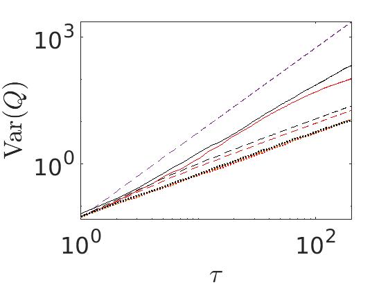
Figure 10: Stochastic modelling of spreading. The solid lines are $\text{Var}(Q)$ for the $F_{j}$ digitized sequences. See Appendix D for technical details regarding the ‘digitization’. Note that the “time” ($\tau)$ is the number of Poincaré steps. The red lines are for the $\theta{=}0$ Hamiltonian, and the black lines are for the Kepler-driven Hamiltonian. The lower dashed lines are the prediction of the effective stochastic model. The dotted lines are for a randomized $F_{j}$ sequence, namely, the expected result if the pulses were uncorrelated. The lower and upper dashed lines indicate $\propto t$ and $\propto t^{2}$ dependence (the former cannot be resolved from the dotted lines).

For the Kepler-driven system we observed an additional “blue” sticky region. Therefore we have to generalize the minimal model, such as to have two sticky regions, “red” and “blue”. The total number of cells is ${N=N_{0}+N_{\text{red}}+N_{\text{blue}}}$. We define ${P_{0}^{\text{red}}=N_{\text{red}}/N}$ and ${P_{0}^{\text{blue}}=N_{\text{blue}}/N}$. Each of the regions has its own $\mathcal{P}(\tau)$, with effective parameters that have been determined in Appendix D. The implied average $F$ value of the $N_{0}$ region is ${f_{0}=-(1/N_{0})[N_{\text{red}}f_{\text{red}}+N_{\text{blue}}f_{\text{blue}}]}$. Then one obtains

$$C(0)=C_{0}+\frac{N_{0}}{N}f_{0}^{2}+P_{0}^{\text{red}}f_{\text{red}}^{2}+P_{0}^{\text{blue}}f_{\text{blue}}^{2}\ \ \ \ \$$ (23)

and

$$\sum_{\tau=0}^{\infty}C(\tau)\ =\ C_{0}+P_{0}^{\text{red}}\mathcal{S}^{\text{red}}f_{\text{red}}^{2}+P_{0}^{\text{blue}}\mathcal{S}^{\text{blue}}f_{\text{blue}}^{2}\ \ \ \$$ (24)

For $N_{\text{blue}}=0$ these equations lead back to Eq. ​​(22).

The correlation factor can be extract numerically from the $S_{Q}$ plots of Fig. ​​4. Namely, it is the ratio between the slope of $S_{Q}^{2}$ for the true pulse sequence, and that of the randomized sequence (of the same pulses). By inspection of Fig. ​​10 we see that the true $S_{Q}^{2}$ exhibits a super-diffusive transient, indicating long-time correlations that are not captured by our simplified model. The agreement with the minimal model is qualitative rather than quantitative. Some extra details about the quantitative aspect are provided in Appendix D.

We see that a model that faithfully reproduces $\mathcal{P}(\tau)$ is not enough for the determination of $C(\tau)$. In principle we could have introduced a more elaborated stochastic model, that features a hierarchy of red and blue regions, but such an approach has no practical value, and does not allow the derivation of analytical results.

VII Cycle vs Modulation

It is important to distinguish between Cycle and Modulation. Consider an Hamiltonian $H_{\bm{R}}$ where $\bm{R}$ is a set of control parameters. In a time dependent scenario, we can say that the Hamiltonian varies along a curve in a parametric manifold. A modulation can be parametrized by a single non-cyclic parameter, say $R(t)=A\cos(\Omega t)$, while a cycle requires an angle parameter, say ${\theta(t)=\Omega t}$, where $\theta$ is defined modulo $2\pi$. A prototype example for cyclic driving is presented in Fig. ​​11.

It is sometimes difficult to determine whether the time dependence in the Hamiltonian should be regarded as Constant or as Modulated or as Cyclic driving. For example: the time dependence for particle in a rotating box can be removed by transforming into a rotating frame. Similarly, the time dependence for a particle in an expanding box can be removed via a dilation transformation. In the case of a cycle, the outcome depends in general on the sense of the cycle, and furthermore, for a mixed phase space, we expect difference in the rate of spreading.

At first glance, one may naively think that a Kepler-driven system qualifies as Cyclic driving. The two parameters might be $(X(t),Y(t))$ or equivalently $(\mathsf{R}(\theta),\mathsf{K}(\theta))$ as in Eq. ​​(1). But it turns out that for a proper Kepler driving the cycle degenerates into a modulation. In order to avoid such ‘degeneracy’, we have to assume an asymmetric $\mathsf{R}(\theta)$, for example ${\mathsf{R}(\theta)\propto[1+\varepsilon\cos(\theta)+\varepsilon^{\prime}\sin(2\theta)]^{-1}}$, that is illustrated in Fig. ​​12.

If we have a non-degenerate cycle, we can ask whether the rate of spreading depends on its sense (cycle vs reversed cycle). For a system with mixed-chaotic phase space indeed we can have such dependence, as discussed for e.g. the mushroom billiard in [11]. A different illustration of the same idea is provided in Fig. ​​11. During the cycle the space is divided by a barrier (that serves as a “valve”) into two regions. This is done periodically, and out-of-phase with respect to the piston movement. Specifically, in the plotted illustration, the splitting ratio of the cloud is roughly 1:2 for forward cycle, and roughly 1:1 for reversed cycle. Changes of energy due to changes in the volume obey a simple “ideal gas” multiplicative law ${E\mapsto\alpha E}$, where $\alpha$ is given by Eq. ​​(56). The value of $\alpha$ depends on the sense of the cycle, due to the different splitting ratio, and we get ${\alpha=10/9}$ and ${\alpha=9/8}$ respectively.

Figure 11: The billiard paradigm. This caricature clarifies the mechanism of dissipation in the quasi-static limit. The control parameters are ${\bm{R}=(X,W)}$, where $X$ is the position of the piston, and $W$ is the height of a dividing barrier. Consider the “blue” quasi-static cycle: The barrier is turned on ($W=\infty$); The piston is pushed in; The barrier is turned off ($W=0$); The piston is pushed out. Such cycle, unlike the “red” modulation, raises the average energy of the system (${E\mapsto\alpha E}$ with ${\alpha>1}$). Note that the blue and red $E(t)$ plots reflect the average over an ensemble of trajectories.

However, the billiard examples are rather artificial. They are based on construction that allows a sharp distinction between regions in (phase)space. Generic systems, such as the Hill’s Hamiltonian, do not feature dramatic splitting and merging of well defined (phase)space regions. Consequently, dependence on the sense of the cycle is not a prominent effect, and careful numerical procedure is required to detect it. This motivates the following discussion of directionality dependence.

Directionality.– The dependence on the sense of the cycle is related to the directionality dependence of a modulation. The argument is as follows: A modulation can be encoded by a sequence $A\bar{A}A\bar{A}\cdots A\bar{A}\cdots$. The inverse modulation is clearly the same sequence. A cycle can be encoded as $A\bar{B}A\bar{B}\cdots A\bar{B}\cdots$. The reversed cycle $B\bar{A}B\bar{A}\cdots B\bar{A}\cdots$ is distinct if the cycle is not degenerated (${A\neq B}$), and provided $A$ and $\bar{A}$ are not characterized by the same spreading rate. It is therefore enough to establish dependence on directionality.

Regarding the sequence $F_{j}$ as a ‘signal’, we ask whether it looks statistically the same during the ‘forward’ half period when $R(\theta)$ changes from $R(0)$ to $R(\pi)$, and the ‘backward’ half period when it changes from $R(\pi)$ to $R(0)$. In the standard paradigm of quasi-static processes the directionality has no significance. In Fig. ​​13 we plot the distribution of the $F$ values for the two groups of pulses. For the full signal the distribution of the $F_{j}$ over the bin is uniform by definition. But if we look only on the pulses that belong to the ‘backward’ half-periods we see that the small values (blue pulses) become slightly more frequent, as opposed to the large values (red pulses) that become slightly less frequent. The difference is very small. Still, it indicates that the steady state is not the same for “forward” and “backward” driving.

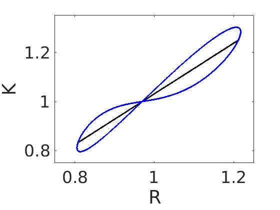
Figure 12: Cyclic driving. An example for a generic driving cycle in ${(\mathsf{R},\mathsf{K})}$ is illustrated by the blue line, where ${\mathsf{R}(\theta)\propto[1+\varepsilon\cos(\theta)+\varepsilon^{\prime}\sin(2\theta)]^{-1}}$, and $\mathsf{K}$ is determined by Eq. ​​(2), with $\varepsilon{=}0.2$ and $\varepsilon^{\prime}{=}0.1$. For Kepler driving we set $\varepsilon^{\prime}{=}0$ and get the black line, which is a single-parameter modulation.

Figure 13: Directionality dependence. The probability distribution of the $F_{j}$ over the bins is uniform by definition. It can be regarded as the sum of ‘forward’ pulses distribution, and ‘backward’ pulses distribution. Here we plot the deviation of the cumulative probability distribution of the backward pulses, from a uniform distribution. The horizontal axis is the indexed $F$ value (smallest value is indexed as 1, largest value is indexed as 38516). We see that the small values (blue pulses) become slightly more frequent, as opposed to the large values (red pulses) that become slightly less frequent.

VIII Dissipation

Dissipation is associated with energy spreading. The standard theory [2, 3, 4] assumes a globally chaotic energy surface that instantly ergodizes at any moment. It follows that the phase-space volume $\mathcal{N}(E;\theta)$ is an adiabatic invariant, where $\theta(t)$ is a slowly varying control parameter. For a closed cycle, the conservative work is zero. Still, beyond the zero-order adiabatic result, there is diffusion in energy with coefficient ${D_{E}=\nu\dot{\theta}^{2}}$, where $\nu$ is the intensity of the fluctuations, i.e. the algebraic area of $C(t)$. From the Fokker-Plank description of the spreading process, one deduces the rate of absorption ${\dot{E}=\mu\dot{\theta}^{2}}$, aka the Kubo formula, with dissipation coefficient $\mu$ that is related to $\nu$ via a fluctuation-dissipation relation [5, 6, 7, 8], namely ${\mu=(1/2)\beta\nu}$, where $\beta(E)$ is some version of microcanonical inverse temperature, as defined in Appendix E. Consequently, for periodic driving with frequency ${\Omega\equiv\dot{\theta}}$ one expects an amount ${Q=2\pi\mu\Omega}$ of dissipated energy per cycle, which vanishes in the quasi-static limit (${\Omega\rightarrow 0}$).

For a driven mixed-chaotic system, we expect parametric dissipation, meaning that the dissipated energy per cycle (${Q}$) approaches a finite non-zero constant in the limit $(\Omega\rightarrow 0)$, and depends on the directionality of the driving as discussed in the previous paragraph. Billiard examples that have been discussed in the past, as well as that of Fig. ​​11, are illuminating, but do not fully reflect some complications that are encountered once we deal with a generic system, such as Hill’s. In what follows we highlight those zero-order subtleties, and also generalize the first-order formulation.

Zero order dissipation.– In systems with mixed-chaotic dynamics, we can get irreversibility due to phase space spreading (aka growth of the entropy), as well as dissipation (growth of the average energy), even in the quasi-static limit. The derivation of this claim requires phase-space generalization of [11]. This generalization is presented in Appendix E. We write the phase space area as ${\mathcal{A}=\sum_{\mu}\mathcal{A}_{\mu}}$, where ${\mu}$ distinguishes different regions. Each region might have a different “inverse temperature” ${\beta_{\mu}}$. Then we obtain the following result:

$$\left\langle Q\right\rangle_{0}\ \ \approx \ \ -\sum_{steps}\sum_{\mu}\frac{\delta\mathcal{A}_{\mu}}{\beta_{\mu}\mathcal{A}}+\mathcal{O}(\delta\mathcal{A}^{2})$$ (25)

This expression is obtained from Eq. ​​(55) after expansion with respect to ${\delta\mathcal{A}=\mathcal{A}_{\mu}-\mathcal{A}_{\mu}^{(0)}}$. Based on Eq. ​​(25) our observation is that we can get an $\mathcal{O}(\delta\mathcal{A})$ non-zero result provided the $\beta_{\mu}$ are non-identical. In such case $\left\langle Q\right\rangle_{0}$ can switch sign for a reversed cycle. This should be contrasted with a Billiard system for which the ${\beta_{\mu}=1/E}$ are identical, and $\left\langle Q\right\rangle_{0}$ is always positive.

First order Dissipation.– We define ${\mathcal{F}=-\partial\mathcal{H}/\partial\theta}$. For a periodically driven Hamiltonian with ${\dot{\theta}=\Omega}$ we have ${\dot{E}=-\Omega\mathcal{F}(t)}$. Integrating over a cycle, squaring, and averaging over an ensemble, we get ${\text{Var}(Q)=2\pi\nu\Omega}$, where $\nu$ is the intensity of the fluctuations (the area of the $\mathcal{F}$ autocorrelation function). This assumes a globally chaotic energy surface. If we have a fragmented phase-space (as in the previous Billiard example) we get ${\text{Var}(Q)=\text{Var}_{0}(Q)+2\pi\nu\Omega}$, where $\text{Var}_{0}(Q)$ is the variance that is associated with $\left\langle Q\right\rangle_{0}$. Using the above explained fluctuation-dissipation reasoning we deduce that the energy increase per cycle is

$$\left\langle Q\right\rangle\ \ =\ \ \left\langle Q\right\rangle_{0}\ +\ \frac{1}{2}\beta_{\text{eff}}\left[\text{Var}_{0}(Q)+2\pi\nu\Omega\right]$$ (26)

This expression goes beyond Kubo, because the zero order spreading is taken into account. Note that if correlations persist over a time duration that is longer than a cycle, the result is a long super-diffusive transient as in Fig. ​​4. In any case the appropriate correlation factor $c_{s}$ has to be incorporated in the calculation of ${\nu}$, as discussed in Sec. (VI).

IX Summary and outlook

We have introduced an effective stochastic theory for quasi-static spreading in systems with mixed chaotic phase space. The main objective was to provide tools for the analysis of phase space spreading. More specifically, the spreading of the energy, which is useful for the calculation of the average energy growth (dissipation), and possibly for estimating the rate of “evaporation”.

For demonstration of our approach we have selected Hill’s Hamiltonian. This toy model, by itself, has physical significance, as discussed in the Introduction. The problem of interest has possibly direct relevance to studies that concern the long-term stability of planets in binary systems [44, 45, 46]. Furthermore, it illuminates the relevance of mixed-chaotic dynamics in the context of the 3 body problem. The model has all the essential ingredients for our analysis. However, in retrospective, we have to admit that stickiness, rather than a zero-order dissipation effect, is the dominant feature that determines the rate of spreading. This stands in contrast to the analysis of energy spreading due to quasi-static driving of specially-designed Billiard systems [9, 10, 11], that has motivated the present study.

Our agenda was, on the one hand, to characterize the multi-dimensional phase space dynamics via “signal-analysis” of a single chaotic trajectory. On the other hand, we wanted to reproduce the essential statistical features of the ‘signal’ using a minimal Markovian model.

For the characterization of the chaotic motion, we represent the chaotic trajectory as a Poincaré sequence of pulses ($F_{j}$). The value of $F$ is regarded as a ‘radial’ phase space coordinate, that is used in order to divide phase space into regions (indexed by $n$). We realize that this coarse-graining is too rough: we cannot build on it a Markov process that reproduces the observed stickiness. We therefore have to define a refined version of the Markov process that reflects the hierarchic structure of phase space. Consequently, we constructed a minimal model that allows to reproduce the observed stickiness. This model suggests a relation between the stickiness and the enhancement that is observed is the rate of spreading. Unfortunately, in the present model, the quantitative agreement is poor due to long range correlations that were neglected.

Specifically, for the frozen dynamics, we have identified stickiness in peripheral regions of the chaotic sea. A minimal stochastic model for such configuration requires 3 regions (central chaotic region; non-sticky peripheral chaotic region; sticky peripheral chaotic region). Surprisingly in the Kepler-driven system extra stickiness manifests in the native chaotic sea. This extra stickiness is related to the appearance of an additional “swamp chaotic region”, where chaos penetrates due to the time-dependence of the Hamiltonian. Nevertheless, it can be treated on equal footing using the same stochastic model (with extra regions).

We also looked for directionality dependence, implying that the rate of spreading is not the same if a cycle is reversed. We have clarified that also this effect can be identified from the “signal analysis” of the Poincaré sequence. For the model system that we have studied, the finding was that it is a very weak effect (a few percent difference).

Finally, for sake of generality, we have explained how the Kubo theory of dissipation can be generalized in order to incorporate both the zero-order and first-order irreversibility. This picture implies exponential energy growth if $\left\langle Q\right\rangle$ of Eq. ​​(26) is proportion to $E$. This is indeed the case for Billiard systems if ${\left\langle Q\right\rangle_{0}\neq 0}$ as discussed originally by [9, 10, 11]. More generally we can get from Eq. ​​(26) different energy dependence, say ${\dot{E}=\lambda E^{\alpha}}$. Note that for ${\alpha>1}$ one obtains hyperbolic-like growth that leads to escape ${E\sim 1/(t-t_{e})^{1/(\alpha-1)}}$ within a finite time $t_{e}$. The exploration of such scenario requires further study of possibly different model systems.

Appendix A Basic formulas for Kepler motion

The constant of motion in Kepler problem is the angular momentum. In terms of polar coordinates $(\theta,R)$ we define ${\ell=R^{2}\dot{\theta}}$. Kepler’s area law is the statement

$$\frac{d}{dt}\text{Area}=\frac{1}{2}\ell$$ (27)

The Kepler motion is along an ellipse with major axes ${a}$ and ${b=\sqrt{1-\varepsilon^{2}}a}$. We also define ${c=\sqrt{ab}}$. From the area law it follows that ${T=2\pi ab/\ell}$. Accordingly the frequency is ${\Omega=\ell/(ab)}$. So we have the relation

$$\ell\ \ =\ \ ab\Omega\ \ =\ \ c^{2}\Omega$$ (28)

For a circular motion of radius $R{=}a{=}b{=}c$, the frequency the motion is determined by the equation

$$\Omega^{2}a^{3}=G(M_{1}+M_{2})\equiv GM$$ (29)

This result applies also if the motion is along an ellipse. The equation of the ellipse is

$$R(\theta)\ \ =\ \ \frac{(1-\varepsilon^{2})\,a}{1+\varepsilon\cos(\theta)}\ \ \equiv\ \ c\mathsf{R}(\theta)$$ (30)

Note that with this definition $\mathsf{R}(\theta)$ is square-normalized to unity. The equation of motion for the radial motion is

$$\ddot{R}=\frac{\ell^{2}}{R^{3}}-\frac{GM}{R^{2}}$$ (31)

which implies conservation of energy (here we are in the non-rotating “lab” frame):

$$E\ =\ \frac{1}{2}\dot{R}^{2}+\frac{\ell^{2}}{2R^{2}}-\frac{GM}{R}\ =\ -\frac{1}{2}a^{2}\Omega^{2}$$ (32)

Given $(GM,E,\ell)$, the orbit, up to orientation, is described by $(\Omega,a,c)$. The $\Omega$ and the $a$ are determined by Eq. ​​(29) and Eq. ​​(32), while $c$ is determined by Eq. ​​(28), and we have the ratio ${c/a=(1-\varepsilon^{2})^{1/4}}$.

Appendix B The generalized Hill Hamiltonian

We use the notations ${\bm{r}=(x,y)}$ and ${\bm{p}=(p_{x},p_{y})}$. We consider time dependent $R(t)$ and $\theta(t)$. Without loss of generality, we set $\mathsf{m}{=}1$ for the mass of the satellite. The Hamiltonian is:

$$\mathcal{H}\ \ =\ \ \frac{1}{2}\bm{p}^{2}\ +\ U(\bm{r};R(t),\theta(t))$$ (33)

In order to transform the Hamiltonian we use a sequence of canonical transformations. For clarity we use below “quantum language”. Given a transformation $T=\exp[-i\alpha(t)G]$ that is generated by $G$, we use below the formula

$$\mathcal{H}\ \ = \ \ T^{{\dagger}}\mathcal{H}T-iT^{{\dagger}}\frac{\partial T}{\partial t}$$ (34)

$$= \ \ T^{{\dagger}}\mathcal{H}T-\dot{\alpha}G$$ (35)

The first transformation is to a rotating reference frame with ${T=\exp[-i\theta(t)L]}$ where ${L=\bm{r}\wedge\bm{p}=xp_{y}-xp_{y}}$

$$\mathcal{H}=\frac{1}{2}\bm{p}^{2}-\dot{\theta}L+U(\bm{r};R(t),0)$$ (36)

The second transformation is a time dependent dilation with ${T=\exp[-i(\ln R)K]}$ where ${K=\bm{r}\cdot\bm{p}=xp_{x}+yp_{y}}$. Note that ${T^{{\dagger}}xT=Rx}$ and ${T^{{\dagger}}pT=(1/R)p}$. Using the notation ${U(r)=U(r;1,0)}$ we get

$$\mathcal{H} = \frac{1}{2R^{2}}\bm{p}^{2}-\frac{\dot{R}}{R}K-\dot{\theta}L+\frac{1}{R}U(\bm{r})$$ (37)

$$= \frac{1}{2R^{2}}\bm{p}^{2}-\frac{\dot{R}}{R}\bm{r}\cdot\bm{p}-\dot{\theta}L+\frac{1}{R}U(\bm{r})$$ (38)

The third transformation is a time dependent Gauge with ${T=\exp[-i\Lambda]}$ where ${\Lambda=-(1/2)R\dot{R}r^{2}}$. Note that ${T^{{\dagger}}xT=x}$ and ${T^{{\dagger}}pT=p-\partial\Lambda}$. Accordingly we get

$$\mathcal{H} = \frac{1}{2R^{2}}(\bm{p}+R\dot{R}\bm{r})^{2}-\frac{\dot{R}}{R}\bm{r}\cdot(\bm{p}+R\dot{R}\bm{r})-\dot{\theta}L$$

$$+\frac{1}{R}U(\bm{r})+\frac{1}{2}[\dot{R}^{2}+R\ddot{R}]\bm{r}^{2}$$

$$= \frac{1}{2R^{2}}\bm{p}^{2}-\dot{\theta}L+\frac{1}{R}U(\bm{r})+\frac{1}{2}R\ddot{R}\bm{r}^{2}$$

$$= \frac{1}{2R^{2}}(\bm{p}-\bm{A})^{2}+\frac{1}{R}U(\bm{r})-\frac{1}{2}\left[R^{2}\dot{\theta}^{2}-R\ddot{R}\right]\bm{r}^{2}$$

where ${\bm{A}=R^{2}\dot{\theta}\bm{r}_{\perp}}$ with ${\bm{r}_{\perp}=(-y,x)}$. Given $R(t)$ and $\theta(t)$, the above Hamiltonian can be written schematically as

$$\mathcal{H}(\bm{r},\bm{p};\,\theta(t),R(t))\ \ =\ \$$

$$\frac{1}{R(t)^{2}}\left\{\frac{1}{2}(\bm{p}-\ell(t)\bm{r}_{\perp})^{2}+R(t)U(\bm{r})-\frac{1}{2}K(t)\bm{r}^{2}\right\}$$

where $\ell(t)\equiv R^{2}\dot{\theta}$, and $K(t)\equiv(R^{2}\dot{\theta})^{2}-R^{3}\ddot{R}$. If we assume Kepler motion we get ${K(t)=\Omega^{2}a^{3}R(t)}$ from the radial equation of motion.

Appendix C Hamiltonian for a Kepler system

Due to the dilation transformation, the coordinate $r$ is dimensionless, and the distance between the stars is unity, while $p$ has the same units as $\ell$. We now assume that $\ell$ is constant for the cycles of interest. Consequently we can re-scale the momentum ${p:=\ell p}$. It is convenient to define the characteristic radius $c$ of the orbit through ${\ell\equiv\Omega c^{2}}$, where $\Omega$ is the frequency of the cycle. We also define the notation $R(t)=c\mathsf{R}(\theta(t))$. By definition of $c$ and from ${\dot{\theta}=\ell/R(t)^{2}}$ it follows that

$$\oint\left|\mathsf{R}(\theta)\right|^{2}\,\frac{d\theta}{2\pi}\ \ =\ \ 1$$ (39)

Given $\mathsf{R}(\theta)$ we have the identity

$$\frac{\ddot{\mathsf{R}}}{\Omega^{2}}\mathsf{R}^{3}\ \ =\ \ -\left(\frac{1}{\mathsf{R}}\right)^{\prime\prime}\mathsf{R}$$ (40)

where dot (^.) is for time derivative and prime (’) is for theta derivative.

We write the attraction constant between the satellite and the stars as $G_{0}M$, such that $U(r)=G_{0}Mu(r)$. The Hamiltonian takes the form

$$\mathcal{H}=\frac{\Omega}{\mathsf{R}^{2}}\left\{\frac{1}{2}(\bm{p}-\bm{r}_{\perp})^{2}+g\mathsf{R}u(\bm{r})-\frac{1}{2}\mathsf{K}\bm{r}^{2}\right\}\ \ \ \ \$$ (41)

where

$$\mathsf{K}\ =\ 1+\left(\frac{1}{\mathsf{R}}\right)^{\prime\prime}\mathsf{R}$$ (42)

and

$$g\ =\ \frac{G_{0}M}{c^{3}\Omega^{2}}\ \equiv\ \frac{\Omega_{0}^{2}}{\Omega^{2}}$$ (43)

For a Kepler driven system we use the notation

$$g_{\varepsilon}\ =\ \frac{GM}{c^{3}\Omega^{2}}\ =\ (1-\varepsilon^{2})^{-3/4}$$ (44)

and get the simpler Hamiltonian

$$\mathcal{H}=\frac{\Omega}{\mathsf{R}^{2}}\left\{\frac{1}{2}(\bm{p}-\bm{r}_{\perp})^{2}+\mathsf{R}\left(gu(\bm{r})-\frac{1}{2}g_{\varepsilon}\bm{r}^{2}\right)\right\}\ \ \ \$$ (45)

Given $\mathsf{R}(\theta)$ and $\Omega$ and $c$ we have ${\dot{\theta}=\Omega/\mathsf{R}^{2}}$. Consequently, if we use $\theta$ as time variable, we get the Hamiltonian Eq. ​​(45) without the $\Omega/\mathsf{R}^{2}$ term.

The simple minded slowness condition is ${\Omega\ll\Omega_{0}}$, which can be written as ${1\ll g}$. In analogy with the piston paradigm, we have to assure that ${\dot{R}\ll\dot{r}}$ where the typical velocity of the dust particles is ${\dot{r}\sim c\Omega_{0}}$. For Kepler motion, the maximum velocity of the “piston” is ${\dot{R}\sim c\epsilon g_{\epsilon}\Omega}$. Consequently, the slowness condition takes the form ${\varepsilon g_{\varepsilon}\ll g}$, which always breaks down if ${\varepsilon}$ is too close to unity.

Appendix D Determination of effective parameters

The $F_{j}$ values have been grouped into 10 bins. The pulses that belong to a given bin define a region $n$ in phase space. It is implied that the same number of pulses is associated with each region. In our jargon ${n=1}$ is the “blue” region and ${n=10}$ is the “red” region, and it is implied that for fully connected chaos the probability to stay in a red bin is ${P_{0}=0.1}$. The matrix $P_{n,m}$ of Fig. ​​8 characterizes the statistics of the transitions between regions. Additionally, we determine numerically the probability $\mathcal{P}(\tau)$ to stay in a given region as a function of $\tau$, see Fig. ​​9. Specifically, we have obtained $\mathcal{P}(\tau)$ for $[\theta{=}0,\text{red}]$, for $[\theta{=}0,\text{blue}]$, for $[\text{Kepler,red}]$, and for $[\text{Kepler,blue}]$. From that we have extracted (in each case) the staying probability ${P_{s}=\mathcal{P}(\tau{=}1)}$, and the stickiness measure $\mathcal{S}$. The latter is the ‘area’ of $\mathcal{P}(\tau)$. The additional effective parameters $(R_{s},Q_{s})$ are deduced via Eq. ​​(16), with value of $1/Q_{s}$ that fits the stretched tail of $\mathcal{P}(\tau)$. The results were respectively:

$$P_{s} = 0.27,0.06,0.24,0.23$$ (46)

$$R_{s} = 0.15,0.0003,0.092,0.067$$ (47)

$$Q_{s} = 0.65,0.83,0.42,0.26$$ (48)

$$\mathcal{S} = 1.57,1.06,1.52,1.53$$ (49)

The main difference between the Kepler-driven Hamiltonian and the frozen Hamiltonian is related to the stickiness in the blue region.

The ‘digitized’ signal is obtained as follows. We define $f_{n}$ as the average value that characterizes the $n$-th bin. Then we set ${\text{digitized}[F_{j}]=f_{n}}$, if $F_{j}$ belongs to the $n$-th bin. In order to analyze the stickiness-related correlations, we have regarded all the intermediate bins ($n=2\cdots 9$) as one region that is characterized by an average value $f_{0}$, while bins ${n=1,10}$ are characterized by $f_{\text{blue}}$ and $f_{\text{red}}$ respectively. Due to this digitization the noise is reduced by factor ${\sim 2.5}$. We are left with a signal that contains information that is related to the stickiness, and we can set ${C_{0}=0}$ in Eq. ​​(19). Consequently, this digitization procedure allows a meaningful comparison between the numerical results and the minimal model in Fig. ​​10.

The correlation factor $c_{s}$ can be extract numerically by inspection of Fig. ​​10. For the Kepler-driven system we get ${c_{s}=18}$, while for the $\theta{=}0$ Hamiltonian we get ${c_{s}=9}$. This is consistent with what we observed in Fig. ​​4. The minimal model does not take into account the observed long-time correlations, and therefore predicts much smaller values, namely, ${c_{s}=2.0}$ and ${c_{s}=1.7}$ respectively.

Appendix E Quasi-static energy spreading

The energy landscape of phase space is described by the function $E=\mathcal{H}(\bm{r},\bm{p};\theta)$. The $d\bm{r}d\bm{p}/(2\pi)^{\text{dof}}$ volume of an energy surface is denoted $\mathcal{N}(E;\theta)$, and corresponds to the number of phase space cells in semiclassical mechanics. The area of the energy surface is defined as ${\mathcal{A}(E;\theta)=\partial_{E}\mathcal{N}}$, and corresponds to the density of states. The microcanonical-like inverse temperature is $\beta=\partial_{E}\ln\mathcal{N}=\mathcal{A}/\mathcal{N}$. For a particle in a billiard of area $\mathcal{A}$, setting appropriate units for the mass, we get ${\mathcal{N}=\mathcal{A}E}$, and ${\beta=1/E}$. For a mixed phase space the total area is written as

$$\mathcal{A}(E;\theta)\ \equiv\ \partial_{E}\mathcal{N}\ =\ \sum_{\mu}\mathcal{A}_{\mu}(\theta)$$ (50)

This assumes that there is a way to identify distinct regions as in the billiard example of Fig. ​​11 where ${{\mu}=L,R}$ distinguishes the left and right regions, and $\mathcal{A}_{\mu}(\theta)$ is the respective geometric area of the ${\mu}$-th region, while $\theta$ is a parameter that is used to specify the position of the piston. Without any approximation we always have

$$\dot{E}\ =\ \left\langle\frac{\partial\mathcal{H}}{\partial\theta}\right\rangle_{t}\dot{\theta}\ \equiv\ -\Omega\mathcal{F}(\theta(t))$$ (51)

In the Ott-Wilkinson-Kubo formulation of linear response theory [2, 3, 4, 5, 6, 7, 8], it is assumed that for a quasi-static process the instantaneous average can be replaced by an evolving microcanonical average due to quasi-ergodicity. Accordingly, the variation of the energy becomes parameteric:

$$dE\ =\ \left\langle\frac{\partial\mathcal{H}}{\partial\theta}\right\rangle_{E,\theta}\!\!\!d\theta\ \ =\ \ -\left(\frac{\partial_{\theta}\mathcal{N}}{\partial_{E}\mathcal{N}}\right)d\theta$$ (52)

From the last relation it is implied that ${d\mathcal{N}=0}$, meaning that $\mathcal{N}(E;\theta)$ is an adiabatic invariant. With the definition of phase space area this can be written as

$$dE=-\frac{1}{\beta}\,[\partial_{\theta}\ln\mathcal{N}]\,d\theta\equiv-\frac{1}{\beta_{\text{eff}}}\,[\partial_{\theta}\ln\mathcal{A}]\,d\theta$$ (53)

where the latter equality defines $\beta_{\text{eff}}$. Adjusting notations to mixed phase space we write the change of the energy per-cycle as

$$dE\ =-\sum_{\mu}P_{\mu}(\theta)\frac{1}{\beta_{\mu}}\,[\partial_{\theta}\ln\mathcal{A}_{\mu}]\,d\theta$$ (54)

where $P_{\mu}(\theta)$ is the probability at region ${\mu}$ of the energy surface, and it is assumed that the regions are well defined. Ref [11] consider a more complicated case where the borders between regions is affected by $\theta$. But such complication does not affect the big picture.

For a Billiard system that undergoes a multi-step process of the type that is illustrated in Fig. ​​11, the dissipated energy per cycle is

$$\left\langle Q\right\rangle_{0}\ \ =\ \ -\frac{1}{\beta}\sum_{steps}\sum_{\mu}\frac{\mathcal{A}_{\mu}^{(0)}}{\mathcal{A}^{(0)}}\ln\left[\frac{\mathcal{A}_{\mu}}{\mathcal{A}_{\mu}^{(0)}}\right]$$ (55)

where $\beta=1/E$ assumes a narrow distribution around $E$. Here the outer summation is over steps of the cycle. We assume global chaos at transitions between steps. The superscript ”0” indicates the area at the beginning of a step. Without ”0” it is the area at the end of the step.

Billiard systems are simple enough to allow an improved (exact) version of Eq. ​​(55) that does not assume a narrow distribution around a fixed energy. Changes of energy due to changes in the volume obey the simple “ideal gas” multiplicative law ${E\mapsto\alpha E}$, with

$$\alpha\ \ =\ \ \sum_{steps}\sum_{\mu}\frac{(\mathcal{A}_{\mu}^{(0)})^{2}}{\mathcal{A}^{(0)}\mathcal{A}_{\mu}}$$ (56)

One can easily verify that $\left\langle Q\right\rangle_{0}$ of Eq. ​​(55) is consistent with $(\alpha-1)E$. Note that we always have ${\alpha>1}$.

Acknowledgment.– We thank Hagai Perets and Nicholas Stone for a helpful communication. This research was supported by the Israel Science Foundation (Grant No.283/18).

References

- [1] L.D. Landau, E.M. Lifshitz, Mechanics, 3rd. Ed., p. 154ff. Elsevier (1982).
- [2] E. Ott, Goodness of ergodic adiabatic invariants, Phys. Rev. Lett. 42, 1628 (1979)
- [3] R. Brown, E. Ott, C. Grebogi, Ergodic adiabatic invariants of chaotic systems, Phys. Rev. Lett, 59, 1173 (1987)
- [4] R. Brown, E. Ott, C. Grebogi, The goodness of ergodic adiabatic invariants J. Stat. Phys. 49, 511 (1987)
- [5] M. Wilkinson, A semiclassical sum rule for matrix elements of classically chaotic systems, J. Phys. A 20, 2415 (1987)
- [6] M. Wilkinson, Statistical aspects of dissipation by Landau-Zener transitions, J. Phys. A 21, 4021 (1988)
- [7] D. Cohen, Quantum Dissipation due to the interaction with chaotic degrees-of-freedom and the correspondence principle, Phys. Rev. Lett. 82, 4951 (1999)
- [8] D. Cohen, Chaos and Energy Spreading for Time-Dependent Hamiltonians, and the various Regimes in the Theory of Quantum Dissipation, Annals of Physics 283, 175-231 (2000)
- [9] V. Gelfreich, V. Rom-Kedar, K. Shah, D. Turaev, Robust Exponential Acceleration in Time-Dependent Billiards, Phys. Rev. Lett. 106, 074101 (2011)
- [10] T. Pereira, D. Turaev, Exponential energy growth in adiabatically changing Hamiltonian systems, Phys. Rev. E 91, 010901 (2015)
- [11] V. Gelfreich, V. Rom-Kedar, D. Turaev, Oscillating mushrooms: adiabatic theory for a non-ergodic system, JJ. Phys. A 47, 395101 (2015)
- [12] A. Dey, D. Cohen, A. Vardi, Adiabatic passage through chaos, Phys. Rev. Lett. 121, 250405 (2018)
- [13] R. Burkle, A. Vardi, D. Cohen, J.R. Anglin, Probabilistic hysteresis in isolated integrable and chaotic Hamiltonian systems, Phys. Rev. Lett. 123, 114101 (2019)
- [14] G. Arwas, D. Cohen, Monodromy and chaos for condensed bosons in optical lattices, Phys. Rev. A 99, 023625 (2019)
- [15] Y. Winsten, D. Cohen, Quasi-static transfer protocols for atomtronic superfluid circuits, Sci. Rep. 11, 3136 (2021)
- [16] G. M. Zaslavsky, M. Edelman, Hierarchical structures in the phase space and fractional kinetics, Chaos 10, 135 (2000)
- [17] G.M.Zaslavsky, Chaos, fractional kinetics, and anomalous transport, Physics Reports 371, 461 (2002)
- [18] S. Denisov, J. Klafter, M. Urbakh, Ballistic flights and random diffusion as building blocks for Hamiltonian kinetics, Phys. Rev. E 66, 046217 (2002)
- [19] R. Venegeroles, Universality of Algebraic Laws in Hamiltonian Systems, Phys. Rev. Lett. 102, 064101 (2009)
- [20] A. Sethi, S. Keshavamurthy, Driven coupled Morse oscillators: visualizing the phase space and characterizing the transport, Molecular Physics, 110, 717 (2012)
- [21] E.J. Mueller, Superfluidity and mean-field energy loops: Hysteretic behavior in Bose-Einstein condensates, Phys. Rev. A 66, 063603 (2002)
- [22] B. Wu and Q. Niu, Superfluidity of Bose–Einstein condensate in an optical lattice: Landau–Zener tunnelling and dynamical instability, New. J. Phys. 5, 104 (2003)
- [23] M. Machholm, C.J. Pethick, H. Smith, Band structure, elementary excitations, and stability of a Bose-Einstein condensate in a periodic potential, Phys. Rev. A 67, 053613 (2003)
- [24] O. Fialko, M.-C. Delattre, J. Brand, A.R. Kolovsky, Nucleation in Finite Topological Systems During Continuous Metastable Quantum Phase Transitions, Phys. Rev. Lett. 108, 250402 (2012)
- [25] S. Baharian, G. Baym, Bose-Einstein condensates in toroidal traps: Instabilities, swallow-tail loops, and self-trapping, Phys. Rev. A 87, 013619 (2013)
- [26] D. Dobbrott, J. M. Greene, Probability of Trapping-State Transition in a Toroidal Device, Phys. of Fluids 14, 7 (1971).
- [27] A. I. Neishtadt, Passage through a separatrix in a resonance problem with a slowly-varying parameter, J. Appl. Math. Mech. 39, 594-605 (1975).
- [28] A.V. Timofeev, On the constancy of an adiabatic invariant when the nature of the motion changes, JETP 48, 656 (1978).
- [29] J. Henrard, Capture into resonance: an extension of the use of adiabatic invariants, Celestial Mechanics 27, 3-22 (1982).
- [30] J.R. Cary, J. R., D.F. Escande, J.L. Tennyson, Adiabatic-invariant change due to separatrix crossing, Phys. Rev. A 34, 4256–4275 (1986).
- [31] J.H Hannay, Accuracy loss of action invariance in adiabatic change of a one-freedom Hamiltonian, J. Phys. A 19, L1067–L1072 (1986).
- [32] J.R. Cary, R.T. Skodje, Reaction probability for sequential separatrix crossings, Phys. Rev. Lett. 61, 1795–1798 (1991).
- [33] A.I. Neishtadt, Probability phenomena due to separatrix crossing, Chaos 1, 42 (1991).
- [34] Y. Elskens, D.F. Escande, Slowly pulsating separatrices sweep homoclinic tangles where islands must be small: an extension of classical adiabatic theory, Nonlinearity 4, 615–667 (1991).
- [35] T. Eichmann, E.P. Thesing, J.R. Anglin, Engineering separatrix volume as a control technique for dynamical transitions. Phys. Rev. E 98, 052216 (2018)
- [36] A. Neishtadt, On mechanisms of destruction of adiabatic invariance in slow–fast Hamiltonian systems, Nonlinearity 32 (11), R53 (2019).
- [37] R. Burkle, A. Vardi, D. Cohen, J.R. Anglin, How to probe the microscopic onset of irreversibility with ultracold atoms, Scientific Reports 9, 14169 (2019)
- [38] O. Morsch, M. Oberthaler, Dynamics of Bose-Einstein condensates in optical lattices, Rev. Mod. Phys. 78, 179 (2006).
- [39] I. Bloch, J. Dalibard, W. Zwerger, Many-body physics with ultracold gases, Rev. Mod. Phys. 80, 885 (2008).
- [40] A. R. Kolovsky, Bose-Hubbard hamiltonian: Quantum chaos approach, Int. J. Mod. Phys. B 30, 1630009 (2016).
- [41] V. Szebehely, Theory of Orbits: The Restricted Problem of Three Bodies, Academic Press (May 13, 2013).
- [42] W.S. Koon, M.W. Lo, J.E. Marsden, S.D. Ross, Dynamical Systems, the Three-Body Problem and Space Mission Design, Marsden Books (2008).
- [43] K. Meyer, G. Hall, D. Offin, Introduction to Hamiltonian Dynamical Systems and the 3-Body Problem, Springer (2008).
- [44] M.J. Holman, P.A. Wiegert, Long-Term Stability of Planets in Binary Systems, The Astronomical Journal 117, 621 (1999)
- [45] Z.E. Musielak, M. Cuntz, E.A. Marshall, and T.D. Stuit, Stability of planetary orbits in binary systems, A&A 434, 355 (2005)
- [46] G. De Cesare, R. Capuzzo-Dolcetta, On the stability of planetary orbits in binary star systems Astrophysics and Space Science 366, 53 (2021)
- [47] N.C. Stone, N.W.C. Leigh, A statistical solution to the chaotic, non-hierarchical three-body problem, Nature 576, 406 (2019)
- [48] Y. Barry Ginat, H.B. Perets, Analytical, Statistical Approximate Solution of Dissipative and Nondissipative Binary-Single Stellar Encounters, Phys. Rev. X 11, 031020 (2021)