Evolution of Cluster of Stars in $f(R)$ Gravity

Abstract

This paper explores the dynamics of evolving cluster of stars in the presences of exotic matter. The $f(R)$ theory is used to presume exotic terms for evolution scenario. We use structure scalars as evolution parameters to explore dynamics of spherically symmetric distribution of evolving cluster of stars. We consider Starobinsky model, $f(R)=R+\epsilon R^{2}$ and study different evolution modes having features like isotropic pressure, density homogeneity, homologous and geodesic behavior. It is concluded that dynamics of these modes of evolution depends upon the behavior of dark matter. The presences of dark matter directly affects the features of cluster like anisotropic pressure, dissipation, expansion, shear as well as density homogeneity. The evolution having homogeneous density and isotropic pressure depends upon conformally flat and non-dissipative behavior of baryonic as well as non baryonic matter. The dissipation factor induces density inhomogeneity in the expanding clusters having shear effects. The non dissipative homologous evolution also be discussed in the presence and absence of shear effects. It is found that high curvature geometry in the presence of shear supports homologous evolution. Expanding clusters are also explored in the presences of dissipation of dark matter and shear effects. By using quasi-homologous conditions the geodesic evolution is studied. It is theoretically showed that geodesic and homologous conditions depends upon each other. Finally we investigate behavior of Starobinsky model for a stellar structure $4U1820-30$ toward center. It is found that for increasing values of $\epsilon$ the DM behavior is dominant as compare to baryonic matter.

Keywords: $f(R)$ Theory; Dark Matter; Cluster of Stars.
PACS: 04.40.Dg; 04.50.Kd; 98.65.-r; 98.65.Cw.

1 Introduction

The mystery of dark energy and dark matter is one of the important topic of modern physics. Recently, Planck’s [1] gives distribution which shows $5\%$ baryonic matter with $27\%$ dark matter (DM) and $71\%$ dark energy (DE). It is believed that DE is responsible for the expansion of the universe in accelerated rate as time is passing. The matter that can be seen easily is known as baryonic matter. While the DM or non-baryonic matter is an invisible hypothetical type of matter which does not or very weakly interact with electromagnetic radiations. The DM is observable by its gravitational effects on baryonic matter. Since the rise of last century, a sensational amount of evidence indicating a dominant contribution of DM to the universe. Different detection mechanism have been constructed to study the nature of DM. Among these, the search for appearing of DM in stellar bodies comes as inexpensive and ingenious detection strategy. Naturally, in this context, most indirect searches have been focused yielding fruitful results that are complementary and competitive.

In order to explore mystery of dark universe (DE and DM) many candidates are introduced by researchers. In this context, the $f(R)$ theory of gravity [2] is one of the most explored example involving higher order curvature terms. This theory is the generalization of Einstein Hilbert action with a generic function of curvature ($f(R)$). The $f(R)$ gravity is very interesting because of its higher order curvature terms, which can represents both DE and DM problems sufficiently. Many researchers [3, 4] used various $f(R)$ models to study the effects of DE and DM. The Starobinsky model ($f(R)=R+\epsilon R^{2}$) [5, 6] is a model of gravity in power-law type of the Ricci scalar that has efficiently promoted the early-time cosmic expansion and DM issues.

A stars cluster is a group of stars which are gravitationally bound together. The average stars distance in a cluster is much closer than average distance between stance and rest of the galaxy. It is believed that study of stars cluster can be used to examine the evolution and formation of galaxies. This in turn describes evolution and formation of the galactic system. There have been a meaningful theoretical efforts to study the evolution and formation of stars cluster [7]. In this context, it would be interesting to discuss the evolution of stars cluster through the technique of structure scalars.

Structure scalars are scalar expressions which deals with mixture of physical terms like density, anisotropy of pressure as well as Weyl tensor. These scalars are used to describe the evolution of self-gravitating systems. Firstly, Herrera et al. [8] suggested the orthogonal division of the Riemann curvature tensor and found several scalars of structure. The basic properties of stellar are then correlated with these scalars. By using structure scalars, they interpret some properties of relativistic structures. They studied hydrodynamics along with thermodynamics of self-gravitating systems like Lemaitre-Tolman-Bondi space time [9], spherical model with electric charge and cosmological constant [10], cylindrically as well as axially symmetric self-gravitating systems [11]. Herrera et al. [12] discussed evolution of complex less stellar systems based on baryonic matter with the help of structure scalars. In modified theories, Sharif and Manzoor [13] and Yousaf and his collaborators [14] applied these findings to different cosmic models.

The DM is an important ingredient of the cluster of stars [15]. It is well known about $95\%$ of the total mass of the stars cluster is made up of DM. The problems of galactic clusters, galactic rotational curves and the mass discrepancy indicate the importance and existence of DM in the evolution of stars cluster [16]. It is believed that the presence of DM affects the stellar evolution. So the study of evolving stellar like clusters in the presence of DM may determinate the dynamics of its evolving process. In this way, we may get about modifications that are not visible in the structure of the universe [13, 17]. In the current study, we discuss evolution of cluster of stars in the presence of DM. In this regard, we use $f(R)$ gravity as DM candidate and use the technique of structure scalars to explore different models of evolution of clusters of stars. The paper is organized as: the next section defines the $f(R)$ gravity. Section 3 describes spherically symmetric cluster of stars. Section 4 shows structure scalars as a evolution parameters. Section 5 applies Starobinsky model as a DM candidate to the cluster framework. Section 6 discusses various types of cluster evolutions. Finally, section 7 summarizes the results.

2 $f(R)$ formalism

The Einstein-Hilbert action is

$$S_{EH}=\frac{1}{2k}\int d^{4}x\sqrt{-g}R,$$ (1)

where $k\equiv 8\pi G,~{}G$ is the gravitational constant and $g$ is determinant of the metric tensor and $R$ is the Ricci scalar. The action of $f(R)$ gravity generalizes Einstein-Hilbert action as

$$S=\frac{1}{2k}\int d^{4}x\sqrt{-g}f(R),$$ (2)

where $f(R)$ is a generic algebric function of the Ricci scalar. The variation of the above action with respect to metric tensor provides modified field equations

$$R_{\alpha\beta}f_{R}-\frac{1}{2}f(R)g_{\alpha\beta}+(g_{\alpha\beta}\Box-\bigtriangledown_{\alpha}\bigtriangledown_{\beta})f_{R}=kT_{\alpha\beta}.$$ (3)

Here $\bigtriangledown_{\alpha}$ is the covariant derivative, $\Box\equiv\bigtriangledown^{\beta}\bigtriangledown_{\beta}$ be the D-Alembert operator and $f_{R}\equiv\frac{df}{dR}$. After some manipulation the field equations turn out to be

$$G_{\alpha\beta}=\frac{k}{f_{R}}\left(T_{\alpha\beta}+T_{\alpha\beta}^{D}\right),$$ (4)

where

$$T_{\alpha\beta}^{(D)}={\bigtriangledown_{\alpha}\bigtriangledown_{\beta}f_{R}+\left(f-Rf_{R}\right)\frac{g_{\alpha\beta}}{2}-\Box f_{R}g_{\alpha\beta}}.$$

3 General setup of Problem

We assume an evolving cluster of stars in the form of spherically symmetric fluid distribution where the fluid particles are combination of baryonic matter (stars) and non-baryonic matter (DM). The interior geometry of cluster is represented by a spherically symmetric line element

$$ds^{2}=-A^{2}(t,r)dt^{2}+B^{2}(t,r)dr^{2}+C^{2}(t,r)d\theta^{2}+C^{2}(t,r)sin^{2}\theta d\phi^{2}.$$ (5)

Here $A,~{}B,~{}C$ are considered positive with $A,~{}B$ as dimensionless terms whereas $C$ and $r$ have same dimensions. We specify the coordinates $x^{0},x^{1},x^{2}$ and $x^{3}$ as $t,~{}r,~{}\theta$ and $\phi$, respectively.

We consider the fluid distribution to be anisotropic and dissipative, demonstrated by the energy-momentum $T^{(eff)}_{\alpha\beta}$, given by

$$T^{(eff)}_{\alpha\beta} = (\mu^{(eff)}+P_{\perp}^{(eff)})V_{\alpha}V_{\beta}+P_{\perp}^{(eff)}g_{\alpha\beta}+(P_{r}^{(eff)}-P_{\perp}^{(eff)})\chi_{\alpha}\chi_{\beta}$$ (6)

$$+ q_{\alpha}^{(eff)}V_{\beta}+V_{\alpha}q_{\beta}^{(eff)}.$$

Here $P^{(eff)}_{r}$ shows radial pressure, $P_{\perp}^{(eff)}$ is tangential pressure, $\mu^{eff}$ indicates effective energy density and $q_{\alpha}^{(eff)}$ describes heat flux. The term $V^{\alpha}$ represents four velocity of the fluid, $\chi^{\alpha}$ shows unit four vector towards radial direction define as (for a comoving observers)

$$V^{\alpha}=A^{-1}\delta_{0}^{\alpha},\quad q^{(eff)\alpha}=q^{(eff)}B^{-1}\delta^{\alpha}_{1},\quad\chi^{\alpha}=B^{-1}\delta^{\alpha}_{1}$$ (7)

and satisfies

$$V^{\alpha}V_{\alpha}=-1,~{}V^{\alpha}q_{\alpha}=0,~{}\chi^{\alpha}\chi_{\alpha}=1,~{}\chi^{\alpha}V_{\alpha}=0.$$ (8)

The canonical form of energy momentum tensor appropriated as

$$T_{\alpha\beta}^{(eff)}=\mu^{(eff)}V_{\alpha}V_{\beta}+Ph_{\alpha\beta}^{(eff)}+\Pi^{(eff)}_{\alpha\beta}+q^{(eff)}(V_{\alpha}\chi_{\beta}+\chi_{\alpha}V_{\beta}),$$ (9)

where

$$P = \frac{P_{r}^{(eff)}+2P_{\perp}^{(eff)}}{3},\quad h_{\alpha\beta}=g_{\alpha\beta}+V_{\alpha V_{\beta}},$$

$$\Pi^{(eff)}_{\alpha\beta} = \Pi^{(eff)}(\chi_{\alpha}\chi_{\beta}-\frac{1}{3}h_{\alpha\beta}),\quad\Pi^{(eff)}=P_{r}^{(eff)}-P^{(eff)}_{\perp}.$$

The modified field equations becomes

$$G_{00}=\mu^{(eff)}=\frac{k}{f_{R}}\left[\mu^{m}A^{2}+\frac{A^{2}}{K}\left\{\frac{f-Rf_{R}}{2}+\frac{f_{R}^{\prime\prime}}{B^{2}}+\left(\frac{2\dot{C}}{C}-\frac{\dot{B}}{B}\right)\frac{\dot{f}_{R}}{A^{2}}\right.\right.$$ (10)

$$\left.\left.+\left(\frac{2C^{\prime}}{C}-\frac{B^{\prime}}{B}\right)\frac{f_{R}^{\prime}}{B^{2}}\right\}\right]$$

$$G_{11}=P_{r}^{(eff)}=\frac{K}{f_{R}}\left[\operatorname{P^{m}_{r}}B^{2}-\frac{B^{2}}{K}\left\{\frac{f-Rf_{R}}{2}-\frac{\ddot{f}_{R}}{A^{2}}+\left(\frac{2\dot{C}}{C}+\frac{\dot{A}}{A}\right)\frac{\dot{f}_{R}}{A^{2}}\right.\right.$$

$$\left.\left.+\left(\frac{2C^{\prime}}{C}+\frac{A^{\prime}}{A}\right)\frac{f_{R}^{\prime}}{B^{2}}\right\}\right]$$

$$G_{22}=P_{\perp}^{(eff)}=\frac{k}{f_{R}}\left[P^{m}_{\perp}C^{2}-\frac{C^{2}}{K}\left\{\frac{f-Rf_{R}}{2}+\frac{f_{R}^{\prime\prime}}{B^{2}}-\frac{\ddot{f}_{R}}{A^{2}}+\left(\frac{\dot{C}}{C}-\frac{\dot{B}}{B}+\right.\right.\right.$$

$$\left.\left.\left.\frac{\dot{A}}{A}\right)\frac{\dot{f}_{R}}{A^{2}}+\left(\frac{2C^{\prime}}{C}+\frac{A}{A}\right)\frac{f_{R}^{\prime}}{B^{2}}\right\}\right],$$ (13)

$$G_{01}=q^{(eff)}=\frac{K}{f_{R}}(T_{01}+T_{01}^{D})=-\frac{1}{f(R)}(f_{R;r;t}-\frac{2A^{\prime}}{A}\dot{f_{R}}-\frac{\dot{B}}{B}f_{R}^{\prime}$$ (14)

$$+KABq^{m}).$$

Here superscript $m$ shows energy term associated to baryonic matter and prime as well as dot represent the differentiation with respect to $r$ and $t$, respectively. It can be noticed that the shear viscosity trivially absorb into the radial and tangential pressures, so it cannot be added to the system explicitly. Similarly, dissipation in the free streaming approximation cannot be expressed individually, because it merges in $\mu^{(eff)}$,  $P_{r}^{(eff)}$ and $q^{(eff)}$.

The acceleration $a_{\alpha}$ and the expansion $\Theta$ of the fluid are evaluated as

$$a_{\alpha}=V_{\alpha;\beta}V^{\beta},\quad\Theta=V^{\alpha}_{;\alpha}.$$ (15)

The shear tensor $\sigma_{\alpha\beta}$ is

$$\sigma_{\alpha\beta}=V_{(\alpha;\beta)}+a_{(\alpha}V_{\beta)}-\frac{1}{3}\Theta h_{\alpha\beta}.$$ (16)

By using (15) with (7), the obtain expressions of non-vanishing component of four-acceleration and its scalar are

$$a_{1}=A^{-1}{A^{\prime}},\quad a=\sqrt{a^{\alpha}a_{\alpha}}=\frac{A^{\prime}}{AB},$$ (17)

and the expansion scalar is calculated as

$$\Theta=A^{-1}\left(\frac{\dot{B}}{B}+2\frac{\dot{C}}{C}\right).$$ (18)

Using Eqs.(7) and (16), we obtain the non-zero components of shear tensor and shear scalar given by

$$\sigma_{11}=\frac{2}{3}B^{2}\sigma,\quad\sigma_{22}=\frac{\sigma_{33}}{sin^{2}\theta}=-\frac{1}{3}C^{2}\sigma,\quad\sigma^{\alpha\beta}\sigma_{\alpha\beta}=\frac{2}{3}\sigma^{2},$$ (19)

where

$$\sigma=\frac{1}{A}\left(\frac{\dot{B}}{B}-\frac{\dot{C}}{C}\right).$$ (20)

The Misner Sharp mass function $m(t,r)$ describes the total energy of the spherical system within radius “$C$” and reads as

$$m=\frac{C^{3}}{2}R^{23}_{23}=\frac{C}{2}\left[\left(\frac{\dot{C}}{A}\right)^{2}-\left(\frac{C^{\prime}}{B}\right)^{2}+1\right].$$ (21)

The proper time derivative $D_{T}$ is given by

$$D_{T}=\frac{1}{A}\frac{\partial}{\partial t},$$ (22)

and the variation of areal radius $C$ (inside the fluid) with respect to proper time provide the velocity of collapsing fluid given by

$$U=D_{T}C<0.$$ (23)

Now, equation (21) can be rewritten as

$$E\equiv\frac{C^{\prime}}{B}=\left(1+U^{2}-\frac{2m}{C}\right)^{\frac{1}{2}}$$ (24)

using (18), (20) and (24), Eq.(14) can be rewritten as

$$4\pi q^{(eff)}=E\left[\frac{1}{3}D_{C}(\Theta-\sigma)-\frac{\sigma}{C}\right],$$ (25)

where $D_{C}$ denotes the proper radial derivative given by

$$D_{C}=\frac{1}{C^{\prime}}\frac{\partial}{\partial r}.$$ (26)

Using field equations (3)-(14), with (22) and (26), we get from (21)

$$D_{T}m=-4\pi\left(P_{r}^{(eff)}U+q^{(eff)}E\right)C^{2},$$ (27)

$$D_{C}m=4\pi\left(\mu^{(eff)}+q^{(eff)}\frac{U}{E}\right)C^{2},$$ (28)

which yield

$$m=4\pi\int^{r}_{0}\left(\mu^{(eff)}+q^{(eff)}\frac{U}{E}\right)C^{2}C^{\prime}dr.$$ (29)

Integrating above equation along with condition $m(t,0)=0$ gives

$$\frac{3m}{C^{3}}=4\pi\mu^{(eff)}-\frac{4\pi}{C^{3}}\int^{r}_{0}C^{3}\left(D_{C}\mu^{(eff)}-3q^{(eff)}\frac{U}{CE}\right)C^{\prime}dr.$$ (30)

The Weyl tensor $C_{\alpha\mu\beta\nu}$ describes the effect of tidal forces and evaluated in terms of Riemann tensor, Ricci tensor and Ricci scalar. For spherically symmetric distribution the magnetic part of the Weyl tensor vanishes and the electric part of Weyl tensor $E_{\alpha\beta}$ [19] is given by

$$C_{\alpha\mu\beta\nu}=(g_{\alpha\mu\gamma\vartheta}g_{\beta\nu\delta\sigma}-\eta_{\alpha\mu\gamma\vartheta}\eta_{\beta\nu\delta\sigma})V^{\gamma}V^{\delta}E^{\vartheta\sigma},\quad g_{\alpha\mu\gamma\vartheta}=g_{\alpha\gamma}g_{\mu\vartheta}-g_{\alpha\vartheta}g_{\gamma\mu},$$ (31)

where $\eta_{\alpha\mu\gamma\vartheta}$ is Levi-Civita tensor. Equation (31) implies

$$E_{\alpha\beta}=C_{\alpha\mu\beta\nu}V^{\mu}V^{\nu}.$$ (32)

The non-vanishing components of $E_{\alpha\beta}$ are

$$E_{11}=\frac{2}{3}B^{2}\varepsilon,\quad E_{22}=-\frac{1}{3}R^{2}\varepsilon,\quad E_{33}=E_{22}Sin^{2}\theta$$ (33)

with

$$\varepsilon = \frac{1}{2A^{2}}\left[\frac{\ddot{C}}{C}-\frac{\ddot{B}}{B}-\left(\frac{\dot{C}}{C}-\frac{\dot{B}}{B}\right)\left(\frac{\dot{A}}{A}+\frac{\dot{C}}{C}\right)\right]+\frac{1}{2B^{2}}\left[\frac{A^{\prime\prime}}{A}-\frac{C^{\prime\prime}}{C}+\left(\frac{B^{\prime}}{B}+\frac{C^{\prime}}{C}\right)\right.$$ (34)

$$\left.\left(\frac{C^{\prime}}{C}-\frac{A^{\prime}}{A}\right)\right]-\frac{1}{2C^{2}}.$$

The electric part of Weyl tensor can be also expressed as

$$E_{\alpha\beta}=\varepsilon\left(\chi_{\alpha}\chi_{\beta}-\frac{1}{3}h_{\alpha\beta}\right).$$ (35)

3.1 The Exterior Space time

We assume a bounded cluster of stars. In this condition, the junction condition have to satisfied at hypersurface $\Sigma$. Thus, we consider Vaidya spacetime as exterior geometry at $\Sigma$ (i.e radiations have no mass which are going outside)

$$ds^{2}=-\left[1-\frac{2M(v)}{r}\right]dv^{2}-2drdv+r^{2}(d\theta^{2}+sin^{2}\theta d\phi^{2}).$$ (36)

By comparing the full non-adiabatic sphere to the Vaidya spacetime, when $r=r_{\Sigma}$ becomes constant, we get

$$m(t,r)=M(v),$$ (37)

and

$$2\left(\frac{\dot{C}^{\prime}}{C}-\frac{\dot{B}}{B}\frac{C^{\prime}}{C}-\frac{\dot{C}}{C}\frac{A^{\prime}}{A}\right) = -\frac{B}{A}\left[2\frac{\ddot{C}}{C}-\left(2\frac{\dot{A}}{A}-\frac{\dot{C}}{C}\right)\frac{\dot{C}}{C}\right]+\frac{A}{B}\left[\left(2\frac{A^{\prime}}{A}+\frac{C^{\prime}}{C}\right)\right.$$ (38)

$$\left.\frac{C^{\prime}}{C}-\left(\frac{B}{C}\right)^{2}\right].$$

4 The Structure Scalars

The structure scalars are scalar functions that are derived through the concept of orthogonal splitting of Riemann tensor [8] and are used to explore dynamics of systems involving self-gravitating bodies. These factors suggest refine mechanism in stellar evolution by reducing complexity of the system [12]. In order to suggest the dynamics of refine (complex less) evolution of collection of stars, we use the generalized concept of structure scalars in $f(R)$ gravity.

According to orthogonal splitting of the Reimann tensor [8], the tensors $Y_{\alpha\beta}$ and $X_{\alpha\beta}$ are given by

$$Y_{\alpha\beta}=R_{\alpha\gamma\beta\delta}V^{\gamma}V^{\delta},$$ (39)

$$X_{\alpha\beta}=^{\ast}R^{\ast}_{\alpha\gamma\beta\delta}V^{\gamma}V^{\delta}=\frac{1}{2}\eta_{\alpha\gamma}^{\epsilon\rho}R^{\ast}_{\epsilon\rho\beta\delta}V^{\gamma}V^{\lambda},$$ (40)

where

$$R^{\ast}_{\alpha\gamma\beta\delta}=\frac{1}{2}\eta_{\epsilon\rho\gamma\delta}R_{\alpha\beta}^{\epsilon\rho}.$$ (41)

The technique of decomposition of tensor into trace and tracefree part along with above define tensors provide some scalars quantities. These scalars are $Y^{(eff)}_{T},Y^{(eff)}_{TF},X^{(eff)}_{T},X^{(eff)}_{TF}$ given by

$$Y_{\alpha\beta}=\frac{1}{3}Y_{T}^{(eff)}h_{\alpha\beta}+Y_{TF}^{(eff)}\left(\chi_{\alpha}\chi_{\beta}-\frac{1}{3}h_{\alpha\beta}\right),$$ (42)

$$X_{\alpha\beta}=\frac{1}{3}X_{T}^{(eff)}h_{\alpha\beta}+X_{TF}^{(eff)}\left(\chi_{\alpha}\chi_{\beta}-\frac{1}{3}h_{\alpha\beta}\right).$$ (43)

By using $f(R)$ field equations and (34) in Eqs. (39) as well as (40), we get

$$Y_{T}^{(eff)}=4\pi(\mu^{(eff)}+3P_{r}^{(eff)}-2\Pi^{(eff)}),\quad Y_{TF}^{(eff)}=\varepsilon-4\pi\Pi^{(eff)},$$ (44)

$$X_{T}^{(eff)}=8\pi\mu^{(eff)},\quad X_{TF}^{(eff)}=-\varepsilon-4\pi\Pi^{(eff)}.$$ (45)

Equations (3), (3), (13), (21) and (34) provide

$$\frac{3m}{C^{3}}=4\pi(\mu^{(eff)}-\Pi^{(eff)})-\varepsilon,$$ (46)

which combined with (30) and (44) give

$$Y_{TF}^{(eff)}=-8\pi\Pi^{(eff)}+\frac{4\pi}{C^{3}}\int^{r}_{0}C^{3}\left(D_{C}\mu^{(eff)}-3q^{(eff)}\frac{U}{CE}\right)C^{\prime}dr.$$ (47)

It is mentioned here that $Y^{(eff)}_{TF}$ in the above equation differs from the $Y^{(eff)}_{TF}$ calculated for static case [12]. This is due to the presence of Weyl tensor, anisotropy of effective pressure, effective energy density inhomogeneity and the effective dissipative variables. Similarly, the scalar $X_{TF}$ is obtained as

$$X_{TF}^{(eff)}=-\frac{4\pi}{R^{3}}\int^{r}_{0}C^{3}\left(D_{C}\mu^{(eff)}-3q^{(eff)}\frac{U}{CE}\right)C^{\prime}dr.$$ (48)

4.1 Structure Scalars as Evolution Parameters

Here, we discuss how a structure scalar can works as evolution parameter. From Eqs.(44)-(48) we evaluate the following results

$$X_{T}^{(eff)}=X_{T}^{m}+X_{T}^{D}=8\pi\mu^{(eff)}=8\pi(\mu^{m}+\mu^{D}),$$ (50)

$$X_{TF}^{(eff)}+Y_{TF}^{(eff)}=(X_{TF}^{m}+Y_{TF}^{m})+(X_{TF}^{D}+Y_{TF}^{D})$$

$$=-8\pi\Pi^{eff}=-8\pi(\Pi^{m}+\Pi^{D}),$$

$$X_{TF}^{(eff)}-Y_{TF}^{(eff)}=2\varepsilon,$$ (52)

$$Y_{T}^{(eff)}-\frac{X_{T}^{(eff)}}{2}+X_{TF}^{(eff)}+Y_{TF}^{(eff)}=4\pi(3P_{r}^{(eff)})$$

$$=12\pi(P_{r}^{m}+P_{r}^{D}).$$

Equations (50)-(52) describe the characteristics of structure scalars in the dynamics of evolving cluster of stars. The scalar $X^{(eff)}_{T}$ determines energy density due the presences of stars as well as non-baryonic matters. The quantities $X^{(eff)}_{TF}$ as well as $Y^{(eff)}_{TF}$ control anisotropic effects of pressure and tidal forces effects (Weyl tensor). The scalar $Y^{(eff)}_{T}$ together with structure scalars ($X^{(eff)}_{T},~{}X^{(eff)}_{TF}$) and ($Y^{(eff)}_{TF}$) describe the radial pressure. If the distribution within the cluster is experiencing locally isotropic effects, it follows from Eq.(50) that

$$X_{TF}^{(eff)}=-Y_{TF}^{(eff)}$$ (53)

and also in addition, if the fluid is conformlly flat ($\varepsilon=0$), then Eq.(52) implies

$$X_{TF}^{(eff)}=Y_{TF}^{(eff)}$$ (54)

Equations (53) and (54) show contradiction and this implies that spherically symmetric distribution of cluster is either isotropic or conformally flat in $f(R)$ gravity. It also predicts that both the forces anisotropic stress and tidal force preserve each other. Moreover, Eq. (52) shows that for isotropic evolution case, the total pressure of distribution will be calculated by $X^{(eff)}_{T}$ and $Y^{(eff)}_{T}$, whereas if the cluster is made up of dust clouds (pressureless case), $X^{(eff)}_{T}=2Y^{(eff)}_{T}$.

5 Starobinsky Model

As $f(R)$ gravity conformal with DE and DM for cluster as well as stellar scales. Starobinsky introduced second-order curvature terms in the gravitational action to derive Einstein equations associated to quantum one loop distribution [5]. He established a model for describing cosmic exponential expansion and present-time cosmic acceleration for early time as well as present time of power-law inflation. The model is

$$f(R)=R+\epsilon R^{2},$$ (55)

where $\epsilon=\frac{1}{M^{2}}$ and $M$ has the mass with dimension. Later at $95\%$ confidence level, Cembrons [6] proved that this model solve DM problems according to WMAP data for $\epsilon\leq\frac{1}{M^{2}}=2.3\times{10}^{22}Ge/V^{2}$ with mass $M=2.7\times{10}^{-12}GeV$ at lower bound. By using square- curvature terms he amend Einstein gravity at higher level of energies (ultraviolet level). He introduced a scalar graviton as a new scalar degree of freedom and showed that interaction between standard model particles with scalar graviton produces thermal abundance which indicates non-baryonic DM regions. It is also shown that scalar degree of freedom is responsible for Yukawa force of attraction between two non-baryonic particles of different masses if the scalar mass $M\leq{10}^{-12}GeV$. Further, to conserve the model upto Big Bang Nucleosynthesis temperature, the compel on mass is $M\leq{10}^{-12}eV$.

For this model field equations turn out to be

$$\mu^{(eff)} = \left[\frac{-A^{2}f}{2}-\left(R^{\prime\prime}-\frac{B\dot{B}\dot{R}}{A^{2}}-\frac{2B^{\prime}R^{\prime}}{B}-B\dot{B}\dot{R}\right)2\epsilon+KA^{2}\mu^{m}\right]$$ (56)

$$\times \frac{1}{R(1+\epsilon R)}+\frac{A^{2}R}{2},$$

$$P_{r}^{(eff)} = \left[\frac{B^{2}f}{2}-\left(R^{\prime\prime}-\frac{2B\dot{B}\dot{R}}{A^{2}}-\frac{2B^{\prime}R^{\prime}}{B}\right)2\epsilon+KB^{2}P^{m}_{r}\right]$$ (57)

$$\times \frac{1}{R(1+\epsilon R)}-\frac{B^{2}R}{2},$$

$$P_{\perp}^{(eff)} = \left[\frac{R^{2}f}{2}+\left(\frac{R\dot{R}^{2}}{A^{2}}-\frac{RR^{\prime^{2}}}{B^{2}}-\frac{R\dot{R}^{2}}{A^{2}}\right)2\epsilon+KP^{m}_{\perp}R^{2}\right]$$ (58)

$$\times \frac{1}{R(1+\epsilon R)}+\frac{2\epsilon RR^{\prime^{2}}}{B^{2}}-\frac{R^{3}}{2},$$

$$q^{(eff)} = \left[\left(\dot{R}^{\prime}-\frac{A^{\prime}\dot{R}}{A}-\frac{\dot{B}R^{\prime}}{B}-\frac{2A^{\prime}\dot{R}}{A}-\frac{\dot{B}R^{\prime}}{B}\right)2\epsilon+KABq^{m}\right]\frac{1}{R(1+\epsilon R)}.$$

6 Evolutions of cluster of stars

In this section, we discuss some possible simple types of evolving clusters in the framework of $f(R)$ gravity.

6.1 Homogenous Density and Isotropic Case

The homogenous evolution means the evolving system shows density homogeneity behavior whereas isotropic case is related to isotropic pressure distribution. To describe behavior of density homogeneity in the evolution, we firstly described a differential equation for Weyl tensor and density [19]. The Weyl tensor is related to Ricci tensor by Bianchi identities

$$C^{\eta}_{\alpha\beta\kappa;\eta}=R_{\kappa[\alpha;\beta]}-\frac{1}{6}g_{{\kappa}[{\alpha}}R_{{,\beta]}}.$$ (60)

The above relation can be converted in terms of effective energy-momentum $T_{\mu\nu}^{(eff)}$ by using using field equations given as

$$C^{\eta}_{\alpha\beta\kappa;\eta}=T^{(eff)}_{\kappa[\alpha;\beta]}-\frac{1}{6}g_{{\kappa}[{\alpha}}T^{(eff)}_{{,\beta]}}.$$ (61)

Equation (31) implies

$$\mu^{\beta}C^{\eta}_{\alpha\beta\kappa;\eta}+\mu^{\beta}_{;\eta}C^{\eta}_{\alpha\beta\kappa;\eta}=\theta E_{\alpha\kappa}+u^{\mu}E_{\alpha\kappa;\mu}-u_{\kappa;\eta}E^{\eta}_{\alpha}-u_{\kappa}E^{\eta}_{\alpha;\eta},$$

which on contraction with $h^{\alpha}_{\mu}h^{\kappa}_{\nu}u^{\beta}\chi^{\mu}\chi^{\nu}$ gives

$$h^{\alpha}_{\mu}h^{\kappa}_{\nu}\mu^{\beta}\chi^{\mu}\chi^{\nu}C^{\eta}_{\alpha\beta\kappa;\eta} = \frac{4\theta}{3}E_{\mu\nu}\chi^{\mu}\chi^{\nu}-u_{\nu;\eta}E^{\eta}_{\mu}\chi^{\mu}\chi^{\nu}+u^{\beta}E_{\alpha\kappa;\beta}h^{\alpha}_{\mu}h^{\kappa}_{\nu}\chi^{\mu}\chi^{\nu}$$ (62)

$$+ h_{\mu\nu}\sigma^{\kappa\beta}E_{\kappa\beta}\chi^{\mu}\chi^{\nu}-\sigma_{\kappa\mu}E^{\kappa}_{\nu}\chi^{\mu}\chi^{\nu}-\sigma^{\kappa\nu}E^{\kappa}_{\mu}\chi^{\mu}\chi^{\nu}.$$

The effective energy-momentum tensor becomes

$$h^{\alpha}_{\mu}h^{\kappa}_{\nu}u^{\beta}T^{(eff)}_{\kappa\alpha;\beta}=\left[(P_{\perp}^{(eff)})_{;\beta}u^{\beta}h_{\mu\nu}+(\Pi^{(eff)}\chi_{\kappa}\chi_{\alpha})_{;\beta}u^{\beta}h^{\kappa}_{\nu}h^{\alpha}_{\mu}\right.$$

$$\left.+q^{(eff)}_{\mu}a_{\nu}+q^{(eff)}_{\nu}a_{\mu}\right],$$ (63)

$$h^{\alpha}_{\mu}h^{\kappa}_{\nu}u^{\beta}T_{\kappa\beta;\alpha}^{(eff)}=\left[(-\mu^{(eff)}+3P_{\perp}^{(eff)})\left(\sigma_{\mu\nu}+\frac{\Theta h_{\mu\nu}}{3}\right)-q^{(eff)}_{;\alpha}h^{\alpha}_{\mu}\chi_{\nu}\right.$$

$$\left.+\Pi^{(eff)}_{;\beta}\mu^{\beta}\chi_{\kappa}\chi_{\beta;\alpha}u^{\beta}h^{\alpha}_{\mu}h^{\kappa}_{\nu}\right],$$ (64)

$$h^{\alpha}_{\mu}h^{\kappa}_{\nu}u^{\beta}g_{[\alpha}T^{(eff)}_{;\beta]}=h_{\mu\nu}[-\mu^{(eff)}+3P_{\perp}^{(eff)}+\Pi^{(eff)}]_{;\beta}u^{\beta}.$$ (65)

From the Eqs. (61) and (63)-(65), we get

$$\left[\left(\varepsilon+\frac{4\pi\mu^{(eff)}}{2}-\frac{4\pi\Pi^{(eff)}}{2}-\right)_{,\mu}u^{\mu}+\frac{12\pi q^{(eff)}C^{\prime}}{2BC}+\left(\varepsilon+\frac{4\pi\mu^{(eff)}}{2}\right.\right.$$

$$\left.\left.-\frac{4\pi\Pi^{(eff)}}{2}+4\pi P_{r}^{(eff)}\right)(\Theta+\sigma)\right]=0.$$ (66)

Similarly, contraction of Weyl tensor and Ricci tensor with $u^{\kappa}u^{\beta}h^{\alpha}_{\mu}\chi^{\mu}$ yields

$$\left(\varepsilon+\frac{4\pi\mu^{(eff)}}{2}-\frac{4\pi\Pi^{(eff)}}{2}\right)_{,\mu}\chi^{\mu}-\frac{3C^{\prime}}{BC}\left(\frac{4\pi\Pi^{(eff)}}{2}-\varepsilon\right)$$

$$-4\pi q^{(eff)}(\sigma+\Theta)=0.$$ (67)

The above two Eqs. (66) and (67) explain the relations for density inhomogeneity, Weyl tensor, anisotropy and dissipation under the effects of gravitation effects related to exotic matter.

Equations (45) and (67) give

$$\left(X^{(eff)}_{TF}+4\pi\mu^{(eff)}\right)^{\prime}=-X_{TF}^{(eff)}\frac{3C}{C}+4\pi q^{(eff)}B(\theta-\sigma).$$ (68)

The derived relation describes the density homogeneity through spatial derivative of effective density contribution. If $(\mu^{(eff)})^{\prime}=(\mu^{(m)}+\mu^{D})^{\prime}=0$, the density distribution is homogenous in the cluster. This implies that the homogenous evolution of cluster totally depends upon the behavior of baryonic as well as non-baryonic density.

Now we discuss this phenomenon in more details and find factors as well as condition for such type of evolution. Firstly, we consider non dissipative case $(q^{(eff)})=0$, in this situation Eq.(68) implies

$$X_{TF}^{(eff)}=0\Rightarrow\mu^{{\prime}{(eff)}}=0.$$ (69)

This shows that, in non dissipative case, homogenous evolution of the cluster is controlled by scalar $X_{TF}^{(eff)}$. This condition along with (45) implies

$$\varepsilon+\Pi^{(eff)}=0,$$ (70)

which is possible if either $\varepsilon=4\pi\Pi^{(eff)}=0$, or $\varepsilon=-4\pi\Pi^{(eff)}$. The first case indicates that the evolution is also isotropic as well as conformally flat while the second one shows that effective anisotropic effects and tidal forces effects (describe by $\varepsilon$) are balancing each other. The first case is not possible as we have shown in the section $4.1$ that the fluid is either isotropic or conformally flat.

If the evolving cluster of stars create dissipation then we have

$$X_{TF}^{(eff)}=0\Rightarrow\mu^{{\prime}{(eff)}}=q^{(eff)}B(\theta-\sigma)=q^{(eff)}B\frac{3\dot{R}}{R}.$$ (71)

This shows that homogenous evolution is controlled by effective dissipative along with scalar $X_{TF}^{(eff)}=0$, expansion parameter and shear tensor. For expansion as well as shear free evolution the dissipation of the system will not played any role for evolution and the evolution has homogenous density along with $X_{TF}^{(eff)}=0$.

From the above discussion, it can be noticed that non dissipative homogenous evolution of cluster of stars containing non-baryonic matter (DM) depends upon two conditions, that is isotropic and conformally flat or anisotropic pressure balancing tidal forces. The dissipative homologous evolution depends upon dissipative factors due to matter as well as DM along with expansion and shear effects. Here the dissipation due to DM might be some sort of squandering of non-baryonic particles. The dissipative cluster having expansion and shear effects shows density inhomogeneity during evolution.

6.2 The Homologous Evolution

The homologous evolution means the evolving cluster of stars is preserving position, structure or origin. To discuss this case, we explore the behavior of evolving velocity $U$. From Eqs. (LABEL:d*B) and (25), we have

$$D_{C}\left(\frac{U}{C}\right)=-\frac{4\pi}{RE(1+\epsilon R}\left[\left(\dot{R}^{\prime}-\frac{3A^{\prime}\dot{R}}{A}-\frac{2\dot{B}R^{\prime}}{B}\right)2\epsilon+KABq^{(m)}\right]+\frac{\sigma}{C},$$ (72)

after integrating, we get

$$U=\tilde{a}(t)C+\int_{0}^{r}\left(\frac{\sigma}{C}-\frac{4\pi}{RE(1+\epsilon R)}\left[KABq^{m}+\left(\dot{R}^{\prime}-\frac{3A^{\prime}\dot{R}}{A}\right.\right.\right.$$

$$\left.\left.\left.-\frac{2\dot{B}R^{\prime}}{B}\right)2\epsilon\right]\right)C^{\prime}dr.$$ (73)

Here $\tilde{a}(t)$ is an integrating function and we have

$$U=\frac{U_{\Sigma}}{C_{\Sigma}}C-\int_{0}^{r}\left(\frac{\sigma}{C}-\frac{4\pi}{RE(1+\epsilon R)}\left[KABq^{m}+\left(\dot{R}^{\prime}-\frac{3A^{\prime}\dot{R}}{A}\right.\right.\right.$$

$$\left.\left.\left.-\frac{2\dot{B}R^{\prime}}{B}\right)2\epsilon\right]\right)C^{\prime}dr.$$ (74)

The above equation governed the homologous evolution of the cluster. If the integral of (74) vanishes, we have

$$U=\tilde{a}(t)C,\quad\tilde{a}(t)\equiv\frac{U_{\Sigma}}{C_{\Sigma}},$$ (75)

or

$$U\sim C$$ (76)

which is a feature of homologous evolution in Newtonian hydrodynamics [20]. It can be observed from (74), if the cluster does not show shear as well as dissipative effects, then the velocity of evolving cluster is monitored by high curvature terms (DM terms) in the radial direction. Thus, there are two possibilities for homologous condition (75) in non dissipative situation, for shear-free case $(\sigma=0)$, the effects of high curvature terms vanishes for $f(R)\sim R$. Whereas in shear case the DM terms canceled out the shear effects and the integral in Eq.(74) vanishes. It can be noticed that, in GR, such type of evolution take place in shear-free and non-dissipative case [12] but in higher curvature scenario the homologous evolution can take place in shear case as well.

The relativistic homologous condition is derived by considering two concentric shells having areal radius $C_{1}$ and $C_{2}$ at $r=r_{1}=constant$, and $r=r_{2}=constant$, respectively, given by [12]

$$\frac{C_{1}}{C_{2}}=constant.$$ (77)

The critical factor that can be noticed here is that condition (76) does not implies condition (77). By applying Eq.(76) for two shells of stellar fluid $1,~{}2$, the homologous condition turns out to be

$$\frac{U_{1}}{U_{2}}=\frac{A_{1}\mathcal{C}_{1}}{A_{2}\mathcal{C}_{2}}=\frac{C_{1}}{C_{2}},$$ (78)

this implies (77) only if $A=A(t)$. By using simple coordinate transformation, we can convert $A=constant$ which is a property of geodesic fluid $(a=\frac{A^{\prime}}{AB}=0)$. This shows that for non-relativistic system the condition (77) satisfy whenever $U\sim C$, whereas for relativistic case the condition (76) implies (77), only if the evolving system is geodesic. Thus, from Eq.(74) the quasi-homologous evolution take place if

$$\frac{-4\pi B}{RC^{\prime}(1+\epsilon R)}\left[\left(\dot{R}^{\prime}-\frac{3A^{\prime}\dot{R}}{A}-\frac{2\dot{B}R^{\prime}}{B}\right)2\epsilon+KABq^{(m)}\right]+\frac{\sigma}{C}=0.$$ (79)

This implies that in the absences of shear and dissipation the high curvature terms associated to DM controlled the homologous evolution. In both cases dissipative or non-dissipative DM terms play a important role in controlling homologous condition.

It can be observed that according to the composition to cluster of stars, we cannot remove dark matter effects in the evolution of cluster that is

$$\frac{-4\pi B}{RC^{\prime}(1+\epsilon R)}\left[\left(\dot{R}^{\prime}-\frac{3A^{\prime}\dot{R}}{A}+\frac{2\dot{B}R^{\prime}}{B}\right)2\epsilon\right]\neq 0.$$ (80)

So the stability of homologous condition occurs whenever

$$\frac{-4\pi B}{RC^{\prime}(1+\epsilon R)}\left[\left(\dot{R}^{\prime}-\frac{3A^{\prime}\dot{R}}{A}-\frac{2\dot{B}R^{\prime}}{B}\right)2\epsilon+KABq^{(m)}\right]=-\frac{\sigma}{C}.$$ (81)

In contrast to GR results, Eqs.(80) and (81) show that the homologous evolution of cluster of star can be dissipative and shear-free or can be non-dissipative with shear effects.

6.3 The homogeneous expansion

Here we describe evolution of cluster of stars with homogenous expansion. In homogenous expansion, the rate of change of expansion with respect to radius of cluster becomes zero. Thus (25) implies

$$4\pi q^{(eff)}=-\frac{C^{\prime}}{B}\left[\frac{1}{3}D_{C}(\sigma)+\frac{\sigma}{C}\right].$$ (82)

This shows the total effective dissipation is responsible for shear effects of homogenously expanding cluster. Since $q^{eff}=q^{m}+q^{D}$, so in the absences of dissipation due to matter the shear effects are totally depends upon dissipation due to DM. Now, if we apply shear free conditions, we get

$$4\pi q^{(eff)}=\frac{-4\pi B}{RC^{\prime}(1+\epsilon R)}\left[\left(\dot{R}^{\prime}-\frac{3A^{\prime}\dot{R}}{A}-\frac{2\dot{B}R^{\prime}}{B}\right)2\epsilon+KABq^{(m)}\right]=0.$$ (83)

This condition along with (80) imply that the total effective dissipation of the system can be zero, in a way, if the dissipation of DM becomes equal to other dissipation related to baryonic matter distribution.

6.4 Criteria of Geodesic Evolution

During geodesic evolution the fluid particles moves with constant velocity ($a=0$) along geodesics. So in geodesic evolution of cluster, stars show movement with constant velocity. Here we discuss criteria of such type of evolution of cluster of stars [12]. For this, we considered simplest evolution scenario, the quasi-homologous condition (79) which implies

$$\frac{-4\pi B}{R(1+\epsilon R)}\left[\left(\dot{R}^{\prime}-\frac{3A^{\prime}\dot{R}}{A}-\frac{2\dot{B}R^{\prime}}{B}\right)2\epsilon+KABq^{(eff)}\right]=\frac{\sigma C^{\prime}}{C},$$ (84)

putting this expression in (25) gives

$$(\Theta-\sigma)^{\prime}=0.$$ (85)

Then by using Eqs. (18) and (20) we get

$$(\Theta-\sigma)^{\prime}=\left(\frac{3}{A}\frac{\dot{C}}{C}\right)^{\prime}=0.$$ (86)

Equation (78) implies $C$ is a separable function that is $C=C_{I}(t)C_{II}(r)$ which along with (86) gives

$$A^{\prime}=0.$$ (87)

By the re-parametrization of the coordinate $r$, (87) yield $A=1$ which shows geodesic fluid.

In the inverse situation the geodesic fluid also satisfies homologous condition. For $A=1$ we get

$$\Theta-\sigma=\frac{3\dot{C}}{C},$$ (88)

which implies ($\theta-\sigma)^{\prime}=0$, near to center ($C\sim r$). Taking r-derivatives of (88) successively we obtain, at ($C\sim r$),

$$\frac{\partial^{n}(\Theta-\sigma)}{\partial r^{n}}=0.$$ (89)

Here we consider $(\Theta-\sigma)^{\prime}$ is of class $M^{p}$, i.e, by Taylor series expansion around the center, the fluid becomes homologous (85) when we take zero value analytically at the center. Thus geodesic and homologous condition imply each other .

7 Physical Significance of Starobinsky Model

In order to study the physical significance of Starobinsky model ($f(R)=R+\epsilon R^{2}$) for self-gravitating structures, we explore behavior of parameter $\epsilon$ for a compact self-gravitating stellar. For this, we use simple model base upon spatial astral density (an idea similar to de Vaucoulour’s account in the exterior region avoiding definite center). Jaffe [21] and Hernquist [22] were the first to introduce such type of two models having central astral densities proportional to $r^{-2}$ and $r^{-1}$. These models can provide a family of density profiles associated with diverse central slopes given as

$$\mu(r)=\frac{(3-\lambda)M\alpha}{4\pi r^{\lambda}(\alpha+r)^{4-\lambda}},$$ (90)

where $M$ shows the whole mass and $\alpha$ is a scaling radius. The mass distribution is proportional to $r^{\lambda}$ at the center. The value of $\lambda$ is limited to the interval $[0,3)$ and for $\lambda=2,~{}\lambda=1,$ the model reduces to Jaffe and Hernquist models, respectively. In the present study, we use Hernquist model with $\lambda=1$. We apply Krori-Barua anstaz [23] technique to the metric functions associated to interior spacetime. That is, we chose interior metric functions as

$$A=e^{a},\quad B=e^{b},\quad C=r,$$ (91)

with $a=\tilde{B}r^{2}+\tilde{C}$ and $b=\tilde{A}r^{2}$.

To connect realistic compact stellar model with static and asymptotically flat exterior region, we consider the Schwarzschild metric as exterior geometry given by

$$ds^{2}=\left(1-\frac{2M}{r}\right)dt^{2}-\left(1-\frac{2M}{r}\right)^{-1}dr^{2}-r^{2}\left(d\theta^{2}+\sin^{2}\theta d\phi^{2}\right).$$ (92)

Now we applying matching condition upon interior and exterior spacetimes. The continuity of interior and exterior line elements at the condition $r=R$ gives

$$g_{tt}^{-}=g_{tt}^{+},\quad g_{rr}^{-}=g_{rr}^{+},\quad\frac{\partial g_{tt}^{-}}{\partial r}=\frac{\partial g_{tt}^{+}}{\partial r},$$ (93)

where the + and - signs denote the star’s exterior and interior surfaces, respectively. Thus, we obtain from Eq.(93)

$$\tilde{A}=-ln\left(1-\frac{2M}{r}\right)\frac{1}{R^{2}},\quad\tilde{B}=\left(1-\frac{2M}{r}\right)^{-1}\frac{M}{R^{3}},$$ (94)

$$\tilde{C}=ln\left(1-\frac{2M}{r}\right)-\left(1-\frac{2M}{r}\right)^{-1}\frac{M}{R}.$$ (95)

By using mass-radius analysis of various compact stellar, we can connect the values of interior metric functions (91) with the observational data [24]. Zhang.et.al. [25] discussed globular cluster binary source $4U1820-30$ for neutron star. They evaluated testified mass of the direction as $M\simeq 2.2M\odot$. Guver et al. [26] studied $4U1820-30$ and measure mass and radius of neutron star with $1\sigma$ error as $R=9.11\pm 0.4$km and $M=1.58\pm 0.06M\odot$. However, as compare to Zhang.et.al. results, an upper bound limit in this calculation is invariant. Because there is a firm confusion in size of mass and radius of dense star. Thus, the calculated values of $\tilde{A},\tilde{B}$ and $\tilde{C}$ for $4U1820-30$ having mass $M\simeq 2.2M\odot$ and radius $R\simeq 10.0$ km are given by

$$\tilde{A}=0.010906441192km^{-2},$$ (96)

$$\tilde{B}=0.0098809523811km^{-2},$$ (97)

$$\tilde{C}=-2.0787393571141.$$ (98)

By using the values of $\tilde{A},~{}\tilde{B}$ and $\tilde{C}$ in field equations and Eqs.(56)-(LABEL:d*B), we obtain values of density, radial as well as tangential pressures of dark matter and baryonic matter associated to Starobinsky model. The Fig 1. shows the behavior of DM density in the cluster. It can be seen that for the increasing values of $\epsilon$, the cluster becomes more dense toward the center. Figures 2. and 3. describe the radial and tangential pressures associated to DM. The radial pressure increases while tangential pressure decreases toward the center for increasing values of $\epsilon$. The Fig 4. shows the behavior of matter density $\mu^{m}$. It can be observed that for increasing values of $\epsilon$ the matter density is almost negligible in the cluster. Moreover, it can be noticed form figures 1. and 4. that for increasing values of $\epsilon$, DM density increases whereas baryonic matter density became negligible toward center. This result is in accord to observational data, since in the cluster or galaxies the ratio of baryonic matter is very less as compare to DM. Figures 5. and 6. shows that the radial pressure of matter increases while matter tangential pressure decreases to vanish toward the center for increasing values of $\epsilon$. Hence it can be observed from the above analysis that as the value of $\epsilon$ increases the energy density of DM becomes dominant as compare to matter density. The radial pressures of both matters remain increasing while the tangential pressure decreases to zero.

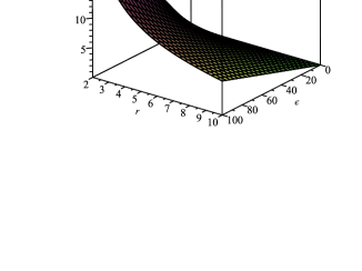
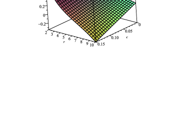
Figure 1: Variation of $T^{D}_{00}=\mu^{D}$ as function of $r$ and $\epsilon$

Figure 2: Variation of $T^{D}_{11}=P^{D}_{r}$ as function of $r$ and $\epsilon$

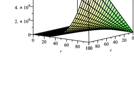
Figure 3: Variation of $T^{D}_{22}=P^{D}_{\perp}$ as function of $r$ and $\epsilon$

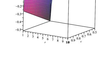
Figure 4: Variation of $\mu^{m}$ as function of $r$ and $\epsilon$

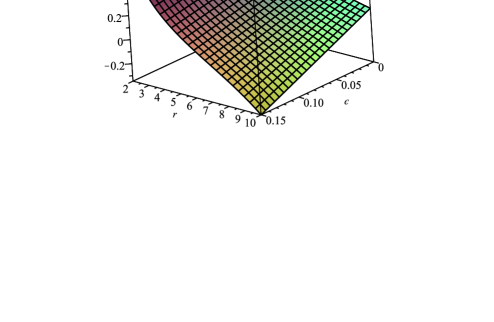
Figure 5: Variation of $P^{m}_{r}$ as function of $r$ and $\epsilon$

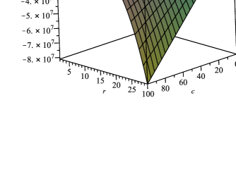
Figure 6: Variation of $P^{m}_{\perp}$ as function of $r$ and $\epsilon$

8 Conclusion

In this paper, we have studied cluster of stars in spherically symmetrical form where the fluid particles are a combination of baryonic (stars of clusters) and non-baryonic (DM) types matter. We have used the concept of high curvature gravity ($f(R)$ gravity) to include DM in the discussion. We have explored various simple modes of evolving cluster with the help of structure scalars in Starobinsky model, $f(R)=R+\varepsilon R^{2}$, to find the effects of non-baryonic matters on the evolution of stars cluster.

The structure scalars are used for exploring dynamics of self-gravitating structures. These factors refined the stellar evolution mechanism by reducing the system’s complexity. We have used the generalized definition of structure scalars in $f(R)$ gravity to propose the dynamics of refine (complex less) evolution of clusters. It has found that these scalars controls effects of tidal forces (Weyl tensor), effective anisotropic pressure and effective dissipative as well as inhomogeneous energy density factors. It has also been shown that the structure scalars suggested that structure of spherically symmetric cluster can be either isotropic or conformally flat and the two forces anisotropic stress and tidal force support each other.

Galactic observations indicated that the life and evolution of clusters depend on a considerable amount of DM. This shows that the DM can affect the evolving structure of clusters. Firstly, we have studied evolution with homogenous density and isotropic case. It is noticed that non-dissipative evolution shows density homogeneity if the anisotropic pressure of the fluid counteract with the tidal forces effects. The dissipative case depends upon dissipative factors due to baryonic matter as well as DM along with expansion and shear effects. The dissipating cluster having expansion and shear effects shows density inhomogeneity. For expansion and shear free situation, the dissipative evolution shows isotropic behavior with homogenous density.

We then have discussed homologous evolution for stars cluster in the presence of non-baryonic matter. For non-relativistic homologous evolution, it has found that if the cluster does not show shear as well as dissipative effects, then the velocity of evolving cluster is monitored by high curvature terms (DM terms) in the radial direction. So vanishes of higher curvature terms ($f(R)\sim R$) causes homologous evolution. Whereas in shear and non-dissipative case, this type of evolution take place if the DM terms canceled out the shear effects. It is noticed that, in GR, such type of evolution take place in shear-free and non-dissipative case but in higher curvature scenario the homologous evolution can take place in shear case as well.

The relativistic type of homologous evolution has also been explored. It is found that in either situations dissipative or non-dissipative DM terms play a important role in controlling homologous condition. Moreover, in contrast to GR results, it is concluded that the homologous evolution of cluster of star can be dissipative and shear-free or can be non-dissipative with shear effects.

We have explored condition for expanding cluster. It is concluded that expanding cluster depends upon shear effects along with dissipation due to matter and DM. The geodesic evolution also have investigated and it is obtained that the stars cluster moves with constant velocity. But around the center the fluid becomes homologous which shows geodesic and homologous imply each other.

Finally we explore behavior of Starobinsky model for a self-gravitating stellar $4U1820-30$ for values of parameter $\epsilon$ toward center. It has concluded that for large values of $\epsilon$ the density of DM becomes dominant as compare to matter density. The radial pressures remain dominant and increasing for both DM and baryonic matter. While the tangential pressures of both matter decreases to zero.

References

- [1] Planck collaboration, Ade, P.A.R. et al.: Planck 2013 Results. I. Overview of Products and Scientific Results, Astron. Astrophys. 571(2014)A1.
- [2] Buchdahl, H.A.: Mon. Not. Roy. Astron. Soc. 150(1070)1; Barrow, J.D. and Ottewill, A. C.: J. Phys. A: Math. Gen. 16(1983)2757; Nojiri, S. et al.: Phys. Rept. 692(2017)1.
- [3] Capozzilleo, S.: Int. Mod. Phys. D 11(2002)483; Nojiri, S. and Odintsov, S.D.: Phys. Rep. 505(2011)59; Capozziello, S. et al.: Phys. Rev. D 83(2011)064004.
- [4] Boehmer, G.C. et al.: Astropat. Phys. 29(2008)386; Capazziello, S. and De- Laurentis, M.F.: Ann. Phys. 524(2012)545. Cembranos, J. A. R. et al.: J. Cosmol. Astropart. Phys. 4(2012)021.
- [5] Starobinsky, A.A.: Phys. Lett. B 91(1980)99; Gottlber, S., Mller, V. and Satrobinsky, A.A.: Phys. Rev. D 43(1991)2510.
- [6] Cembrsnos,J.A.R.: Phys.Rev.Lett 102(2009)141301; J. Phys. Conf. Ser.315(2011)012004.
- [7] Baumgardt, H. and Makino, J.: Mon. Not. R. Astron. Soc. 340(2003)227; Kruijssen, J.M.D. et al.: Mon. Not. R. Astron. Soc. 414(2011)1364.
- [8] Herrera, L. et al.: Phys. Rev. D 79(2009)064025.
- [9] Herrera, L. Di Prisco, A. and Ibnez J.: Phys. Rev. D 84(2011) 064036.
- [10] L. Herrera, A. Di Prisco, and J. Ibnez.: Phys. Rev. D 84(2011)107501.
- [11] Herrera, L., Di Prisco, A. and Ospino J.: Gen. Relativ. Grav. 44(2012)2645; Herrera, L. et al.: Phys. Rev. D 89(2014)084034.
- [12] Herrera, L., Di Prisco, A. and Ospino J.: Phys. Rev. D 98(2018)104059); Eur. Phys. J. C 80(2020)631.
- [13] Sharif, M. and Manzoor, R.: Gen. Relativ. Gravit. 47(2015)98; Phys. Rev. D 91(2015)024018; Int. J. Mod. Phys. D 26(2017)1750057; Annals of Phys. 376(2017)1.
- [14] Yousaf, Z., Bhatti, M.Z. and Saleem, R.: Eur. Phys. J. Plus 134(2019)142; Yousaf, Z.: Eur. Phys. J. Plus 134(2019)245.
- [15] Praagman, A. and Hurley, J.: New Astronomy, 15(2010)1384.
- [16] Oort, J.H.: Astron. Inst. Neth. 6(1932)249; ibid 494(1960)45. Zwicky, W.H.: Phys. Acta. 6(1933)110.
- [17] Sharif, M. and Manzoor, R.: Mod. Phys. Lett. A 29(2014)1450192; As- trophys. Space Sci. 354(2014)497; Astrophys. Space Sci. 359(2015)17. Eur. Phys. Plus. 131(2016)64; Eur. Phys. J. C 76(2016)276; ibid. 330.
- [18] Jawad, A. et al.: Phys. Dark Univer. 21(2018)70; Rani, S. et al.: Eur. Phys. J. C 78(2016)1; Manzoor, R. et al.: Eur. Phys. J. C 79(2019)831; Manzoor, R., Adeel, M. and Saeed, M.: IJMPD 29(2020)2050036.
- [19] Herrera, L. et al.: Phys. Rev. D 69(2004)084026.
- [20] Hansen, C. and Kawaler, S.: Stellar Interiors: Physical Principles, Structure and Evolutions, (Springer Verlog, Berlin) (1994).
- [21] Jaffe, W.: MNRAS 202(1983)995.
- [22] Hernquist L.: Astro Physical J 356(1990)359.
- [23] Krori, K.D. and Barua, J.: J. Phys. A.: Math. Gen. 8(1975)508.
- [24] Bhar, Piyali.: Eur. Phys. J C 79(2019)138.
- [25] Zhang, W. et al.: Astro Physical J L500(1998)171.
- [26] Guver, T. et al.: Astro Physical J 719(2010)1807.