Partial recovery and weak consistency in the non-uniform hypergraph Stochastic Block Model

Abstract.

We consider the community detection problem in sparse random hypergraphs under the non-uniform hypergraph stochastic block model (HSBM), a general model of random networks with community structure and higher-order interactions. When the random hypergraph has bounded expected degrees, we provide a spectral algorithm that outputs a partition with at least a $\gamma$ fraction of the vertices classified correctly, where $\gamma\in(0.5,1)$ depends on the signal-to-noise ratio (SNR) of the model. When the SNR grows slowly as the number of vertices goes to infinity, our algorithm achieves weak consistency, which improves the previous results in [29] for non-uniform HSBMs.

Our spectral algorithm consists of three major steps: (1) Hyperedge selection: select hyperedges of certain sizes to provide the maximal signal-to-noise ratio for the induced sub-hypergraph; (2) Spectral partition: construct a regularized adjacency matrix and obtain an approximate partition based on singular vectors; (3) Correction and merging: incorporate the hyperedge information from adjacency tensors to upgrade the error rate guarantee. The theoretical analysis of our algorithm relies on the concentration and regularization of the adjacency matrix for sparse non-uniform random hypergraphs, which can be of independent interest.

1. Introduction

Clustering is one of the central problems in network analysis and machine learning [54, 60, 55]. Many clustering algorithms make use of graph models, which represent pairwise relationships among data. A well-studied probabilistic model is the stochastic block model (SBM), which was first introduced in [34] as a random graph model that generates community structure with given ground truth for clusters so that one can study algorithm accuracy. The past decades have brought many notable results in the analysis of different algorithms and fundamental limits for community detection in SBMs in different settings [19, 65, 32, 49]. A major breakthrough was the proof of phase transition behaviors of community detection algorithms in various connectivity regimes [47, 11, 50, 53, 52, 2, 5]. See the survey [1] for more references.

Hypergraphs can represent more complex relationships among data [10, 9], including recommendation systems [12, 44], computer vision [31, 66], and biological networks [48, 63], and they have been shown empirically to have advantages over graphs [72]. Besides community detection problems, sparse hypergraphs and their spectral theory have also found applications in data science [35, 73, 33], combinatorics [23, 26, 61], and statistical physics [13, 59].

With the motivation from a broad set of applications, many efforts have been made in recent years to study community detection on random hypergraphs. The hypergraph stochastic block model (HSBM), as a generalization of graph SBM, was first introduced and studied in [28]. In this model, we observe a random uniform hypergraph where each hyperedge appears independently with some given probability depending on the community structure of the vertices in the hyperedge.

Succinctly put, the HSBM recovery problem is to find the ground truth clusters either approximately or exactly, given a sample hypergraph and estimates of model parameters. We may ask the following questions about the quality of the solutions (see [1] for further details in the graph case).

1. Strong consistency (exact recovery): With high probability, find all clusters exactly (up to permutation).

2. Weak consistency (almost exact recovery): With high probability, find a partition of the vertex set such that at most $o(n)$ vertices are misclassified.

3. Partial recovery: Given a fixed $\gamma\in(0.5,1)$, with high probability, find a partition of the vertex set such that at least a fraction $\gamma$ of the vertices are clustered correctly.

4. Detection: With high probability, find a partition correlated with the true partition.

For exact recovery of uniform HSBMs, it was shown that the phase transition occurs in the regime of logarithmic expected degrees in [45, 16, 15] and the exact threshold was given in [38, 70, 27], by a generalization of techniques in [2, 4, 3]. Spectral methods were considered in [15, 6, 20, 70, 68], while semidefinite programming methods were analyzed in [38, 41]. Weak consistency for HSBMs was studied in [15, 16, 29, 30, 37]. For detection of the HSBM, the authors of [8] proposed a conjecture that the phase transition occurs in the regime of constant expected degrees, and the positive part of the conjecture for the binary and multi-block case were solved in [57] and [62] respectively. However, their results do not imply partial recovery: it only proves that above the Kesten-Stigum threshold, the algorithm can output a partition better than a random guess.

1.1. Non-uniform hypergraph stochastic block model

The non-uniform HSBM was first studied in [29], which removed the uniform hypergraph assumption in previous works, and it is a more realistic model to study higher-order interaction on networks [46, 66]. It can be seen as a superposition of several uniform HSBMs with different model parameters. We first define the uniform HSBM in our setting and extend it to non-uniform hypergraphs.

Definition 1.1 (Uniform HSBM).

Let $V=\{V_{1},\dots V_{k}\}$ be a partition of the set $[n]$ into $k$ blocks of size $\frac{n}{k}$ (assuming $n$ is divisible by $k$). For any set of $m$ distinct vertices $i_{1},\dots i_{m}$, a hyperedge $\{i_{1},\dots i_{m}\}$ is generated with probability $a_{m}/\binom{n}{m-1}$ if vertices $i_{1},\dots i_{m}$ are in the same block; otherwise with probability $b_{m}/\binom{n}{m-1}$. We denote this distribution on the set of $m$-uniform hypergraphs as

(1.1) $$H_{m}\sim\textnormal{HSBM}_{m}\left(\frac{n}{k},\frac{a_{m}}{\binom{n}{m-1}},\frac{b_{m}}{\binom{n}{m-1}}\right)\,,\quad 2\leq m\leq M\,.$$

Definition 1.2 (Non-uniform HSBM).

Let $H=(V,E)$ be a non-uniform random hypergraph, which can be considered as a collection of $m$-uniform hypergraphs, i.e., $H=\bigcup_{m=2}^{M}H_{m}$ with each $H_{m}$ from Equation 1.1.

Examples of $2$-uniform and $3$-uniform HSBM, and an example of non-uniform HSBM with $M=3$ and $k=3$ can be seen in Figure 1(a), Figure 1(b), Figure 1(c) respectively.

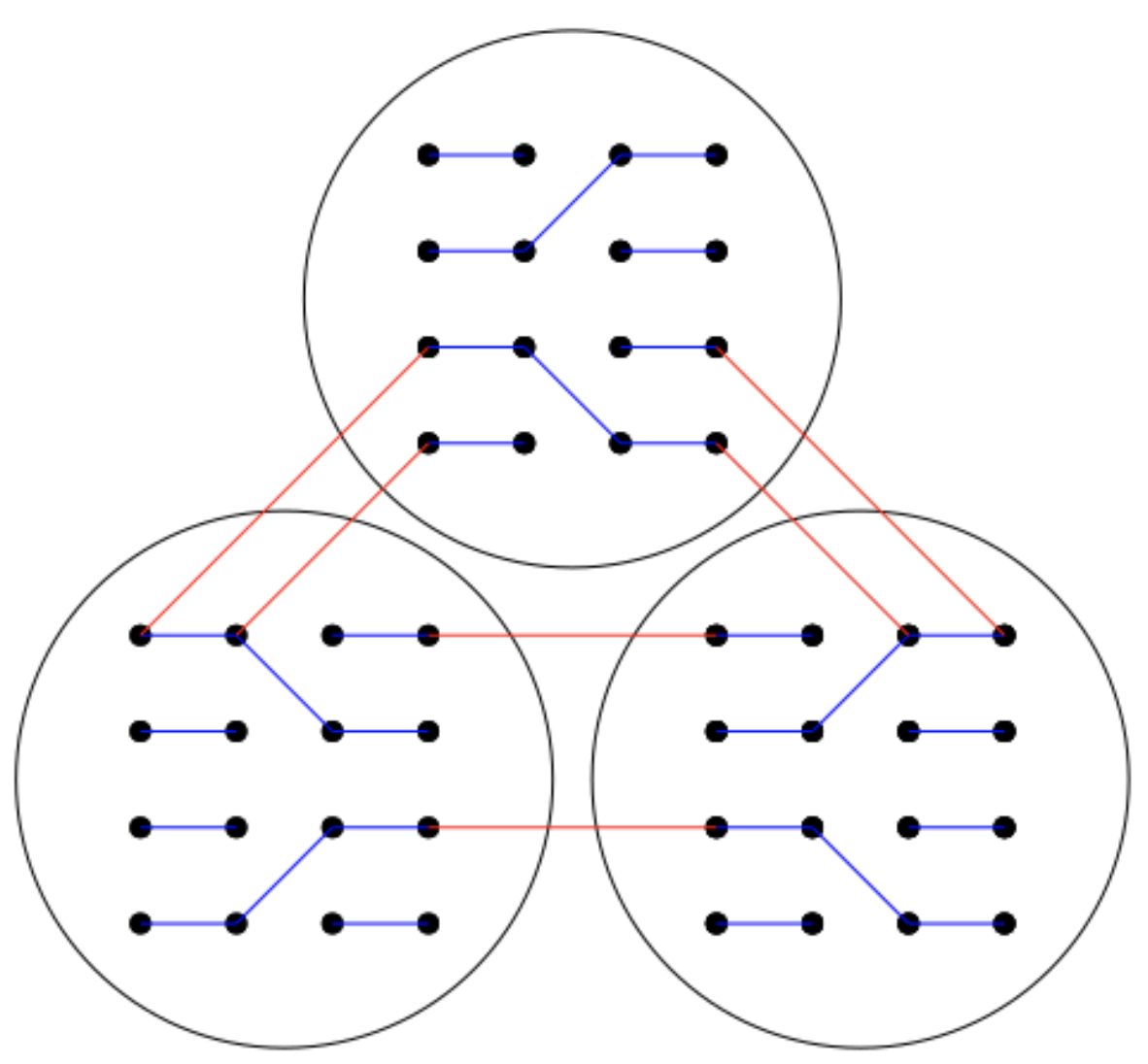
(a) 2-uniform HSBM

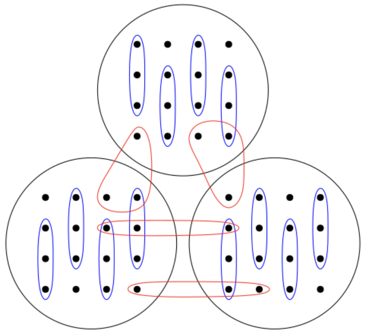
(b) 3-uniform HSBM

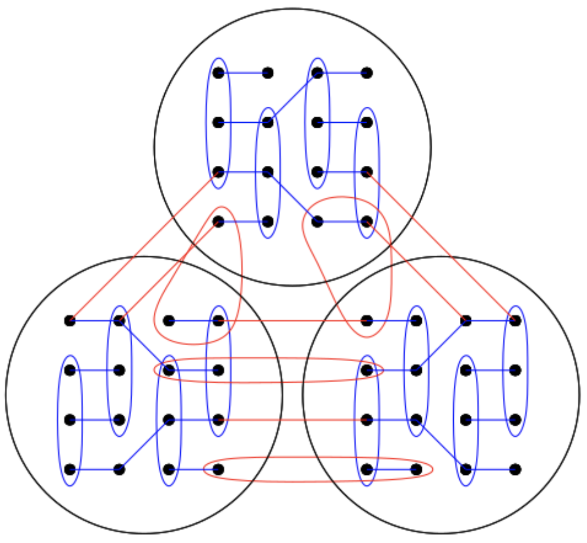
(c) Non-uniform HSBM

1.2. Main results

In this paper, we consider partial recovery and weak consistency in the non-uniform HSBM given in Definition 1.2. The accuracy of recovery is measured as follows.

Definition 1.3 ($\gamma$-correctness).

Suppose we have $k$ disjoint blocks $V_{1},\dots,V_{k}$. A collection of subsets $\widehat{V}_{1},\dots,\widehat{V}_{k}$ of $V$ is $\gamma$-correct if $|V_{i}\cap\widehat{V}_{i}|\geq\gamma|V_{i}|$ for all $i\in[k]$.

The following theorem provides an algorithm that outputs a $\gamma$-correct partition of a non-uniform HSBM with high probability when $k\geq 3$ is fixed.

Theorem 1.4 ($k\geq 3$).

Given any $\nu\in(0.5,1)$, assume $a_{m}\geq b_{m}$ are constants independent of $n$ for all $m\in\mathcal{M}$, where $\mathcal{M}\subset\{2,\dots,M\}$ is obtained from Algorithm 1 with $\mathcal{M}_{\max}$ denoting its maximum, and

$$d:=\sum_{m\in\mathcal{M}}(m-1)a_{m} \geq C,$$

(1.2) $$\sum_{m\in\mathcal{M}}(m-1)(a_{m}-b_{m}) \geq C_{\nu}\cdot k^{\mathcal{M}_{\max}-1}\sqrt{\log\Big{(}\frac{k}{1-\nu}\Big{)}d\,\,}$$

for some constants $C,C_{\nu}$. Then with probability $1-O(n^{-2})$, Algorithm 1 outputs a $\gamma$-correct partition with $\gamma=\max\{\nu,\,1-k\rho\}$ and $\rho:=\exp\left(-C_{\mathcal{M}}\cdot\mathrm{SNR}_{\mathcal{M}}\right)$ for sufficiently large $n$, where

(1.3) $$\mathrm{SNR}_{\mathcal{M}}:=\frac{\left[\sum_{m\in\mathcal{M}}(m-1)\left(\frac{a_{m}-b_{m}}{k^{m-1}}\right)\right]^{2}}{\sum_{m\in\mathcal{M}}(m-1)\left(\frac{a_{m}-b_{m}}{k^{m-1}}+b_{m}\right)}\,,\quad C_{\mathcal{M}}:=\frac{[\nu^{\mathcal{M}_{\max}-1}-(1-\nu)^{\mathcal{M}_{\max}-1}]^{2}}{(\mathcal{M}_{\max}-1)^{2}\cdot 2^{2\mathcal{M}_{\max}+3}}\,.$$

Remark 1.5.

Taking $M=2$, Theorem 1.4 can be reduced to [18, Lemma 9] for the graph case. The failure probability $O(n^{-2})$ can be decreased to $O(n^{-p})$ for any $p>0$, as long as one is willing to pay a price to make the graph denser (increasing $d$).

Our Algorithm 1 can be summarized in 3 steps:

1. Hyperedge selection: select hyperedges of certain sizes to provide the maximal signal-to-noise ratio (SNR) for the induced sub-hypergraph.

2. Spectral partition: construct a regularized adjacency matrix and obtain an approximate partition based on singular vectors (first approximation).

3. Correction and merging: incorporate the hyperedge information from adjacency tensors to upgrade the error rate guarantee (second, better approximation).

The algorithm requires the input of model parameters $a_{m},b_{m}$, which can be estimated by counting cycles in hypergraphs as shown in [50, 67]. Estimation of the number of blocks can be done by counting the outliers in the spectrum of the non-backtracking operator, e.g., as shown (for different regimes and different problems) in [58, 8, 39, 62]. However, this estimation method in non-uniform HSBM has not been rigorously justified.

Algorithm 1 Partition

1:The adjacency tensors $\boldsymbol{\mathcal{T}}_{m}$, $k$, $a_{m}$, $b_{m}$ for $m\in\{2,\cdots,M\}$.

2:The corrected sets $\widehat{V}_{1},\cdots,\widehat{V}_{k}$.

3:Run Algorithm 1 Pre-processing to obtain subset $\mathcal{M}$ which achieves the maximal $\mathrm{SNR}$.

4:Randomly color the hyperedges red or blue with equal probability.

5:Randomly partition $V$ into $2$ disjoint subsets $Y$ and $Z$ by assigning $+1$ or $-1$ to each vertex with equal probability.

6:Let ${\boldsymbol{\rm{B}}}$ denote the adjacency matrix of the bipartite hypergraph between $Y$ and $Z$ consisting only of the red hyperedges, with rows indexed by $Z$ and columns indexed by $Y$.

7:Run Algorithm 2 Spectral Partition on the red hypergraph and output $U_{1}^{\prime},\cdots,U_{k}^{\prime}$.
This step only uses the red hyperedges between vertices in $Y$ and $Z$ and outputs approximate clusters for $U_{i}:=V_{i}\cap Z$, with $i=1,\ldots,k$

8:Run Algorithm 3 Correction on the red hypergraph and output $\widehat{U}_{1},\cdots,\widehat{U}_{k}$.

9:Run Algorithm 4 Merging on the blue hypergraph and output $\widehat{V}_{1},\cdots,\widehat{V}_{k}$.
This step only uses the blue hyperedges between vertices in $Y$ and $Z$ and assigns the vertices in $Y$ to an appropriate approximate cluster.

We generalize the innovative graph algorithm in [18] to non-uniform hypergraphs with a more detailed analysis. In particular, the random partitioning step in Algorithm 2 was explained only in the case when the output is an equipartition; in general, the output sets $\widehat{V}_{1},\ldots,\widehat{V}_{k}$ are only approximately equal in size, and we give complete explanations for the general case.

A non-uniform HSBM can be seen as a collection of noisy observations for the same underlying community structure through several uniform HSBMs of different orders. A possible issue is that some uniform hypergraphs with small SNR might not be informative (if we observe an $m$-uniform hypergraph with parameters $a_{m}=b_{m}$, including hyperedge information from it ultimately increases the noise). To improve our error rate guarantees, we start by adding a pre-processing step for hyperedge selection according to SNR, and then apply the algorithm on the sub-hypergraph with maximal SNR.

When the number of blocks is $2$, we give a simpler algorithm (Algorithm 2) for partial recovery with a better error rate guarantee, as shown in the following Theorem 1.6. Algorithm 2 does not need the merging routine in Algorithm 1, since once we cluster one block, the other one is finished automatically.

Theorem 1.6 ($k=2$).

Given $\nu\in(0.5,1)$, assume $a_{m}\geq b_{m}$ are constants independent of $n$ for all $m\in\mathcal{M}$,

$$d:=\sum_{m\in\mathcal{M}}(m-1)a_{m} \geq C\,,$$

$$\sum_{m\in\mathcal{M}}(m-1)(a_{m}-b_{m}) \geq C_{\nu}\cdot 2^{\mathcal{M}_{\max}+2}\sqrt{d}\,,$$

for some constants $C,C_{\nu}$. Then with probability $1-O(n^{-2})$, Algorithm 2 outputs a $\gamma$-correct partition with $\gamma=\max\{\nu,\,1-2\rho\}$ and $\rho=2\exp(-C_{\mathcal{M}}\cdot\mathrm{SNR}_{\mathcal{M}})$ for sufficiently large $n$, where

(1.5) $$\mathrm{SNR}_{\mathcal{M}}:=\frac{\left[\sum_{m\in\mathcal{M}}(m-1)\left(\frac{a_{m}-b_{m}}{2^{m-1}}\right)\right]^{2}}{\sum_{m\in\mathcal{M}}(m-1)\left(\frac{a_{m}-b_{m}}{2^{m-1}}+b_{m}\right)}\,,\quad C_{\mathcal{M}}:=\frac{[(\nu)^{\mathcal{M}_{\max}-1}-(1-\nu)^{\mathcal{M}_{\max}-1}]^{2}}{8(\mathcal{M}_{\max}-1)^{2}}\,.$$

Algorithm 2 Binary Partition

1:The adjacency tensors $\boldsymbol{\mathcal{T}}^{(m)}$, $a_{m}$, $b_{m}$ for $m\in\{2,\cdots,M\}$.

2:The corrected sets $\widehat{V}_{1},\widehat{V}_{2}$. Ensure

3:Run Algorithm 1 Pre-processing to obtain subset $\mathcal{M}$ which achieves maximal $\mathrm{SNR}$.

4:Randomly color the hyperedges red or blue with equal probability.

5:Run Algorithm 5 Spectral Partition on the red hypergraph and output $V_{1}^{\prime},V_{2}^{\prime}$.

6:Run Algorithm 6 Correction on the blue hypergraph and output $\widehat{V}_{1},\widehat{V}_{2}$.

7:return The corrected sets $\widehat{V}_{1},\widehat{V}_{2}$.

Throughout the proofs for Theorem 1.4 and Theorem 1.6, we make only one assumption on the growth or finiteness of $d$ and $\mathrm{SNR}_{\mathcal{M}}$, and it happens in estimating the failure probability as noted in Remark 5.15. Consequently, the corollary below follows, which covers the case when $d$ and $\mathrm{SNR}_{\mathcal{M}}$ grow with $n$.

Corollary 1.7 (Weak consistency).

For fixed $M$ and $k$, if $\mathrm{SNR}_{\mathcal{M}}$ defined Equation 1.3 (resp. (1.5) ) goes to infinity as $n\to\infty$ and $\mathrm{SNR}_{\mathcal{M}}=o(\log n)$, then with probability $1-O(n^{-2})$, Algorithm 1 (resp. 2 ) outputs a partition with only $o(n)$ misclassified vertices.

The failure probability is of order $O(e^{-n\exp(-\mathrm{SNR}_{\mathcal{M}})})$, failing to go to zero if $\mathrm{SNR}_{\mathcal{M}}\gtrsim\log(n)$.

1.3. Comparison with existing results

Although many algorithms and theoretical results have been developed for hypergraph community detection, most of them are restricted to uniform hypergraphs, and few results are known for non-uniform ones. We will discuss the most relevant results.

In [37], the authors studied the degree-corrected HSBM with general connection probability parameters by using a tensor power iteration algorithm and Tucker decomposition. Their algorithm achieves weak consistency for uniform hypergraphs when the average degree is $\omega(\log^{2}n)$, which is the regime complementary to the regime we studied here. They discussed a way to generalize the algorithm to non-uniform hypergraphs, but the theoretical analysis remains open. The recent paper [71] analyzed non-uniform hypergraph community detection by using hypergraph embedding and optimization algorithms and obtained weak consistency when the expected degrees are of $\omega(\log n)$, again a complementary regime to ours. Results on spectral norm concentration of sparse random tensors were obtained in [22, 56, 35, 42, 73], but no provable tensor algorithm in the bounded expected degree is known. Testing for the community structure for non-uniform hypergraphs was studied in [67, 36], which is a problem different from community detection.

In our approach, we relied on knowing the tensors for each uniform hypergraph. However, in computations, we only ran the spectral algorithm on the adjacency matrix of the entire hypergraph, since the stability of tensor algorithms does not yet come with guarantees due to the lack of concentration, and for non-uniform hypergraphs, $M-1$ adjacency tensors would be needed. This approach presented the challenge that, unlike for graphs, the adjacency matrix of a random non-uniform hypergraph has dependent entries, and the concentration properties of such a random matrix were previously unknown. We were able to overcome this issue and prove concentration bounds from scratch, down to the bounded degree regime. Similar to [25, 40], we provided here a regularization analysis by removing rows in the adjacency matrix with large row sums (suggestive of large degree vertices) and proving a concentration result for the regularized matrix down to the bounded expected degree regime (see Theorem 3.3).

In terms of partial recovery for hypergraphs, our results are new, even in the uniform case. In [7, Theorem 1], for uniform hypergraphs, the authors showed detection (not partial recovery) is possible when the average degree is $\Omega(\frac{1}{n})$; in addition, the error rate is not exponential in the model parameters, but only polynomial. We mention here two more results for the graph case. In the arbitrarily slowly growing degrees regime, it was shown in [69, 24] that the error rate in Equation 1.3 is optimal up to a constant in the exponent. In the bounded expected degrees regime, the authors in [51, 17] provided algorithms that can asymptotically recover the optimal fraction of vertices, when the signal-to-noise ratio is large enough. It’s an open problem to extend their analysis to obtain a minimax error rate for hypergraphs.

In [29], the authors considered weak consistency in a non-uniform HSBM model with a spectral algorithm based on the hypergraph Laplacian matrix, and showed that weak consistency is achievable if the expected degree is of $\Omega(\log^{2}n)$ with high probability [28, Theorem 4.2]. Their algorithm can’t be applied to sparse regimes straightforwardly since the normalized Laplacian is not well-defined due to the existence of isolated vertices in the bounded degree case. In addition, our weak consistency results obtained here are valid as long as the expected degree is $\omega(1)$ and $o(\log n)$, which is the entire set of problems on which weak consistency is expected. By contrast, in [29], weak consistency is shown only when the expected degree is $\Omega(\log^{2}(n))$, which is a regime complementary to ours and where exact recovery should (in principle) be possible: for example, this is known to be an exact recovery regime in the uniform case [16, 38, 41, 70].

Finally, although our analysis does not provide a way to identify the exact threshold for the phase transition of detection in the non-uniform hypergraph, we conjecture that (similar to [8] in the uniform case) $\mathrm{SNR}_{\mathcal{M}}=1$ in Equation 2.5 is the exact threshold for detection.

1.4. Organization of the paper

In Section 2, we include the definitions of adjacency matrices of hypergraphs. The concentration results for the adjacency matrices are provided in Section 3. The algorithms for partial recovery are presented in Section 4. The proof for correctness of our algorithms for Theorem 1.4 and Corollary 1.7 are given in Section 5. The proof of Theorem 1.6 as well as the proofs of many auxiliary lemmas, and useful lemmas in the literature are provided in the supplemental materials.

2. Preliminaries

Definition 2.1 (Adjacency tensor).

Given an $m$-uniform hypergraph $H_{m}=([n],E_{m})$, we can associate to it an order-$m$ adjacency tensor $\boldsymbol{\mathcal{T}}^{(m)}$. For any $m$-hyperedge $e=\{i_{1},\dots,i_{m}\}$, let $\boldsymbol{\mathcal{T}}^{(m)}_{e}$ denote the corresponding entry $\boldsymbol{\mathcal{T}}_{[i_{1},\dots,i_{m}]}^{(m)}$, such that

(2.1) $$\boldsymbol{\mathcal{T}}_{e}^{(m)}:=\boldsymbol{\mathcal{T}}_{[i_{1},\dots,i_{m}]}^{(m)}=\mathbbm{1}_{\{e\in E_{m}\}}\,.$$

Definition 2.2 (Adjacency matrix).

For the non-uniform hypergraph $H$(Definition 1.2), let $\boldsymbol{\mathcal{T}}^{(m)}$ be the order-$m$ adjacency tensor corresponding to the underlying $m$-uniform hypergraph for each $m\in\{2,\dots,M\}$. The adjacency matrix ${\boldsymbol{\rm{A}}}:=[{\boldsymbol{\rm{A}}}_{ij}]_{n\times n}$ of the non-uniform hypergraph $H$ is defined by

(2.2) $${\boldsymbol{\rm{A}}}_{ij}=\mathbbm{1}_{\{i\neq j\}}\cdot\sum_{m=2}^{M}\,\,\sum_{\begin{subarray}{c}e\in E_{m}\\ \{i,j\}\subset e\end{subarray}}\boldsymbol{\mathcal{T}}^{(m)}_{e}\,.$$

We compute the expectation of ${\boldsymbol{\rm{A}}}$ first. In each $m$-uniform hypergraph $H_{m}$, two distinct vertices $i,j\in V$ with $i\neq j$ are picked arbitrarily, since our model does not allow for loops. Assume for a moment $\frac{n}{k}\in\mathbb{N}$, then the expected number of $m$-hyperedge containing $i$ and $j$ can be computed as follows.

• If $i$ and $j$ are from the same block, the $m$-hyperedge is sampled with probability $a_{m}/\binom{n}{m-1}$ when the other $m-2$ vertices are from the same block as $i$, $j$, otherwise with probability $b_{m}/\binom{n}{m-1}$. Then

  $$\alpha_{m}:=\mathbb{E}{\boldsymbol{\rm{A}}}_{ij}=\binom{\frac{n}{k}-2}{m-2}\frac{a_{m}}{\binom{n}{m-1}}+\left[\binom{n-2}{m-2}-\binom{\frac{n}{k}-2}{m-2}\right]\frac{b_{m}}{\binom{n}{m-1}}\,.$$

• If $i$ and $j$ are not from the same block, we sample the $m$-hyperedge with probability $b_{m}/\binom{n}{m-1}$, and

  $$\beta_{m}:=\mathbb{E}{\boldsymbol{\rm{A}}}_{ij}=\binom{n-2}{m-2}\frac{b_{m}}{\binom{n}{m-1}}\,.$$

By assumption $a_{m}\geq b_{m}$, then $\alpha_{m}\geq\beta_{m}$ for each $m\in\{2,\dots,M\}$. Summing over $m$, the expected adjacency matrix under the $k$-block non-uniform HSBM can be written as

(2.3) $$\mathbb{E}{\boldsymbol{\rm{A}}}=\begin{bmatrix}\alpha{\boldsymbol{\rm{J}}}_{\frac{n}{k}}&\beta{\boldsymbol{\rm{J}}}_{\frac{n}{k}}&\cdots&\beta{\boldsymbol{\rm{J}}}_{\frac{n}{k}}\\ \beta{\boldsymbol{\rm{J}}}_{\frac{n}{k}}&\alpha{\boldsymbol{\rm{J}}}_{\frac{n}{k}}&\cdots&\beta{\boldsymbol{\rm{J}}}_{\frac{n}{k}}\\ \vdots&\vdots&\ddots&\vdots\\ \beta{\boldsymbol{\rm{J}}}_{\frac{n}{k}}&\beta{\boldsymbol{\rm{J}}}_{\frac{n}{k}}&\cdots&\alpha{\boldsymbol{\rm{J}}}_{\frac{n}{k}}\end{bmatrix}-\alpha{\boldsymbol{\rm{I}}}_{n}\,,$$

where ${\boldsymbol{\rm{J}}}_{\frac{n}{k}}\in\mathbb{R}^{\frac{n}{k}\times\frac{n}{k}}$ denotes the all-one matrix and

(2.4) $$\alpha:=\sum_{m=2}^{M}\alpha_{m}\,,\quad\beta:=\sum_{m=2}^{M}\beta_{m}\,.$$

Lemma 2.3.

The eigenvalues of $\mathbb{E}{\boldsymbol{\rm{A}}}$ are given below:

$$\lambda_{1}(\mathbb{E}{\boldsymbol{\rm{A}}})= \,\frac{n}{k}(\alpha+(k-1)\beta)-\alpha\,,$$

$$\lambda_{i}(\mathbb{E}{\boldsymbol{\rm{A}}})= \,\frac{n}{k}(\alpha-\beta)-\alpha\,,\quad 2\leq i\leq k\,,$$

$$\lambda_{i}(\mathbb{E}{\boldsymbol{\rm{A}}})= \,-\alpha\,,~{}\quad\quad\quad k+1\leq i\leq n\,.$$

Lemma 2.3 can be verified via direct computation. Lemma 2.4 is used for approximately equi-partitions, meaning that eigenvalues of $\widetilde{\mathbb{E}{\boldsymbol{\rm{A}}}}$ can be approximated by eigenvalues $\mathbb{E}{\boldsymbol{\rm{A}}}$ when $n$ sufficiently large.

Lemma 2.4.

For any partition $(V_{1},\dots,V_{k})$ of $V$ where $n_{i}:=|V_{i}|$, consider the following matrix

$$\widetilde{\mathbb{E}{\boldsymbol{\rm{A}}}}=\begin{bmatrix}\alpha{\boldsymbol{\rm{J}}}_{n_{1}}&\beta{\boldsymbol{\rm{J}}}_{n_{1}\times n_{2}}&\cdots&\beta{\boldsymbol{\rm{J}}}_{n_{1}\times n_{k-1}}&\beta{\boldsymbol{\rm{J}}}_{n_{1}\times n_{k}}\\ \beta{\boldsymbol{\rm{J}}}_{n_{2}\times n_{1}}&\alpha{\boldsymbol{\rm{J}}}_{n_{2}}&\cdots&\beta{\boldsymbol{\rm{J}}}_{n_{2}\times n_{k-1}}&\beta{\boldsymbol{\rm{J}}}_{n_{2}\times n_{k}}\\ \vdots&\vdots&\ddots&\vdots&\vdots\\ \beta{\boldsymbol{\rm{J}}}_{n_{k-1}\times n_{1}}&\beta{\boldsymbol{\rm{J}}}_{n_{k-1}\times n_{2}}&\cdots&\alpha{\boldsymbol{\rm{J}}}_{n_{k-1}}&\beta{\boldsymbol{\rm{J}}}_{n_{k-1}\times n_{k}}\\ \beta{\boldsymbol{\rm{J}}}_{n_{k}\times n_{1}}&\beta{\boldsymbol{\rm{J}}}_{n_{k}\times n_{2}}&\cdots&\beta{\boldsymbol{\rm{J}}}_{n_{k}\times n_{k-1}}&\alpha{\boldsymbol{\rm{J}}}_{n_{k}}\end{bmatrix}-\alpha{\boldsymbol{\rm{I}}}_{n}\,.$$

Assume that $n_{i}=\frac{n}{k}+O(\sqrt{n}\log n)$ for all $i\in[k]$. Then, for all $1\leq i\leq k$,

$$\frac{|\lambda_{i}(\widetilde{\mathbb{E}{\boldsymbol{\rm{A}}}})-\lambda_{i}(\mathbb{E}{\boldsymbol{\rm{A}}})|}{|\lambda_{i}(\mathbb{E}{\boldsymbol{\rm{A}}})|}=O\Big{(}n^{-\frac{1}{4}}\log^{\frac{1}{2}}(n)\Big{)}\,.$$

Note that both $(\,\widetilde{\mathbb{E}{\boldsymbol{\rm{A}}}}+\alpha{\boldsymbol{\rm{I}}}_{n})$ and $(\,\mathbb{E}{\boldsymbol{\rm{A}}}+\alpha{\boldsymbol{\rm{I}}}_{n})$ are rank $k$ matrices, then $\lambda_{i}(\widetilde{\mathbb{E}{\boldsymbol{\rm{A}}}})=\lambda_{i}(\mathbb{E}{\boldsymbol{\rm{A}}})=-\alpha$ for all $(k+1)\leq i\leq n$.

Definition 2.5 (signal-to-noise ratio, $\mathrm{SNR}$).

We define the signal-to-noise ratio as

(2.5) $$\mathrm{SNR}:=\frac{\left[\sum_{m=2}^{M}(m-1)\left(\frac{a_{m}-b_{m}}{k^{m-1}}\right)\right]^{2}}{\sum_{m=2}^{M}(m-1)\left(\frac{a_{m}-b_{m}}{k^{m-1}}+b_{m}\right)}.$$

$\mathrm{SNR}$ is related to the following quantity

$$\,\frac{[\lambda_{2}(\mathbb{E}{\boldsymbol{\rm{A}}})]^{2}}{\lambda_{1}(\mathbb{E}{\boldsymbol{\rm{A}}})}=\frac{[(n-k)\alpha-n\beta]^{2}}{k[(n-k)\alpha+n(k-1)\beta]}=\frac{\left[\sum_{m=2}^{M}(m-1)\left(\frac{a_{m}-b_{m}}{k^{m-1}}\right)\right]^{2}}{\sum_{m=2}^{M}(m-1)\left(\frac{a_{m}-b_{m}}{k^{m-1}}+b_{m}\right)}(1+o(1)).$$

When $M=2$ and $k$ is fixed, Equation 2.5 is equal to $\frac{(a-b)^{2}}{k[a+(k-1)b]}$, which corresponds to the $\mathrm{SNR}$ for the undirected graph in [18], see also [1, Section 6].

3. Spectral norm concentration

The correctness of Algorithm 1 and Algorithm 2 relies on the concentration of the adjacency matrix of $H$. The following two concentration results for general random hypergraphs are included, which are independent of HSBM model. The proofs are deferred to Appendix A.

Theorem 3.1.

Let $H=\bigcup_{m=2}^{M}H_{m}$, where $H_{m}=([n],E_{m})$ is an Erdős-Rényi inhomogeneous hypergraph of order $m$ with $2\leq m\leq M$ with a probability tensor $\boldsymbol{\mathcal{T}}^{(m)}$ such that $\boldsymbol{\mathcal{T}}^{(m)}_{[i_{1},\dots,i_{m}]}=d_{[i_{1},\dots,i_{m}]}/\binom{n}{m-1}$ and $d_{m}=\max d_{[i_{1},\dots,i_{m}]}$. Suppose for some constant $c>0$,

(3.1) $$d:=\sum_{m=2}^{M}(m-1)\cdot d_{m}\geq c\log n\,.$$

Then for any $K>0$, there exists a constant $C=512M(M-1)(K+6)\left[2+(M-1)(1+K)/c\right]$ such that with probability at least $1-2n^{-K}-2e^{-n}$, the adjacency matrix ${\boldsymbol{\rm{A}}}$ of $H$ satisfies

(3.2) $$\|{\boldsymbol{\rm{A}}}-\mathbb{E}{\boldsymbol{\rm{A}}}\|\leq C\sqrt{d}\,.$$

Taking $M=2$, Equation 3.2 is the result for graph case obtained in [25, 43]. Result for uniform hypergraph is obtained in [41]. Note that $d$ is a fixed constant in our community detection problem, thus Equation 3.1 does not hold and Theorem 3.1 cannot be directly applied. However, we can still prove a concentration bound for a regularized version of ${\boldsymbol{\rm{A}}}$, following the same strategy of the proof for Theorem 3.1.

Definition 3.2 (Regularized matrix).

Given any $n\times n$ matrix ${\boldsymbol{\rm{A}}}$ and an index set ${\mathcal{I}}$, let ${\boldsymbol{\rm{A}}}_{{\mathcal{I}}}$ be the $n\times n$ matrix obtained from ${\boldsymbol{\rm{A}}}$ by zeroing out the rows and columns not indexed by ${\mathcal{I}}$. Namely,

(3.3) $$({\boldsymbol{\rm{A}}}_{{\mathcal{I}}})_{ij}=\mathbbm{1}_{\{i,j\in{\mathcal{I}}\}}\cdot{\boldsymbol{\rm{A}}}_{ij}\,.$$

Since every hyperedge of size $m$ containing $i$ is counted $(m-1)$ times in the $i$-th row sum of ${\boldsymbol{\rm{A}}}$, the $i$-th row sum of ${\boldsymbol{\rm{A}}}$ is given by

$$\textnormal{row}(i):=\sum_{j}{\boldsymbol{\rm{A}}}_{ij}:=\sum_{j}\mathbbm{1}_{\{i\neq j\}}\sum_{m=2}^{M}\,\,\sum_{\begin{subarray}{c}e\in E_{m}\\ \{i,j\}\subset e\end{subarray}}\boldsymbol{\mathcal{T}}^{(m)}_{e}=\sum_{m=2}^{M}\,(m-1)\sum_{e\in E_{m}:\,i\in e}\boldsymbol{\mathcal{T}}_{e}^{(m)}.$$

Theorem 3.3 is the concentration result for the regularized ${\boldsymbol{\rm{A}}}_{{\mathcal{I}}}$, by zeroing out rows and columns corresponding to vertices with high row sums.

Theorem 3.3.

Following all the notations in Theorem 3.1, for any constant $\tau>1$, define

$${\mathcal{I}}=\{i\in[n]:\textnormal{row}(i)\leq\tau d\}.$$

Let ${\boldsymbol{\rm{A}}}_{{\mathcal{I}}}$ be the regularized version of ${\boldsymbol{\rm{A}}}$, as in Definition 3.2. Then for any $K>0$, there exists a constant $C_{\tau}$ depending on $M,\tau,K$, such that $\|({\boldsymbol{\rm{A}}}-\mathbb{E}{\boldsymbol{\rm{A}}})_{{\mathcal{I}}}\|\leq C_{\tau}\sqrt{d}$ with probability at least $1-2(e/2)^{-n}-n^{-K}$.

4. Spectral algorithms

In this section, we present the algorithmic blocks that we use to construct our main partition algorithm (Algorithm 1): pre-processing (Algorithm 1), first attempt at partition (Algorithm 2), correction of blemishes via majority rule (Algorithm 3), and merging (Algorithm 4), together with their proofs of correctness. We start by giving the algorithms.

Algorithm 1 Pre-processing

1:For each subset $\mathcal{S}\subset\{2,\cdots,M\}$, let $H_{\mathcal{S}}=\bigcup_{m\in\mathcal{S}}H_{m}$ denote the restriction of the non-uniform hypergraph $H$ on $\mathcal{S}$. Compute $\mathrm{SNR}$ of $H_{\mathcal{S}}$, denoted by

$$\mathrm{SNR}_{\mathcal{S}}:=\frac{\left[\sum_{m\in\mathcal{S}}(m-1)\left(\frac{a_{m}-b_{m}}{k^{m-1}}\right)\right]^{2}}{\sum_{m\in\mathcal{S}}(m-1)\left(\frac{a_{m}-b_{m}}{k^{m-1}}+b_{m}\right)}\,.$$

2:Among all the $\mathcal{S}$, find the subset $\mathcal{M}$ such that

$$\mathcal{M}:=\arg\max_{\mathcal{S}\subset\{2,\cdots,M\}}\,\mathrm{SNR}_{\mathcal{S}}\,,$$

with $\mathcal{M}_{\max}$ denoting its maximal element.

3:return $\mathcal{M}$.

4.1. Three or more blocks ($k\geq 3$)

Algorithm 2 Spectral Partition

1:Randomly label vertices in $Y$ with $+1$ and $-1$ sign with equal probability, and partition $Y$ into $2$ disjoint subsets $Y_{1}$ and $Y_{2}$.

2:Let ${\boldsymbol{\rm{B}}}_{1}$ (resp. ${\boldsymbol{\rm{B}}}_{2}$) denote the adjacency matrices with all vertices in $Z\cup Y_{1}$, with rows indexed by $Z$ and columns indexed by $Y_{1}$ (resp. $Y_{2}$). Pad ${\boldsymbol{\rm{B}}}_{1}$, ${\boldsymbol{\rm{B}}}_{2}$ with zeros to obtain the $n\times n$ matrices ${\boldsymbol{\rm{A}}}_{1}$ and ${\boldsymbol{\rm{A}}}_{2}$.

3:Let $d:=\sum_{m\in\mathcal{M}}(m-1)a_{m}$. Zero out all the rows and columns of ${\boldsymbol{\rm{A}}}_{1}$ corresponding to vertices whose row sum is bigger than $20\mathcal{M}_{\max}d$, to obtain the matrix $({\boldsymbol{\rm{A}}}_{1})_{{\mathcal{I}}_{1}}$.

4:Find the space ${\boldsymbol{\rm{U}}}$, spanned by the first $k$ left singular vectors of $({\boldsymbol{\rm{A}}}_{1})_{{\mathcal{I}}_{1}}$.

5:Randomly sample $s=2k\log^{2}n$ vertices from $Y_{2}$ without replacement. Denote the corresponding columns in ${\boldsymbol{\rm{A}}}_{2}$ by ${\boldsymbol{a}}_{i_{1}},\dots,{\boldsymbol{a}}_{i_{s}}$. For each $i\in\{i_{1},\cdots,i_{s}\}$, project ${\boldsymbol{a}}_{i}-\overline{{\boldsymbol{a}}}$ onto ${\boldsymbol{\rm{U}}}$, where the elements in vector $\overline{{\boldsymbol{a}}}\in\mathbb{R}^{n}$ is defined by $\overline{{\boldsymbol{a}}}(j)=\mathbbm{1}_{j\in Z}\cdot(\overline{\alpha}+\overline{\beta})/2$, with $\overline{\alpha}$, $\overline{\beta}$ defined in Equation 5.6.

6:For each projected vector $P_{{\boldsymbol{\rm{U}}}}({\boldsymbol{a}}_{i}-\overline{{\boldsymbol{a}}})$, identify the top $n/(2k)$ coordinates in value as a set $U_{i}$. Discard half of the $s$ sets $U_{i}$, those with the lowest blue hyperedge density in them.

7:Sort the remaining sets according to blue hyperedge density and identify first $k$ distinct subsets $U^{\prime}_{1},\cdots,U^{\prime}_{k}$ such that $|U^{\prime}_{i}\cap U^{\prime}_{j}|<\lceil\frac{(1-\nu)n}{k}\rceil$ if $i\neq j$. return $U_{1}^{\prime},\cdots,U_{k}^{\prime}$.

Algorithm 3 Correction

1:For every $u\in Z$, if $i\in\{1,2,\cdots,k\}$ is such that $u$ has more neighbors in $U_{i}^{\prime}$ than in any other $U_{j}^{\prime}$, for $j\neq i$, then add $u$ to $\widehat{U}_{i}$. Break ties arbitrarily. return $\widehat{U}_{1},\cdots,\widehat{U}_{k}$.

Algorithm 4 Merging

1:For all $u\in Y$, add $u$ to $\widehat{U_{i}}$ if the number of hyperedges, which contains $u$ with the remaining vertices located in vertex set $\widehat{U}_{i}$, is at least $\mu_{\rm{M}}$. Label the conflicts arbitrarily.

2:return the label classes as the clusters $\widehat{V}_{1},\cdots,\widehat{V}_{k}$.

The proof of Theorem 1.4 is structured as follows.

Lemma 4.1.

Under the assumptions of Theorem 1.4, Algorithm 2 outputs a $\nu$-correct partition $U_{1}^{\prime},\cdots,U_{k}^{\prime}$ of $Z=(Z\cap V_{1})\cup\cdots\cup(Z\cap V_{k})$ with probability at least $1-O(n^{-2})$.

Lemma 4.2.

Under the assumptions of Theorem 1.4, for any $\nu$-correct partition $U_{1}^{\prime},\cdots,U_{k}^{\prime}$ of $Z=(Z\cap V_{1})\cup\cdots\cup(Z\cap V_{k})$ and the red hypergraph over $Z$, Algorithm 3 computes a $\gamma_{\rm{C}}$-correct partition $\widehat{U}_{1},\cdots,\widehat{U}_{k}$ with probability $1-O(e^{-n\rho})$, while $\gamma_{\rm{C}}=\max\{\nu,\,1-k\rho\}$ with $\rho:=k\exp\left(-C_{\mathcal{M}}\cdot\mathrm{SNR}_{\mathcal{M}}\right)$ where $\mathcal{M}$ is obtained from Algorithm 1, and $\mathrm{SNR}_{\mathcal{M}}$ and $C_{\mathcal{M}}$ are defined in Equation 1.3.

Lemma 4.3.

Given any $\nu$-correct partition $\widehat{U}_{1},\cdots,\widehat{U}_{k}$ of $Z=(Z\cap V_{1})\cup\cdots\cup(Z\cap V_{k})$ and the blue hypergraph between $Y$ and $Z$, with probability $1-O(e^{-n\rho})$, Algorithm 4 outputs a $\gamma$-correct partition $\widehat{V}_{1},\cdots,\widehat{V}_{k}$ of $V_{1}\cup V_{2}\cup\cdots\cup V_{k}$, while $\gamma=\max\{\nu,\,1-k\rho\}$.

4.2. The binary case ($k=2$)

The spectral partition step is given in Algorithm 5, and the correction step is given in Algorithm 6.

Algorithm 5 Spectral Partition

1:Zero out all the rows and the columns of ${\boldsymbol{\rm{A}}}$ corresponding to vertices with row sums greater than $20\mathcal{M}_{\max}d$, to obtain the regularized matrix ${\boldsymbol{\rm{A}}}_{{\mathcal{I}}}$.

2:Find the subspace ${\boldsymbol{\rm{U}}}$, which is spanned by the eigenvectors corresponding to the largest two eigenvalues of ${\boldsymbol{\rm{A}}}_{{\mathcal{I}}}$.

3:Compute $P_{{\boldsymbol{\rm{U}}}}\mathbf{1}_{n}$, the projection of all-ones vector onto ${\boldsymbol{\rm{U}}}$.

4:Let ${\boldsymbol{v}}$ be the unit vector in ${\boldsymbol{\rm{U}}}$ perpendicular to $P_{{\boldsymbol{\rm{U}}}}\mathbf{1}_{n}$.

5:Sort the vertices according to their values in ${\boldsymbol{v}}$. Let $V_{1}^{\prime}\subset V$ be the corresponding top $n/2$ vertices, and $V_{2}^{\prime}\subset V$ be the remaining $n/2$ vertices.

6:return $V_{1}^{\prime}$, $V_{2}^{\prime}$.

Lemma 4.4.

Under the conditions of Theorem 1.6, the Algorithm 5 outputs a $\nu$-correct partition $V_{1}^{\prime},V_{2}^{\prime}$ of $V=V_{1}\cup V_{2}$ with probability at least $1-O(n^{-2})$.

Algorithm 6 Correction

1:For any $v\in V_{1}^{\prime}$, label $v$ “bad” if the number of blue neighbors of $v$ in $V_{2}^{\prime}$ is at least $\frac{a+b}{4}$ and “good” otherwise.

2:Do the same for $v\in V_{2}^{\prime}$.

3:If $v\in V_{i}^{\prime}$ is good, assign it to $\widehat{V}_{i}$, otherwise $\widehat{V}_{3-i}$.

4:return $\widehat{V}_{1}$, $\widehat{V}_{2}$.

Lemma 4.5.

Given any $\nu$-correct partition $V_{1}^{\prime},V_{2}^{\prime}$ of $V=V_{1}\cup V_{2}$, with probability at least $1-O(e^{-n\rho})$, the Algorithm 6 computes a $\gamma$-correct partition $\widehat{V}_{1},\widehat{V}_{2}$ with $\gamma=\{\nu,\,1-2\rho\}$ and $\rho=2\exp(-C_{\mathcal{M}}\cdot\mathrm{SNR}_{\mathcal{M}})$, where $\mathrm{SNR}_{\mathcal{M}}$ and $C_{\mathcal{M}}$ are defined in Equation 1.5.

5. Algorithm’s correctness

In this section, we will show the correctness of Algorithm 1. We first introduce some definitions.

Vertex set splitting and adjacency matrix

In Algorithm 1, we first randomly partition the vertex set $V$ into two disjoint subsets $Z$ and $Y$ by assigning $+1$ and $-1$ to each vertex independently with equal probability. Let ${\boldsymbol{\rm{B}}}\in\mathbb{R}^{|Z|\times|Y|}$ denote the submatrix of ${\boldsymbol{\rm{A}}}$, while ${\boldsymbol{\rm{A}}}$ was defined in Equation 2.2, where rows and columns of ${\boldsymbol{\rm{B}}}$ correspond to vertices in $Z$ and $Y$ respectively. Let $n_{i}$ denote the number of vertices in $Z\cap V_{i}$, where $V_{i}$ denotes the true partition with $|V_{i}|=\frac{n}{k}$ for all $i\in[k]$, then $n_{i}$ can be written as a sum of independent Bernoulli random variables, i.e.,

(5.1) $$n_{i}=|Z\cap V_{i}|=\sum_{v\in V_{i}}\mathbbm{1}_{\{v\in Z\}}\,,$$

and $|Y\cap V_{i}|=|V_{i}|-|Z\cap V_{i}|=\frac{n}{k}-n_{i}$ for each $i\in[k]$.

Definition 5.1.

The splitting $V=Z\cup Y$ is perfect if $|Z\cap V_{i}|=|Y\cap V_{i}|=n/(2k)$ for all $i\in[k]$. And the splitting $Y=Y_{1}\cup Y_{2}$ is perfect if $|Y_{1}\cap V_{i}|=|Y_{2}\cap V_{i}|=n/(4k)$ for all $i\in[k]$.

However, the splitting will actually be imperfect in most cases, since the size of $Z$ and $Y$ would not be exactly the same under the independence assumption. The random matrix ${\boldsymbol{\rm{B}}}$ is parameterized by $\{\boldsymbol{\mathcal{T}}^{(m)}\}_{m\in\mathcal{M}}$ and $\{n_{i}\}_{i=1}^{k}$. If we take expectation over $\{\boldsymbol{\mathcal{T}}^{(m)}\}_{m\in\mathcal{M}}$ given the block size information $\{n_{i}\}_{i=1}^{k}$, then it gives rise to the expectation of the imperfect splitting, denoted by $\widetilde{{\boldsymbol{\rm{B}}}}$,

$$\widetilde{{\boldsymbol{\rm{B}}}}:=\begin{bmatrix}\alpha{\boldsymbol{\rm{J}}}_{n_{1}\times(\frac{n}{k}-n_{1})}&\beta{\boldsymbol{\rm{J}}}_{n_{1}\times(\frac{n}{k}-n_{2})}&\dots&\beta{\boldsymbol{\rm{J}}}_{n_{1}\times(\frac{n}{k}-n_{k})}\\ \beta{\boldsymbol{\rm{J}}}_{n_{2}\times(\frac{n}{k}-n_{1})}&\alpha{\boldsymbol{\rm{J}}}_{n_{2}\times(\frac{n}{k}-n_{2})}&\dots&\beta{\boldsymbol{\rm{J}}}_{n_{2}\times(\frac{n}{k}-n_{k})}\\ \vdots&\vdots&\ddots&\vdots\\ \beta{\boldsymbol{\rm{J}}}_{n_{k}\times(\frac{n}{k}-n_{1})}&\beta{\boldsymbol{\rm{J}}}_{n_{k}\times(\frac{n}{k}-n_{2})}&\dots&\alpha{\boldsymbol{\rm{J}}}_{n_{k}\times(\frac{n}{k}-n_{k})}\end{bmatrix}\,,$$

where $\alpha$, $\beta$ are defined in Equation 2.4. In the perfect splitting case, the dimension of each block is $n/(2k)\times n/(2k)$ since $\mathbb{E}n_{i}=n/(2k)$ for all $i\in[k]$, and the expectation matrix $\overline{{\boldsymbol{\rm{B}}}}$ can be written as

$$\overline{{\boldsymbol{\rm{B}}}}:=\begin{bmatrix}\alpha{\boldsymbol{\rm{J}}}_{\frac{n}{2k}}&\beta{\boldsymbol{\rm{J}}}_{\frac{n}{2k}}&\dots&\beta{\boldsymbol{\rm{J}}}_{\frac{n}{2k}}\\ \beta{\boldsymbol{\rm{J}}}_{\frac{n}{2k}}&\alpha{\boldsymbol{\rm{J}}}_{\frac{n}{2k}}&\dots&\beta{\boldsymbol{\rm{J}}}_{\frac{n}{2k}}\\ \vdots&\vdots&\ddots&\vdots\\ \beta{\boldsymbol{\rm{J}}}_{\frac{n}{2k}}&\beta{\boldsymbol{\rm{J}}}_{\frac{n}{2k}}&\dots&\alpha{\boldsymbol{\rm{J}}}_{\frac{n}{2k}}\end{bmatrix}\,.$$

In Algorithm 2, $Y_{1}$ is a random subset of $Y$ obtained by selecting each element with probability $1/2$ independently, and $Y_{2}=Y\setminus Y_{1}$. Let $n^{\prime}_{i}$ denote the number of vertices in $Y_{1}\cap V_{i}$, then $n^{\prime}_{i}$ can be written as a sum of independent Bernoulli random variables,

(5.2) $$n^{\prime}_{i}=|Y_{1}\cap V_{i}|=\sum_{v\in V_{i}}\mathbf{1}_{\{v\in Y_{1}\}}\,,$$

and $|Y_{2}\cap V_{i}|=|V_{i}|-|Z\cap V_{i}|-|Y_{1}\cap V_{i}|=n/k-n_{i}-n^{\prime}_{i}$ for all $i\in[k]$.

Induced sub-hypergraph

Definition 5.2 (Induced Sub-hypergraph).

Let $H=(V,E)$ be a non-uniform random hypergraph and $S\subset V$ be any subset of the vertices of $H$. Then the induced sub-hypergraph $H[S]$ is the hypergraph whose vertex set is $S$ and whose hyperedge set $E[S]$ consists of all of the edges in $E$ that have all endpoints located in $S$.

Let $H[Y_{1}\cup Z]$(resp. $H[Y_{2}\cup Z]$) denote the induced sub-hypergraph on vertex set $Y_{1}\cup Z$ (resp. $Y_{2}\cup Z$), and ${\boldsymbol{\rm{B}}}_{1}\in\mathbb{R}^{|Z|\times|Y_{1}|}$ (resp. ${\boldsymbol{\rm{B}}}_{2}\in\mathbb{R}^{|Z|\times|Y_{2}|}$) denote the adjacency matrices corresponding to the sub-hypergraphs, where rows and columns of ${\boldsymbol{\rm{B}}}_{1}$ (resp. ${\boldsymbol{\rm{B}}}_{2}$) are corresponding to elements in $Z$ and $Y_{1}$ (resp., $Z$ and $Y_{2}$). Therefore, ${\boldsymbol{\rm{B}}}_{1}$ and ${\boldsymbol{\rm{B}}}_{2}$ are parameterized by $\{\boldsymbol{\mathcal{T}}^{(m)}\}_{m\in\mathcal{M}}$, $\{n_{i}\}_{i=1}^{k}$ and $\{n^{\prime}_{i}\}_{i=1}^{k}$, and the entries in ${\boldsymbol{\rm{B}}}_{1}$ are independent of the entries in ${\boldsymbol{\rm{B}}}_{2}$, due to the independence of hyperedges. If we take expectation over $\{\boldsymbol{\mathcal{T}}^{(m)}\}_{m\in\mathcal{M}}$ conditioning on $\{n_{i}\}_{i=1}^{k}$ and $\{n^{\prime}_{i}\}_{i=1}^{k}$, then it gives rise to the expectation of the imperfect splitting, denoted by $\widetilde{{\boldsymbol{\rm{B}}}}_{1}$,

(5.3) $$\widetilde{{\boldsymbol{\rm{B}}}}_{1}:=\begin{bmatrix}\widetilde{\alpha}_{11}{\boldsymbol{\rm{J}}}_{n_{1}\times n^{\prime}_{1}}&\dots&\widetilde{\beta}_{1k}{\boldsymbol{\rm{J}}}_{n_{1}\times n^{\prime}_{k}}\\ \vdots&\ddots&\vdots\\ \widetilde{\beta}_{k1}{\boldsymbol{\rm{J}}}_{n_{k}\times n^{\prime}_{1}}&\dots&\widetilde{\alpha}_{kk}{\boldsymbol{\rm{J}}}_{n_{k}\times n^{\prime}_{k}}\end{bmatrix}\,,$$

where

(5.4a) $$\widetilde{\alpha}_{ii}:= \,\sum_{m\in\mathcal{M}}\left\{\binom{n_{i}+n_{i}^{\prime}-2}{m-2}\frac{a_{m}-b_{m}}{\binom{n}{m-1}}+\binom{\sum_{l=1}^{k}(n_{l}+n_{l}^{\prime})-2}{m-2}\frac{b_{m}}{\binom{n}{m-1}}\right\}\,,$$

(5.4b) $$\widetilde{\beta}_{ij}:= \,\sum_{m\in\mathcal{M}}\binom{\sum_{l=1}^{k}(n_{l}+n_{l}^{\prime})-2}{m-2}\frac{b_{m}}{\binom{n}{m-1}}\,,\quad i\neq j,\,i,j\in[k]\,.$$

The expectation of the perfect splitting, denoted by $\overline{{\boldsymbol{\rm{B}}}}_{1}$, can be written as

(5.5) $$\overline{{\boldsymbol{\rm{B}}}}_{1}:=\begin{bmatrix}\overline{\alpha}{\boldsymbol{\rm{J}}}_{\frac{n}{2k}\times\frac{n}{4k}}&\overline{\beta}{\boldsymbol{\rm{J}}}_{\frac{n}{2k}\times\frac{n}{4k}}&\dots&\overline{\beta}{\boldsymbol{\rm{J}}}_{\frac{n}{2k}\times\frac{n}{4k}}\\ \overline{\beta}{\boldsymbol{\rm{J}}}_{\frac{n}{2k}\times\frac{n}{4k}}&\overline{\alpha}{\boldsymbol{\rm{J}}}_{\frac{n}{2k}\times\frac{n}{4k}}&\dots&\overline{\beta}{\boldsymbol{\rm{J}}}_{\frac{n}{2k}\times\frac{n}{4k}}\\ \vdots&\vdots&\ddots&\vdots\\ \overline{\beta}{\boldsymbol{\rm{J}}}_{\frac{n}{2k}\times\frac{n}{4k}}&\overline{\beta}{\boldsymbol{\rm{J}}}_{\frac{n}{2k}\times\frac{n}{4k}}&\dots&\overline{\alpha}{\boldsymbol{\rm{J}}}_{\frac{n}{2k}\times\frac{n}{4k}}\end{bmatrix}\,,$$

where

(5.6) $$\overline{\alpha}:=\sum_{m\in\mathcal{M}}\left\{\binom{\frac{3n}{4k}-2}{m-2}\frac{a_{m}-b_{m}}{\binom{n}{m-1}}+\binom{\frac{3n}{4}-2}{m-2}\frac{b_{m}}{\binom{n}{m-1}}\right\}\,,\quad\overline{\beta}:=\sum_{m\in\mathcal{M}}\binom{\frac{3n}{4}-2}{m-2}\frac{b_{m}}{\binom{n}{m-1}}\,.$$

The matrices $\widetilde{{\boldsymbol{\rm{B}}}}_{2},\overline{{\boldsymbol{\rm{B}}}}_{2}$ can be defined similarly, since dimensions of $|Y_{2}\cap V_{i}|$ are also determined by $n_{i}$ and $n^{\prime}_{i}$. Obviously, $\overline{{\boldsymbol{\rm{B}}}}_{2}=\overline{{\boldsymbol{\rm{B}}}}_{1}$ since $\mathbb{E}n^{\prime}_{i}=\mathbb{E}(n/k-n_{i}-n_{i}^{\prime})=n/(4k)$ for all $i\in[k]$.

Fixing Dimensions

The dimensions of $\widetilde{{\boldsymbol{\rm{B}}}}_{1}$ and $\widetilde{{\boldsymbol{\rm{B}}}}_{2}$, as well as blocks they consist of, are not deterministic—since $n_{i}$ and $n^{\prime}_{i}$, defined in Equation 5.1 and Equation 5.2 respectively, are sums of independent random variables. As such we cannot directly compare them. In order to overcome this difficulty, we embed ${\boldsymbol{\rm{B}}}_{1}$ and ${\boldsymbol{\rm{B}}}_{2}$ into the following $n\times n$ matrices:

(5.7) $${\boldsymbol{\rm{A}}}_{1}:=\begin{bmatrix}\mathbf{0}_{|Z|\times|Z|}&{\boldsymbol{\rm{B}}}_{1}&\mathbf{0}_{|Z|\times|Y_{2}|}\\ \mathbf{0}_{|Y|\times|Z|}&\mathbf{0}_{|Y|\times|Y_{1}|}&\mathbf{0}_{|Y|\times|Y_{2}|}\end{bmatrix}\,,\quad{\boldsymbol{\rm{A}}}_{2}:=\begin{bmatrix}\mathbf{0}_{|Z|\times|Z|}&\mathbf{0}_{|Z|\times|Y_{1}|}&{\boldsymbol{\rm{B}}}_{2}\\ \mathbf{0}_{|Y|\times|Z|}&\mathbf{0}_{|Y|\times|Y_{1}|}&\mathbf{0}_{|Y|\times|Y_{2}|}\end{bmatrix}\,.$$

Note that ${\boldsymbol{\rm{A}}}_{1}$ and ${\boldsymbol{\rm{A}}}_{2}$ have the same size. Also by definition, the entries in ${\boldsymbol{\rm{A}}}_{1}$ are independent of the entries in ${\boldsymbol{\rm{A}}}_{2}$. If we take expectation over $\{\boldsymbol{\mathcal{T}}^{(m)}\}_{m\in\mathcal{M}}$ conditioning on $\{n_{i}\}_{i=1}^{k}$ and $\{n^{\prime}_{i}\}_{i=1}^{k}$, then we obtain the expectation matrices of the imperfect splitting, denoted by $\widetilde{{\boldsymbol{\rm{A}}}}_{1}$(resp. $\widetilde{{\boldsymbol{\rm{A}}}}_{2}$), written as

(5.8) $$\widetilde{{\boldsymbol{\rm{A}}}}_{1}:=\begin{bmatrix}\mathbf{0}_{|Z|\times|Z|}&\widetilde{{\boldsymbol{\rm{B}}}}_{1}&\mathbf{0}_{|Z|\times|Y_{2}|}\\ \mathbf{0}_{|Y|\times|Z|}&\mathbf{0}_{|Y|\times|Y_{1}|}&\mathbf{0}_{|Y|\times|Y_{2}|}\end{bmatrix}\,,\quad\widetilde{{\boldsymbol{\rm{A}}}}_{2}:=\begin{bmatrix}\mathbf{0}_{|Z|\times|Z|}&\mathbf{0}_{|Z|\times|Y_{1}|}&\widetilde{{\boldsymbol{\rm{B}}}}_{2}\\ \mathbf{0}_{|Y|\times|Z|}&\mathbf{0}_{|Y|\times|Y_{1}|}&\mathbf{0}_{|Y|\times|Y_{2}|}\end{bmatrix}\,.$$

The expectation matrix of the perfect splitting, denoted by $\overline{{\boldsymbol{\rm{A}}}}_{1}$(resp. $\overline{{\boldsymbol{\rm{A}}}}_{2}$), can be written as

(5.9) $$\overline{{\boldsymbol{\rm{A}}}}_{1}:=\begin{bmatrix}\mathbf{0}_{\frac{n}{2}\times\frac{n}{2}}&\overline{{\boldsymbol{\rm{B}}}}_{1}&\mathbf{0}_{\frac{n}{2}\times\frac{n}{4}}\\ \mathbf{0}_{\frac{n}{2}\times\frac{n}{2}}&\mathbf{0}_{\frac{n}{2}\times\frac{n}{4}}&\mathbf{0}_{\frac{n}{2}\times\frac{n}{4}}\end{bmatrix}\,,\quad\overline{{\boldsymbol{\rm{A}}}}_{2}:=\begin{bmatrix}\mathbf{0}_{\frac{n}{2}\times\frac{n}{2}}&\mathbf{0}_{\frac{n}{2}\times\frac{n}{4}}&\overline{{\boldsymbol{\rm{B}}}}_{2}\\ \mathbf{0}_{\frac{n}{2}\times\frac{n}{2}}&\mathbf{0}_{\frac{n}{2}\times\frac{n}{4}}&\mathbf{0}_{\frac{n}{2}\times\frac{n}{4}}\end{bmatrix}\,.$$

Obviously, $\widetilde{{\boldsymbol{\rm{A}}}}_{i}$ and $\widetilde{{\boldsymbol{\rm{B}}}}_{i}$(resp. $\overline{{\boldsymbol{\rm{A}}}}_{i}$ and $\overline{{\boldsymbol{\rm{B}}}}_{i}$) have the same non-zero singular values for $i=1,2$. In the remaining of this section, we will deal with $\widetilde{{\boldsymbol{\rm{A}}}}_{i}$ and $\overline{{\boldsymbol{\rm{A}}}}_{i}$ instead of $\widetilde{{\boldsymbol{\rm{B}}}}_{i}$ and $\overline{{\boldsymbol{\rm{B}}}}_{i}$ for $i=1,2$.

5.1. Spectral Partition: Proof of Lemma 4.1

5.1.1. Proof Outline

Recall that ${\boldsymbol{\rm{A}}}_{1}$ is defined as the adjacency matrix of the induced sub-hypergraph $H[Y_{1}\cup Z]$ in Section 5. Consequently, the index set should contain information only from $H[Y_{1}\cup Z]$. Define the index sets

$${\mathcal{I}}=\left\{i\in[n]:\mathrm{row}(i)\leq 20\mathcal{M}_{\max}d\right\},\quad{\mathcal{I}}_{1}=\left\{i\in[n]:\mathrm{row}(i)\Big{|}_{Y_{1}\cup Z}\leq 20\mathcal{M}_{\max}d\right\}\,,$$

where $d=\sum_{m\in\mathcal{M}}(m-1)a_{m}$, and $\mathrm{row}(i)\big{|}_{Y_{1}\cup Z}$ is the row sum of $i$ on $H[Y_{1}\cup Z]$. We say $\mathrm{row}(i)\big{|}_{Y_{1}\cup Z}=0$ if $i\not\in Y_{1}\cup Z$, and for vertex $i\in Y_{1}\cup Z$,

$$\mathrm{row}(i)\Big{|}_{Y_{1}\cup Z}:=\sum_{j=1}^{n}\sum_{m\in\mathcal{M}}\,\,\sum_{\begin{subarray}{c}e\in E_{m}[Y_{1}\cup Z]\\ \{i,j\}\subset e\end{subarray}}\,\,\boldsymbol{\mathcal{T}}_{e}^{(m)}=\sum_{m\in\mathcal{M}}(m-1)\sum_{\begin{subarray}{c}e\in E_{m}[Y_{1}\cup Z]\\ \{i,j\}\subset e\end{subarray}}\,\,\boldsymbol{\mathcal{T}}_{e}^{(m)}\,.$$

As a result, the matrix $({\boldsymbol{\rm{A}}}_{1})_{{\mathcal{I}}_{1}}$ is obtained by restricting ${\boldsymbol{\rm{A}}}_{1}$ on index set ${\mathcal{I}}_{1}$. The next $4$ steps guarantee that Algorithm 2 outputs a $\nu$-correct partition.

1. Find the singular subspace ${\boldsymbol{\rm{U}}}$ spanned by the first $k$ left singular vectors of $({\boldsymbol{\rm{A}}}_{1})_{{\mathcal{I}}_{1}}$.

2. Randomly pick $s=2k\log^{2}n$ vertices from $Y_{2}$ and denote the corresponding columns in ${\boldsymbol{\rm{A}}}_{2}$ by ${\boldsymbol{a}}_{i_{1}},\dots,{\boldsymbol{a}}_{i_{s}}$. Project each vector ${\boldsymbol{a}}_{i}-\overline{{\boldsymbol{a}}}$ onto the singular subspace ${\boldsymbol{\rm{U}}}$, with $\overline{{\boldsymbol{a}}}\in\mathbb{R}^{n}$ defined by $\overline{{\boldsymbol{a}}}(j)=\mathbbm{1}_{j\in Z}\cdot(\overline{\alpha}+\overline{\beta})/2$, where $\overline{\alpha}$, $\overline{\beta}$ were defined in Equation 5.6.

3. For each projected vector $P_{{\boldsymbol{\rm{U}}}}({\boldsymbol{a}}_{i}-\overline{{\boldsymbol{a}}})$, identify the top $n/(2k)$ coordinates in value and place the corresponding vertices into a set $U^{\prime}_{i}$. Discard half of the obtained $s$ subsets, those with the lowest blue edge densities.

4. Sort the remaining sets according to blue hyperedge density and identify $k$ distinct subsets $U^{\prime}_{1},\cdots,U^{\prime}_{k}$ such that $|U^{\prime}_{i}\cap U^{\prime}_{j}|<\lceil(1-\nu)n/k\rceil$ if $i\neq j$.

Based on the $4$ steps above in Algorithm 2, the proof of Lemma 4.1 is structured in $4$ parts.

1. Let $\widetilde{{\boldsymbol{\rm{U}}}}$ denote the subspace spanned by first $k$ left singular vectors of $\widetilde{{\boldsymbol{\rm{A}}}}_{1}$ defined in Equation 5.8. Section 5.1.2 shows that the subspace angle between ${\boldsymbol{\rm{U}}}$ and $\widetilde{{\boldsymbol{\rm{U}}}}$ is smaller than any $c\in(0,1)$ as long as $a_{m},b_{m}$ satisfy certain conditions depending on $c$.

2. The vector $\widetilde{{\boldsymbol{\delta}}}_{i}$, defined in Equation 5.13, reflects the underlying true partition $Z\cap V_{k(i)}$ for each $i\in[s]$, where $k(i)$ denotes the membership of vertex $i$. Section 5.1.3 shows that $\overline{{\boldsymbol{\delta}}}_{i}$, an approximation of $\widetilde{{\boldsymbol{\delta}}}_{i}$ defined in Equation 5.14, can be recovered by the projected vector $P_{{\boldsymbol{\rm{U}}}}({\boldsymbol{a}}_{i}-\overline{{\boldsymbol{a}}})$, since projection error $\|P_{{\boldsymbol{\rm{U}}}}({\boldsymbol{a}}_{i}-\overline{{\boldsymbol{a}}})-\overline{{\boldsymbol{\delta}}}_{i}\|_{2}<c\|\overline{{\boldsymbol{\delta}}}_{i}\|_{2}$ for any $c\in(0,1)$ if $a_{m},b_{m}$ satisfy the desired property in part (i).

3. Section 5.1.4 indicates that the coincidence ratio between the remaining sets and the true partition is at least $\nu$, after discarding half of the sets with the lowest blue edge densities.

4. Lemma 5.13 proves that we can find $k$ distinct subsets $U^{\prime}_{i}$ within $k\log^{2}n$ trials w.h.p.

5.1.2. Bounding the angle between ${\boldsymbol{\rm{U}}}$ and $\widetilde{{\boldsymbol{\rm{U}}}}$

The angle between subspaces ${\boldsymbol{\rm{U}}}$ and $\widetilde{{\boldsymbol{\rm{U}}}}$ is defined as

$$\sin\angle({\boldsymbol{\rm{U}}},\widetilde{{\boldsymbol{\rm{U}}}}):=\|P_{{\boldsymbol{\rm{U}}}}-P_{\widetilde{{\boldsymbol{\rm{U}}}}}\|.$$

A natural idea is to apply Wedin’s $\sin\Theta$ Theorem (Lemma D.7). Lemma 5.3 indicates that the difference of $\sigma_{i}(\widetilde{{\boldsymbol{\rm{A}}}}_{1})$ and $\sigma_{i}(\overline{{\boldsymbol{\rm{A}}}}_{1})$ is relatively small, compared to $\sigma_{i}(\overline{{\boldsymbol{\rm{A}}}}_{1})$.

Lemma 5.3.

Let $\sigma_{i}(\overline{{\boldsymbol{\rm{A}}}}_{1})$(resp. $\sigma_{i}(\widetilde{{\boldsymbol{\rm{A}}}}_{1})$) denote the singular values of $\overline{{\boldsymbol{\rm{A}}}}_{1}$ (resp. $\widetilde{{\boldsymbol{\rm{A}}}}_{1}$) for all $i\in[k]$, where the matrices $\overline{{\boldsymbol{\rm{A}}}}_{1}$ and $\widetilde{{\boldsymbol{\rm{A}}}}_{1}$ are defined in Equation 5.9 and Equation 5.8 respectively. Then

$$\sigma_{1}(\overline{{\boldsymbol{\rm{A}}}}_{1})= \,\frac{n\left[\overline{\alpha}+(k-1)\overline{\beta}\right]}{2\sqrt{2}k}=\frac{n}{2\sqrt{2}k}\sum_{m\in\mathcal{M}}\left[\binom{\frac{3n}{4k}-2}{m-2}\frac{a_{m}-b_{m}}{\binom{n}{m-1}}+k\binom{\frac{3n}{4}-2}{m-2}\frac{b_{m}}{\binom{n}{m-1}}\right]\,,$$

$$\sigma_{i}(\overline{{\boldsymbol{\rm{A}}}}_{1})= \,\frac{n(\overline{\alpha}-\overline{\beta})}{2\sqrt{2}k}=\frac{n}{2\sqrt{2}k}\sum_{m\in\mathcal{M}}\binom{\frac{3n}{4k}-2}{m-2}\frac{a_{m}-b_{m}}{\binom{n}{m-1}}\,,2\leq i\leq k\,,$$

$$\sigma_{i}(\overline{{\boldsymbol{\rm{A}}}}_{1})= \,0\,,k+1\leq i\leq n\,.$$

with $\overline{\alpha}$, $\overline{\beta}$ defined in Equation 5.6. Moreover, with probability at least $1-2k\exp(-k\log^{2}(n))$,

$$\frac{|\sigma_{i}(\overline{{\boldsymbol{\rm{A}}}}_{1})-\sigma_{i}(\widetilde{{\boldsymbol{\rm{A}}}}_{1})|}{\sigma_{i}(\overline{{\boldsymbol{\rm{A}}}}_{1})}=O\left(n^{-\frac{1}{4}}\log^{\frac{1}{2}}(n)\right).$$

Therefore, with Lemma 5.3, we can write $\sigma_{i}(\widetilde{{\boldsymbol{\rm{A}}}}_{1})=\sigma_{i}(\overline{{\boldsymbol{\rm{A}}}}_{1})(1+o(1)).$ Define ${\boldsymbol{\rm{E}}}_{1}:={\boldsymbol{\rm{A}}}_{1}-\widetilde{{\boldsymbol{\rm{A}}}}_{1}$ and its restriction on ${\mathcal{I}}_{1}$ as

(5.10) $$({\boldsymbol{\rm{E}}}_{1})_{{\mathcal{I}}_{1}}:=({\boldsymbol{\rm{A}}}_{1}-\widetilde{{\boldsymbol{\rm{A}}}}_{1})_{{\mathcal{I}}_{1}}=({\boldsymbol{\rm{A}}}_{1})_{{\mathcal{I}}_{1}}-(\widetilde{{\boldsymbol{\rm{A}}}}_{1})_{{\mathcal{I}}_{1}}\,,$$

as well as ${\boldsymbol{\Delta}}_{1}:=(\widetilde{{\boldsymbol{\rm{A}}}}_{1})_{{\mathcal{I}}_{1}}-\widetilde{{\boldsymbol{\rm{A}}}}_{1}$. Then $({\boldsymbol{\rm{A}}}_{1})_{{\mathcal{I}}_{1}}-\widetilde{{\boldsymbol{\rm{A}}}}_{1}$ is decomposed as

$$({\boldsymbol{\rm{A}}}_{1})_{{\mathcal{I}}_{1}}-\widetilde{{\boldsymbol{\rm{A}}}}_{1}=[({\boldsymbol{\rm{A}}}_{1})_{{\mathcal{I}}_{1}}-(\widetilde{{\boldsymbol{\rm{A}}}}_{1})_{{\mathcal{I}}_{1}}]+[(\widetilde{{\boldsymbol{\rm{A}}}}_{1})_{{\mathcal{I}}_{1}}-\widetilde{{\boldsymbol{\rm{A}}}}_{1}]=({\boldsymbol{\rm{E}}}_{1})_{{\mathcal{I}}_{1}}+{\boldsymbol{\Delta}}_{1}\,.$$

Lemma 5.4.

Let $d=\sum_{m\in\mathcal{M}}(m-1)a_{m}$, where $\mathcal{M}$ is obtained from Algorithm 1. There exists a constant $C_{1}$ such that if $d\geq C_{1}$, then with probability at least $1-\exp\left(-d^{-2}n/\mathcal{M}_{\max}\right)$, no more than $d^{-3}n$ vertices have row sums greater than $20\mathcal{M}_{\max}d$.

Lemma 5.4 shows that the number of high-degree vertices is relatively small. Consequently, Corollary 5.5 indicates $\|{\boldsymbol{\Delta}}_{1}\|\leq\sqrt{d}$ with high probability.

Corollary 5.5.

Assume $d\geq\max\{C_{1},\sqrt{2}\}$, where $C_{1}$ is the constant in Lemma 5.4, then $\|{\boldsymbol{\Delta}}_{1}\|\leq\sqrt{d}$ w.h.p.

Proof.

Note that $n-|{\mathcal{I}}|\leq d^{-3}n$ and ${\mathcal{I}}\subset{\mathcal{I}}_{1}$, then $n-|{\mathcal{I}}_{1}|\leq d^{-3}n$. From Lemma 5.4, there are at most $d^{-3}n$ vertices with row sum greater than $20\mathcal{M}_{\max}d$ in the adjacency matrix ${\boldsymbol{\rm{A}}}_{1}$, then the matrix ${\boldsymbol{\Delta}}_{1}=(\widetilde{{\boldsymbol{\rm{A}}}}_{1})_{{\mathcal{I}}_{1}}-\widetilde{{\boldsymbol{\rm{A}}}}_{1}$ has at most $2d^{-3}n^{2}$ non-zero entries. As defined in Equation 5.8, every entry in $\widetilde{{\boldsymbol{\rm{A}}}}_{1}$ is bounded by $\alpha$, then,

$$\|{\boldsymbol{\Delta}}_{1}\|\leq \,\|{\boldsymbol{\Delta}}_{1}\|_{{\mathrm{F}}}=\|(\widetilde{{\boldsymbol{\rm{A}}}}_{1})_{{\mathcal{I}}_{1}}-\widetilde{{\boldsymbol{\rm{A}}}}_{1}\|_{{\mathrm{F}}}$$

$$\leq \,\sqrt{2d^{-3}n^{2}}\,\alpha=\sqrt{2d^{-3}}n\sum_{m\in\mathcal{M}}\left[\binom{\frac{n}{k}-2}{m-2}\frac{a_{m}-b_{m}}{\binom{n}{m-1}}+{n-2\choose m-2}\frac{b_{m}}{\binom{n}{m-1}}\right]$$

$$\leq \,\sqrt{2d^{-3}}\sum_{m\in\mathcal{M}}(m-1)a_{m}\leq\sqrt{2d^{-1}}\leq\sqrt{d}\,.$$

∎

Moreover, taking $\tau=20\mathcal{M}_{\max},K=3$ in Theorem 3.3, with probability at least $1-n^{-2}$

(5.12) $$\|({\boldsymbol{\rm{E}}}_{1})_{{\mathcal{I}}_{1}}\|\leq C_{3}\sqrt{d}\,,\quad$$

where constant $C_{3}$ depends on $\mathcal{M}_{\max}$. Together with upper bounds for $\|({\boldsymbol{\rm{E}}}_{1})_{{\mathcal{I}}_{1}}\|$ and $\|{\boldsymbol{\Delta}}_{1}\|$, Lemma 5.6 shows that the angle between ${\boldsymbol{\rm{U}}}$ and $\widetilde{{\boldsymbol{\rm{U}}}}$ is relatively small with high probability.

Lemma 5.6.

For any $c\in(0,1)$, there exists some constant $C_{2}$ such that, if

$$\sum_{m\in\mathcal{M}}(m-1)(a_{m}-b_{m})\geq C_{2}k^{\mathcal{M}_{\max}-1}\sqrt{d}\,,$$

then $\sin\angle({\boldsymbol{\rm{U}}},\widetilde{{\boldsymbol{\rm{U}}}})\leq c$ with probability $1-n^{-2}$. Here $\angle({\boldsymbol{\rm{U}}},\widetilde{{\boldsymbol{\rm{U}}}})$ is the angle between ${\boldsymbol{\rm{U}}}$ and $\widetilde{{\boldsymbol{\rm{U}}}}$.

Proof.

From Equation 5.12 and Corollary 5.5, with high probability,

$$\|({\boldsymbol{\rm{A}}}_{1})_{{\mathcal{I}}_{1}}-\widetilde{{\boldsymbol{\rm{A}}}}_{1}\|\leq\|({\boldsymbol{\rm{E}}}_{1})_{{\mathcal{I}}_{1}}\|+\|{\boldsymbol{\Delta}}_{1}\|\leq(C_{3}+1)\sqrt{d}.$$

Since $\sigma_{k+1}(\widetilde{{\boldsymbol{\rm{A}}}}_{1})=0$, using Lemma 5.3 to approximate $\sigma_{k}(\widetilde{{\boldsymbol{\rm{A}}}}_{1})$, we obtain

$$\,\sigma_{k}(\widetilde{{\boldsymbol{\rm{A}}}}_{1})-\sigma_{k+1}(\widetilde{{\boldsymbol{\rm{A}}}}_{1})=\sigma_{k}(\widetilde{{\boldsymbol{\rm{A}}}}_{1})=(1+o(1))\sigma_{k}(\overline{{\boldsymbol{\rm{A}}}}_{1})\geq\frac{1}{2}\sigma_{k}(\overline{{\boldsymbol{\rm{A}}}}_{1})$$

$$\geq \,\frac{n}{4\sqrt{2}k}\sum_{m\in\mathcal{M}}{\frac{3n}{4k}-2\choose m-2}\frac{a_{m}-b_{m}}{{n\choose m-1}}\geq\frac{1}{8k}\sum_{m\in\mathcal{M}}\bigg{(}\frac{3}{4k}\bigg{)}^{m-2}(m-1)(a_{m}-b_{m})$$

$$\geq \,\frac{1}{8k}\left(\frac{1}{2k}\right)^{\mathcal{M}_{\max}-2}\sum_{m\in\mathcal{M}}(m-1)(a_{m}-b_{m})\geq\frac{C_{2}\sqrt{d}}{2^{\mathcal{M}_{\max}+1}}\,.$$

Then for any $c\in(0,1)$, we can find $C_{2}=[2^{\mathcal{M}_{\max}+2}(C_{3}+1)/c]$ such that $\|({\boldsymbol{\rm{A}}}_{1})_{{\mathcal{I}}_{1}}-\widetilde{{\boldsymbol{\rm{A}}}}_{1}\|\leq(1-1/\sqrt{2})\sigma_{k}(\widetilde{{\boldsymbol{\rm{A}}}}_{1})$. By Wedin’s Theorem (Lemma D.7), the angle $\angle({\boldsymbol{\rm{U}}},\widetilde{{\boldsymbol{\rm{U}}}})$ is bounded by

$$\sin\angle({\boldsymbol{\rm{U}}},\widetilde{{\boldsymbol{\rm{U}}}}):=\|P_{{\boldsymbol{\rm{U}}}}-P_{\widetilde{{\boldsymbol{\rm{U}}}}}\|\leq \,\frac{\sqrt{2}\|({\boldsymbol{\rm{A}}}_{1})_{{\mathcal{I}}_{1}}-\widetilde{{\boldsymbol{\rm{A}}}}_{1}\|}{\sigma_{k}(\widetilde{{\boldsymbol{\rm{A}}}}_{1})}\leq\frac{\sqrt{2}(C_{3}+1)\sqrt{d}}{C_{2}\sqrt{d}/2^{\mathcal{M}_{\max}+1}}=\frac{\sqrt{2}}{2}c<c\,.$$

∎

5.1.3. Bound the projection error

Randomly pick $s=2k\log^{2}n$ vertices from $Y_{2}$. Let ${\boldsymbol{a}}_{i_{1}},\dots,{\boldsymbol{a}}_{i_{s}}$, $\widetilde{{\boldsymbol{a}}}_{i_{1}}$,$\dots$, $\widetilde{{\boldsymbol{a}}}_{i_{s}}$, $\overline{{\boldsymbol{a}}}_{i_{1}},\dots,\overline{{\boldsymbol{a}}}_{i_{s}}$ and ${\boldsymbol{e}}_{i_{1}},\dots,{\boldsymbol{e}}_{i_{s}}$ be the corresponding columns of ${\boldsymbol{\rm{A}}}_{2}$, $\widetilde{{\boldsymbol{\rm{A}}}}_{2}$, $\overline{{\boldsymbol{\rm{A}}}}_{2}$ and ${\boldsymbol{\rm{E}}}_{2}:={\boldsymbol{\rm{A}}}_{2}-\widetilde{{\boldsymbol{\rm{A}}}}_{2}$ respectively, where ${\boldsymbol{\rm{A}}}_{2}$, $\widetilde{{\boldsymbol{\rm{A}}}}_{2}$ and $\overline{{\boldsymbol{\rm{A}}}}_{2}$ were defined in Equation 5.7, Equation 5.8 and Equation 5.9. Let $k(i)$ denote the membership of vertex $i$. Note that entries of vector $\widetilde{{\boldsymbol{a}}}_{i}$ are $\widetilde{\alpha}_{ii}$, $\widetilde{\beta}_{ij}$ or $0$, according to the membership of vertices in $Z$, where $\widetilde{\alpha}_{ii}$, $\widetilde{\beta}_{ij}$ were defined in Equation 5.4a, Equation 5.4b. Then the corresponding vector $\widetilde{{\boldsymbol{\delta}}}_{i}\in\mathbb{R}^{n}$ with the entries given by

(5.13) $$\widetilde{{\boldsymbol{a}}}_{i}(j)=\begin{cases}\widetilde{\alpha}_{ii},&\textnormal{if }j\in Z\cap V_{k(i)}\\ \widetilde{\beta}_{ij},&\textnormal{if }j\in Z\setminus V_{k(i)}\\ 0\,,&\textnormal{if }j\in Y\end{cases}\,,\quad\widetilde{{\boldsymbol{\delta}}}_{i}(j)=\begin{cases}(\widetilde{\alpha}_{ii}-\widetilde{\beta}_{ij})/2>0,&\textnormal{if }j\in Z\cap V_{k(i)}\\ (\widetilde{\beta}_{ij}-\widetilde{\alpha}_{ii})/2<0,&\textnormal{if }j\in Z\setminus V_{k(i)}\\ 0,&\textnormal{if }j\in Y\end{cases},$$

can be used to recover the vertex set $Z\cap V_{k(i)}$ based on the sign of elements in $\widetilde{{\boldsymbol{\delta}}}_{i}$. However, it is hard to handle with $\widetilde{{\boldsymbol{\delta}}}_{i}$ due to the randomness of $\widetilde{\alpha}_{ii}$, $\widetilde{\beta}_{ij}$ originated from $n_{i}$ and $n^{\prime}_{i}$. Note that $n_{i}$ and $n^{\prime}_{i}$ concentrate around $n/(2k)$ and $n/(4k)$ respectively as shown in Lemma 5.3. Thus a good approximation of $\widetilde{{\boldsymbol{\delta}}}_{i}$, which rules out randomness of $n_{i}$ and $n^{\prime}_{i}$, was given by $\overline{{\boldsymbol{\delta}}}_{i}:=\overline{{\boldsymbol{a}}}_{i}-\overline{{\boldsymbol{a}}}$, with entries given by $\overline{{\boldsymbol{a}}}(j):=\mathbbm{1}_{j\in Z}\cdot(\overline{\alpha}+\overline{\beta})/2$, where $\overline{\alpha}$ and $\overline{\beta}$ were defined in Equation 5.6, and

(5.14) $$\overline{{\boldsymbol{a}}}_{i}(j)=\begin{cases}\overline{\alpha},\quad&\textnormal{if }j\in Z\cap V_{k(i)}\\ \overline{\beta},\quad&\textnormal{if }j\in Z\setminus V_{k(i)}\\ 0,\quad&\textnormal{if }j\in Y\end{cases}\,,\quad\overline{{\boldsymbol{\delta}}}_{i}(j)=\begin{cases}(\overline{\alpha}-\overline{\beta})/2>0,\quad&\textnormal{if }j\in Z\cap V_{k(i)}\\ (\overline{\beta}-\overline{\alpha})/2<0,\quad&\textnormal{if }j\in Z\setminus V_{k(i)}\\ 0,\quad&\textnormal{if }j\in Y\end{cases}\,.$$

By construction, $\overline{{\boldsymbol{\delta}}}_{i}$ identifies vertex set $Z\cap V_{k(i)}$ in the case of perfect splitting for any $i\in\{i_{1},\cdots,i_{s}\}\cap Y_{2}\cap V_{k(i)}$. However, the access to $\overline{{\boldsymbol{\delta}}}_{i}$ is limited in practice, thus the projection $P_{{\boldsymbol{\rm{U}}}}({\boldsymbol{a}}_{i}-\overline{{\boldsymbol{a}}})$ is used instead as an approximation of $\overline{{\boldsymbol{\delta}}}_{i}$. Lemma 5.7 proves that at least half of the projected vectors have small projection errors.

Lemma 5.7.

For any $c\in(0,1)$, there exist constants $C_{1}$ and $C_{2}$ such that if $d>C_{1}$ and

$$\sum_{m\in\mathcal{M}}(m-1)(a_{m}-b_{m})>C_{2}k^{\mathcal{M}_{\max}}\sqrt{d},$$

then among all projected vectors $P_{{\boldsymbol{\rm{U}}}}({\boldsymbol{a}}_{i}-\overline{{\boldsymbol{a}}})$ for $i\in\{i_{1},\cdots,i_{s}\}\cap Y_{2}$, with probability $1-O(n^{-k})$, at least half of them satisfy

(5.15) $$\|P_{{\boldsymbol{\rm{U}}}}({\boldsymbol{a}}_{i}-\overline{{\boldsymbol{a}}})-\overline{{\boldsymbol{\delta}}}_{i}\|_{2}<c\,\|\overline{{\boldsymbol{\delta}}}_{i}\|_{2}.$$

Proof.

Note that $\overline{{\boldsymbol{\delta}}}_{i}=P_{\overline{{\boldsymbol{\rm{U}}}}}\overline{{\boldsymbol{\delta}}}_{i}$, where $\overline{{\boldsymbol{\rm{U}}}}$ is spanned by the first $k$ left singular vectors of $\overline{{\boldsymbol{\rm{A}}}}_{1}$ with $\textnormal{rank}(\overline{{\boldsymbol{\rm{A}}}}_{1})=k$, and $\overline{{\boldsymbol{\rm{A}}}}_{1}$, $\overline{{\boldsymbol{\rm{A}}}}_{2}$ preserve the same eigen-subspace. The approximation error between $P_{{\boldsymbol{\rm{U}}}}({\boldsymbol{a}}_{i}-\overline{{\boldsymbol{a}}})$ and $\overline{{\boldsymbol{\delta}}}_{i}$ can be decomposed as

$$P_{{\boldsymbol{\rm{U}}}}({\boldsymbol{a}}_{i}-\overline{{\boldsymbol{a}}})-\overline{{\boldsymbol{\delta}}}_{i}=\, P_{{\boldsymbol{\rm{U}}}}\big{[}({\boldsymbol{a}}_{i}-\widetilde{{\boldsymbol{a}}}_{i})+(\widetilde{{\boldsymbol{a}}}_{i}-\overline{{\boldsymbol{a}}}_{i})+(\overline{{\boldsymbol{a}}}_{i}-\overline{{\boldsymbol{a}}})\big{]}-P_{\overline{{\boldsymbol{\rm{U}}}}}\overline{{\boldsymbol{\delta}}}_{i}$$

$$=\, P_{{\boldsymbol{\rm{U}}}}{\boldsymbol{e}}_{i}+P_{{\boldsymbol{\rm{U}}}}(\widetilde{{\boldsymbol{a}}}_{i}-\overline{{\boldsymbol{a}}}_{i})+(P_{{\boldsymbol{\rm{U}}}}-P_{\overline{{\boldsymbol{\rm{U}}}}})\overline{{\boldsymbol{\delta}}}_{i}~{}.$$

Then by triangle inequality,

$$\|P_{{\boldsymbol{\rm{U}}}}({\boldsymbol{a}}_{i}-\overline{{\boldsymbol{a}}})-\overline{{\boldsymbol{\delta}}}_{i}\|_{2}\leq\|P_{{\boldsymbol{\rm{U}}}}{\boldsymbol{e}}_{i}\|_{2}+\|P_{{\boldsymbol{\rm{U}}}}(\widetilde{{\boldsymbol{a}}}_{i}-\overline{{\boldsymbol{a}}}_{i})\|_{2}+\|P_{{\boldsymbol{\rm{U}}}}-P_{\overline{{\boldsymbol{\rm{U}}}}}\|\cdot\|\overline{{\boldsymbol{\delta}}}_{i}\|_{2}~{}.$$

Note that $\|\overline{{\boldsymbol{\delta}}}_{i}\|=O(n^{-\frac{1}{2}})$ and $n^{\prime}_{i}$ concentrates around $n/(4k)$ for each $i\in[k]$ with deviation at most $\sqrt{n}\log(n)$ w.h.p., then by definitions of $\overline{\alpha}$ and $\overline{\beta}$ in Equation 5.6,

$$\|P_{{\boldsymbol{\rm{U}}}}(\widetilde{{\boldsymbol{a}}}_{i}-\overline{{\boldsymbol{a}}}_{i})\|_{2}\leq\|\widetilde{{\boldsymbol{a}}}_{i}-\overline{{\boldsymbol{a}}}_{i}\|_{2}=O\Big{(}\big{[}k\sqrt{n}\log(n)(\overline{\alpha}-\overline{\beta})^{2}\big{]}^{\frac{1}{2}}\Big{)}=O[n^{-\frac{3}{4}}\log^{\frac{1}{2}}(n)]=o(\|\overline{{\boldsymbol{\delta}}}_{i}\|_{2}).$$

Meanwhile, by an argument similar to Lemma 5.6, it can be proved that $\sin\angle({\boldsymbol{\rm{U}}},\overline{{\boldsymbol{\rm{U}}}})<c/2$ for any $c\in(0,1)$, if constants $C_{1},C_{2}$ are chosen properly, hence $\|P_{{\boldsymbol{\rm{U}}}}-P_{\overline{{\boldsymbol{\rm{U}}}}}\|\cdot\|\overline{{\boldsymbol{\delta}}}_{i}\|_{2}<\frac{c}{2}\|\overline{{\boldsymbol{\delta}}}_{i}\|_{2}$. Lemma 5.8 shows that at least half of the indices from $\{i_{1},\cdots,i_{s}\}\cap Y_{2}$ satisfy $\|P_{{\boldsymbol{\rm{U}}}}{\boldsymbol{e}}_{i}\|_{2}<\frac{c}{2}\|\overline{{\boldsymbol{\delta}}}_{i}\|_{2}$, which completes the proof. ∎

Lemma 5.8.

Let $d=\sum_{m\in\mathcal{M}_{\max}}(m-1)a_{m}$. For any $c\in(0,1)$, with probability $1-O(n^{-k\log n})$, at least $\frac{s}{2}$ of the vectors ${\boldsymbol{e}}_{i_{1}},\dots,{\boldsymbol{e}}_{i_{s}}$ satisfy

$$\|P_{{\boldsymbol{\rm{U}}}}{\boldsymbol{e}}_{i}\|_{2}\leq 2\sqrt{kd(\mathcal{M}_{\max}+2)/n}<\frac{c}{2}\|\overline{{\boldsymbol{\delta}}}_{i}\|_{2}\,,\quad i\in\{i_{1},\cdots,i_{s}\}\subset Y_{2}\,.$$

Definition 5.9.

The vector ${\boldsymbol{a}}_{i}$ satisfying Equation 5.15 is referred as good vector. The index of the good vector is hence referred to as a good vertex.

To avoid introducing extra notations, let ${\boldsymbol{a}}_{i_{1}},\dots,{\boldsymbol{a}}_{i_{s_{1}}}$ denote good vectors with $i_{1},\cdots,i_{s_{1}}$ denoting good indices. Lemma 5.8 indicates that the number of good vectors is at least $s_{1}\geq\frac{s}{2}=k\log^{2}n$.

5.1.4. Accuracy

The aim of this subsection is to prove the accuracy of the first step approximation. For each projected vector $P_{{\boldsymbol{\rm{U}}}}({\boldsymbol{a}}_{i}-\overline{{\boldsymbol{a}}})$, let $U^{\prime}_{i}$ denote the set of its largest $\frac{n}{2k}$ coordinates, where $i\in\{i_{1},\cdots,i_{s}\}$ and $s=2k\log^{2}n$.

Note that vector $\overline{{\boldsymbol{\delta}}}_{i_{j}}$ only identifies $V_{k(i_{j})}$ and $V\setminus V_{k(i_{j})}$, which can be regarded as clustering two blocks with different sizes. By Lemma 5.7, good vectors satisfy $\|P_{{\boldsymbol{\rm{U}}}}({\boldsymbol{a}}_{i_{j}}-\overline{{\boldsymbol{a}}})-\overline{{\boldsymbol{\delta}}}_{i_{j}}\|_{2}<c\,\|\overline{{\boldsymbol{\delta}}}_{i_{j}}\|_{2}$ for any $c\in(0,1)$. Then as a consequence of Lemma 5.10 (after proper normalization), for a good index $i_{j}$, the number of vertices in $U^{\prime}_{i_{j}}$ clustered correctly is at least $(1-\frac{4}{3}kc^{2})\frac{n}{k}$, indicating that the condition $|U^{\prime}_{i_{j}}\cap V_{i}|>(1+\nu)/2|U^{\prime}_{i_{j}}|$ in part (ii) of Lemma 5.11 can be satisfied, as long as constants $C_{1}$, $C_{2}$ are chosen properly. Hence, with high probability, all good vectors have at least $\mu_{\mathrm{T}}$ blue hyperedges (we call this “high blue hyperedge density”). From Lemma 5.8, at least half of the selected vectors are good. Then in Algorithm 2, throwing out half of the obtained sets $U^{\prime}_{i}$ (those with the lowest blue hyperedge density) guarantees that the remaining sets are good.

Recall that, by choosing constant appropriately, we can make the subspace angle $\sin\angle({\boldsymbol{\rm{U}}},\overline{{\boldsymbol{\rm{U}}}})<c$ for any $c\in(0,1)$ ($\overline{{\boldsymbol{\rm{U}}}}$ is spanned by the first $k$ left singular vectors of $\overline{{\boldsymbol{\rm{A}}}}_{1}$). Then for each vector $\overline{{\boldsymbol{\delta}}}_{i_{1}},\cdots,\overline{{\boldsymbol{\delta}}}_{i_{k}}$ with $i_{j}$ selected from a different vertex set $V_{j}$, there is a vector $P_{{\boldsymbol{\rm{U}}}}({\boldsymbol{a}}_{i_{j}}-\overline{{\boldsymbol{a}}})$ in ${\boldsymbol{\rm{U}}}$ arbitrarily close to $\overline{{\boldsymbol{\delta}}}_{i_{j}}$, guaranteed by Lemma 5.7. From (i) of Lemma 5.11, so obtained $U_{i_{j}}^{\prime}$ must satisfy $|U_{i_{j}}^{\prime}\cap V_{j}|\geq\nu|U_{i_{j}}^{\prime}|$ for each $j\in[k]$. The remaining thing is to select $k$ different $U_{i_{j}}^{\prime}$ with each of them concentrating around distinct $V_{j}$ for each $j\in[k]$. This problem is equivalent to finding $k$ vertices in $Y_{2}$, each from a different partition class, which can be done with $k\log^{2}(n)$ samplings as shown in Lemma 5.13.

To summarize, this section is a more precise and quantitative version of the following argument: with high probability,

$$\left\{i_{j}:\exists i~{}\mbox{s.t.}~{}|U_{i_{j}}^{\prime}\cap V_{i}|\geq\frac{1+\nu}{2}\frac{n}{k}\right\} \subset\left\{i_{j}:U_{i_{j}}^{\prime}\text{ has $\geq\mu_{T}$ blue hyperedges}\right\}\subset\left\{i_{j}:\exists i~{}\mbox{s.t.}~{}|U_{i_{j}}^{\prime}\cap V_{i}|\geq\nu\frac{n}{k}\right\}~{}.$$

Lemma 5.10 (Adapted from Lemma $23$ in [18]).

Suppose $n,k$ are such that $\frac{n}{k}\in\mathbb{N}$. Let ${\boldsymbol{v}},\bar{{\boldsymbol{v}}}\in\mathbb{R}^{n}$ be two unit vectors, and let $\bar{{\boldsymbol{v}}}$ be such that $\frac{n}{k}$ of its entries are equal to $\frac{1}{\sqrt{n}}$ and the rest are equal to $-\frac{1}{\sqrt{n}}$. If $\sin\angle(\bar{{\boldsymbol{v}}},{\boldsymbol{v}})<c\leq 0.5$, then ${\boldsymbol{v}}$ contains at least $(1-\frac{4}{3}kc^{2})\frac{n}{k}$ positive entries ${\boldsymbol{v}}_{i}$ such that $\bar{{\boldsymbol{v}}}_{i}$ is also positive.

Lemma 5.11.

Suppose that we are given a set $X\subset Z$ with size $|X|=n/(2k)$. Define

$$\mu_{1}:= \,\frac{1}{2}\sum_{m\in\mathcal{M}}m(m-1)\left\{\left[\binom{\frac{\nu n}{2k}}{m}+\binom{\frac{(1-\nu)n}{2k}}{m}\right]\frac{a_{m}-b_{m}}{\binom{n}{m-1}}+\binom{\frac{n}{2k}}{m}\frac{b_{m}}{\binom{n}{m-1}}\right\}\,,$$

$$\mu_{2}:= \,\frac{1}{2}\sum_{m\in\mathcal{M}}m(m-1)\left\{\left[\binom{\frac{(1+\nu)n}{4k}}{m}+(k-1)\binom{\frac{(1-\nu)n}{4k(k-1)}}{m}\right]\frac{a_{m}-b_{m}}{\binom{n}{m-1}}+\binom{\frac{n}{2k}}{m}\frac{b_{m}}{\binom{n}{m-1}}\right\}\,,$$

and $\mu_{\mathrm{T}}:=(\mu_{1}+\mu_{2})/2\in[\mu_{1},\mu_{2}]$. There is a constant $c>0$ depending on $k,a_{m},\nu$ such that for sufficiently large $n$,

1. If $|X\cap V_{i}|\leq\nu|X|$ for each $i\in[k]$, then with probability $1-e^{-cn}$, the number of blue hyperedges in the hypergraph induced by $X$ is at most $\mu_{\mathrm{T}}$.

2. Conversely, if $|X\cap V_{i}|\geq\frac{1+\nu}{2}|X|$ for some $i\in\{1,\dots,k\}$, then with probability $1-e^{-cn}$, the number of blue hyperedges in the hypergraph induced by $X$ is at least $\mu_{\mathrm{T}}$.

Remark 5.12.

Lemma 5.11 is reduced to [18, Lemma 31] when $M=2$.

Lemma 5.13.

Through random sampling without replacement in Step $6$ of Algorithm 2, we can find at least $k$ indices $i_{1},\dots,i_{k}$ in $Y_{2}$ among $k\log^{2}n$ samples such that with probability $1-n^{-\Omega(\log n)}$,

$$|U_{i_{j}}^{\prime}\cap U_{i_{l}}^{\prime}|\leq(1-\nu)\frac{n}{k},~{}\text{ for any $j,l\in[k]$}\text{ with }j\not=l.$$

5.2. Local Correction: Proof of Lemma 4.2

For notation convenience, let $U_{i}:=Z\cap V_{i}$ denote the intersection of $Z$ and true partition $V_{i}$ for all $i\in[k]$. In Algorithm 1, we first color the hyperedges with red and blue with equal probability. By running Algorithm 2 on the red hypergraph, we obtain a $\nu$-correct partition $U_{1}^{\prime},\dots,U_{k}^{\prime}$, i.e.,

(5.18) $$|U_{i}\setminus U_{i}^{\prime}|\leq(1-\nu)\cdot|U_{i}^{\prime}|=(1-\nu)\cdot\frac{n}{2k}\,,\quad\forall i\in[k]\,.$$

In the rest of this subsection, we condition on the event Equation 5.18.

Consider a hyperedge $e=\{i_{1},\cdots,i_{m}\}$ in the underlying $m$-uniform hypergraph. If vertices $i_{1},\cdots,i_{m}$ are from the same block, then $e$ is a red hyperedge with probability $a_{m}/2\binom{n}{m-1}$; if vertices $i_{1},\cdots,i_{m}$ are not from the same block, then $e$ is a red hyperedge with probability $b_{m}/2\binom{n}{m-1}$. The presence of those two types of hyperedges can be denoted by

$$T_{e}^{(a_{m})}\sim\mathrm{Bernoulli}\left(\frac{a_{m}}{2{n\choose m-1}}\right)\,,\quad T_{e}^{(b_{m})}\sim\mathrm{Bernoulli}\left(\frac{b_{m}}{2{n\choose m-1}}\right)\,,$$

respectively. For any finite set $S$, let $[S]^{l}$ denote the family of $l$-subsets of $S$, i.e., $[S]^{l}=\{Z|Z\subseteq S,|Z|=l\}$. Consider a vertex $u\in U_{1}:=Z\cap V_{1}$. The weighted number of red hyperedges, which contains $u\in U_{1}$ with the remaining vertices in $U_{j}^{\prime}$, can be written as

(5.19) $$S_{1j}^{\prime}(u):=\sum_{m\in\mathcal{M}}(m-1)\cdot\left\{\sum_{e\in\,\mathcal{E}^{(a_{m})}_{1,j}}T_{e}^{(a_{m})}+\sum_{e\in\mathcal{E}^{(b_{m})}_{1,j}}T_{e}^{(b_{m})}\right\}\,,\quad u\in U_{1}\,,$$

where $\mathcal{E}^{(a_{m})}_{1,j}:=E_{m}([U_{1}]^{1},[U_{1}\cap U_{j}^{\prime}]^{m-1})$ denotes the set of $m$-hyperedges with one vertex from $[U_{1}]^{1}$ and the other $m-1$ from $[U_{1}\cap U^{\prime}_{j}]^{m-1}$, while $\mathcal{E}^{(b_{m})}_{1,j}:=E_{m}\Big{(}[U_{1}]^{1},\,\,[U_{j}^{\prime}]^{m-1}\setminus[U_{1}\cap U_{j}^{\prime}]^{m-1}\Big{)}$ denotes the set of $m$-hyperedges with one vertex in $[U_{1}]^{1}$ while the remaining $m-1$ vertices in $[U_{j}^{\prime}]^{m-1}\setminus[U_{1}\cap U_{j}^{\prime}]^{m-1}$(not all $m$ vertices are from $V_{1}$) with their cardinalities

$$|\mathcal{E}^{(a_{m})}_{1,j}|=\binom{|U_{1}\cap U^{\prime}_{j}|}{m-1}\,,\quad|\mathcal{E}^{(b_{m})}_{1,j}|=\left[\binom{|U^{\prime}_{j}|}{m-1}-\binom{|U_{1}\cap U^{\prime}_{j}|}{m-1}\right]\,.$$

We multiply $(m-1)$ in Equation 5.19 as weight since the rest $m-1$ vertices are all located in $U^{\prime}_{j}$, which can be regarded as $u$’s neighbors in $U^{\prime}_{j}$. According to the fact $|U^{\prime}_{j}\cap U_{j}|\geq(\nu n/2k)$ in Equation 5.18 and $|U_{j}^{\prime}|=n/(2k)$ for $j\in[k]$,

$$|\mathcal{E}^{(a_{m})}_{1,1}|\geq\binom{\frac{\nu n}{2k}}{m-1}\,,\quad|\mathcal{E}^{(a_{m})}_{1,j}|\leq\binom{\frac{(1-\nu)n}{2k}}{m-1}\,,\,\,j\neq 1\,.$$

To simplify the calculation, we take the lower and upper bound of $|\mathcal{E}^{(a_{m})}_{1,1}|$ and $|\mathcal{E}^{(a_{m})}_{1,j}|\,(j\neq 1)$ respectively. By taking expectation with respect to $T_{e}^{(a_{m})}$ and $T_{e}^{(b_{m})}$, then for any $u\in U_{1}$, we have

$$\mathbb{E}S_{11}^{\prime}(u) =\sum_{m\in\mathcal{M}}(m-1)\cdot\left[\binom{\frac{\nu n}{2k}}{m-1}\frac{a_{m}-b_{m}}{2\binom{n}{m-1}}+\binom{\frac{n}{2k}}{m-1}\frac{b_{m}}{2\binom{n}{m-1}}\right]\,,$$

$$\mathbb{E}S_{1j}^{\prime}(u) =\sum_{m\in\mathcal{M}}(m-1)\cdot\left[\binom{\frac{(1-\nu)n}{2k}}{m-1}\frac{a_{m}-b_{m}}{2\binom{n}{m-1}}+\binom{\frac{n}{2k}}{m-1}\frac{b_{m}}{2\binom{n}{m-1}}\right]\,,\quad j\neq 1\,.$$

By assumptions in Theorem 1.4, $\mathbb{E}S_{11}^{\prime}(u)-\mathbb{E}S_{1j}^{\prime}(u)=\Omega(1)$. Define

(5.21) $$\mu_{\rm{C}}:=\frac{1}{2}\sum_{m\in\mathcal{M}}(m-1)\cdot\left\{\left[\binom{\frac{\nu n}{2k}}{m-1}+\binom{\frac{(1-\nu)n}{2k}}{m-1}\right]\frac{a_{m}-b_{m}}{2\binom{n}{m-1}}+2\cdot\binom{\frac{n}{2k}}{m-1}\frac{b_{m}}{2\binom{n}{m-1}}\right\}\,.$$

In Algorithm 3, vertex $u$ is assigned to $\widehat{U}_{i}$ if it has the maximal number of neighbors in $U_{i}^{\prime}$. If $u\in U_{1}$ is mislabeled, then one of the following events must happen:

• $S_{11}^{\prime}(u)\leq\mu_{\rm{C}}$, meaning that $u$ was mislabeled by Algorithm 3.

• $S_{1j}^{\prime}(u)\geq\mu_{\rm{C}}$ for some $j\neq 1$, meaning that $u$ survived Algorithm 3 without being corrected.

Lemma 5.14 shows that the probabilities of those two events can be bounded in terms of the SNR.

Lemma 5.14.

For sufficiently large $n$ and any $u\in U_{1}=Z\cap V_{1}$, we have

(5.22) $$\rho_{1}^{\prime}:=\mathbb{P}\left(S_{11}^{\prime}(u)\leq\mu_{\rm{C}}\right)\leq\rho\,,\quad\rho_{j}^{\prime}:=\mathbb{P}\left(S_{1j}^{\prime}(u)\geq\mu_{\rm{C}}\right)\leq\rho\,,\,(j\neq 1),$$

where $\rho:=\exp\left(-C_{\mathcal{M}}\cdot\mathrm{SNR}_{\mathcal{M}}\right)$ with $\mathrm{SNR}_{\mathcal{M}}$ and $C_{\mathcal{M}}$ defined in Equation 1.3.

As a result, the probability that either of those events happened is bounded by $\rho$. The number of mislabeled vertices in $U_{1}$ after Algorithm 3 is at most

$$R_{1}=\sum_{t=1}^{|U_{1}|}\Gamma_{t}\,+\sum_{j=2}^{k}\sum_{t=1}^{|U_{1}\cap U_{j}^{\prime}|}\Lambda_{t}\,,$$

where $\Gamma_{t}$ (resp. $\Lambda_{t}$) are i.i.d indicator random variables with mean $\rho_{1}^{\prime}$ (resp. $\rho_{j}^{\prime}$, $j\neq 1$). Then

$$\mathbb{E}R_{1}\leq\frac{n}{2k}\rho_{1}^{\prime}+\sum_{j=2}^{k}\frac{(1-\nu)n}{2k}\rho_{j}^{\prime}\leq\frac{n}{2k}\cdot k\rho=\frac{n\rho}{2}\,.$$

Let $t_{1}:=n\rho/2$, where $\nu$ denotes the correctness after Algorithm 2, then by Chernoff bound (Lemma D.1),

(5.23) $$\mathbb{P}\left(R_{1}\geq n\rho\right)=\mathbb{P}\left(R_{1}-n\rho/2\geq t_{1}\right)\leq\mathbb{P}\left(R_{1}-\mathbb{E}R_{1}\geq t_{1}\right)\leq e^{-ct_{1}}=O(e^{-n\rho})\,.$$

Then with probability $1-O(e^{-n\rho})$, the fraction of mislabeled vertices in $U_{1}$ is smaller than $k\rho$, i.e., the correctness of $U_{1}$ is at least $\gamma_{\rm{C}}:=\max\{\nu\,,1-k\rho\}$. Therefore, Algorithm 3 outputs a $\gamma_{\rm{C}}$-correct partition $\widehat{U}_{1},\cdots,\widehat{U}_{k}$ with probability $1-O(e^{-n\rho})$.

Remark 5.15.

When $\mathrm{SNR}_{\mathcal{M}}=\Omega(\log n)$, we have $\rho=\Omega(n^{-1})$ and $e^{-n\rho}=\Omega(1)$ in Equation 5.23, which may not decrease to $0$ as $n\to\infty$. Therefore we assume $\mathrm{SNR}_{\mathcal{M}}=o(\log n)$ in the statement of Corollary 1.7.

5.3. Merging: Proof of Lemma 4.3

By running Algorithm 3 on the red hypergraph, we obtain a $\gamma_{\rm{C}}$-correct partition $\widehat{U}_{1},\cdots,\widehat{U}_{k}$ where $\gamma_{\rm{C}}:=\max\{\nu\,,1-k\rho\}\geq\nu$, i.e.,

(5.24) $$|U_{j}\cap\widehat{U}_{j}|\geq\nu\cdot|\widehat{U}_{j}|=\frac{\nu n}{2k}\,,\quad\forall j\in[k]\,.$$

In the rest of this subsection, we shall condition on this event and abbreviate $Y\cap V_{l}$ by $W_{l}:=Y\cap V_{l}$. The failure probability of Algorithm 4 is estimated by the presence of hyperedges between vertex sets $Y$ and $Z$.

Consider a hyperedge $e=\{i_{1},\cdots,i_{m}\}$ in the underlying $m$-uniform hypergraph. If vertices $i_{1},\cdots,i_{m}$ are all from the same cluster $V_{l}$, then the probability that $e$ is an existing blue edge conditioning on the event that $e$ is not a red edge is

(5.25) $$\psi_{m}:=\mathbb{P}\left[e\text{ is a blue edge }\Big{|}e\text{ is not a red edge }\right]=\frac{\frac{a_{m}}{2{n\choose m-1}}}{1-\frac{a_{m}}{2{n\choose m-1}}}=\frac{a_{m}}{2{n\choose m-1}}(1+o(1))\,,$$

and the presence of $e$ can be represented by an indicator random variable $\zeta_{e}^{(a_{m})}\sim\mathrm{Bernoulli}\left(\psi_{m}\right)$. Similarly, if vertices $i_{1},\cdots,i_{m}$ are not all from the same cluster $V_{l}$, the probability that $e$ is an existing blue edge conditioning on the event that $e$ is not red

(5.26) $$\phi_{m}:=\mathbb{P}\left[e\text{ is a blue edge }\Big{|}e\text{ is not a red edge }\right]=\frac{\frac{b_{m}}{2{n\choose m-1}}}{1-\frac{b_{m}}{2{n\choose m-1}}}=\frac{b_{m}}{2{n\choose m-1}}(1+o(1))\,,$$

and the presence of $e$ can be represented by an indicator variable $\xi_{e}^{(b_{m})}\sim\mathrm{Bernoulli}\left(\phi_{m}\right)$.

For any vertex $w\in W_{l}:=Y\cap V_{l}$ with fixed $l\in[k]$, we want to compute the number of hyperedges containing $w$ with all remaining vertices located in vertex set $\widehat{U}_{j}$ for some fixed $j\in[k]$. Following a similar argument given in Section 5.2, this number can be written as

(5.27) $$\widehat{S}_{lj}(w):=\sum_{m\in\mathcal{M}}(m-1)\cdot\left\{\sum_{e\in\,\widehat{\mathcal{E}}^{(a_{m})}_{l,j}}\zeta_{e}^{(a_{m})}+\sum_{e\in\widehat{\mathcal{E}}^{(b_{m})}_{l,j}}\xi_{e}^{(b_{m})}\right\}\,,\quad w\in W_{l}\,,$$

where $\widehat{\mathcal{E}}^{(a_{m})}_{l,j}:=E_{m}([W_{l}]^{1},[U_{l}\cap\widehat{U}_{j}]^{m-1})$ denotes the set of $m$-hyperedges with $1$ vertex from $[W_{l}]^{1}$ and the other $m-1$ vertices from $[U_{l}\cap\widehat{U}_{j}]^{m-1}$, while $\widehat{\mathcal{E}}^{(b_{m})}_{l,j}:=E_{m}([W_{l}]^{1},\,\,[\widehat{U}_{j}]^{m-1}\setminus[U_{l}\cap\widehat{U}_{j}]^{m-1})$ denotes the set of $m$-hyperedges with $1$ vertex in $[W_{l}]^{1}$ while the remaining $m-1$ vertices are in $[\widehat{U}_{j}]^{m-1}\setminus[U_{l}\cap\widehat{U}_{j}]^{m-1}$, with their cardinalities

$$|\widehat{\mathcal{E}}^{(a_{m})}_{l,j}|=\binom{|U_{l}\cap\widehat{U}_{j}|}{m-1}\,,\quad|\widehat{\mathcal{E}}^{(b_{m})}_{l,j}|=\left[\binom{|\widehat{U}_{j}|}{m-1}-\binom{|U_{l}\cap\widehat{U}_{j}|}{m-1}\right]\,.$$

Similarly, we multiply $(m-1)$ in Equation 5.27 as weight since the rest $m-1$ vertices can be regarded as $u$’s neighbors in $\widehat{U}_{j}$. By accuracy of Algorithm 3 in Equation 5.24, $|\widehat{U}_{j}\cap U_{j}|\geq\nu n/(2k)$, then

$$|\widehat{\mathcal{E}}^{(a_{m})}_{l,l}|\geq\binom{\frac{\nu n}{2k}}{m-1}\,,\quad|\widehat{\mathcal{E}}^{(a_{m})}_{l,j}|\leq\binom{\frac{(1-\nu)n}{2k}}{m-1}\,,\,\,j\neq l\,.$$

Taking expectation with respect to $\zeta_{e}^{(a_{m})}$ and $\xi_{e}^{(b_{m})}$, for any $w\in W_{l}$, we have

$$\mathbb{E}\widehat{S}_{ll}(w) =\sum_{m\in\mathcal{M}}(m-1)\cdot\left[\binom{\frac{\nu n}{2k}}{m-1}(\psi_{m}-\phi_{m})+\binom{\frac{n}{2k}}{m-1}\phi_{m}\right],$$

$$\mathbb{E}\widehat{S}_{lj}(w) =\sum_{m\in\mathcal{M}}(m-1)\cdot\left[\binom{\frac{(1-\nu)n}{2k}}{m-1}(\psi_{m}-\phi_{m})+\binom{\frac{n}{2k}}{m-1}\phi_{m}\right],\,\,j\neq l\,.$$

By assumptions in Theorem 1.4, $\mathbb{E}\widehat{S}_{ll}(w)-\mathbb{E}\widehat{S}_{lj}(w)=\Omega(1)$. We define

$$\mu_{\rm{M}}:=\frac{1}{2}\sum_{m\in\mathcal{M}}(m-1)\cdot\left\{\left[\binom{\frac{\nu n}{2k}}{m-1}+\binom{\frac{(1-\nu)n}{2k}}{m-1}\right](\psi_{m}-\phi_{m})+2\binom{\frac{n}{2k}}{m-1}\phi_{m}\right\}\,.$$

After Algorithm 4, if a vertex $w\in W_{l}$ is mislabelled, one of the following events must happen

• $\widehat{S}_{ll}(w)\leq\mu_{\rm{M}}$, which implies that $u$ was mislabelled by Algorithm 4.

• $\widehat{S}_{lj}(w)\geq\mu_{\rm{M}}$ for some $j\neq l$, which implies that $u$ survived Algorithm 4 without being corrected.

By an argument similar to Lemma 5.14, we can prove that for any $w\in W_{l}$,

$$\hat{\rho}_{l}:=\mathbb{P}(\widehat{S}_{ll}(w)\leq\mu_{\rm{M}})\leq\rho\,,\quad\hat{\rho}_{j}:=\mathbb{P}(\widehat{S}_{lj}(w)\geq\mu_{\rm{M}})\leq\rho\,,\,(j\neq l),$$

where $\rho:=\exp\left(-C_{\mathcal{M}}\cdot\mathrm{SNR}_{\mathcal{M}}\right)$. The misclassified probability for $w\in W_{l}$ is upper bounded by $\sum_{j=1}^{k}\hat{\rho}_{j}\leq k\rho$. The number of mislabelled vertices in $W_{l}$ is at most $R_{l}=\sum_{t=1}^{|W_{l}|}\Gamma_{t}\,,$ where $\Gamma_{t}$ are i.i.d indicator random variables with mean $k\rho$ and $\mathbb{E}R_{l}\leq n/(2k)\cdot k\rho=n\rho/2$. Let $t_{l}:=n\rho/2$, by Chernoff bound (Lemma D.1),

$$\mathbb{P}\left(R_{l}\geq n\rho\right)=\mathbb{P}\left(R_{l}-n\rho/2\geq t_{l}\right)\leq\mathbb{P}\left(R_{l}-\mathbb{E}R_{l}\geq t_{l}\right)\leq e^{-ct_{l}}=O(e^{-n\rho})\,.$$

Hence with probability $1-O(e^{-n\rho})$, the fraction of mislabeled vertices in $W_{l}$ is smaller than $k\rho$, i.e., the correctness in $W_{l}$ is at least $\gamma_{\rm{M}}:=\max\{\nu,\,1-k\rho\}$.

5.4. Proof of Theorem 1.4

Now we are ready to prove our main result (Theorem 1.4). Note that the correctness of Algorithm 3 and Algorithm 4 are $\gamma_{\rm{C}}$ and $\gamma_{\rm{M}}$ respectively, then with probability at least $1-o(1)$, the correctness $\gamma$ of Algorithm 1 is $\gamma:=\min\{\gamma_{\rm{C}},\gamma_{\rm{M}}\}=\max\{\nu,\,1-k\rho\}.$ We will have $\gamma=1-k\rho$ if $\nu\leq 1-k\rho$, equivalently,

(5.29) $$\text{SNR}_{\mathcal{M}}\geq\frac{1}{C_{\mathcal{M}}}\log\frac{k}{1-\nu}\,,$$

otherwise $\gamma=\nu$. The inequality (5.29) holds since

$$\text{SNR}_{\mathcal{M}}= \frac{\left[\sum_{m\in\mathcal{M}}(m-1)\left(\frac{a_{m}-b_{m}}{k^{m-1}}\right)\right]^{2}}{\sum_{m\in\mathcal{M}}(m-1)\left(\frac{a_{m}-b_{m}}{k^{m-1}}+b_{m}\right)}$$

$$\geq \frac{[\sum_{m\in\mathcal{M}}(a_{m}-b_{m})]^{2}}{k^{2\mathcal{M}_{\max}-2}(\mathcal{M}_{\max}-1)d}\geq\frac{(C_{\nu})^{2}}{\mathcal{M}_{\max}-1}\log\frac{k}{1-\nu}\geq\frac{1}{C_{\mathcal{M}}}\log\frac{k}{1-\nu}\,.$$

where the first two inequalities holds according to $d:=\sum_{m\in\mathcal{M}}(m-1)a_{m}$ and Condition (1.2), while the last inequality holds when taking $C_{\nu}$ in (1.2) satisfying $C_{\nu}\geq\max\{\sqrt{(\mathcal{M}_{\max}-1)/C_{\mathcal{M}}},C_{2}\}$ with $C_{2}$ defined in Lemma 5.6, which finishes the proof.

Remark 5.16.

Condition (5.29) indicates that the improvement of accuracy from local refinement (Algorithm 3 and Algorithm 4) will be guaranteed when $\text{SNR}_{\mathcal{M}}$ is large enough. If $\text{SNR}_{\mathcal{M}}$ is small, we use correctness of Algorithm 2 instead, i.e., $\gamma=\nu$, to represent the correctness of Algorithm 1.

5.5. Proof of Corollary 1.7

For any fixed $\nu\in(0.5,1)$, $\mathrm{SNR}_{\mathcal{M}}\to\infty$ implies $\rho\to 0$ and

$$d=\sum_{m\in\mathcal{M}}(m-1)a_{m}\to\infty.$$

Since

$$\frac{\sum_{m\in\mathcal{M}}(m-1)(a_{m}-b_{m})^{2}}{\sum_{m\in\mathcal{M}}(m-1)a_{m}}\geq\frac{\sum_{m\in\mathcal{M}}(m-1)(a_{m}-b_{m})^{2}}{\sum_{m\in\mathcal{M}}(m-1)k^{m-1}(a_{m}+k^{m-1}b_{m})}=\mathrm{SNR}_{\mathcal{M}}\,,$$

Condition (1.2) is satisfied. Applying Theorem 1.4, we find $\gamma=1-o(1)$, which implies weak consistency. The constraint of $\mathrm{SNR}_{\mathcal{M}}=o(\log n)$ is used in the proof of Lemma 4.2, see Remark 5.15.

Appendix A Proof of Theorem 3.1 and Theorem 3.3

A.1. Discretization

To prove Theorem 3.1, we start with a standard $\varepsilon$-net argument.

Lemma A.1 (Lemma 4.4.1 in [64]).

Let ${\boldsymbol{\rm{W}}}$ be any Hermitian $n\times n$ matrix and let $\mathcal{N}_{\varepsilon}$ be an $\varepsilon$-net on the unit sphere $\mathbb{S}^{n-1}$ with $\varepsilon\in(0,1)$, then $\|{\boldsymbol{\rm{W}}}\|\leq\frac{1}{1-\varepsilon}\sup_{{\boldsymbol{x}}\in\mathcal{N}_{\varepsilon}}|\langle{\boldsymbol{\rm{W}}}{\boldsymbol{x}},{\boldsymbol{x}}\rangle|.$

By [64, Corollary 4.2.13], the size of $\mathcal{N}_{\varepsilon}$ is bounded by $|\mathcal{N}_{\varepsilon}|\leq(1+2/\varepsilon)^{n}$. We would have $\log|\mathcal{N}|\leq n\log(5)$ when $\mathcal{N}$ is taken as an $(1/2)$-net of $\mathbb{S}^{n}$. Define ${\boldsymbol{\rm{W}}}:={\boldsymbol{\rm{A}}}-\mathbb{E}{\boldsymbol{\rm{A}}}$, then ${\boldsymbol{\rm{W}}}_{ii}=0$ for each $i\in[n]$ by the definition of adjacency matrix in Equation 2.3, and we obtain

(A.1) $$\|{\boldsymbol{\rm{A}}}-\mathbb{E}{\boldsymbol{\rm{A}}}\|:=\|{\boldsymbol{\rm{W}}}\|\leq 2\sup_{{\boldsymbol{x}}\in\mathcal{N}}|\langle{\boldsymbol{\rm{W}}}{\boldsymbol{x}},{\boldsymbol{x}}\rangle|\,.$$

For any fixed ${\boldsymbol{x}}\in\mathbb{S}^{n-1}$, consider the light and heavy pairs as follows.

(A.2) $$\mathcal{L}({\boldsymbol{x}})=\Bigg{\{}(i,j):|{\boldsymbol{x}}_{i}{\boldsymbol{x}}_{j}|\leq{\frac{\sqrt{d}}{n}}\Bigg{\}},\quad\mathcal{H}({\boldsymbol{x}})=\Bigg{\{}(i,j):|{\boldsymbol{x}}_{i}{\boldsymbol{x}}_{j}|>{\frac{\sqrt{d}}{n}}\Bigg{\}}\,,$$

where $d=\sum_{m=2}^{M}(m-1)d_{m}$. Thus by the triangle inequality,

$$|\langle{\boldsymbol{x}},{\boldsymbol{\rm{W}}}{\boldsymbol{x}}\rangle|\leq\left|\sum_{(i,j)\in\mathcal{L}({\boldsymbol{x}})}{\boldsymbol{\rm{W}}}_{ij}{\boldsymbol{x}}_{i}{\boldsymbol{x}}_{j}\right|+\left|\sum_{(i,j)\in\mathcal{H}({\boldsymbol{x}})}{\boldsymbol{\rm{W}}}_{ij}{\boldsymbol{x}}_{i}{\boldsymbol{x}}_{j}\right|,$$

and by Equation A.1,

(A.3) $$\|{\boldsymbol{\rm{A}}}-\mathbb{E}{\boldsymbol{\rm{A}}}\|\leq 2\sup_{{\boldsymbol{x}}\in\mathcal{N}}\Bigg{|}\sum_{(i,j)\in\mathcal{L}({\boldsymbol{x}})}{\boldsymbol{\rm{W}}}_{ij}{\boldsymbol{x}}_{i}{\boldsymbol{x}}_{j}\Bigg{|}+2\sup_{{\boldsymbol{x}}\in\mathcal{N}}\Bigg{|}\sum_{(i,j)\in\mathcal{H}({\boldsymbol{x}})}{\boldsymbol{\rm{W}}}_{ij}{\boldsymbol{x}}_{i}{\boldsymbol{x}}_{j}\Bigg{|}\,.$$

A.2. Contribution from light pairs

For each $m$-hyperedge $e\in E_{m}$, we define $\boldsymbol{\mathcal{W}}^{(m)}_{e}:=\boldsymbol{\mathcal{T}}^{(m)}_{e}-\mathbb{E}\boldsymbol{\mathcal{T}}^{(m)}_{e}.$ Then for any fixed ${\boldsymbol{x}}\in\mathbb{S}^{n-1}$, the contribution from light couples can be written as

$$\,\sum_{(i,j)\in\mathcal{L}({\boldsymbol{x}})}{\boldsymbol{\rm{W}}}_{ij}{\boldsymbol{x}}_{i}{\boldsymbol{x}}_{j}=\sum_{(i,j)\in\mathcal{L}({\boldsymbol{x}})}\left(\sum_{m=2}^{M}\,\,\sum_{\begin{subarray}{c}e\in E_{m}\\ \{i,j\}\subset e\end{subarray}}\boldsymbol{\mathcal{W}}^{(m)}_{e}\right){\boldsymbol{x}}_{i}{\boldsymbol{x}}_{j}$$

(A.4) $$= \,\sum_{m=2}^{M}\sum_{e\in E_{m}}\boldsymbol{\mathcal{W}}^{(m)}_{e}\left(\sum_{\begin{subarray}{c}(i,j)\in\mathcal{L}({\boldsymbol{x}})\\ i\neq j,\,\{i,j\}\subset e\end{subarray}}{\boldsymbol{x}}_{i}{\boldsymbol{x}}_{j}\right)=\sum_{m=2}^{M}\sum_{e\in E_{m}}\boldsymbol{\mathcal{Y}}_{e}^{(m)}\,,$$

where the constraint $i\neq j$ comes from the fact ${\boldsymbol{\rm{W}}}_{ii}=0$ and we denote

$$\boldsymbol{\mathcal{Y}}_{e}^{(m)}:=\boldsymbol{\mathcal{W}}^{(m)}_{e}\left(\sum_{\begin{subarray}{c}(i,j)\in\mathcal{L}({\boldsymbol{x}})\\ i\neq j,\,\{i,j\}\subset e\end{subarray}}\,\,{\boldsymbol{x}}_{i}{\boldsymbol{x}}_{j}\right)\,.$$

Note that $\mathbb{E}\boldsymbol{\mathcal{Y}}_{e}^{(m)}=0$, and by the definition of light pair Equation A.2,

$$|\boldsymbol{\mathcal{Y}}_{e}^{(m)}|\leq m(m-1)\sqrt{d}/n\leq M(M-1)\sqrt{d}/n\,,\quad\forall m\in\{2,\cdots,M\}\,.$$

Moreover, Equation A.4 is a sum of independent, mean-zero random variables, and

$$\sum_{m=2}^{M}\sum_{e\in E_{m}}\mathbb{E}[(\boldsymbol{\mathcal{Y}}_{e}^{(m)})^{2}]:= \,\sum_{m=2}^{M}\sum_{e\in E_{m}}\Bigg{[}\mathbb{E}[(\boldsymbol{\mathcal{W}}_{e}^{(m)})^{2}]\Bigg{(}\sum_{\begin{subarray}{c}(i,j)\in\mathcal{L}({\boldsymbol{x}})\\ i\neq j,\{i,j\}\subset e\end{subarray}}{\boldsymbol{x}}_{i}{\boldsymbol{x}}_{j}\Bigg{)}^{2}\Bigg{]}$$

$$\leq \,\sum_{m=2}^{M}\sum_{e\in E_{m}}\Bigg{[}\mathbb{E}[\boldsymbol{\mathcal{T}}^{(m)}_{e}]\cdot m(m-1)\Bigg{(}\sum_{\begin{subarray}{c}(i,j)\in\mathcal{L}(x)\\ i\neq j,\{i,j\}\subset e\end{subarray}}{\boldsymbol{x}}_{i}^{2}{\boldsymbol{x}}_{j}^{2}\Bigg{)}\Bigg{]}$$

$$\leq \,\sum_{m=2}^{M}\frac{d_{m}\cdot m(m-1)}{\binom{n}{m-1}}\binom{n}{m-2}\sum_{(i,j)\in[n]^{2}}{\boldsymbol{x}}_{i}^{2}{\boldsymbol{x}}_{j}^{2}$$

$$\leq \,\sum_{m=2}^{M}\frac{d_{m}m(m-1)^{2}}{n-m+2}\leq\frac{2}{n}\sum_{m=2}^{M}d_{m}(m-1)^{3}\leq\frac{2d(M-1)^{2}}{n}\,,$$

when $n\geq 2m-2$, where $d_{m}=\max d_{i_{1},\dots,i_{m}}$ and $d=\sum_{m=2}^{M}(m-1)d_{m}$. Then Bernstein’s inequality (Lemma D.3) implies that for any $\alpha>0$,

$$\mathbb{P}\Bigg{(}\Bigg{|}\sum_{(i,j)\in\mathcal{L}({\boldsymbol{x}})}{\boldsymbol{\rm{W}}}_{ij}{\boldsymbol{x}}_{i}{\boldsymbol{x}}_{j}\Bigg{|}\geq\alpha\sqrt{d}\Bigg{)}=\mathbb{P}\Bigg{(}\Bigg{|}\sum_{m=2}^{M}\sum_{e\in E_{m}}\boldsymbol{\mathcal{Y}}_{e}^{(m)}\Bigg{|}\geq\alpha\sqrt{d}\Bigg{)}$$

$$\leq 2\exp\Bigg{(}-\frac{\frac{1}{2}\alpha^{2}d}{\frac{2d}{n}(M-1)^{2}+\frac{1}{3}(M-1)M\frac{\sqrt{d}}{n}\alpha\sqrt{d}}\Bigg{)}\leq 2\exp\Bigg{(}-\frac{\alpha^{2}n}{4(M-1)^{2}+\frac{2\alpha(M-1)M}{3}}\Bigg{)}.$$

Therefore by taking a union bound,

$$\,\mathbb{P}\Bigg{(}\sup_{{\boldsymbol{x}}\in\mathcal{N}}\Bigg{|}\sum_{(i,j)\in\mathcal{L}({\boldsymbol{x}})}{\boldsymbol{\rm{W}}}_{ij}{\boldsymbol{x}}_{i}{\boldsymbol{x}}_{j}\Bigg{|}\geq\alpha\sqrt{d}\Bigg{)}\leq|\mathcal{N}|\cdot\mathbb{P}\Bigg{(}\Bigg{|}\sum_{(i,j)\in\mathcal{L}({\boldsymbol{x}})}{\boldsymbol{\rm{W}}}_{ij}{\boldsymbol{x}}_{i}{\boldsymbol{x}}_{j}\Bigg{|}\geq\alpha\sqrt{d}\Bigg{)}$$

(A.6) $$\leq \,2\exp\Bigg{(}\log(5)\cdot n-\frac{\alpha^{2}n}{4(M-1)^{2}+\frac{2\alpha(M-1)M}{3}}\Bigg{)}\leq 2e^{-n}\,,$$

where we choose $\alpha=5M(M-1)$ in the last line.

A.3. Contribution from heavy pairs

Note that for any $i\not=j$,

(A.7) $$\mathbb{E}{\boldsymbol{\rm{A}}}_{ij}\leq\sum_{m=2}^{M}\binom{n-2}{m-2}\frac{d_{m}}{\binom{n}{m-1}}=\sum_{m=2}^{M}\frac{(m-1)d_{m}}{n}=\frac{d}{n}.$$

and

(A.8) $$\Bigg{|}\sum_{(i,j)\in\mathcal{H}({\boldsymbol{x}})}\mathbb{E}{\boldsymbol{\rm{A}}}_{ij}{\boldsymbol{x}}_{i}{\boldsymbol{x}}_{j}\Bigg{|}=\Bigg{|}\sum_{(i,j)\in\mathcal{H}({\boldsymbol{x}})}\mathbb{E}{\boldsymbol{\rm{A}}}_{ij}\frac{{\boldsymbol{x}}_{i}^{2}{\boldsymbol{x}}_{j}^{2}}{{\boldsymbol{x}}_{i}{\boldsymbol{x}}_{j}}\Bigg{|}$$

$$\leq\, \sum_{(i,j)\in\mathcal{H}({\boldsymbol{x}})}\frac{d}{n}\frac{{\boldsymbol{x}}_{i}^{2}{\boldsymbol{x}}_{j}^{2}}{|{\boldsymbol{x}}_{i}{\boldsymbol{x}}_{j}|}\leq\sqrt{d}\sum_{(i,j)\in\mathcal{H}({\boldsymbol{x}})}{\boldsymbol{x}}_{i}^{2}{\boldsymbol{x}}_{j}^{2}\leq\sqrt{d}.$$

Therefore it suffices to show that, with high probability,

(A.9) $$\sum_{(i,j)\in\mathcal{H}({\boldsymbol{x}})}{\boldsymbol{\rm{A}}}_{ij}{\boldsymbol{x}}_{i}{\boldsymbol{x}}_{j}=O\Big{(}\sqrt{d}\Big{)}.$$

Here we use the discrepancy analysis from [25, 21]. We consider the weighted graph associated with the adjacency matrix ${\boldsymbol{\rm{A}}}$.

Definition A.2 (Uniform upper tail property, UUTP).

Let ${\boldsymbol{\rm{M}}}$ be an $n\times n$ random symmetric matrix with non-negative entries and define

$$\mu:=\sum_{i,j=1}^{n}{\boldsymbol{\rm{Q}}}_{ij}\mathbb{E}{\boldsymbol{\rm{M}}}_{ij},\quad\tilde{\sigma}^{2}:=\sum_{i,j=1}^{n}{\boldsymbol{\rm{Q}}}_{ij}^{2}\mathbb{E}{\boldsymbol{\rm{M}}}_{ij}.$$

We say that ${\boldsymbol{\rm{M}}}$ satisfies the uniform upper tail property $\textnormal{{UUTP}}(c_{0},\gamma_{0})$ with $c_{0}>0,\gamma_{0}\geq 0$, if for any $a,t>0$ and any $n\times n$ symmetric matrix ${\boldsymbol{\rm{Q}}}$ with entries ${\boldsymbol{\rm{Q}}}_{ij}\in[0,a]$ for all $i,j\in[n]$,

$$\mathbb{P}\Bigg{(}f_{{\boldsymbol{\rm{Q}}}}({\boldsymbol{\rm{M}}})\geq(1+\gamma_{0})\mu+t\Bigg{)}\leq\exp\Bigg{(}-c_{0}\frac{\tilde{\sigma}^{2}}{a^{2}}h\Bigg{(}\frac{at}{\tilde{\sigma}^{2}}\Bigg{)}\Bigg{)}.$$

where function $f_{{\boldsymbol{\rm{Q}}}}({\boldsymbol{\rm{M}}}):\mathbb{R}^{n\times n}\mapsto\mathbb{R}$ is defined by $f_{{\boldsymbol{\rm{Q}}}}({\boldsymbol{\rm{M}}}):=\sum_{i,j=1}^{n}{\boldsymbol{\rm{Q}}}_{ij}{\boldsymbol{\rm{M}}}_{ij}$ for ${\boldsymbol{\rm{M}}}\in\mathbb{R}^{n\times n}$, and function $h(x):=(1+x)\log(1+x)-x$ for all $x>-1$.

Lemma A.3.

Let ${\boldsymbol{\rm{A}}}$ be the adjacency matrix of non-uniform hypergraph $H=\bigcup_{m=2}^{M}H_{m}$, then ${\boldsymbol{\rm{A}}}$ satisfies $\textnormal{\bf{UUTP}}(c_{0},\gamma_{0})$ with $c_{0}=[M(M-1)]^{-1},\gamma_{0}=0$.

Proof.

Note that

$$\,f_{{\boldsymbol{\rm{Q}}}}({\boldsymbol{\rm{A}}})-\mu=\sum_{i,j=1}^{n}{\boldsymbol{\rm{Q}}}_{ij}({\boldsymbol{\rm{A}}}_{ij}-\mathbb{E}{\boldsymbol{\rm{A}}}_{ij})=\sum_{i,j=1}^{n}{\boldsymbol{\rm{Q}}}_{ij}{\boldsymbol{\rm{W}}}_{ij}$$

$$= \,\sum_{i,j=1}^{n}{\boldsymbol{\rm{Q}}}_{ij}\Bigg{(}\sum_{m=2}^{M}\,\,\sum_{\begin{subarray}{c}e\in E_{m}\\ i\neq j,\,\{i,j\}\subset e\end{subarray}}\boldsymbol{\mathcal{W}}^{(m)}_{e}\Bigg{)}=\sum_{m=2}^{M}\,\,\sum_{e\in E_{m}}\boldsymbol{\mathcal{W}}^{(m)}_{e}\Bigg{(}\sum_{\{i,j\}\subset e,\,i\neq j}{\boldsymbol{\rm{Q}}}_{ij}\Bigg{)}=\sum_{m=2}^{M}\,\,\sum_{e\in E_{m}}\boldsymbol{\mathcal{Z}}^{(m)}_{e}\,,$$

where $\boldsymbol{\mathcal{Z}}^{(m)}_{e}=\boldsymbol{\mathcal{W}}^{(m)}_{e}\big{(}\sum_{\{i,j\}\subset e,i\neq j}{\boldsymbol{\rm{Q}}}_{ij}\big{)}$ are independent centered random variables upper bounded by $|\boldsymbol{\mathcal{Z}}^{(m)}_{e}|\leq\sum_{\{i,j\}\subset e,\,i\neq j}{\boldsymbol{\rm{Q}}}_{ij}\leq M(M-1)a$ for each $m\in\{2,\dots,M\}$ since ${\boldsymbol{\rm{Q}}}_{ij}\in[0,a]$. Moreover, the variance of the sum can be written as

$$\,\sum_{m=2}^{M}\sum_{e\in E_{m}}\mathbb{E}(\boldsymbol{\mathcal{Z}}^{(m)}_{e})^{2}:=\sum_{m=2}^{M}\,\,\sum_{e\in E_{m}}\mathbb{E}(\boldsymbol{\mathcal{W}}^{(m)}_{e})^{2}\Bigg{(}\sum_{\{i,j\}\subset e,\,i\neq j}{\boldsymbol{\rm{Q}}}_{ij}\Bigg{)}^{2}$$

$$\leq \,\sum_{m=2}^{M}\,\,\sum_{e\in E_{m}}\mathbb{E}[\boldsymbol{\mathcal{T}}^{(m)}_{e}]\cdot m(m-1)\sum_{\{i,j\}\subset e,i\neq j}{\boldsymbol{\rm{Q}}}_{ij}^{2}\leq M(M-1)\sum_{i,j=1}^{n}{\boldsymbol{\rm{Q}}}_{ij}^{2}\mathbb{E}{\boldsymbol{\rm{A}}}_{ij}=M(M-1)\tilde{\sigma}^{2}.$$

where the last inequality holds since by definition $\mathbb{E}{\boldsymbol{\rm{A}}}_{ij}=\sum_{m=2}^{M}\,\,\sum_{\begin{subarray}{c}e\in E_{m}\\ \{i,j\}\subset e\end{subarray}}\mathbb{E}[\boldsymbol{\mathcal{T}}^{(m)}_{e}]$. Then by Bennett’s inequality D.4, we obtain

$$\mathbb{P}(f_{{\boldsymbol{\rm{Q}}}}({\boldsymbol{\rm{A}}})-\mu\geq t)\leq\exp\Bigg{(}-\frac{\tilde{\sigma}^{2}}{M(M-1)a^{2}}h\Bigg{(}\frac{at}{\tilde{\sigma}^{2}}\Bigg{)}\Bigg{)}\,$$

where the inequality holds since the function $x\cdot h(1/x)=(1+x)\log(1+1/x)-1$ is decreasing with respect to $x$. ∎

Definition A.4 (Discrepancy property, DP).

Let ${\boldsymbol{\rm{M}}}$ be an $n\times n$ matrix with non-negative entries. For $S,T\subset[n]$, define $e_{{\boldsymbol{\rm{M}}}}(S,T)=\sum_{i\in S,j\in T}{\boldsymbol{\rm{M}}}_{ij}.$ We say ${\boldsymbol{\rm{M}}}$ has the discrepancy property with parameter $\delta>0$, $\kappa_{1}>1,\kappa_{2}\geq 0$, denoted by $\textnormal{\bf{DP}}(\delta,\kappa_{1},\kappa_{2})$, if for all non-empty $S,T\subset[n]$, at least one of the following hold:

1. $e_{{\boldsymbol{\rm{M}}}}(S,T)\leq\kappa_{1}\delta|S||T|;$

2. $e_{{\boldsymbol{\rm{M}}}}(S,T)\cdot\log\Bigg{(}\frac{e_{{\boldsymbol{\rm{M}}}}(S,T)}{\delta|S|\cdot|T|}\Bigg{)}\leq\kappa_{2}(|S|\vee|T|)\cdot\log\Bigg{(}\frac{en}{|S|\vee|T|}\Bigg{)}$.

Lemma A.5 shows that if a symmetric random matrix ${\boldsymbol{\rm{A}}}$ satisfies the upper tail property $\textnormal{{UUTP}}(c_{0},\gamma_{0})$ with parameter $c_{0}>0,\gamma_{0}\geq 0$, then the discrepancy property holds with high probability.

Lemma A.5 (Lemma 6.4 in [21]).

Let ${\boldsymbol{\rm{M}}}$ be an $n\times n$ symmetric random matrix with non-negative entries. Assume that for some $\delta>0$, $\mathbb{E}{\boldsymbol{\rm{M}}}_{ij}\leq\delta$ for all $i,j\in[n]$ and ${\boldsymbol{\rm{M}}}$ has $\textnormal{{UUTP}}(c_{0},\gamma_{0})$ with parameter $c_{0},\gamma_{0}>0$. Then for any $K>0$, the discrepancy property $\textnormal{\bf{DP}}(\delta,\kappa_{1},\kappa_{2})$ holds for ${\boldsymbol{\rm{M}}}$ with probability at least $1-n^{-K}$ with $\kappa_{1}=e^{2}(1+\gamma_{0})^{2},\kappa_{2}=\frac{2}{c_{0}}(1+\gamma_{0})(K+4).$

When the discrepancy property holds, then deterministically the contribution from heavy pairs is $O(\sqrt{d})$, as shown in the following lemma.

Lemma A.6 (Lemma 6.6 in [21]).

Let ${\boldsymbol{\rm{M}}}$ be a non-negative symmetric $n\times n$ matrix with all row sums bounded by $d$. Suppose ${\boldsymbol{\rm{M}}}$ has $\textnormal{\bf{DP}}(\delta,\kappa_{1},\kappa_{2})$ with $\delta=Cd/n$ for some $C>0,\kappa_{1}>1,\kappa_{2}\geq 0$. Then for any $x\in\mathbb{S}^{n-1}$,

$$\Bigg{|}\sum_{(i,j)\in\mathcal{H}(x)}{\boldsymbol{\rm{M}}}_{ij}{\boldsymbol{x}}_{i}{\boldsymbol{x}}_{j}\Bigg{|}\leq\alpha_{0}\sqrt{d},$$

where $\alpha_{0}=16+32C(1+\kappa_{1})+64\kappa_{2}(1+\frac{2}{\kappa_{1}\log\kappa_{1}}).$

Lemma A.7 proves that ${\boldsymbol{\rm{A}}}$ has bounded row and column sums with high probability.

Lemma A.7.

For any $K>0$, there is a constant $\alpha_{1}>0$ such that with probability at least $1-n^{-K}$,

(A.10) $$\max_{1\leq i\leq n}\,\sum_{j=1}^{n}{\boldsymbol{\rm{A}}}_{ij}\leq\alpha_{1}d$$

with $\alpha_{1}=4+\frac{2(M-1)(1+K)}{3c}$ and $d\geq c\log n$.

Proof.

For a fixed $i\in[n]$,

$$\sum_{j=1}^{n}{\boldsymbol{\rm{A}}}_{ij}=\sum_{m=2}^{M}\sum_{e\in E_{m}:i\in e}(m-1)\boldsymbol{\mathcal{T}}^{(m)}_{e}\,,\quad\,\sum_{j=1}^{n}({\boldsymbol{\rm{A}}}_{ij}-\mathbb{E}{\boldsymbol{\rm{A}}}_{ij})=\sum_{m=2}^{M}\sum_{e\in E_{m}:i\in e}(m-1)\boldsymbol{\mathcal{W}}^{(m)}_{e}\,,$$

$$\sum_{j=1}^{n}\mathbb{E}{\boldsymbol{\rm{A}}}_{ij}\leq\sum_{m=2}^{M}\binom{n}{m-1}\frac{(m-1)d_{m}}{\binom{n}{m-1}}=d,$$

$$\sum_{m=2}^{M}(m-1)^{2}\sum_{e\in E_{m}:i\in e}\mathbb{E}[(\boldsymbol{\mathcal{W}}^{(m)}_{e})^{2}]\leq\sum_{m=2}^{M}(m-1)^{2}\sum_{e\in E_{m}:i\in e}\mathbb{E}[\boldsymbol{\mathcal{T}}^{(m)}_{e}]\leq(M-1)d\,.$$

Then for $\alpha_{1}=4+\frac{2(M-1)(1+K)}{3c}$, by Bernstein’s inequality, with the assumption that $d\geq c\log n$,

$$\mathbb{P}\Bigg{(}\sum_{j=1}^{n}{\boldsymbol{\rm{A}}}_{ij}\geq\alpha_{1}d\Bigg{)} \leq\mathbb{P}\Bigg{(}\sum_{j=1}^{n}{\boldsymbol{\rm{A}}}_{ij}-\mathbb{E}{\boldsymbol{\rm{A}}}_{ij}\geq(\alpha_{1}-1)d\Bigg{)}$$

(A.12) $$\leq\exp\Bigg{(}-\frac{\frac{1}{2}(\alpha_{1}-1)^{2}d^{2}}{(M-1)d+\frac{1}{3}(M-1)(\alpha_{1}-1)d}\Bigg{)}\leq n^{-\frac{3c(\alpha_{1}-1)^{2}}{(M-1)(2\alpha_{1}+4)}}\leq n^{-1-K.}$$

Taking a union bound over $i\in[n]$, then Equation A.10 holds with probability $1-n^{-K}$. ∎

Now we are ready to obtain Equation A.9.

Lemma A.8.

For any $K>0$, there is a constant $\beta$ depending on $K,c,M$ such that with probability at least $1-2n^{-K}$,

(A.13) $$\Bigg{|}\sum_{(i,j)\in\mathcal{H}(x)}{\boldsymbol{\rm{A}}}_{ij}{\boldsymbol{x}}_{i}{\boldsymbol{x}}_{j}\Bigg{|}\leq\beta\sqrt{d}.$$

Proof.

By Lemma A.3, ${\boldsymbol{\rm{A}}}$ satisfies $\textnormal{\bf{UUTP}}(\frac{1}{M(M-1)},0)$. From Equation A.7 and Lemma A.5, the property $\textnormal{\bf{DP}}(\delta,\kappa_{1},\kappa_{2})$ holds for ${\boldsymbol{\rm{A}}}$ with probability at least $1-n^{-K}$ with

$$\delta=\frac{d}{n},\quad\kappa_{1}=e^{2},\quad\kappa_{2}=2M(M-1)(K+4).$$

Let $\mathcal{E}_{1}$ be the event that $\textnormal{{DP}}(\delta,\kappa_{1},\kappa_{2})$ holds for ${\boldsymbol{\rm{A}}}$. Let $\mathcal{E}_{2}$ be the event that all row sums of ${\boldsymbol{\rm{A}}}$ are bounded by $\alpha_{1}d$. Then $\mathbb{P}(\mathcal{E}_{1}\cap\mathcal{E}_{2})\geq 1-2n^{-K}.$ On the event $\mathcal{E}_{1}\cap\mathcal{E}_{2}$, by Lemma A.6, Equation A.13 holds with $\beta=\alpha_{0}\alpha_{1},$ where

$$\alpha_{0}=16+32(1+e^{2})+128M(M-1)(K+4)(1+e^{-2}),\quad\alpha_{1}=4+\frac{2(M-1)(1+K)}{3c}.$$

∎

A.4. Proof of Theorem 3.1

Proof.

From Section A.2, with probability at least $1-2e^{-n}$, the contribution from light pairs in Equation A.3 is bounded by $2\alpha\sqrt{d}$ with $\alpha=5M(M-1)$. From Equation A.8 and Equation A.13, with probability at least $1-2n^{-K}$, the contribution from heavy pairs in Equation A.3 is bounded by $2\sqrt{d}+2\beta\sqrt{d}$. Therefore with probability at least $1-2e^{-n}-2n^{-K}$,

$$\|{\boldsymbol{\rm{A}}}-\mathbb{E}{\boldsymbol{\rm{A}}}\|\leq C_{M}\sqrt{d},$$

where $C_{M}$ is a constant depending only on $c,K,M$ such that $C_{M}=2(\alpha+1+\beta).$ In particular, we can take $\alpha=5M(M-1),$ $\beta=512M(M-1)(K+5)\left(2+\frac{(M-1)(1+K)}{c}\right)$, and $C_{M}=512M(M-1)(K+6)\left(2+\frac{(M-1)(1+K)}{c}\right).$ This finishes the proof of Theorem 3.1. ∎

A.5. Proof of Theorem 3.3

Let ${\mathcal{S}}\subset[n]$ be any given subset. From Section A.2, with probability at least $1-2e^{-n}$,

(A.14) $$\sup_{{\boldsymbol{x}}\in\mathcal{N}}\Bigg{|}\sum_{(i,j)\in\mathcal{L}({\boldsymbol{x}})}{\Bigg{(}{\boldsymbol{\rm{A}}}_{{\mathcal{S}}}-\mathbb{E}{\boldsymbol{\rm{A}}}_{{\mathcal{S}}}\Bigg{)}}_{ij}{\boldsymbol{x}}_{i}{\boldsymbol{x}}_{j}\Bigg{|}\leq 5M(M-1)\sqrt{d}.$$

Since there are at most $2^{n}$ many choices for ${\mathcal{S}}$, by taking a union bound, with probability at least $1-2(e/2)^{-n}$, we have for all ${\mathcal{S}}\subset[n]$, Equation A.14 holds. In particular, by taking ${\mathcal{S}}={\mathcal{I}}=\{i\in[n]:\textnormal{row}(i)\leq\tau d\}$, with probability at least $1-2(e/2)^{-n}$, we have

(A.15) $$\sup_{{\boldsymbol{x}}\in\mathcal{N}}\Bigg{|}\sum_{(i,j)\in\mathcal{L}({\boldsymbol{x}})}[({\boldsymbol{\rm{A}}}-\mathbb{E}{\boldsymbol{\rm{A}}})_{{\mathcal{I}}}]_{ij}{\boldsymbol{x}}_{i}{\boldsymbol{x}}_{j}\Bigg{|}\leq 5M(M-1)\sqrt{d}.$$

Similar to Equation A.8, deterministically,

(A.16) $$\Bigg{|}\sum_{(i,j)\in\mathcal{H}({\boldsymbol{x}})}[(\mathbb{E}{\boldsymbol{\rm{A}}})_{{\mathcal{I}}}]_{ij}{\boldsymbol{x}}_{i}{\boldsymbol{x}}_{j}\Bigg{|}\leq(M-1)\sqrt{d}.$$

Next we show the contribution from heavy pairs for ${\boldsymbol{\rm{A}}}_{{\mathcal{I}}}$ is bounded.

Lemma A.9.

For any $K>0$, there is a constant $\beta_{\tau}$ depending on $K,c,M,\tau$ such that with probability at least $1-n^{-K}$,

(A.17) $$\Bigg{|}\sum_{(i,j)\in\mathcal{H}({\boldsymbol{x}})}[({\boldsymbol{\rm{A}}})_{{\mathcal{I}}}]_{ij}{\boldsymbol{x}}_{i}{\boldsymbol{x}}_{j}\Bigg{|}\leq\beta_{\tau}\sqrt{d}.$$

Proof.

Note that ${\boldsymbol{\rm{A}}}$ satisfies $\textnormal{\bf{UUTP}}\left(\frac{1}{M(M-1)},0\right)$ from Lemma A.3. According to Lemma A.5, with probability at least $1-n^{-K}$, $\textnormal{\bf{DP}}(\delta,\kappa_{1},\kappa_{2})$ holds for ${\boldsymbol{\rm{A}}}$ with

$$\delta=\frac{d}{n},\quad\kappa_{1}=e^{2},\quad\kappa_{2}=2M(M-1)(K+4).$$

The $\textnormal{\bf{DP}}(\delta,\kappa_{1},\kappa_{2})$ property holds for ${\boldsymbol{\rm{A}}}_{{\mathcal{I}}}$ as well, since ${\boldsymbol{\rm{A}}}_{{\mathcal{I}}}$ is obtained from ${\boldsymbol{\rm{A}}}$ by restricting to ${\mathcal{I}}$. Note that all row sums in ${\boldsymbol{\rm{A}}}_{{\mathcal{I}}}$ are bounded by $\tau d$. By Lemma A.6,

(A.18) $$\Bigg{|}\sum_{(i,j)\in\mathcal{H}({\boldsymbol{x}})}[{\boldsymbol{\rm{A}}}_{{\mathcal{I}}}]_{ij}{\boldsymbol{x}}_{i}{\boldsymbol{x}}_{j}\Bigg{|}\leq\alpha_{0}\sqrt{\tau d},$$

where we can take $\alpha_{0}=16+\frac{32}{\tau}(1+e^{2})+128M(M-1)(K+4)\left(1+\frac{1}{e^{2}}\right).$ ∎

We can then take $\beta_{\tau}=\alpha_{0}\sqrt{\tau}$ in Equation A.17. Therefore, combining Equation A.15, Equation A.16, Equation A.18, with probability at least $1-2(e/2)^{-n}-n^{-K}$, there exists a constant $C_{\tau}$ depending only on $\tau,M,K$ such that $\|({\boldsymbol{\rm{A}}}-\mathbb{E}{\boldsymbol{\rm{A}}})_{{\mathcal{I}}}\|\leq C_{\tau}\sqrt{d},$ where $C_{\tau}=2((5M+1)(M-1)+\alpha_{0}\sqrt{\tau}).$ This finishes the proof of Theorem 3.3.

Appendix B Technical Lemmas

B.1. Proof of Lemma 2.4

Proof.

By Weyl’s inequality (Lemma D.5), the difference between eigenvalues of $\widetilde{\mathbb{E}{\boldsymbol{\rm{A}}}}$ and $\mathbb{E}{\boldsymbol{\rm{A}}}$ can be upper bounded by

$$|\lambda_{i}(\widetilde{\mathbb{E}{\boldsymbol{\rm{A}}}})-\lambda_{i}(\mathbb{E}{\boldsymbol{\rm{A}}})| \leq\|\widetilde{\mathbb{E}{\boldsymbol{\rm{A}}}}-\mathbb{E}{\boldsymbol{\rm{A}}}\|_{2}\leq\|\widetilde{\mathbb{E}{\boldsymbol{\rm{A}}}}-\mathbb{E}{\boldsymbol{\rm{A}}}\|_{{\mathrm{F}}}$$

$$\leq\left[2k\cdot\frac{n}{k}\cdot\sqrt{n}\log(n)\cdot(\alpha-\beta)^{2}\right]^{1/2}=O\Big{(}n^{3/4}\log^{1/2}(n)(\alpha-\beta)\Big{)}.$$

The lemma follows, as $\lambda_{i}(\mathbb{E}{\boldsymbol{\rm{A}}})=\Omega\left(n(\alpha-\beta)\right)$ for all $1\leq i\leq k$. ∎

B.2. Proof of Lemma 5.3

Proof.

We first compute the singular values of $\overline{{\boldsymbol{\rm{B}}}}_{1}$. From Equation 5.5, the rank of matrix $\overline{{\boldsymbol{\rm{B}}}}_{1}$ is $k$, and the least non-trivial singular value of $\overline{{\boldsymbol{\rm{B}}}}_{1}$ is

$$\sigma_{k}(\overline{{\boldsymbol{\rm{B}}}}_{1})=\frac{n}{2\sqrt{2}k}(\overline{\alpha}-\overline{\beta})=\frac{n}{2\sqrt{2}k}\sum_{m\in\mathcal{M}}\binom{\frac{3n}{4k}-2}{m-2}\frac{a_{m}-b_{m}}{\binom{n}{m-1}}\,,$$

where $\mathcal{M}$ is obtained from Algorithm 1. By the definition of $\overline{{\boldsymbol{\rm{A}}}}_{1}$ in Equation 5.9, the least non-trivial singular value of $\overline{{\boldsymbol{\rm{A}}}}_{1}$ is

$$\sigma_{k}(\overline{{\boldsymbol{\rm{A}}}}_{1})=\sigma_{k}(\overline{{\boldsymbol{\rm{B}}}}_{1})=\frac{n}{2\sqrt{2}k}(\overline{\alpha}-\overline{\beta})=\frac{n}{2\sqrt{2}k}\sum_{m\in\mathcal{M}}\binom{\frac{3n}{4k}-2}{m-2}\frac{a_{m}-b_{m}}{\binom{n}{m-1}}\,.$$

Recall that $n_{i}$, defined in Equation 5.1, denotes the number of vertices in $Z\cap V_{i}$, which can be written as $n_{i}=\sum_{v\in V_{i}}\mathbf{1}_{\{v\in Z\}}.$ By Hoeffding’s Lemma D.2,

$$\mathbb{P}\left(\bigg{|}n_{i}-\frac{n}{2k}\bigg{|}\geq\sqrt{n}\log(n)\right)\leq 2\exp\left(-k\log^{2}(n)\right)\,.$$

Similarly, $n^{\prime}_{i}$, defined in Equation 5.2, satisfies

$$\mathbb{P}\left(\bigg{|}n^{\prime}_{i}-\frac{n}{4k}\bigg{|}\geq\sqrt{n}\log(n)\right)\leq 2\exp\left(-k\log^{2}(n)\right)\,.$$

As defined in Equation 5.3 and Equation 5.5, both $\widetilde{{\boldsymbol{\rm{B}}}}_{1}$ and $\overline{{\boldsymbol{\rm{B}}}}_{1}$ are deterministic block matrices. Then with probability at least $1-2k\exp\left(-k\log^{2}(n)\right)$, the dimensions of each block inside $\widetilde{{\boldsymbol{\rm{B}}}}_{1}$ and $\overline{{\boldsymbol{\rm{B}}}}_{1}$ are approximately the same, with deviations up to $\sqrt{n}\log(n)$. Consequently, the matrix $\widetilde{{\boldsymbol{\rm{A}}}}_{1}$, which was defined in Equation 5.8, can be treated as a perturbed version of $\overline{{\boldsymbol{\rm{A}}}}_{1}$. By Weyl’s inequality (Lemma D.5), for any $i\in[k]$,

$$|\sigma_{i}(\overline{{\boldsymbol{\rm{B}}}}_{1})-\sigma_{i}(\widetilde{{\boldsymbol{\rm{B}}}}_{1})| =|\sigma_{i}(\overline{{\boldsymbol{\rm{A}}}}_{1})-\sigma_{i}(\widetilde{{\boldsymbol{\rm{A}}}}_{1})|\leq\|\overline{{\boldsymbol{\rm{A}}}}_{1}-\widetilde{{\boldsymbol{\rm{A}}}}_{1}\|_{2}\leq\|\overline{{\boldsymbol{\rm{A}}}}_{1}-\widetilde{{\boldsymbol{\rm{A}}}}_{1}\|_{{\mathrm{F}}}$$

$$\leq\left[2k\cdot\frac{n}{k}\cdot\sqrt{n}\log(n)\cdot(\overline{\alpha}-\overline{\beta})^{2}\right]^{1/2}=O\left(n^{3/4}\log^{1/2}(n)\cdot(\overline{\alpha}-\overline{\beta})\right).$$

As a result, with probability at least $1-2k\exp(-k\log^{2}(n))$, we have

$$\frac{|\sigma_{k}(\overline{{\boldsymbol{\rm{A}}}}_{1})-\sigma_{k}(\widetilde{{\boldsymbol{\rm{A}}}}_{1})|}{\sigma_{k}(\overline{{\boldsymbol{\rm{A}}}}_{1})}=\frac{|\sigma_{k}(\overline{{\boldsymbol{\rm{B}}}}_{1})-\sigma_{k}(\widetilde{{\boldsymbol{\rm{B}}}}_{1})|}{\sigma_{k}(\overline{{\boldsymbol{\rm{B}}}}_{1})}=O\left(n^{-1/4}\log^{1/2}(n)\right).$$

∎

B.3. Proof of Lemma 5.4

Proof.

Without loss of generality, we can assume $\mathcal{M}=\{2,\dots,M\}$. If $\mathcal{M}$ is a subset of $\{2,\dots,M\}$, we can take $a_{m}=b_{m}=0$ for $m\not\in\mathcal{M}$. Note that in fact, if the best SNR is obtained when $\mathcal{M}$ is a strict subset, we can substitute $\mathcal{M}_{\max}$ for $M$.

Let $X\subset V$ be a subset of vertices in hypergraph $H=(V,E)$ with size $|X|=cn$ for some $c\in(0,1)$ to be decided later. Suppose $X$ is a set of vertices with high degrees that we want to zero out. We first count the $m$-uniform hyperedges on $X$ separately, then weight them by $(m-1)$, and finally sum over $m$ to compute the row sums in ${\boldsymbol{\rm{A}}}$ corresponding to each vertex in $X$. Let $E_{m}(X)$ denote the set of $m$-uniform hyperedges with all vertices located in $X$, and $E_{m}(X^{c})$ denote the set of $m$-uniform hyperedges with all vertices in $X^{c}=V\setminus X$, respectively. Let $E_{m}(X,X^{c})$ denote the set of $m$-uniform hyperedges with at least $1$ endpoint in $X$ and $1$ endpoint in $X^{c}$. The relationship between total row sums and the number of non-uniform hyperedges in the vertex set $X$ can be expressed as

(B.3) $$\sum_{v\in X}\mathrm{row}(v)\leq \,\sum_{m=2}^{M}(m-1)\Big{(}m|E_{m}(X)|+(m-1)|E_{m}(X,X^{c})|\Big{)}$$

If the row sum of each vertex $v\in X$ is at least $20Md$, where $d=\sum_{m=2}^{M}(m-1)a_{m}$, it follows

(B.4) $$\sum_{m=2}^{M}(m-1)\Big{(}m|E_{m}(X)|+(m-1)|E_{m}(X,X^{c})|\Big{)}\geq cn\cdot(20Md)\,.$$

Then either

$$\sum_{m=2}^{M}m(m-1)|E_{m}(X)|\geq 4Mcnd,\quad\text{or}\quad\sum_{m=2}^{M}(m-1)^{2}|E_{m}(X,X^{c})|\geq 16Mcnd.$$

B.3.1. Concentration of $\sum_{m=2}^{M}m(m-1)|E_{m}(X)|$

Recall that $\big{|}E_{m}(X)\big{|}$ denotes the number of $m$-uniform hyperedges with all vertices located in $X$, which can be viewed as the sum of independent Bernoulli random variables $T_{e}^{(a_{m})}$ and $T_{e}^{(b_{m})}$ given by

(B.5) $$T_{e}^{(a_{m})}\sim\mathrm{Bernoulli}\left(\frac{a_{m}}{{n\choose m-1}}\right),\quad T_{e}^{(b_{m})}\sim\mathrm{Bernoulli}\left(\frac{b_{m}}{{n\choose m-1}}\right)\,.$$

Let {$V_{1},\dots,V_{k}$} be the true partition of $V$. Suppose that there are $\eta_{i}cn$ vertices in block $V_{i}\cap X$ for each $i\in[k]$ with restriction $\sum_{i=1}^{k}\eta_{i}=1$, then $\big{|}E_{m}(X)\big{|}$ can be written as

$$\big{|}E_{m}(X)\big{|}=\sum_{e\in E_{m}(X,a_{m})}T_{e}^{(a_{m})}\,+\sum_{e\in E_{m}(X,b_{m})}T_{e}^{(b_{m})}\,,$$

where $E_{m}(X,a_{m}):=\cup_{i=1}^{k}E_{m}(V_{i}\cap X)$ denotes the union for sets of hyperedges with all vertices in the same block $V_{i}\cap X$ for some $i\in[k]$, and

$$E_{m}(X,b_{m}):=\,E_{m}(X)\setminus E_{m}(X,a_{m})=E_{m}(X)\setminus\Big{(}\cup_{i}^{k}E_{m}(V_{i}\cap X)\Big{)}$$

denotes the set of hyperedges with vertices crossing different $V_{i}\cap X$. We can compute the expectation of $\big{|}E_{m}(X)\big{|}$ as

(B.6) $$\mathbb{E}|E_{m}(X)|=\sum_{i=1}^{k}{\eta_{i}cn\choose m}\frac{a_{m}-b_{m}}{{n\choose m-1}}+{cn\choose m}\frac{b_{m}}{{n\choose m-1}}.$$

Then

(B.7) $$\sum_{m=2}^{M}m(m-1)\cdot\mathbb{E}|E_{m}(X)| =\sum_{m=2}^{M}m(m-1)\Bigg{[}\sum_{i=1}^{k}{\eta_{i}cn\choose m}\frac{a_{m}-b_{m}}{{n\choose m-1}}+{cn\choose m}\frac{b_{m}}{{n\choose m-1}}\Bigg{]}.$$

As $\sum\limits_{i=1}^{k}\eta_{i}=1$, it follows that $\sum_{i=1}^{k}\binom{\eta_{i}cn}{m}\leq\binom{cn}{m}$ by induction, thus

$$\frac{a_{m}-b_{m}}{{n\choose m-1}}\sum_{i=1}^{k}{\eta_{i}cn\choose m}+\frac{b_{m}}{{n\choose m-1}}{cn\choose m}=\frac{a_{m}}{{n\choose m-1}}\sum_{i=1}^{k}{\eta_{i}cn\choose m}+\frac{b_{m}}{{n\choose m-1}}\left({cn\choose m}-\sum_{i=1}^{k}{\eta_{i}cn\choose m}\right)$$

where both terms on the right are positive numbers. Using this and taking $b_{m}=a_{m}$, we obtain the following upper bound for all $n$,

$$\sum_{m=2}^{M}m(m-1)\mathbb{E}|E_{m}(X)|\leq\sum_{m=2}^{M}m(m-1)\binom{cn}{m}\frac{a_{m}}{\binom{n}{m-1}}\leq cn\sum_{m=2}^{M}(m-1)a_{m}=cnd\,.$$

Note that $\sum_{m=2}^{M}m(m-1)|E_{m}(X)|$ is a weighted sum of independent Bernoulli random variables (corresponding to hyperedges), each upper bounded by $M^{2}$. Also, its variance is bounded by

$$\sigma^{2}:=\, \mathbb{V}\textnormal{ar}\left(\sum_{m=2}^{M}m(m-1)|E_{m}(X)|\right)=\sum_{m=2}^{M}m^{2}(m-1)^{2}\mathbb{V}\textnormal{ar}\left(|E_{m}(X)|\right)$$

$$\leq\, \sum_{m=2}^{M}m^{2}(m-1)^{2}\mathbb{E}|E_{m}(X)|\leq M^{2}cnd.$$

We can apply Bernstein’s Lemma D.3 and obtain

$$\mathbb{P}\left(\sum_{m=2}^{M}m(m-1)|E_{m}(X)|\geq 4Mcnd\right)$$

$$\leq\, \mathbb{P}\left(\sum_{m=2}^{M}m(m-1)(|E_{m}(X)|-\mathbb{E}|E_{m}(X)|)\geq 3Mcnd\right)$$

(B.8) $$\leq\, \exp\left(-\frac{(3Mcnd)^{2}}{M^{2}cnd+M^{2}cnd/3}\right)\leq\exp(-6cnd)\,.$$

B.3.2. Concentration of $\sum_{m=2}^{M}(m-1)^{2}|E_{m}(X,X^{c})|$

For any finite set $S$, let $[S]^{j}$ denote the family of $j$-subsets of $S$, i.e., $[S]^{j}=\{Z|Z\subseteq S,|Z|=j\}$. Let $E_{m}([Y]^{j},[Z]^{m-j})$ denote the set of $m$-hyperedges, where $j$ vertices are from $Y$ and $m-j$ vertices are from $Z$ within each $m$-hyperedge. We want to count the number of $m$-hyperedges between $X$ and $X^{c}$, according to the number of vertices located in $X^{c}$ within each $m$-hyperedge. Suppose that there are $j$ vertices from $X^{c}$ within each $m$-hyperedge for some $1\leq j\leq m-1$.

1. Assume that all those $j$ vertices are in the same $[V_{i}\setminus X]^{j}$. If the remaining $m-j$ vertices are from $[V_{i}\cap X]^{m-j}$, then this $m$-hyperedge is connected with probability $a_{m}/\binom{n}{m-1}$, otherwise $b_{m}/\binom{n}{m-1}$. The number of this type $m$-hyperedges can be written as

   $$\sum_{i=1}^{k}\left[\sum_{e\in\mathcal{E}^{(a_{m})}_{j,i}}T_{e}^{(a_{m})}+\sum_{e\in\mathcal{E}^{(b_{m})}_{j,i}}T_{e}^{(b_{m})}\right]\,,$$

   where $\mathcal{E}^{(a_{m})}_{j,i}:=E_{m}([V_{i}\cap X^{c}]^{j},[V_{i}\cap X]^{m-j})$, and

   $$\mathcal{E}^{(b_{m})}_{j,i}:=E_{m}\Big{(}[V_{i}\cap X^{c}]^{j},\,\,[X]^{m-j}\setminus[V_{i}\cap X]^{m-j}\Big{)}$$

   denotes the set $m$-hyperedges with $j$ vertices in $[V_{i}\cap X^{c}]^{j}$ and the remaining $m-j$ vertices in $[X]^{j}\setminus[V_{i}\cap X]^{j}$. We compute all possible choices and upper bound the cardinality of $\mathcal{E}^{(a_{m})}_{j,i}$ and $\mathcal{E}^{(b_{m})}_{j,i}$ by

   $$\big{|}\mathcal{E}^{(a_{m})}_{j,i}\big{|}\leq \,\binom{(\frac{1}{k}-\eta_{i}c)n}{j}\binom{\eta_{i}cn}{m-j}\,,\quad\big{|}\mathcal{E}^{(b_{m})}_{j,i}\big{|}\leq\binom{(\frac{1}{k}-\eta_{i}c)n}{j}\left[\binom{cn}{m-j}-\binom{\eta_{i}cn}{m-j}\right]\,.$$

2. If those $j$ vertices in $[V\setminus X]^{j}$ are not in the same $[V_{i}\cap X]^{j}$ (which only happens $j\geq 2$), then the number of this type hyperedges can be written as $\sum_{e\in\mathcal{E}^{(b_{m})}_{j}}T_{e}^{(b_{m})}$, where

   $$\mathcal{E}^{(b_{m})}_{j}:= \,E_{m}\Big{(}[V\setminus X]^{j}\setminus\big{(}\cup_{i=1}^{k}[V_{i}\setminus X]^{j}\big{)},\,\,\,[X]^{m-j}\Big{)}\,,$$

   $$\big{|}\mathcal{E}^{(b_{m})}_{j}\big{|}\leq \,\left[\binom{(1-c)n}{j}-\sum_{i=1}^{k}\binom{(\frac{1}{k}-\eta_{i}c)n}{j}\right]\binom{cn}{m-j}\,.$$

Therefore, $|E_{m}(X,X^{c})|$ can be written as a sum of independent Bernoulli random variables,

(B.10) $$|E_{m}(X,X^{c})|=\sum_{j=1}^{m-1}\sum_{i=1}^{k}\left[\sum_{e\in\mathcal{E}^{(a_{m})}_{j,i}}T_{e}^{(a_{m})}+\sum_{e\in\mathcal{E}^{(b_{m})}_{j,i}}T_{e}^{(b_{m})}\right]+\sum_{j=2}^{m-1}\sum_{e\in\mathcal{E}^{(b_{m})}_{j}}T_{e}^{(b_{m})}\,.$$

Then the expectation can be rewritten as

(B.11) $$\,\mathbb{E}\left(|E_{m}(X,X^{c})|\right)$$

$$= \,\sum_{j=1}^{m-1}\sum_{i=1}^{k}\binom{(\frac{1}{k}-\eta_{i}c)n}{j}\Bigg{\{}\binom{\eta_{i}cn}{m-j}\frac{a_{m}}{\binom{n}{m-1}}+\bigg{[}\binom{cn}{m-j}-\binom{\eta_{i}cn}{m-j}\bigg{]}\frac{b_{m}}{\binom{n}{m-1}}\Bigg{\}}$$

$$+\sum_{j=1}^{m-1}\Bigg{[}{(1-c)n\choose j}-\sum_{i=1}^{k}{(\frac{1}{k}-\eta_{i}c)n\choose j}\Bigg{]}{cn\choose m-j}\frac{b_{m}}{\binom{n}{m-1}}$$

$$=\, \sum_{j=1}^{m-1}\sum_{i=1}^{k}\binom{(\frac{1}{k}-\eta_{i}c)n}{j}\binom{\eta_{i}cn}{m-j}\frac{a_{m}-b_{m}}{\binom{n}{m-1}}+\sum_{j=1}^{m-1}\binom{(1-c)n}{j}\binom{cn}{m-j}\frac{b_{m}}{\binom{n}{m-1}}$$

$$= \,\sum_{i=1}^{k}\Bigg{[}{\frac{n}{k}\choose m}-{\eta_{i}cn\choose m}-{(\frac{1}{k}-\eta_{i}c)n\choose m}\Bigg{]}\frac{a_{m}-b_{m}}{{n\choose m-1}}+\Bigg{[}{n\choose m}-{cn\choose m}-{(1-c)n\choose m}\Bigg{]}\frac{b_{m}}{{n\choose m-1}}\,,$$

where we used the fact $\binom{(1-c)n}{1}=\sum_{i=1}^{k}\binom{(1/k-\eta_{i}c)n}{1}$ in the first equality and Vandermonde’s identity ${n_{1}+n_{2}\choose m}=\sum_{j=0}^{m}{n_{1}\choose j}{n_{2}\choose m-j}$ in last equality. Note that

$$f_{c}:={n\choose m}-{cn\choose m}-{(1-c)n\choose m}$$

counts the number of subsets of $V$ with $m$ elements such that at least one element belongs to $X$ and at least one element belongs to $X^{c}$. On the other hand,

$$g_{c}=\sum_{i=1}^{k}\left[{\frac{n}{k}\choose m}-{\eta_{i}cn\choose m}-{(\frac{1}{k}-\eta_{i}c)n\choose m}\right]\,.$$

counts the number of subsets of $V$ with $m$ elements such that all elements belong to a single $V_{i}$, and given such an $i$, that at least one element belongs to $X\cap V_{i}$ and at least one belongs to $X^{c}\cap V_{i}$.

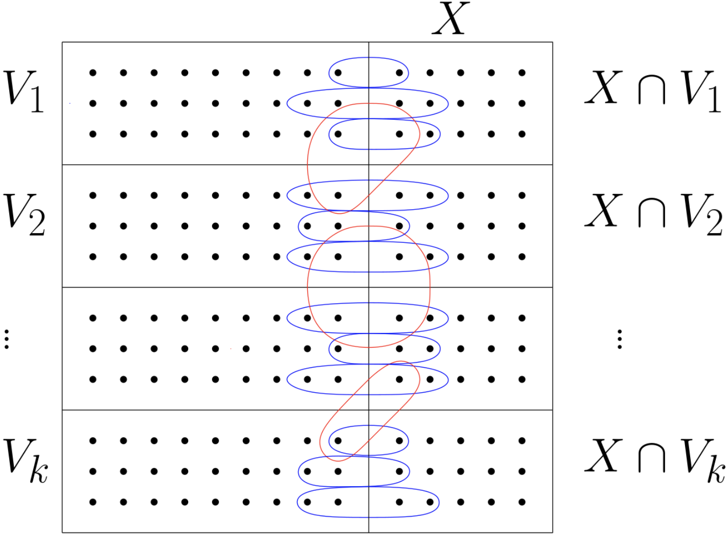
Figure 2. Comparison of $f_{c}$ and $g_{c}$

As Figure 2 shows, $g_{c}$ only counts the blue pairs while $f_{c}$ counts red pairs in addition. By virtue of the fact that there are fewer conditions imposed on the sets included in the count for $f_{c}$, we must have $f_{c}\geq g_{c}$. Thus, rewriting Equation B.11, we obtain

$$\mathbb{E}(|E_{m}(X,X^{c})|) \,=g_{c}\frac{a_{m}}{{n\choose m-1}}+(f_{c}-g_{c})\frac{b_{m}}{{n\choose m-1}}\,~{}.$$

Since both terms in the above sum are positive, we can upper bound by taking $a_{m}=b_{m}$ to obtain

$$\mathbb{E}\left(|E_{m}(X,X^{c})|\right)\leq f_{c}\frac{a_{m}}{{n\choose m-1}}=\Bigg{[}{n\choose m}-{cn\choose m}-{(1-c)n\choose m}\Bigg{]}\frac{a_{m}}{{n\choose m-1}}~{}.$$

By summing over $m$, the expectation of $\sum_{m=2}^{M}(m-1)^{2}|E_{m}(X,X^{c})|$ satisfies

$$\sum_{m=2}^{M}(m-1)^{2}\cdot\mathbb{E}\left(|E_{m}(X,X^{c})|\right) \leq\sum_{m=2}^{M}(m-1)^{2}\Bigg{[}{n\choose m}-{cn\choose m}-{(1-c)n\choose m}\Bigg{]}\frac{a_{m}}{{n\choose m-1}}~{},$$

$$\leq 2n\sum_{m=2}^{M}(1-c^{m}-(1-c)^{m})(m-1)a_{m}\leq 8Mcnd\,,$$

where the last upper inequality holds when $c\leq c_{0}=c_{0}(m)$ is sufficiently small, since

$$\,[(1-c)+c]^{m}-c^{m}-(1-c)^{m}$$

$$= \,\binom{m}{1}(1-c)^{m-1}c+\binom{m}{2}(1-c)^{m-2}c^{2}+\cdots+\binom{m}{m-1}(1-c)^{1}c^{m-1}$$

(B.13) $$\leq \,\binom{m}{1}c+\binom{m}{2}c^{2}+\cdots+\binom{m}{m-1}c^{m-1}\leq(1+c)^{m}-1\leq 2(1+mc-1)\leq 2mc\,.$$

Similarly, we apply Bernstein Lemma D.3 again with $K=M^{2}$, $\sigma^{2}\leq 8M^{3}cnd$ and obtain

$$\,\mathbb{P}\left(\sum_{m=2}^{M}(m-1)^{2}|E_{m}(X,X^{c})|\geq 16Mcnd\right)$$

(B.14) $$\leq\, \,\mathbb{P}\left(\sum_{m=2}^{M}(m-1)^{2}(|E_{m}(X,X^{c})|-\mathbb{E}|E_{m}(X,X^{c})|)\geq 8Mcnd\right)\leq\exp(-6cnd/M)\,.$$

By the binomial coefficient upper bound $\binom{n}{k}\leq(\frac{en}{k})^{k}$ for $1\leq k\leq n$, there are at most

(B.15) $$\binom{n}{cn}\leq\left(\frac{e}{c}\right)^{cn}=\exp(-c(\log c-1)n)$$

many subsets $X$ of size $|X|=cn$. Let $d$ be sufficiently large so that $d^{-3}\leq c_{0}$. Substituting $c=d^{-3}$ in Equation B.15, we have

$${n\choose d^{-3}n}\leq\exp\left[3d^{-3}\log(d)n\right].$$

Taking $c=d^{-3}$ in Equation B.8 and Equation B.14, we obtain

$$\mathbb{P}\left(\sum_{m=2}^{M}(m-1)(m|E_{m}(X)|+(m-1)|E_{m}(X,X^{c})|)\geq 20Md^{-2}n\right)\leq 2\exp(-2d^{-2}n/M)\,.$$

Taking a union bound over all possible $X$ with $|X|=d^{-3}n$, we obtain with probability at least $1-2\exp(3d^{-3}\log dn-2d^{-2}n/M)\leq 1-2\exp(-d^{-2}n/M)$, no more than $d^{-3}n$ many vertices have total row sum greater than $20Md$. Note that we have imposed the condition that $d^{-3}\leq c_{0}$ (as in Equation B.13), so $d$ needs to be sufficiently large. ∎

B.4. Proof of Lemma 5.8

Proof.

Note that ${\boldsymbol{\rm{U}}}$ is spanned by first $k$ singular vectors of $({\boldsymbol{\rm{A}}}_{1})_{{\mathcal{I}}_{1}}$. Let $\{{\boldsymbol{u}}_{i}\}_{i=1}^{k}$ be an orthonormal basis of the ${\boldsymbol{\rm{U}}}$, then the projection $P_{{\boldsymbol{\rm{U}}}}:=\sum_{l=1}^{k}\langle{\boldsymbol{u}}_{l},\cdot\,\rangle{\boldsymbol{u}}_{l}$. Let $k(i)$ index the membership of vertex $i$. For each fixed $i\in V_{k(i)}\cap Y_{2}\cap\{i_{1},\cdots,i_{s}\}$,

$$P_{{\boldsymbol{\rm{U}}}}{\boldsymbol{e}}_{i}= \,\sum_{l=1}^{k}\langle{\boldsymbol{u}}_{l},{\boldsymbol{e}}_{i}\rangle{\boldsymbol{u}}_{l},\quad\|P_{{\boldsymbol{\rm{U}}}}{\boldsymbol{e}}_{i}\|_{2}^{2}=\,\sum_{l=1}^{k}\langle{\boldsymbol{u}}_{l},{\boldsymbol{e}}_{i}\rangle^{2}.$$

As a consequence of independence between entries in ${\boldsymbol{\rm{A}}}_{1}$ and entries in ${\boldsymbol{\rm{A}}}_{2}$, defined in Equation 5.7, it is known that $\{{\boldsymbol{u}}_{l}\}_{l=1}^{k}$ and ${\boldsymbol{e}}_{i}$ are independent of each other, since ${\boldsymbol{e}}_{i}$ are columns of ${\boldsymbol{\rm{E}}}_{2}:={\boldsymbol{\rm{A}}}_{2}-\widetilde{{\boldsymbol{\rm{A}}}}_{2}$. If the expectation is taken over $\{\boldsymbol{\mathcal{T}}^{(m)}\}_{m\in\mathcal{M}}$ conditioning on $\{{\boldsymbol{u}}_{l}\}_{l=1}^{k}$, then

$$\mathbb{E}_{\{\boldsymbol{\mathcal{T}}^{(m)}\}_{m\in\mathcal{M}}}\left[\langle{\boldsymbol{u}}_{l},{\boldsymbol{e}}_{i}\rangle\Big{|}\{{\boldsymbol{u}}_{l}\}_{l=1}^{k}\right]= \,\sum_{j=1}^{n}{\boldsymbol{u}}_{l}(j)\cdot\mathbb{E}\left(\Big{[}({\boldsymbol{\rm{A}}}_{2})_{ji}-(\mathbb{E}{\boldsymbol{\rm{A}}}_{2})_{ji}\Big{]}\right)=0\,,$$

$$\mathbb{E}_{\{\boldsymbol{\mathcal{T}}^{(m)}\}_{m\in\mathcal{M}}}\left[\|P_{{\boldsymbol{\rm{U}}}}{\boldsymbol{e}}_{i}\|_{2}^{2}\Big{|}\{{\boldsymbol{u}}_{l}\}_{l=1}^{k}\right]= \,\sum_{l=1}^{k}\mathbb{E}_{\{\boldsymbol{\mathcal{T}}^{(m)}\}_{m\in\mathcal{M}}}\left[\langle{\boldsymbol{u}}_{l},{\boldsymbol{e}}_{i}\rangle^{2}\Big{|}\{{\boldsymbol{u}}_{l}\}_{l=1}^{k}\right]\,,$$

where $\mathcal{M}$ is obtained from Algorithm 1. Expand each $\langle{\boldsymbol{u}}_{l},{\boldsymbol{e}}_{i}\rangle^{2}$ and rewrite it into $2$ parts,

$$\langle{\boldsymbol{u}}_{l},{\boldsymbol{e}}_{i}\rangle^{2}= \,\sum_{j_{1}=1}^{k}\sum_{j_{2}=1}^{k}{\boldsymbol{u}}_{l}(j_{1}){\boldsymbol{e}}_{i}(j_{1}){\boldsymbol{u}}_{l}(j_{2}){\boldsymbol{e}}_{i}(j_{2})$$

(B.16) $$= \,\underbrace{\sum_{j=1}^{k}[{\boldsymbol{u}}_{l}(j)]^{2}[{\boldsymbol{e}}_{i}(j)]^{2}}_{(a)}+\underbrace{\sum_{j_{1}\neq j_{2}}{\boldsymbol{u}}_{l}(j_{1}){\boldsymbol{e}}_{i}(j_{1}){\boldsymbol{u}}_{l}(j_{2}){\boldsymbol{e}}_{i}(j_{2})}_{(b)}\,,\quad\forall l\in[k]\,.$$

Part $(a)$ is the contribution from graph, i.e., $2$-uniform hypergraph, while part $(b)$ is the contribution from $m$-uniform hypergraph with $m\geq 3$, which only occurs in hypergraph clustering. The expectation of part $(a)$ in is upper bounded by $\alpha$ as defined in Equation 2.4, since

$$\mathbb{E}_{\{\boldsymbol{\mathcal{T}}^{(m)}\}_{m\in\mathcal{M}}}\left[\sum_{j=1}^{k}[{\boldsymbol{u}}_{l}(j)]^{2}[{\boldsymbol{e}}_{i}(j)]^{2}\Bigg{|}\{{\boldsymbol{u}}_{l}\}_{l=1}^{k}\right]=\sum_{j=1}^{n}[{\boldsymbol{u}}_{l}(j)]^{2}\cdot\mathbb{V}\textnormal{ar}\Big{(}({\boldsymbol{\rm{A}}}_{2})_{ji}\Big{)}$$

$$\leq\, \sum_{j=1}^{n}[{\boldsymbol{u}}_{l}(j)]^{2}\cdot(\mathbb{E}{\boldsymbol{\rm{A}}}_{2})_{ji}\leq\alpha=\sum_{m\in\mathcal{M}}\Bigg{[}\binom{\frac{n}{k}-2}{m-2}\frac{a_{m}-b_{m}}{\binom{n}{m-1}}+\binom{n}{m-2}\frac{b_{m}}{\binom{n}{m-1}}\Bigg{]}$$

$$\leq\, \sum_{m\in\mathcal{M}}\binom{n}{m-2}\frac{a_{m}}{\binom{n}{m-1}}\leq\frac{2}{n}\sum_{m\in\mathcal{M}}(m-1)a_{m}=\frac{2d}{n},\quad\forall l\in[k]$$

where $\|{\boldsymbol{u}}_{l}\|_{2}^{2}=\sum_{j=1}^{n}[{\boldsymbol{u}}_{l}(j)]^{2}=1$. For part $(b)$,

$$\,\mathbb{E}_{\{\boldsymbol{\mathcal{T}}^{(m)}\}_{m\in\mathcal{M}}}\left[\sum_{j_{1}\neq j_{2}}{\boldsymbol{u}}_{l}(j_{1}){\boldsymbol{e}}_{i}(j_{1}){\boldsymbol{u}}_{l}(j_{2}){\boldsymbol{e}}_{i}(j_{2})\Bigg{|}\{{\boldsymbol{u}}_{l}\}_{l=1}^{k}\right]$$

$$= \,\sum_{j_{1}\neq j_{2}}{\boldsymbol{u}}_{l}(j_{1}){\boldsymbol{u}}_{l}(j_{2})\mathbb{E}\left[\Big{(}({\boldsymbol{\rm{A}}}_{2})_{j_{1}i}-(\mathbb{E}{\boldsymbol{\rm{A}}}_{2})_{j_{1}i}\Big{)}\Big{(}({\boldsymbol{\rm{A}}}_{2})_{j_{2}i}-(\mathbb{E}{\boldsymbol{\rm{A}}}_{2})_{j_{2}i}\Big{)}\right]$$

$$= \,\sum_{j_{1}\neq j_{2}}{\boldsymbol{u}}_{l}(j_{1}){\boldsymbol{u}}_{l}(j_{2})\mathbb{E}\Bigg{(}\sum_{m\in\mathcal{M}}\,\,\sum_{\begin{subarray}{c}e\in E_{m}[Y_{2}\cup Z]\\ \{i,j_{1}\}\subset e\end{subarray}}\,(\boldsymbol{\mathcal{T}}^{(m)}_{e}-\mathbb{E}\boldsymbol{\mathcal{T}}^{(m)}_{e})\Bigg{)}\Bigg{(}\sum_{m\in\mathcal{M}}\,\,\sum_{\begin{subarray}{c}e\in E_{m}[Y_{2}\cup Z]\\ \{i,j_{2}\}\subset e\end{subarray}}\,(\boldsymbol{\mathcal{T}}^{(m)}_{e}-\mathbb{E}\boldsymbol{\mathcal{T}}^{(m)}_{e})\Bigg{)}.$$

According to Definition 2.1 of the adjacency tensor, $\boldsymbol{\mathcal{T}}^{(m)}_{e_{1}}$ and $\boldsymbol{\mathcal{T}}^{(m)}_{e_{2}}$ are independent if hyperedge $e_{1}\neq e_{2}$, then only the terms with hyperedge $e\supset\{i,j_{1},j_{2}\}$ have nonzero contribution. Then the expectation of part $(b)$ can be rewritten as

$$\,\mathbb{E}_{\{\boldsymbol{\mathcal{T}}^{(m)}\}_{m\in\mathcal{M}}}\left[\sum_{j_{1}\neq j_{2}}{\boldsymbol{u}}_{l}(j_{1}){\boldsymbol{e}}_{i}(j_{1}){\boldsymbol{u}}_{l}(j_{2}){\boldsymbol{e}}_{i}(j_{2})\Bigg{|}\{{\boldsymbol{u}}_{l}\}_{l=1}^{k}\right]$$

$$= \,\sum_{j_{1}\neq j_{2}}{\boldsymbol{u}}_{l}(j_{1}){\boldsymbol{u}}_{l}(j_{2})\sum_{m\in\mathcal{M}}\,\,\sum_{\begin{subarray}{c}e\in E_{m}[Y_{2}\cup Z]\\ \{i,j_{1},j_{2}\}\subset e\end{subarray}}\mathbb{E}\big{(}\boldsymbol{\mathcal{T}}^{(m)}_{e}-\mathbb{E}\boldsymbol{\mathcal{T}}^{(m)}_{e}\big{)}^{2}$$

$$\leq \,\sum_{j_{1}\neq j_{2}}{\boldsymbol{u}}_{l}(j_{1}){\boldsymbol{u}}_{l}(j_{2})\sum_{m\in\mathcal{M}}\,\,\sum_{\begin{subarray}{c}e\in E_{m}[Y_{2}\cup Z]\\ \{i,j_{1},j_{2}\}\subset e\end{subarray}}\mathbb{E}\boldsymbol{\mathcal{T}}^{(m)}_{e}$$

(B.18) $$= \sum_{j_{1}\neq j_{2}}{\boldsymbol{u}}_{l}(j_{1}){\boldsymbol{u}}_{l}(j_{2})\sum_{m\in\mathcal{M}}\sum_{\begin{subarray}{c}e\in E_{m}[Y_{2}\cup Z]\\ \{i,j_{1},j_{2}\}\subset e\end{subarray}}\frac{a_{m}}{\binom{n}{m-1}}\,.$$

Note that $|Y_{2}\cup Z|\leq n$, then the number of possible hyperedges $e$, while $e\in E_{m}[Y_{2}\cup Z]$ and $e\supset\{i,j_{1},j_{2}\}$, is at most $\binom{n}{m-3}$. Thus Equation B.18 is upper bounded by

$$\,\sum_{j_{1}\neq j_{2}}{\boldsymbol{u}}_{l}(j_{1}){\boldsymbol{u}}_{l}(j_{2})\sum_{m\in\mathcal{M}}\binom{n}{m-3}\frac{a_{m}}{\binom{n}{m-1}}$$

$$\leq \,\sum_{j_{1}\neq j_{2}}{\boldsymbol{u}}_{l}(j_{1}){\boldsymbol{u}}_{l}(j_{2})\sum_{m\in\mathcal{M}}\frac{(m-1)(m-2)}{(n-m)^{2}}a_{m}\leq\frac{d\mathcal{M}_{\max}}{n^{2}}\sum_{j_{1}\neq j_{2}}{\boldsymbol{u}}_{l}(j_{1}){\boldsymbol{u}}_{l}(j_{2})\,$$

$$\leq \,\frac{d\mathcal{M}_{\max}}{2n^{2}}\sum_{j_{1}\neq j_{2}}\Big{(}[{\boldsymbol{u}}_{l}(j_{1})]^{2}+[{\boldsymbol{u}}_{l}(j_{2})]^{2}\Big{)}\leq\frac{d\mathcal{M}_{\max}(n-1)}{2n^{2}}\Bigg{(}\sum_{j_{1}=1}^{n}[{\boldsymbol{u}}_{l}(j_{1})]^{2}+\sum_{j_{2}=1}^{n}[{\boldsymbol{u}}_{l}(j_{2})]^{2}\Bigg{)}$$

$$\leq \frac{d\mathcal{M}_{\max}}{n}\,,$$

where $\|{\boldsymbol{u}}_{l}\|_{2}=1$, $d=\sum_{m\in\mathcal{M}}(m-1)a_{m}$. With the upper bounds for part $(a)$ and $(b)$ in Equation B.16, the conditional expectation of $\|P_{{\boldsymbol{\rm{U}}}}{\boldsymbol{e}}_{i}\|_{2}^{2}$ is bounded by

$$\mathbb{E}_{\{\boldsymbol{\mathcal{T}}^{(m)}\}_{m\in\mathcal{M}}}\left[\|P_{{\boldsymbol{\rm{U}}}}{\boldsymbol{e}}_{i}\|_{2}^{2}\Big{|}\{{\boldsymbol{u}}_{l}\}_{l=1}^{k}\right]= \,\sum_{l=1}^{k}\mathbb{E}_{\{\boldsymbol{\mathcal{T}}^{(m)}\}_{m\in\mathcal{M}}}\left[\langle{\boldsymbol{u}}_{l},{\boldsymbol{e}}_{i}\rangle^{2}\Big{|}\{{\boldsymbol{u}}_{l}\}_{l=1}^{k}\right]\leq\frac{kd}{n}(\mathcal{M}_{\max}+2)\,,$$

Let $X_{i}$ be the Bernoulli random variable defined by

$$X_{i}=\mathbbm{1}\{\|P_{{\boldsymbol{\rm{U}}}}{\boldsymbol{e}}_{i}\|_{2}>2\sqrt{kd(\mathcal{M}_{\max}+2)/n)}\}\,,\quad i\in\{i_{1},\cdots,i_{s}\}\,.$$

By Markov’s inequality,

$$\mathbb{E}X_{i}=\mathbb{P}\left(\|P_{{\boldsymbol{\rm{U}}}}{\boldsymbol{e}}_{i}\|_{2}>2\sqrt{kd(\mathcal{M}_{\max}+2)/n}\right)\leq\frac{\mathbb{E}_{\{\boldsymbol{\mathcal{T}}^{(m)}\}_{m\in\mathcal{M}}}\left[\|P_{{\boldsymbol{\rm{U}}}}{\boldsymbol{e}}_{i}\|_{2}^{2}\Big{|}\{{\boldsymbol{u}}_{l}\}_{l=1}^{k}\right]}{4kd(\mathcal{M}_{\max}+2)/n}\leq\frac{1}{4}\,.$$

Let $\delta:=\frac{s}{2\sum_{j=1}^{s}\mathbb{E}X_{i_{j}}}-1$ where $s=2k\log^{2}(n)$. By Hoeffding Lemma D.2,

$$\,\mathbb{P}\Bigg{(}\sum_{j=1}^{s}X_{i_{j}}\geq\frac{s}{2}\Bigg{)}=\mathbb{P}\Bigg{(}\sum_{j=1}^{s}(X_{i_{j}}-\mathbb{E}X_{i_{j}})\geq\delta\sum_{j=1}^{s}\mathbb{E}X_{i_{j}}\Bigg{)}$$

$$\leq \,\exp\Bigg{(}-\frac{2\delta^{2}\big{(}\sum_{j=1}^{s}\mathbb{E}X_{i_{j}}\big{)}^{2}}{s}\Bigg{)}=O\Bigg{(}\frac{1}{n^{k\log(n)}}\Bigg{)}\,.$$

Therefore, with probability $1-O(n^{-k\log(n)})$, at least $s/2$ of the vectors ${\boldsymbol{e}}_{i_{1}},\dots,{\boldsymbol{e}}_{i_{s}}$ satisfy

$$\|P_{{\boldsymbol{\rm{U}}}}{\boldsymbol{e}}_{i}\|_{2}\leq 2\sqrt{kd(\mathcal{M}_{\max}+2)/n}.$$

Meanwhile, for any $c\in(0,2)$, there exists some large enough constant $C_{2}\geq 2^{\mathcal{M}_{\max}+1}\sqrt{(\mathcal{M}_{\max}+2)/k}/c$ such that if $\sum_{m\in\mathcal{M}}(m-1)(a_{m}-b_{m})>C_{2}k^{\mathcal{M}_{\max}-1}\sqrt{d}$, then

$$\|\overline{{\boldsymbol{\delta}}}_{i}\|_{2}=\frac{\sqrt{n}(\bar{\alpha}-\bar{\beta})}{2}=\frac{\sqrt{n}}{2}\sum_{m\in\mathcal{M}}\binom{\frac{3n}{4k}-2}{m-2}\frac{a_{m}-b_{m}}{\binom{n}{m-1}}$$

$$=\, \frac{(1+o(1))}{2\sqrt{n}}\sum_{m\in\mathcal{M}}\Big{(}\frac{3}{4k}\Big{)}^{m-2}(m-1)(a_{m}-b_{m})\geq\frac{k}{(2k)^{\mathcal{M}_{\max}-1}\sqrt{n}}\sum_{m\in\mathcal{M}}(m-1)(a_{m}-b_{m}),$$

$$>\, \frac{C_{2}k^{\mathcal{M}_{\max}}\sqrt{d}}{(2k)^{\mathcal{M}_{\max}-1}\sqrt{n}}\geq\frac{2^{\mathcal{M}_{\max}+1}\sqrt{(\mathcal{M}_{\max}+2)}k^{\mathcal{M}_{\max}}\sqrt{d}}{c(2k)^{\mathcal{M}_{\max}-1}\sqrt{kn}}$$

$$> \frac{2}{c}~{}2\sqrt{\frac{kd(\mathcal{M}_{\max}+2)}{n}}>\frac{2}{c}\|P_{{\boldsymbol{\rm{U}}}}{\boldsymbol{e}}_{i}\|_{2}.$$

∎

B.5. Proof of Lemma 5.10

Proof.

Split $[n]$ into $V_{1}^{\prime}$ and $V_{2}^{\prime}$ such that $V_{1}^{\prime}=\{i|{\boldsymbol{v}}(i)>0\}$ and $V_{2}^{\prime}=\{i|{\boldsymbol{v}}(i)\leq 0\}$. Without loss of generality, assume that the first $\frac{n}{k}$ entries of $\bar{{\boldsymbol{v}}}$ are positive. We can write ${\boldsymbol{v}}$ in terms of its orthogonal projection onto $\bar{{\boldsymbol{v}}}$ as

(B.20) $${\boldsymbol{v}}=c_{1}\bar{{\boldsymbol{v}}}+{\boldsymbol{\varepsilon}}=\Big{[}{\boldsymbol{\varepsilon}}_{1}+\frac{c_{1}}{\sqrt{n}},\cdots,{\boldsymbol{\varepsilon}}_{\frac{n}{k}}+\frac{c_{1}}{\sqrt{n}},\,\,{\boldsymbol{\varepsilon}}_{\frac{n}{k}+1}-\frac{c_{1}}{\sqrt{n}},\cdots,{\boldsymbol{\varepsilon}}_{n}-\frac{c_{1}}{\sqrt{n}}\Big{]}^{{\mathsf{T}}}\,,$$

where $\bar{{\boldsymbol{v}}}\perp{\boldsymbol{\varepsilon}}$ with $\|{\boldsymbol{\varepsilon}}\|_{2}<c$ and $c_{1}\geq\sqrt{1-c^{2}}$. The number of entries of ${\boldsymbol{\varepsilon}}$ smaller than $-\frac{\sqrt{1-c^{2}}}{\sqrt{n}}$ is at most $\frac{c^{2}}{1-c^{2}}n$. Note that $c_{1}\geq\sqrt{1-c^{2}}$, so at least $\frac{n}{k}-\frac{c^{2}}{1-c^{2}}n$ indices $i$ with $\bar{{\boldsymbol{v}}}_{i}=\frac{1}{\sqrt{n}}$ will have ${\boldsymbol{v}}_{i}>0$, thus the ratio we are seeking is at least

$$\frac{\frac{n}{k}-\frac{c^{2}}{1-c^{2}}n}{\frac{n}{k}}=1-\frac{kc^{2}}{1-c^{2}}>1-\frac{4k}{3}c^{2}.$$

∎

B.6. Proof of Lemma 5.11

Proof.

We start with the following simple claim: for any $m\geq 2$ and any $\nu\in[1/2,1)$,

(B.21) $$\nu^{m}+(1-\nu)^{m}<\left(\frac{1+\nu}{2}\right)^{m}~{}.$$

Indeed, one quick way to see this is by induction on $m$; we will induct from $m$ to $m+2$. Assume the inequality is true for $m$; then

$$\nu^{m+2}+(1-\nu)^{m+2} = \nu^{2}\nu^{m}+(1-\nu)^{2}(1-\nu)^{m}$$

$$= \nu^{2}\nu^{m}+(1-2\nu+\nu^{2})(1-\nu)^{m}~{}\leq~{}\nu^{2}\nu^{m}+\nu^{2}(1-\nu)^{m}$$

$$= \nu^{2}(\nu^{m}+(1-\nu)^{m})~{}<~{}(\nu^{2}+(1-\nu)^{2})(\nu^{m}+(1-\nu)^{m})$$

$$< \left(\frac{1+\nu}{2}\right)^{2}\left(\frac{1+\nu}{2}\right)^{m}=\left(\frac{1+\nu}{2}\right)^{m+2}~{},$$

where we have used the induction hypothesis together with $1-2\nu\leq 0$ and $(1-\nu)^{2}>0$. After easily checking that the inequality works for $m=2,3$, the induction is complete. We shall now check that the quantities defined in Lemma 5.11 obey the relationship $\mu_{2}\geq\mu_{1}$ and $\mu_{2}-\mu_{1}=\Omega(n)$, for $n$ large enough. First, note that the only thing we need to check is that, for sufficiently large $n$,

$$\binom{\frac{\nu n}{2k}}{m}+\binom{\frac{(1-\nu)n}{2k}}{m}\leq\binom{\frac{(1+\nu)n}{4k}}{m}+(k-1)\binom{\frac{(1-\nu)n}{4k(k-1)}}{m}~{};$$

in fact, we will show the stronger statement that for any $m\geq 2$ and $n$ large enough,

(B.22) $$\binom{\frac{\nu n}{2k}}{m}+\binom{\frac{(1-\nu)n}{2k}}{m}<\binom{\frac{(1+\nu)n}{4k}}{m}~{},$$

and this will suffice to see that the second part of the assertion, $\mu_{2}-\mu_{1}=\Omega(n)$, is also true. Asymptotically, $\binom{\frac{\nu n}{2k}}{m}\sim\frac{\nu^{m}}{m!}\left(\frac{n}{2k}\right)^{m}$, $\binom{\frac{(1-\nu)n}{2k}}{m}\sim\frac{(1-\nu)^{m}}{m!}\left(\frac{n}{2k}\right)^{m}$, and $\binom{\frac{(1+\nu)n}{4k}}{m}\sim\frac{\left(\frac{1+\nu}{2}\right)^{m}}{m!}\left(\frac{n}{2k}\right)^{m}$. Note then that Equation B.22 follows from Equation B.21.

Let {$V_{1},\dots,V_{k}$} be the true partition of $V$. Recall that hyperedges in $H=\cup_{m\in\mathcal{M}}H_{m}$ are colored red and blue with equal probability in Algorithm 1. Let $E_{m}(X)$ denote the set of blue $m$-uniform hyperedges with all vertices located in the vertex set $X$. Assume $|X\cap V_{i}|=\eta_{i}|X|$ with $\sum_{i=1}^{k}\eta_{i}=1$. For each $m\in\mathcal{M}$, the presence of hyperedge $e\in E_{m}(X)$ can be represented by independent Bernoulli random variables

$$T_{e}^{(a_{m})}\sim\mathrm{Bernoulli}\left(\frac{a_{m}}{2\binom{n}{m-1}}\right),\quad T_{e}^{(b_{m})}\sim\mathrm{Bernoulli}\left(\frac{b_{m}}{2\binom{n}{m-1}}\right)\,,$$

depending on whether $e$ is a hyperedge with all vertices in the same block. Denote by

$$E_{m}(X,a_{m}):=\cup_{i=1}^{k}E_{m}(V_{i}\cap X)$$

the union of all $m$-uniform sets of hyperedges with all vertices in the same $V_{i}\cap X$ for some $i\in[k]$, and by

$$E_{m}(X,b_{m}):=\,E_{m}(X)\setminus E_{m}(X,a_{m})=E_{m}(X)\setminus\Big{(}\cup_{i}^{k}E_{m}(V_{i}\cap X)\Big{)}$$

the set of $m$-uniform hyperedges with vertices across different blocks $V_{i}\cap X$. Then the cardinality $|E_{m}(X)|$ can be written as the

$$|E_{m}(X)|=\sum_{e\in E_{m}(X,a_{m})}T_{e}^{(a_{m})}\,+\sum_{e\in E_{m}(X,b_{m})}T_{e}^{(b_{m})}\,,$$

and by summing over $m$, the weighted cardinality $|E(X)|$ is written as

$$|E(X)|:=\sum_{m\in\mathcal{M}}m(m-1)|E_{m}(X)|=\sum_{m\in\mathcal{M}}m(m-1)\left\{\sum_{e\in E_{m}(X,a_{m})}T_{e}^{(a_{m})}\,+\sum_{e\in E_{m}(X,b_{m})}T_{e}^{(b_{m})}\right\}\,,$$

with its expectation

(B.23) $$\mathbb{E}|E(X)|=\sum_{m\in\mathcal{M}}m(m-1)\left\{\sum_{i=1}^{k}\binom{\eta_{i}\frac{n}{2k}}{m}\frac{a_{m}-b_{m}}{2\binom{n}{m-1}}+\binom{\frac{n}{2k}}{m}\frac{b_{m}}{2\binom{n}{m-1}}\right\}\,,$$

since

$$|E_{m}(X,a_{m})|=\sum_{i=1}^{k}|E_{m}(V_{i}\cap X)|=\sum_{i=1}^{k}\binom{\eta_{i}\frac{n}{2k}}{m}\,,\quad|E_{m}(X,b_{m})|=\binom{\frac{n}{2k}}{m}-\sum_{i=1}^{k}\binom{\eta_{i}\frac{n}{2k}}{m}\,,$$

Next, we prove the two Statements in Lemma 5.11 separately. First, assume that $|X\cap V_{i}|\leq\nu|X|$ ( i.e., $\eta_{i}\leq\nu$) for each $i\in[k]$. Then

$$\mathbb{E}|E(X)|\leq \,\frac{1}{2}\sum_{m\in\mathcal{M}}m(m-1)\left\{\left[\binom{\frac{\nu n}{2k}}{m}+\binom{\frac{(1-\nu)n}{2k}}{m}\right]\frac{a_{m}-b_{m}}{\binom{n}{m-1}}+\binom{\frac{n}{2k}}{m}\frac{b_{m}}{\binom{n}{m-1}}\right\}=:\mu_{1}\,.$$

To justify the above inequality, note that since $\sum\limits_{i=1}^{k}\eta_{i}=1$, the sum $\sum_{i=1}^{k}\binom{\eta_{i}\frac{n}{2k}}{m}$ is maximized when all but $2$ of the $\eta_{i}$ are $0$, and since all $\eta_{i}\leq\nu$, this means that

$$\sum_{i=1}^{k}\binom{\eta_{i}\frac{n}{2k}}{m}\leq\binom{\frac{\nu n}{2k}}{m}+\binom{\frac{(1-\nu)n}{2k}}{m}\,.$$

Note that $m(m-1)(T_{e}^{(a_{m})}-\mathbb{E}T_{e}^{(a_{m})})$ and $m(m-1)(T_{e}^{(b_{m})}-\mathbb{E}T_{e}^{(b_{m})})$ are independent mean-zero random variables bounded by $M(M-1)$ for all $m\in\mathcal{M}$, and $\mathbb{V}\textnormal{ar}(|E(X)|)\leq M^{2}(M-1)^{2}\mathbb{E}|E(X)|=\Omega(n)$. Recall that $\mu_{\mathrm{T}}:=(\mu_{1}+\mu_{2})/2$. Define $t=\mu_{\mathrm{T}}-\mathbb{E}|E(X)|$, then $0<(\mu_{2}-\mu_{1})/2\leq t\leq\mu_{\mathrm{T}}$, hence $t=\Omega(n)$. By Bernstein’s Lemma D.3, we have

$$\mathbb{P}\Big{(}|E(X)|\geq\mu_{\mathrm{T}}\Big{)}=\mathbb{P}\Big{(}|E(X)|-\mathbb{E}|E(X)|\geq t\Big{)}\leq \exp\left(-\frac{t^{2}/2}{\mathbb{V}\textnormal{ar}(|E(X)|)+M(M-1)t/3}\right)=O(e^{-cn})\,,$$

where $c>0$ is some constant. On the other hand, if $|X\cap V_{i}|\geq\frac{1+\nu}{2}|X|$ for some $i\in[k]$, then

$$\,\mathbb{E}|E(X)|\geq\frac{1}{2}\sum_{m\in\mathcal{M}}m(m-1)\left\{\left[\binom{\frac{(1+\nu)n}{4k}}{m}+(k-1)\binom{\frac{(1-\nu)n}{4k(k-1)}}{m}\right]\frac{a_{m}-b_{m}}{\binom{n}{m-1}}+\binom{\frac{n}{2k}}{m}\frac{b_{m}}{\binom{n}{m-1}}\right\}=:\mu_{2}\,.$$

The above can be justified by noting that at least one $|X\cap V_{i}|\geq\frac{1+\nu}{2}|X|$, and that the rest of the vertices will yield a minimal binomial sum when they are evenly split between the remaining $V_{j}$. Similarly, define $t=\mu_{\mathrm{T}}-\mathbb{E}|E(X)|$, then $0<(\mu_{2}-\mu_{1})/2\leq-t=\Omega(n)$, and Bernstein’s Lemma D.3 gives

$$\mathbb{P}\Big{(}|E(X)|\leq\mu_{\mathrm{T}}\Big{)}= \,\mathbb{P}\Big{(}|E(X)|-\mathbb{E}|E(X)|\leq-t\Big{)}$$

$$\leq \,\exp\left(-\frac{t^{2}/2}{\mathbb{V}\textnormal{ar}(|E(X)|)+M(M-1)(-t)/3}\right)=O(e^{-c^{\prime}n})\,,$$

where $c^{\prime}>0$ is some other constant. ∎

B.7. Proof of Lemma 5.13

Proof.

If vertex $i$ is uniformly chosen from $Y_{2}$, the probability that $i\notin V_{l}$ for some $l\in[k]$ is

$$\mathbb{P}(i\notin V_{l}|i\in Y_{2})=\frac{\mathbb{P}(i\notin V_{l},i\in Y_{2})}{\mathbb{P}(i\in Y_{2})}=1-\frac{|V_{l}\cap Y_{2}|}{|Y_{2}|}=1-\frac{\frac{n}{k}-n_{l}-n^{\prime}_{l}}{n-\sum_{t=1}^{k}(n_{t}+n_{t}^{\prime})}\,,\quad l\in[k]\,,$$

where $n_{t}$ and $n_{t}^{\prime}$, defined in Equation 5.1 and Equation 5.2, denote the cardinality of $Z\cap V_{t}$ and $Y_{1}\cap V_{t}$ respectively. As proved in Section B.2, with probability at least $1-2\exp(-k\log^{2}(n))$, we have

$$|n_{t}-n/(2k)|\leq\sqrt{n}\log(n)~{}\text{ and }~{}|n_{t}^{\prime}-n/(4k)|\leq\sqrt{n}\log(n),$$

then $\mathbb{P}(i\notin V_{l}|i\in Y_{2})=1-\frac{1}{k}\Big{(}1+o(1)\Big{)}\,.$ After $k\log^{2}n$ samples from $Y_{2}$, the probability that there exists at least one node which belongs to $V_{l}$ is at least

$$1-\bigg{(}1-\frac{1+o(1)}{k}\bigg{)}^{k\log^{2}n}=1-n^{-(1+o(1))k\log(\frac{k}{k-1})\log n}.$$

The proof is completed by a union bound over $l\in[k]$.

∎

B.8. Proof of Lemma 5.14

Proof.

We calculate $\mathbb{P}(S_{11}^{\prime}(u)\leq\mu_{\rm{C}})$ first. Define $t_{\rm{1C}}:=\mu_{\rm{C}}-\mathbb{E}S_{11}^{\prime}(u)$, then by Bernstein’s inequality (Lemma D.3) and taking $K=\mathcal{M}_{\max}-1$,

$$\,\mathbb{P}\left(S_{11}^{\prime}(u)\leq\mu_{\rm{C}}\right)=\mathbb{P}\left(S^{\prime}_{11}(u)-\mathbb{E}S^{\prime}_{11}(u)\leq t_{\rm{1C}}\right)$$

$$\leq \,\exp\left(-\frac{t_{\rm{1C}}^{2}/2}{\mathbb{V}\textnormal{ar}[S_{11}^{\prime}(u)]+(\mathcal{M}_{\max}-1)\cdot t_{\rm{1C}}/3}\right)\leq\exp\left(-\frac{3t_{\rm{1C}}^{2}/(\mathcal{M}_{\max}-1)}{6(\mathcal{M}_{\max}-1)\cdot\mathbb{E}S_{11}^{\prime}(u)+2t_{\rm{1C}}}\right)$$

$$\leq \,\exp\left(-\frac{[(\nu)^{\mathcal{M}_{\max}-1}-(1-\nu)^{\mathcal{M}_{\max}-1}]^{2}}{(\mathcal{M}_{\max}-1)^{2}\cdot 2^{2\mathcal{M}_{\max}+3}}\cdot\frac{\left[\sum_{m\in\mathcal{M}}(m-1)\left(\frac{a_{m}-b_{m}}{k^{m-1}}\right)\right]^{2}}{\sum_{m\in\mathcal{M}}(m-1)\left(\frac{a_{m}-b_{m}}{k^{m-1}}+b_{m}\right)}\right)\,,$$

where $\mathcal{M}$ is obtained from Algorithm 1 with $\mathcal{M}_{\max}$ denoting the maximum value in $\mathcal{M}$, and the last two inequalities hold since $\mathbb{V}\textnormal{ar}[S_{11}^{\prime}(u)]\leq(\mathcal{M}_{\max}-1)^{2}\mathbb{E}S_{11}^{\prime}(u)$, and for sufficiently large $n$,

$$t_{\rm{1C}}:= \,\mu_{\rm{C}}-\mathbb{E}S_{11}^{\prime}(u)=-\frac{1}{2}\sum_{m\in\mathcal{M}}(m-1)\cdot\left[\binom{\frac{\nu n}{2k}}{m-1}-\binom{\frac{(1-\nu)n}{2k}}{m-1}\right]\frac{a_{m}-b_{m}}{2\binom{n}{m-1}}$$

$$\leq \,-\frac{1}{2}\sum_{m\in\mathcal{M}}\frac{(\nu)^{m-1}-(1-\nu)^{m-1}}{2^{m}}\cdot(m-1)\frac{a_{m}-b_{m}}{k^{m-1}}(1+o(1))$$

$$\leq \,-\frac{(\nu)^{\mathcal{M}_{\max}-1}-(1-\nu)^{\mathcal{M}_{\max}-1}}{2^{\mathcal{M}_{\max}+2}}\sum_{m\in\mathcal{M}}(m-1)\cdot\frac{a_{m}-b_{m}}{k^{m-1}}\,,$$

$$\,6(\mathcal{M}_{\max}-1)\mathbb{E}S_{11}^{\prime}(u)+2t_{\rm{1C}}=2\mu_{\rm{C}}+(6\mathcal{M}_{\max}-8)\mathbb{E}S^{\prime}_{11}(u)$$

$$= \,\sum_{m\in\mathcal{M}}(m-1)\left\{\left[(6\mathcal{M}_{\max}-7)\binom{\frac{\nu n}{2k}}{m-1}+\binom{\frac{(1-\nu)n}{2k}}{m-1}\right]\frac{a_{m}-b_{m}}{2\binom{n}{m-1}}+6(\mathcal{M}_{\max}-1)\binom{\frac{n}{2k}}{m-1}\frac{b_{m}}{2\binom{n}{m-1}}\right\}$$

$$= \,\sum_{m\in\mathcal{M}}(m-1)\left[\frac{(6\mathcal{M}_{\max}-7)\cdot(\nu)^{m-1}+(1-\nu)^{m-1}}{2^{m}}\cdot\frac{a_{m}-b_{m}}{k^{m-1}}+\frac{(6\mathcal{M}_{\max}-6)b_{m}}{2^{m}k^{m-1}}\right](1+o(1))$$

$$\leq \,\sum_{m\in\mathcal{M}}\frac{(6\mathcal{M}_{\max}-7)\cdot(\nu)^{m-1}+(1-\nu)^{m-1}}{2^{m}}\cdot(m-1)\left(\frac{a_{m}-b_{m}}{k^{m-1}}+b_{m}\right)(1+o(1))$$

$$\leq \,\frac{3(\mathcal{M}_{\max}-1)}{2}\sum_{m\in\mathcal{M}}(m-1)\left(\frac{a_{m}-b_{m}}{k^{m-1}}+b_{m}\right)\,.$$

Similarly, for $\mathbb{P}(S_{1j}^{\prime}(u)\geq\mu_{\rm{C}})$, define $t_{\rm{jC}}:=\mu_{\rm{C}}-\mathbb{E}S_{1j}^{\prime}(u)$ for $j\neq 1$, by Bernstein’s Lemma D.3,

$$\,\mathbb{P}\left(S_{1j}^{\prime}(u)\geq\mu_{\rm{C}}\right)=\mathbb{P}\left(S^{\prime}_{1j}(u)-\mathbb{E}S^{\prime}_{1j}(u)\geq t_{\rm{jC}}\right)$$

$$\leq \,\exp\left(-\frac{t_{\rm{jC}}^{2}/2}{\mathbb{V}\textnormal{ar}[S_{1j}^{\prime}(u)]+(\mathcal{M}_{\max}-1)\cdot t_{\rm{jC}}/3}\right)\leq\exp\left(-\frac{3t_{\rm{jC}}^{2}/(\mathcal{M}_{\max}-1)}{6(\mathcal{M}_{\max}-1)\cdot\mathbb{E}S_{1j}^{\prime}(u)+2t_{\rm{jC}}}\right)$$

$$\leq \,\exp\left(-\frac{[(\nu)^{\mathcal{M}_{\max}-1}-(1-\nu)^{\mathcal{M}_{\max}-1}]^{2}}{(\mathcal{M}_{\max}-1)^{2}\cdot 2^{2\mathcal{M}_{\max}+3}}\cdot\frac{\left[\sum_{m\in\mathcal{M}}(m-1)\left(\frac{a_{m}-b_{m}}{k^{m-1}}\right)\right]^{2}}{\sum_{m\in\mathcal{M}}(m-1)\left(\frac{a_{m}-b_{m}}{k^{m-1}}+b_{m}\right)}\right)\,.$$

The last two inequalities holds since $\mathbb{V}\textnormal{ar}[S_{1j}^{\prime}(u)]\leq(\mathcal{M}_{\max}-1)^{2}\mathbb{E}S_{1j}^{\prime}(u)$, and for sufficiently large $n$,

$$t_{\rm{jC}}:= \,\mu_{\rm{C}}-\mathbb{E}S_{1j}^{\prime}(u)=\frac{1}{2}\sum_{m\in\mathcal{M}}(m-1)\cdot\left[\binom{\frac{\nu n}{2k}}{m-1}-\binom{\frac{(1-\nu)n}{2k}}{m-1}\right]\frac{a_{m}-b_{m}}{2\binom{n}{m-1}}$$

$$\geq \,\frac{(\nu)^{\mathcal{M}_{\max}-1}-(1-\nu)^{\mathcal{M}_{\max}-1}}{2^{\mathcal{M}_{\max}+2}}\sum_{m\in\mathcal{M}}(m-1)\cdot\frac{a_{m}-b_{m}}{k^{m-1}}\,\,,$$

$$\,6\mathbb{E}S_{1j}^{\prime}(u)+2t_{\rm{jC}}=2\mu_{\rm{C}}+(6\mathcal{M}_{\max}-8)\mathbb{E}S^{\prime}_{1j}(u)$$

$$= \,\sum_{m\in\mathcal{M}}(m-1)\left\{\left[\binom{\frac{\nu n}{2k}}{m-1}+(6\mathcal{M}_{\max}-7)\binom{\frac{(1-\nu)n}{2k}}{m-1}\right]\frac{a_{m}-b_{m}}{2\binom{n}{m-1}}+6(\mathcal{M}_{\max}-1)\binom{\frac{n}{2k}}{m-1}\frac{b_{m}}{2\binom{n}{m-1}}\right\}$$

$$= \,\sum_{m\in\mathcal{M}}(m-1)\cdot\left(\frac{(\nu)^{m-1}+(6\mathcal{M}_{\max}-7)\cdot(1-\nu)^{m-1}}{2^{m}}\cdot\frac{a_{m}-b_{m}}{k^{m-1}}+\frac{(6\mathcal{M}_{\max}-6)\cdot b_{m}}{2^{m}k^{m-1}}\right)(1+o(1))$$

$$\leq \,\sum_{m\in\mathcal{M}}\frac{(\nu)^{m-1}+(6\mathcal{M}_{\max}-7)\cdot(1-\nu)^{m-1}}{2^{m}}\cdot(m-1)\left(\frac{a_{m}-b_{m}}{k^{m-1}}+b_{m}\right)(1+o(1))$$

$$\leq \,\frac{3(\mathcal{M}_{\max}-1)}{2}\sum_{m\in\mathcal{M}}(m-1)\left(\frac{a_{m}-b_{m}}{k^{m-1}}+b_{m}\right).$$

∎

Appendix C Algorithm correctness for the binary case

We will show the correctness of Algorithm 2 and prove Theorem 1.6 in this section. The analysis will mainly follow from the analysis in Section 5. We only detail the differences.

Without loss of generality, we assume $n$ is even to guarantee the existence of a binary partition of size $n/2$. The method to deal with the odd $n$ case was discussed in Lemma 2.4. Then, let the index set be ${\mathcal{I}}=\{i\in[n]:\mathrm{row}(i)\leq 20\mathcal{M}_{\max}d\}$, as shown in Equation 3.3. Let ${\boldsymbol{u}}_{i}$ (resp. $\bar{{\boldsymbol{u}}}_{i}$) denote the eigenvector associated to $\lambda_{i}({\boldsymbol{\rm{A}}}_{{\mathcal{I}}})$ (resp. $\lambda_{i}(\overline{{\boldsymbol{\rm{A}}}})$) for $i=1,2$. Define two linear subspaces ${\boldsymbol{\rm{U}}}:=\mathrm{Span}\{{\boldsymbol{u}}_{1},{\boldsymbol{u}}_{2}\}$ and $\overline{{\boldsymbol{\rm{U}}}}:=\mathrm{Span}\{\bar{{\boldsymbol{u}}}_{1},\bar{{\boldsymbol{u}}}_{2}\}$, then the angle between ${\boldsymbol{\rm{U}}}$ and $\overline{{\boldsymbol{\rm{U}}}}$ is defined as $\sin\angle({\boldsymbol{\rm{U}}},\overline{{\boldsymbol{\rm{U}}}}):=\|P_{{\boldsymbol{\rm{U}}}}-P_{\overline{{\boldsymbol{\rm{U}}}}}\|$, where $P_{{\boldsymbol{\rm{U}}}}$ and $P_{\overline{{\boldsymbol{\rm{U}}}}}$ are the orthogonal projections onto ${\boldsymbol{\rm{U}}}$ and $\overline{{\boldsymbol{\rm{U}}}}$, respectively.

C.1. Proof of Lemma 4.4

The strategy to bound the angle is similar to Section 5.1.2, except that we apply Davis-Kahan Theorem (Lemma D.6) here.

Define ${\boldsymbol{\rm{E}}}:={\boldsymbol{\rm{A}}}-\overline{{\boldsymbol{\rm{A}}}}$ and its restriction on ${\mathcal{I}}$, namely ${\boldsymbol{\rm{E}}}_{{\mathcal{I}}}:=({\boldsymbol{\rm{A}}}-\overline{{\boldsymbol{\rm{A}}}})_{{\mathcal{I}}}={\boldsymbol{\rm{A}}}_{{\mathcal{I}}}-\overline{{\boldsymbol{\rm{A}}}}_{{\mathcal{I}}}$, as well as ${\boldsymbol{\Delta}}:=\overline{{\boldsymbol{\rm{A}}}}_{{\mathcal{I}}}-\overline{{\boldsymbol{\rm{A}}}}$. Then the deviation ${\boldsymbol{\rm{A}}}_{{\mathcal{I}}}-\overline{{\boldsymbol{\rm{A}}}}$ is decomposed as

$${\boldsymbol{\rm{A}}}_{{\mathcal{I}}}-\overline{{\boldsymbol{\rm{A}}}}=({\boldsymbol{\rm{A}}}_{{\mathcal{I}}}-\overline{{\boldsymbol{\rm{A}}}}_{{\mathcal{I}}})+(\overline{{\boldsymbol{\rm{A}}}}_{{\mathcal{I}}}-\overline{{\boldsymbol{\rm{A}}}})={\boldsymbol{\rm{E}}}_{{\mathcal{I}}}+{\boldsymbol{\Delta}}\,.$$

Theorem 3.3 indicates $\|{\boldsymbol{\rm{E}}}_{{\mathcal{I}}}\|\leq C_{3}\sqrt{d}$ with probability at least $1-n^{-2}$ when taking $\tau=20\mathcal{M}_{\max},K=3$, where $C_{3}$ is a constant depending only on $\mathcal{M}_{\max}$. Moreover, Lemma 5.4 shows that the number of vertices with high degrees is relatively small. Consequently, an argument similar to Corollary 5.5 leads to the conclusion $\|{\boldsymbol{\Delta}}\|\leq\sqrt{d}$ w.h.p. Together with upper bounds for $\|{\boldsymbol{\rm{E}}}_{{\mathcal{I}}}\|$ and $\|{\boldsymbol{\Delta}}\|$, Lemma C.1 shows that the angle between ${\boldsymbol{\rm{U}}}$ and $\overline{{\boldsymbol{\rm{U}}}}$ is relatively small w.h.p.

Lemma C.1.

For any $c\in(0,1)$, there exists a constant $C_{2}$ depending on $\mathcal{M}_{\max}$ and $c$ such that if

$$\sum_{m\in\mathcal{M}}(m-1)(a_{m}-b_{m})\geq C_{2}\cdot 2^{\mathcal{M}_{\max}+2}\sqrt{d},$$

then $\sin\angle({\boldsymbol{\rm{U}}},\overline{{\boldsymbol{\rm{U}}}})\leq c$ with probability $1-n^{-2}$.

Proof.

First, with probability $1-n^{-2}$, we have

$$\|{\boldsymbol{\rm{A}}}_{{\mathcal{I}}}-\overline{{\boldsymbol{\rm{A}}}}\|\leq\|{\boldsymbol{\rm{E}}}_{{\mathcal{I}}}\|+\|{\boldsymbol{\Delta}}\|\leq(C_{3}+1)\sqrt{d}.$$

According to the definitions in Equation 2.4, $\alpha\geq\beta$ and $\alpha=O(1/n)$, $\beta=O(1/n)$. Meanwhile, Lemma 2.3 shows that $|\lambda_{2}(\overline{{\boldsymbol{\rm{A}}}})|=[-\alpha+(\alpha-\beta)n/2]$ and $|\lambda_{3}(\overline{{\boldsymbol{\rm{A}}}})|=\alpha$. Then

$$\,|\lambda_{2}(\overline{{\boldsymbol{\rm{A}}}})|-|\lambda_{3}(\overline{{\boldsymbol{\rm{A}}}})|=\frac{n}{2}(\alpha-\beta)-2\alpha\geq\frac{3}{4}\cdot\frac{n}{2}(\alpha-\beta)=\frac{3n}{8}\sum_{m\in\mathcal{M}}\binom{\frac{n}{2}-2}{m-2}\frac{(a_{m}-b_{m})}{\binom{n}{m-1}}$$

$$\geq \,\frac{1}{4}\sum_{m\in\mathcal{M}}\frac{(m-1)(a_{m}-b_{m})}{2^{m-2}}\geq\frac{1}{2^{\mathcal{M}_{\max}}}\sum_{m\in\mathcal{M}}(m-1)(a_{m}-b_{m})\geq 4C_{2}\sqrt{d}\,.$$

Then for some large enough $C_{2}$, the following condition for Davis-Kahan Theorem (Lemma D.6) is satisfied

$$\|{\boldsymbol{\rm{A}}}_{{\mathcal{I}}}-\overline{{\boldsymbol{\rm{A}}}}\|\leq(1-1/\sqrt{2})\left(|\lambda_{2}(\overline{{\boldsymbol{\rm{A}}}})|-|\lambda_{3}(\overline{{\boldsymbol{\rm{A}}}})|\right).$$

Then for any $c\in(0,1)$, we can choose $C_{2}=(C_{3}+1)/c$ such that

$$\|P_{{\boldsymbol{\rm{U}}}}-P_{\overline{{\boldsymbol{\rm{U}}}}}\|\leq\frac{2\|{\boldsymbol{\rm{A}}}_{{\mathcal{I}}}-\overline{{\boldsymbol{\rm{A}}}}\|}{|\lambda_{2}(\overline{{\boldsymbol{\rm{A}}}})|-|\lambda_{3}(\overline{{\boldsymbol{\rm{A}}}})|}\leq\frac{2(C_{3}+1)\sqrt{d}}{4C_{2}\sqrt{d}}=\frac{c}{2}\leq c\,.$$

∎

Now, we focus on the accuracy of Algorithm 5, once the conditions in Lemma C.1 are satisfied.

Lemma C.2 (Lemma 23 in [18]).

If $\sin\angle(\overline{{\boldsymbol{\rm{U}}}},{\boldsymbol{\rm{U}}})\leq c\leq\frac{1}{4}$, there exists a unit vector ${\boldsymbol{v}}\in{\boldsymbol{\rm{U}}}$ such that the angle between $\bar{{\boldsymbol{u}}}_{2}$ and ${\boldsymbol{v}}$ satisfies $\sin\angle(\bar{{\boldsymbol{u}}}_{2},{\boldsymbol{v}})\leq 2\sqrt{c}$.

The desired vector ${\boldsymbol{v}}$, as constructed in Algorithm 5, is the unit vector perpendicular to $P_{{\boldsymbol{\rm{U}}}}\mathbf{1}_{n}$, where $P_{{\boldsymbol{\rm{U}}}}\mathbf{1}_{n}$ is the projection of all-ones vector onto ${\boldsymbol{\rm{U}}}$. Lemma C.1 and Lemma C.2 together give the following corollary.

Corollary C.3.

For any $c\in(0,1)$, there exists a unit vector ${\boldsymbol{v}}\in{\boldsymbol{\rm{U}}}$ such that the angle between $\bar{{\boldsymbol{u}}}_{2}$ and ${\boldsymbol{v}}$ satisfies $\sin\angle(\bar{{\boldsymbol{u}}}_{2},{\boldsymbol{v}})\leq c<1$ with probability $1-O(e^{-n})$.

Proof.

For any $c\in(0,1)$, we could choose constants $C_{2}$, $C_{3}$ in Lemma C.1 such that $\sin\angle(\overline{{\boldsymbol{\rm{U}}}},{\boldsymbol{\rm{U}}})\leq\frac{c^{2}}{4}<1$. Then by Lemma C.2, we construct ${\boldsymbol{v}}$ such that $\sin\angle(\bar{{\boldsymbol{u}}}_{2},{\boldsymbol{v}})\leq c$. ∎

Lemma C.4 (Lemma $23$ in [18]).

If $\sin\angle(\bar{{\boldsymbol{u}}}_{2},{\boldsymbol{v}})<c\leq 0.5$, then we can identify at least $(1-8c^{2}/3)n$ vertices from each block correctly.

The proof of Lemma 4.4 is completed when choosing $C_{2}$, $C_{3}$ in Lemma C.1 s.t. $c\leq\frac{1}{4}$.

C.2. Proof of Lemma 4.5

The proof strategy is similar to Section 5.2 and Section 5.3. In Algorithm 2, we first color the hyperedges with red and blue with equal probability. By running Algorithm 6 on the red graph, we obtain a $\nu$-correct partition $V_{1}^{\prime},V_{2}^{\prime}$ of $V=V_{1}\cup V_{2}$, i.e., $|V_{l}\cap V_{l}^{\prime}|\geq\nu n/2$ for $l=1,2$. In the rest of the proof, we condition on this event and the event that the maximum red degree of a vertex is at most $\log^{2}(n)$ with probability at least $1-o(1)$. This can be proved by Bernstein’s inequality (Lemma D.3).

Similarly, we consider the probability of a hyperedge $e=\{i_{1},\cdots,i_{m}\}$ being blue conditioning on the event that $e$ is not a red hyperedge in each underlying $m$-uniform hypergraph separately. If vertices $i_{1},\cdots,i_{m}$ are all from the same true cluster, then the probability is $\psi_{m}$, otherwise $\phi_{m}$, where $\psi_{m}$ and $\phi_{m}$ are defined in Equation 5.25 and Equation 5.26, and the presence of those hyperedges are represented by random variables $\zeta_{e}^{(a_{m})}\sim\mathrm{Bernoulli}\left(\psi_{m}\right)$, $\xi_{e}^{(b_{m})}\sim\mathrm{Bernoulli}\left(\phi_{m}\right)$, respectively.

Following a similar argument in Section 5.2, the row sum of $u$ can be written as

$$S^{\prime}_{lj}(u):=\sum_{m\in\mathcal{M}}(m-1)\cdot\left\{\sum_{e\in\,\mathcal{E}^{(a_{m})}_{l,j}}\zeta_{e}^{(a_{m})}+\sum_{e\in\mathcal{E}^{(b_{m})}_{l,j}}\xi_{e}^{(b_{m})}\right\}\,,\quad u\in V_{l}\,,$$

where $\mathcal{E}^{(a_{m})}_{l,j}:=E_{m}([V_{l}]^{1},[V_{l}\cap V^{\prime}_{j}]^{m-1})$ denotes the set of $m$-hyperedges with $1$ vertex from $[V_{l}]^{1}$ and the other $m-1$ vertices from $[V_{l}\cap V^{\prime}_{j}]^{m-1}$, while $\mathcal{E}^{(b_{m})}_{l,j}:=E_{m}\Big{(}[V_{l}]^{1},\,\,[V^{\prime}_{j}]^{m-1}\setminus[V_{l}\cap V^{\prime}_{j}]^{m-1}\Big{)}$ denotes the set of $m$-hyperedges with $1$ vertex in $[V_{l}]^{1}$ while the remaining $m-1$ vertices in $[V^{\prime}_{j}]^{m-1}\setminus[V_{l}\cap V^{\prime}_{j}]^{m-1}$, with their cardinalities

$$|\mathcal{E}^{(a_{m})}_{l,j}|\leq\binom{|V_{l}\cap V^{\prime}_{j}|}{m-1}\,,\quad|\mathcal{E}^{(b_{m})}_{l,j}|\leq\left[\binom{|V^{\prime}_{j}|}{m-1}-\binom{|V_{l}\cap V^{\prime}_{j}|}{m-1}\right]\,.$$

According to the fact $|V_{l}\cap V_{l}^{\prime}|\geq\nu n/2$, $|V_{l}|=n/2$, $|V^{\prime}_{l}|=n/2$ for $l=1,2$, we have

$$|\mathcal{E}^{(a_{m})}_{l,l}|\geq\binom{\frac{\nu n}{2}}{m-1}\,,\quad|\mathcal{E}^{(a_{m})}_{l,j}|\leq\binom{\frac{(1-\nu)n}{2}}{m-1}\,,\,\,j\neq l\,.$$

To simplify the calculation, we take the lower and upper bound of $|\mathcal{E}^{(a_{m})}_{l,l}|$ and $|\mathcal{E}^{(a_{m})}_{l,j}|(j\neq l)$ respectively. Taking expectation with respect to $\zeta_{e}^{(a_{m})}$ and $\xi_{e}^{(b_{m})}$, for any $u\in V_{l}$, we have

$$\mathbb{E}S^{\prime}_{ll}(u) =\sum_{m\in\mathcal{M}}(m-1)\cdot\left[\binom{\frac{\nu n}{2}}{m-1}(\psi_{m}-\phi_{m})+\binom{\frac{n}{2}}{m-1}\phi_{m}\right],$$

$$\mathbb{E}S^{\prime}_{lj}(u) =\sum_{m\in\mathcal{M}}(m-1)\cdot\left[\binom{\frac{(1-\nu)n}{2}}{m-1}(\psi_{m}-\phi_{m})+\binom{\frac{n}{2}}{m-1}\phi_{m}\right],\,\,j\neq l\,.$$

By assumptions in Theorem 1.4, $\mathbb{E}S^{\prime}_{ll}(u)-\mathbb{E}S^{\prime}_{lj}(u)=\Omega(1)$. We define

$$\mu_{\rm{C}}:=\frac{1}{2}\sum_{m\in\mathcal{M}}(m-1)\cdot\left\{\left[\binom{\frac{\nu n}{2}}{m-1}+\binom{\frac{(1-\nu)n}{2}}{m-1}\right](\psi_{m}-\phi_{m})+2\binom{\frac{n}{2}}{m-1}\phi_{m}\right\}\,.$$

After Algorithm 4, if a vertex $u\in V_{l}$ is mislabelled, one of the following events must happen

• $S^{\prime}_{ll}(u)\leq\mu_{\rm{C}}$,

• $S^{\prime}_{lj}(u)\geq\mu_{\rm{C}}$, for some $j\neq l$.

By an argument similar to Lemma 5.14, we can prove that

$$\rho_{1}^{\prime}=\mathbb{P}\left(S^{\prime}_{ll}(u)\leq\mu_{\rm{C}}\right)\leq\rho\,,\quad\rho_{2}^{\prime}=\mathbb{P}\left(S^{\prime}_{lj}(u)\geq\mu_{\rm{C}}\right)\leq\rho\,,$$

where $\rho=\exp\left(-C_{\mathcal{M}}\cdot\mathrm{SNR}_{\mathcal{M}}\right)$ and

$$C_{\mathcal{M}}:=\frac{[(\nu)^{\mathcal{M}_{\max}-1}-(1-\nu)^{\mathcal{M}_{\max}-1}]^{2}}{8(\mathcal{M}_{\max}-1)^{2}},\quad\mathrm{SNR}_{\mathcal{M}}:=\frac{\left[\sum_{m\in\mathcal{M}}(m-1)\left(\frac{a_{m}-b_{m}}{2^{m-1}}\right)\right]^{2}}{\sum_{m\in\mathcal{M}}(m-1)\left(\frac{a_{m}-b_{m}}{2^{m-1}}+b_{m}\right)}\,.$$

As a result, the probability that either of those events happened is bounded by $\rho$. The number of mislabeled vertices in $V_{1}$ after Algorithm 3 is at most

$$R_{l}=\sum_{i=1}^{|V_{l}\setminus V_{l}^{\prime}|}\Gamma_{i}\,+\sum_{i=1}^{|V_{l}\cap V_{l}^{\prime}|}\Lambda_{i}\,,$$

where $\Gamma_{i}$ (resp. $\Lambda_{i}$) are i.i.d indicator random variables with mean $\rho_{1}^{\prime}$ (resp. $\rho_{2}^{\prime}$). Then

$$\mathbb{E}R_{l}\leq\frac{n}{2}\rho_{1}^{\prime}+\frac{(1-\nu)n}{2}\rho_{2}^{\prime}=(1-\nu/2)n\rho\,.$$

where $\nu$ is the correctness after Algorithm 2. Let $t_{l}:=(1+\nu/2)n\rho$, then by Chernoff Lemma D.1,

$$\mathbb{P}\left(R_{l}\geq n\rho\right)=\mathbb{P}\left[R_{l}-(1-\nu/2)n\rho\geq t_{l}\right]\leq\mathbb{P}\left(R_{l}-\mathbb{E}R_{l}\geq t_{l}\right)\leq e^{-ct_{l}}=O(e^{-n\rho})\,,$$

which means that with probability $1-O(e^{-n\rho})$, the fraction of mislabeled vertices in $V_{l}$ is smaller than $2\rho$, i.e., the correctness of $V_{l}$ is at least $\gamma:=\max\{\nu,1-2\rho\}$.

Appendix D Useful Lemmas

Lemma D.1 (Chernoff’s inequality, Theorem $2.3.6$ in [64]).

Let $X_{i}$ be independent Bernoulli random variables with parameters $p_{i}$. Consider their sum $S_{N}=\sum_{i=1}^{N}X_{i}$ and denote its mean by $\mu=\mathbb{E}S_{N}$. Then for any $\delta\in(0,1]$,

$$\mathbb{P}\big{(}|S_{N}-\mu|\geq\delta\mu\big{)}\leq 2\exp(-c\delta^{2}\mu)\,.$$

Lemma D.2 (Hoeffding’s inequality, Theorem $2.2.6$ in [64]).

Let $X_{1},\dots,X_{N}$ be independent random variables with $X_{i}\in[a_{i},b_{i}]$ for each $i\in\{1,\dots,N\}$. Then for any, $t\geq 0$, we have

$$\mathbb{P}\Bigg{(}\bigg{|}\sum_{i=1}^{N}(X_{i}-\mathbb{E}X_{i})\bigg{|}\geq t\Bigg{)}\leq 2\exp\Bigg{(}-\frac{2t^{2}}{\sum_{i=1}^{N}(b_{i}-a_{i})^{2}}\Bigg{)}\,.$$

Lemma D.3 (Bernstein’s inequality, Theorem $2.8.4$ in [64]).

Let $X_{1},\dots,X_{N}$ be independent mean-zero random variables such that $|X_{i}|\leq K$ for all $i$. Let $\sigma^{2}=\sum_{i=1}^{N}\mathbb{E}X_{i}^{2}$. Then for every $t\geq 0$, we have

$$\mathbb{P}\Bigg{(}\Big{|}\sum_{i=1}^{N}X_{i}\Big{|}\geq t\Bigg{)}\leq 2\exp\Bigg{(}-\frac{t^{2}/2}{\sigma^{2}+Kt/3}\Bigg{)}\,.$$

Lemma D.4 (Bennett’s inequality, Theorem $2.9.2$ in [64]).

Let $X_{1},\dots,X_{N}$ be independent random variables. Assume that $|X_{i}-\mathbb{E}X_{i}|\leq K$ almost surely for every $i$. Then for any $t>0$, we have

$$\mathbb{P}\Bigg{(}\sum_{i=1}^{N}(X_{i}-\mathbb{E}X_{i})\geq t\Bigg{)}\leq\exp\Bigg{(}-\frac{\sigma^{2}}{K^{2}}\cdot h\bigg{(}\frac{Kt}{\sigma^{2}}\bigg{)}\Bigg{)}\,,$$

where $\sigma^{2}=\sum_{i=1}^{N}\textnormal{Var}(X_{i})$, and $h(u):=(1+u)\log(1+u)-u$.

Lemma D.5 (Weyl’s inequality).

Let ${\boldsymbol{\rm{A}}},{\boldsymbol{\rm{E}}}\in\mathbb{R}^{m\times n}$ be two real $m\times n$ matrices, then $|\sigma_{i}({\boldsymbol{\rm{A}}}+{\boldsymbol{\rm{E}}})-\sigma_{i}({\boldsymbol{\rm{A}}})|\leq\|{\boldsymbol{\rm{E}}}\|$ for every $1\leq i\leq\min\{m,n\}$. Furthermore, if $m=n$ and ${\boldsymbol{\rm{A}}},{\boldsymbol{\rm{E}}}\in\mathbb{R}^{n\times n}$ are real symmetric, then $|\lambda_{i}({\boldsymbol{\rm{A}}}+{\boldsymbol{\rm{E}}})-\lambda_{i}({\boldsymbol{\rm{A}}})|\leq\|{\boldsymbol{\rm{E}}}\|$ for all $1\leq i\leq n$.

Lemma D.6 (Davis-Kahan’s $\sin{\boldsymbol{\Theta}}$ Theorem, Theorem 2.2.1 in [14]).

Let $\overline{{\boldsymbol{\rm{M}}}}$ and ${\boldsymbol{\rm{M}}}=\overline{{\boldsymbol{\rm{M}}}}+{\boldsymbol{\rm{E}}}$ be two real symmetric $n\times n$ matrices, with eigenvalue decompositions given respectively by

$$\overline{{\boldsymbol{\rm{M}}}}= \,\sum\limits_{i=1}^{n}\overline{\lambda}_{i}\overline{{\boldsymbol{u}}}_{i}{\overline{{\boldsymbol{u}}}_{i}}^{{\mathsf{T}}}=\begin{bmatrix}\overline{{\boldsymbol{\rm{U}}}}&\overline{{\boldsymbol{\rm{U}}}}_{\perp}\end{bmatrix}\begin{bmatrix}\overline{{\boldsymbol{\Lambda}}}&{\boldsymbol{0}}\\ {\boldsymbol{0}}&\overline{{\boldsymbol{\Lambda}}}_{\perp}\end{bmatrix}\begin{bmatrix}{\overline{{\boldsymbol{\rm{U}}}}}^{{\mathsf{T}}}\\ {\overline{{\boldsymbol{\rm{U}}}}}^{{\mathsf{T}}}_{\perp}\end{bmatrix}\,,$$

$${\boldsymbol{\rm{M}}}= \,\sum\limits_{i=1}^{n}\lambda_{i}{\boldsymbol{u}}_{i}{\boldsymbol{u}}_{i}^{\mathsf{T}}=\begin{bmatrix}{\boldsymbol{\rm{U}}}&{\boldsymbol{\rm{U}}}_{\perp}\end{bmatrix}\begin{bmatrix}{\boldsymbol{\Lambda}}&{\boldsymbol{0}}\\ {\boldsymbol{0}}&{\boldsymbol{\Lambda}}_{\perp}\end{bmatrix}\begin{bmatrix}{\boldsymbol{\rm{U}}}^{{\mathsf{T}}}\\ {\boldsymbol{\rm{U}}}_{\perp}^{{\mathsf{T}}}\end{bmatrix}\,.$$

Here, $\{\overline{\lambda}_{i}\}_{i=1}^{n}$(resp. $\{\lambda_{i}\}_{i=1}^{n}$) stand for the eigenvalues of $\overline{{\boldsymbol{\rm{M}}}}$(resp. ${\boldsymbol{\rm{M}}}$), and $\overline{{\boldsymbol{u}}}_{i}$(resp. ${\boldsymbol{u}}_{i}$) denotes the eigenvector associated $\overline{\lambda}_{i}$(resp. $\lambda_{i}$). Additionally, for some fixed integer $r\in[n]$, we denote

$$\overline{{\boldsymbol{\Lambda}}}:=\mathrm{diag}\{\overline{\lambda}_{1},\dots,\overline{\lambda}_{r}\},\quad\overline{{\boldsymbol{\Lambda}}}_{\perp}:= \,\mathrm{diag}\{\overline{\lambda}_{r+1},\dots,\overline{\lambda}_{n}\},$$

$$\overline{{\boldsymbol{\rm{U}}}}:=[\overline{{\boldsymbol{u}}}_{1},\dots,\overline{{\boldsymbol{u}}}_{r}]\in\mathbb{R}^{n\times r},\quad\overline{{\boldsymbol{\rm{U}}}}_{\perp}:= \,[\overline{{\boldsymbol{u}}}_{r+1},\dots,\overline{{\boldsymbol{u}}}_{n}]\in\mathbb{R}^{n\times(n-r)}.$$

The matrices ${\boldsymbol{\Lambda}}$, ${\boldsymbol{\Lambda}}_{\perp}$, ${\boldsymbol{\rm{U}}}$, ${\boldsymbol{\rm{U}}}_{\perp}$ are defined analogously. Assume that

$$\mathrm{eigenvalues}(\overline{{\boldsymbol{\Lambda}}})\subseteq[\alpha,\beta]\,,\quad\mathrm{eigenvalues}({\boldsymbol{\Lambda}}_{\perp})\subseteq(-\infty,\alpha-\Delta]\cup[\beta+\Delta,\infty),\quad\alpha,\beta\in\mathbb{R}\,,\Delta>0\,,$$

and the projection matrices are given by $P_{\boldsymbol{\rm{U}}}:={\boldsymbol{\rm{U}}}{\boldsymbol{\rm{U}}}^{{\mathsf{T}}}$, $P_{\overline{{\boldsymbol{\rm{U}}}}}:=\overline{{\boldsymbol{\rm{U}}}}\,\overline{{\boldsymbol{\rm{U}}}}^{{\mathsf{T}}}$, then one has $\|P_{\boldsymbol{\rm{U}}}-P_{\overline{{\boldsymbol{\rm{U}}}}}\|\leq(2\|{\boldsymbol{\rm{E}}}\|/\Delta)$. In particular, suppose that $|\overline{\lambda}_{1}|\geq|\overline{\lambda}_{2}|\geq\cdots\geq|\overline{\lambda}_{r}|\geq|\overline{\lambda}_{r+1}|\geq\cdots|\overline{\lambda}_{n}|$ (resp. $|\lambda_{1}|\geq\cdots\geq|\lambda_{n}|$). If $\|{\boldsymbol{\rm{E}}}\|\leq(1-1/\sqrt{2})(|\overline{\lambda}|_{r}-|\overline{\lambda}|_{r+1})$, then one has

$$\|P_{\boldsymbol{\rm{U}}}-P_{\overline{{\boldsymbol{\rm{U}}}}}\|\leq\frac{2\|{\boldsymbol{\rm{E}}}\|}{|\overline{\lambda}_{r}|-|\overline{\lambda}_{r+1}|}\,.$$

Lemma D.7 (Wedin’s $\sin{\boldsymbol{\Theta}}$ Theorem, Theorem 2.3.1 in [14]).

Let $\overline{{\boldsymbol{\rm{M}}}}$ and ${\boldsymbol{\rm{M}}}=\overline{{\boldsymbol{\rm{M}}}}+{\boldsymbol{\rm{E}}}$ be two $n_{1}\times n_{2}$ real matrices and $n_{1}\geq n_{2}$, with SVDs given respectively by

$$\overline{{\boldsymbol{\rm{M}}}}= \,\sum\limits_{i=1}^{n_{1}}\overline{\sigma}_{i}\overline{{\boldsymbol{u}}}_{i}{\overline{{\boldsymbol{v}}}_{i}}^{{\mathsf{T}}}=\begin{bmatrix}\overline{{\boldsymbol{\rm{U}}}}&\overline{{\boldsymbol{\rm{U}}}}_{\perp}\end{bmatrix}\begin{bmatrix}\overline{{\boldsymbol{\Sigma}}}&{\boldsymbol{0}}&{\boldsymbol{0}}\\ {\boldsymbol{0}}&\overline{{\boldsymbol{\Sigma}}}_{\perp}&{\boldsymbol{0}}\end{bmatrix}\begin{bmatrix}{\overline{{\boldsymbol{\rm{V}}}}}^{{\mathsf{T}}}\\ \overline{{\boldsymbol{\rm{V}}}}^{{\mathsf{T}}}_{\perp}\end{bmatrix}$$

$${\boldsymbol{\rm{M}}}= \,\sum\limits_{i=1}^{n_{1}}\sigma_{i}{\boldsymbol{u}}_{i}{\boldsymbol{v}}_{i}^{\mathsf{T}}=\begin{bmatrix}{\boldsymbol{\rm{U}}}&{\boldsymbol{\rm{U}}}_{\perp}\end{bmatrix}\begin{bmatrix}{\boldsymbol{\Sigma}}&{\boldsymbol{0}}&{\boldsymbol{0}}\\ {\boldsymbol{0}}&{\boldsymbol{\Sigma}}_{\perp}&{\boldsymbol{0}}\end{bmatrix}\begin{bmatrix}{\boldsymbol{\rm{V}}}^{{\mathsf{T}}}\\ {\boldsymbol{\rm{V}}}_{\perp}^{{\mathsf{T}}}\end{bmatrix}.$$

Here, $\overline{\sigma}_{1}\geq\dots\geq\overline{\sigma}_{n_{1}}$ (resp. $\sigma_{1}\geq\dots\geq\sigma_{n_{1}}$) stand for the singular values of $\overline{{\boldsymbol{\rm{M}}}}$(resp. ${\boldsymbol{\rm{M}}}$), $\overline{{\boldsymbol{u}}}_{i}$(resp. ${\boldsymbol{u}}_{i}$) denotes the left singular vector associated with the singular value $\overline{\sigma}_{i}$(resp. $\sigma_{i}$), and $\overline{{\boldsymbol{v}}}_{i}$(resp. ${\boldsymbol{v}}_{i}$) denotes the right singular vector associated with the singular value $\overline{\sigma}_{i}$(resp. $\sigma_{i}$). In addition, for any fixed integer $r\in[n]$, we denote

$${\boldsymbol{\Sigma}}:=\mathrm{diag}\{\sigma_{1},\dots,\sigma_{r}\},\quad{\boldsymbol{\Sigma}}_{\perp}:= \,\mathrm{diag}\{\sigma_{r+1},\dots,\sigma_{n_{1}}\},$$

$${\boldsymbol{\rm{U}}}:=[{\boldsymbol{u}}_{1},\dots,{\boldsymbol{u}}_{r}]\in\mathbb{R}^{n_{1}\times r},\quad{\boldsymbol{\rm{U}}}_{\perp}:= \,[{\boldsymbol{u}}_{r+1},\dots,{\boldsymbol{u}}_{n_{1}}]\in\mathbb{R}^{n_{1}\times(n_{1}-r)},$$

$${\boldsymbol{\rm{V}}}:=[{\boldsymbol{v}}_{1},\dots,{\boldsymbol{v}}_{r}]\in\mathbb{R}^{n_{2}\times r},\quad{\boldsymbol{\rm{V}}}_{\perp}:= \,[{\boldsymbol{v}}_{r+1},\dots,{\boldsymbol{v}}_{n_{2}}]\in\mathbb{R}^{n_{2}\times(n_{2}-r)}.$$

The matrices $\overline{{\boldsymbol{\Sigma}}}$, $\overline{{\boldsymbol{\Sigma}}}_{\perp}$, $\overline{{\boldsymbol{\rm{U}}}}$, $\overline{{\boldsymbol{\rm{U}}}}_{\perp}$, $\overline{{\boldsymbol{\rm{V}}}}$, $\overline{{\boldsymbol{\rm{V}}}}_{\perp}$ are defined analogously. If ${\boldsymbol{\rm{E}}}={\boldsymbol{\rm{M}}}-\overline{{\boldsymbol{\rm{M}}}}$ satisfies $\|{\boldsymbol{\rm{E}}}\|\leq\overline{\sigma}_{r}-\overline{\sigma}_{r+1}$, then with the projection matrices $P_{\boldsymbol{\rm{U}}}:={\boldsymbol{\rm{U}}}{\boldsymbol{\rm{U}}}^{{\mathsf{T}}}$, one has

$$\max\left\{\|P_{\boldsymbol{\rm{U}}}-P_{\overline{{\boldsymbol{\rm{U}}}}}\|,\|P_{\boldsymbol{\rm{V}}}-P_{\overline{{\boldsymbol{\rm{V}}}}}\|\right\}\leq\frac{\sqrt{2}\max\left\{\|{\boldsymbol{\rm{E}}}^{\mathsf{T}}\overline{{\boldsymbol{\rm{U}}}}\|,\|{\boldsymbol{\rm{E}}}\overline{{\boldsymbol{\rm{V}}}}\|\right\}}{\overline{\sigma}_{r}-\overline{\sigma}_{r+1}-\|{\boldsymbol{\rm{E}}}\|}\,.$$

In particular, if $\|{\boldsymbol{\rm{E}}}\|\leq(1-1/\sqrt{2})(\overline{\sigma}_{r}-\overline{\sigma}_{r+1})$, then one has

$$\max\left\{\|P_{\boldsymbol{\rm{U}}}-P_{\overline{{\boldsymbol{\rm{U}}}}}\|,\|P_{\boldsymbol{\rm{V}}}-P_{\overline{{\boldsymbol{\rm{V}}}}}\|\right\}\leq\frac{\sqrt{2}\|{\boldsymbol{\rm{E}}}\|}{\overline{\sigma}_{r}-\overline{\sigma}_{r+1}}\,.$$

References

- [1] Emmanuel Abbe. Community detection and stochastic block models: Recent developments. Journal of Machine Learning Research, 18(177):1–86, 2018.
- [2] Emmanuel Abbe, Afonso S Bandeira, and Georgina Hall. Exact recovery in the stochastic block model. IEEE Transactions on Information Theory, 62(1):471–487, 2016.
- [3] Emmanuel Abbe, Jianqing Fan, Kaizheng Wang, and Yiqiao Zhong. Entrywise eigenvector analysis of random matrices with low expected rank. Annals of statistics, 48(3):1452, 2020.
- [4] Emmanuel Abbe and Colin Sandon. Community detection in general stochastic block models: Fundamental limits and efficient algorithms for recovery. In 2015 IEEE 56th Annual Symposium on Foundations of Computer Science, pages 670–688. IEEE, 2015.
- [5] Emmanuel Abbe and Colin Sandon. Proof of the achievability conjectures for the general stochastic block model. Communications on Pure and Applied Mathematics, 71(7):1334–1406, 2018.
- [6] Kwangjun Ahn, Kangwook Lee, and Changho Suh. Community recovery in hypergraphs. In Communication, Control, and Computing (Allerton), 2016 54th Annual Allerton Conference on, pages 657–663. IEEE, 2016.
- [7] Kwangjun Ahn, Kangwook Lee, and Changho Suh. Hypergraph spectral clustering in the weighted stochastic block model. IEEE Journal of Selected Topics in Signal Processing, 12(5):959–974, 2018.
- [8] Maria Chiara Angelini, Francesco Caltagirone, Florent Krzakala, and Lenka Zdeborová. Spectral detection on sparse hypergraphs. In Communication, Control, and Computing (Allerton), 2015 53rd Annual Allerton Conference on, pages 66–73. IEEE, 2015.
- [9] Federico Battiston, Giulia Cencetti, Iacopo Iacopini, Vito Latora, Maxime Lucas, Alice Patania, Jean-Gabriel Young, and Giovanni Petri. Networks beyond pairwise interactions: structure and dynamics. Physics Reports, 874:1–92, 2020.
- [10] Austin R Benson, David F Gleich, and Jure Leskovec. Higher-order organization of complex networks. Science, 353(6295):163–166, 2016.
- [11] Charles Bordenave, Marc Lelarge, and Laurent Massoulié. Nonbacktracking spectrum of random graphs: Community detection and nonregular Ramanujan graphs. Annals of probability, 46(1):1–71, 2018.
- [12] Jiajun Bu, Shulong Tan, Chun Chen, Can Wang, Hao Wu, Lijun Zhang, and Xiaofei He. Music recommendation by unified hypergraph: combining social media information and music content. In Proceedings of the 18th ACM international conference on Multimedia, pages 391–400, 2010.
- [13] Elena Cáceres, Anderson Misobuchi, and Rafael Pimentel. Sparse SYK and traversable wormholes. Journal of High Energy Physics, 2021(11):1–32, 2021.
- [14] Yuxin Chen, Yuejie Chi, Jianqing Fan, and Cong Ma. Spectral methods for data science: A statistical perspective. Foundations and Trends® in Machine Learning, 14(5):566–806, 2021.
- [15] I Chien, Chung-Yi Lin, and I-Hsiang Wang. Community detection in hypergraphs: Optimal statistical limit and efficient algorithms. In International Conference on Artificial Intelligence and Statistics, pages 871–879, 2018.
- [16] I Eli Chien, Chung-Yi Lin, and I-Hsiang Wang. On the minimax misclassification ratio of hypergraph community detection. IEEE Transactions on Information Theory, 65(12):8095–8118, 2019.
- [17] Byron Chin and Allan Sly. Optimal reconstruction of general sparse stochastic block models. arXiv preprint arXiv:2111.00697, 2021.
- [18] Peter Chin, Anup Rao, and Van Vu. Stochastic block model and community detection in sparse graphs: A spectral algorithm with optimal rate of recovery. In Conference on Learning Theory, pages 391–423, 2015.
- [19] Amin Coja-Oghlan. Graph partitioning via adaptive spectral techniques. Combinatorics, Probability and Computing, 19(2):227–284, 2010.
- [20] Sam Cole and Yizhe Zhu. Exact recovery in the hypergraph stochastic block model: A spectral algorithm. Linear Algebra and its Applications, 593:45–73, 2020.
- [21] Nicholas Cook, Larry Goldstein, and Tobias Johnson. Size biased couplings and the spectral gap for random regular graphs. The Annals of Probability, 46(1):72–125, 2018.
- [22] Joshua Cooper. Adjacency spectra of random and complete hypergraphs. Linear Algebra and its Applications, 596:184–202, 2020.
- [23] Ioana Dumitriu and Yizhe Zhu. Spectra of random regular hypergraphs. Electronic Journal of Combinatorics, 28(3):P3.36, 2021.
- [24] Yingjie Fei and Yudong Chen. Achieving the bayes error rate in synchronization and block models by SDP, robustly. IEEE Transactions on Information Theory, 66(6):3929–3953, 2020.
- [25] Uriel Feige and Eran Ofek. Spectral techniques applied to sparse random graphs. Random Structures & Algorithms, 27(2):251–275, 2005.
- [26] Joel Friedman and Avi Wigderson. On the second eigenvalue of hypergraphs. Combinatorica, 15(1):43–65, 1995.
- [27] Julia Gaudio and Nirmit Joshi. Community detection in the hypergraph sbm: Optimal recovery given the similarity matrix. arXiv preprint arXiv:2208.12227, 2022.
- [28] Debarghya Ghoshdastidar and Ambedkar Dukkipati. Consistency of spectral partitioning of uniform hypergraphs under planted partition model. In Advances in Neural Information Processing Systems, pages 397–405, 2014.
- [29] Debarghya Ghoshdastidar and Ambedkar Dukkipati. Consistency of spectral hypergraph partitioning under planted partition model. The Annals of Statistics, 45(1):289–315, 2017.
- [30] Debarghya Ghoshdastidar and Ambedkar Dukkipati. Uniform hypergraph partitioning: Provable tensor methods and sampling techniques. The Journal of Machine Learning Research, 18(1):1638–1678, 2017.
- [31] Venu Madhav Govindu. A tensor decomposition for geometric grouping and segmentation. In 2005 IEEE Computer Society Conference on Computer Vision and Pattern Recognition (CVPR’05), volume 1, pages 1150–1157. IEEE, 2005.
- [32] Olivier Guédon and Roman Vershynin. Community detection in sparse networks via Grothendieck’s inequality. Probability Theory and Related Fields, 165(3-4):1025–1049, 2016.
- [33] Kameron Decker Harris and Yizhe Zhu. Deterministic tensor completion with hypergraph expanders. SIAM Journal on Mathematics of Data Science, 3(4):1117–1140, 2021.
- [34] Paul W Holland, Kathryn Blackmond Laskey, and Samuel Leinhardt. Stochastic blockmodels: First steps. Social networks, 5(2):109–137, 1983.
- [35] Prateek Jain and Sewoong Oh. Provable tensor factorization with missing data. In Advances in Neural Information Processing Systems, pages 1431–1439, 2014.
- [36] Jiashun Jin, Tracy Ke, and Jiajun Liang. Sharp impossibility results for hyper-graph testing. Advances in Neural Information Processing Systems, 34, 2021.
- [37] Zheng Tracy Ke, Feng Shi, and Dong Xia. Community detection for hypergraph networks via regularized tensor power iteration. arXiv preprint arXiv:1909.06503, 2019.
- [38] Chiheon Kim, Afonso S Bandeira, and Michel X Goemans. Stochastic block model for hypergraphs: Statistical limits and a semidefinite programming approach. arXiv preprint arXiv:1807.02884, 2018.
- [39] Can M. Le and Elizaveta Levina. Estimating the number of communities by spectral methods. Electronic Journal of Statistics, 16(1):3315 – 3342, 2022.
- [40] Can M Le, Elizaveta Levina, and Roman Vershynin. Concentration and regularization of random graphs. Random Structures & Algorithms, 51(3):538–561, 2017.
- [41] Jeonghwan Lee, Daesung Kim, and Hye Won Chung. Robust hypergraph clustering via convex relaxation of truncated mle. IEEE Journal on Selected Areas in Information Theory, 1(3):613–631, 2020.
- [42] Jing Lei, Kehui Chen, and Brian Lynch. Consistent community detection in multi-layer network data. Biometrika, 107(1):61–73, 2020.
- [43] Jing Lei and Alessandro Rinaldo. Consistency of spectral clustering in stochastic block models. The Annals of Statistics, 43(1):215–237, 2015.
- [44] Lei Li and Tao Li. News recommendation via hypergraph learning: encapsulation of user behavior and news content. In Proceedings of the sixth ACM international conference on Web search and data mining, pages 305–314, 2013.
- [45] Chung-Yi Lin, I Eli Chien, and I-Hsiang Wang. On the fundamental statistical limit of community detection in random hypergraphs. In Information Theory (ISIT), 2017 IEEE International Symposium on, pages 2178–2182. IEEE, 2017.
- [46] Rodica Ioana Lung, Noémi Gaskó, and Mihai Alexandru Suciu. A hypergraph model for representing scientific output. Scientometrics, 117(3):1361–1379, 2018.
- [47] Laurent Massoulié. Community detection thresholds and the weak Ramanujan property. In Proceedings of the forty-sixth annual ACM symposium on Theory of computing, pages 694–703. ACM, 2014.
- [48] Tom Michoel and Bruno Nachtergaele. Alignment and integration of complex networks by hypergraph-based spectral clustering. Physical Review E, 86(5):056111, 2012.
- [49] Andrea Montanari and Subhabrata Sen. Semidefinite programs on sparse random graphs and their application to community detection. In Proceedings of the forty-eighth annual ACM symposium on Theory of Computing, pages 814–827, 2016.
- [50] Elchanan Mossel, Joe Neeman, and Allan Sly. Reconstruction and estimation in the planted partition model. Probability Theory and Related Fields, 162(3-4):431–461, 2015.
- [51] Elchanan Mossel, Joe Neeman, and Allan Sly. Belief propagation, robust reconstruction and optimal recovery of block models. The Annals of Applied Probability, 26(4):2211–2256, 2016.
- [52] Elchanan Mossel, Joe Neeman, and Allan Sly. Consistency thresholds for the planted bisection model. Electron. J. Probab, 21(21):1–24, 2016.
- [53] Elchanan Mossel, Joe Neeman, and Allan Sly. A proof of the block model threshold conjecture. Combinatorica, 38(3):665–708, 2018.
- [54] Mark EJ Newman, Duncan J Watts, and Steven H Strogatz. Random graph models of social networks. Proceedings of the national academy of sciences, 99(suppl 1):2566–2572, 2002.
- [55] Andrew Y Ng, Michael I Jordan, and Yair Weiss. On spectral clustering: Analysis and an algorithm. In Advances in neural information processing systems, pages 849–856, 2002.
- [56] Nam H Nguyen, Petros Drineas, and Trac D Tran. Tensor sparsification via a bound on the spectral norm of random tensors. Information and Inference: A Journal of the IMA, 4(3):195–229, 2015.
- [57] Soumik Pal and Yizhe Zhu. Community detection in the sparse hypergraph stochastic block model. Random Structures & Algorithms, 59(3):407–463, 2021.
- [58] Alaa Saade, Florent Krzakala, and Lenka Zdeborová. Spectral clustering of graphs with the bethe hessian. Advances in Neural Information Processing Systems, 27, 2014.
- [59] Subhabrata Sen. Optimization on sparse random hypergraphs and spin glasses. Random Structures & Algorithms, 53(3):504–536, 2018.
- [60] Jianbo Shi and Jitendra Malik. Normalized cuts and image segmentation. IEEE Transactions on pattern analysis and machine intelligence, 22(8):888–905, 2000.
- [61] Tasuku Soma and Yuichi Yoshida. Spectral sparsification of hypergraphs. In Proceedings of the Thirtieth Annual ACM-SIAM Symposium on Discrete Algorithms, pages 2570–2581. SIAM, 2019.
- [62] Ludovic Stephan and Yizhe Zhu. Sparse random hypergraphs: Non-backtracking spectra and community detection. arXiv preprint arXiv:2203.07346, 2022.
- [63] Ze Tian, TaeHyun Hwang, and Rui Kuang. A hypergraph-based learning algorithm for classifying gene expression and arrayCGH data with prior knowledge. Bioinformatics, 25(21):2831–2838, 2009.
- [64] Roman Vershynin. High-Dimensional Probability: An Introduction with Applications in Data Science. Cambridge Series in Statistical and Probabilistic Mathematics. Cambridge University Press, 2018.
- [65] Van Vu. A simple svd algorithm for finding hidden partitions. Combinatorics, Probability and Computing, 27(1):124–140, 2018.
- [66] Longyin Wen, Dawei Du, Shengkun Li, Xiao Bian, and Siwei Lyu. Learning non-uniform hypergraph for multi-object tracking. In Proceedings of the AAAI conference on artificial intelligence, volume 33, pages 8981–8988, 2019.
- [67] Mingao Yuan, Ruiqi Liu, Yang Feng, and Zuofeng Shang. Testing community structure for hypergraphs. The Annals of Statistics, 50(1):147–169, 2022.
- [68] Mingao Yuan, Bin Zhao, and Xiaofeng Zhao. Community detection in censored hypergraph. arXiv preprint arXiv:2111.03179, 2021.
- [69] Anderson Y Zhang and Harrison H Zhou. Minimax rates of community detection in stochastic block models. The Annals of Statistics, 44(5):2252–2280, 2016.
- [70] Qiaosheng Zhang and Vincent YF Tan. Exact recovery in the general hypergraph stochastic block model. arXiv preprint arXiv:2105.04770, 2021.
- [71] Yaoming Zhen and Junhui Wang. Community detection in general hypergraph via graph embedding. Journal of the American Statistical Association, pages 1–10, 2022.
- [72] Denny Zhou, Jiayuan Huang, and Bernhard Schölkopf. Learning with hypergraphs: Clustering, classification, and embedding. In Advances in neural information processing systems, pages 1601–1608, 2007.
- [73] Zhixin Zhou and Yizhe Zhu. Sparse random tensors: Concentration, regularization and applications. Electronic Journal of Statistics, 15(1):2483–2516, 2021.