Preintegration is not smoothing when monotonicity fails

Abstract

Preintegration is a technique for high-dimensional integration over $d$-dimensional Euclidean space, which is designed to reduce an integral whose integrand contains kinks or jumps to a $(d-1)$-dimensional integral of a smooth function. The resulting smoothness allows efficient evaluation of the $(d-1)$-dimensional integral by a Quasi-Monte Carlo or Sparse Grid method. The technique is similar to conditional sampling in statistical contexts, but the intention is different: in conditional sampling the aim is to reduce the variance, rather than to achieve smoothness. Preintegration involves an initial integration with respect to one well chosen real-valued variable. Griebel, Kuo, Sloan [Math. Comp. 82 (2013), 383–400] and Griewank, Kuo, Leövey, Sloan [J. Comput. Appl. Maths. 344 (2018), 259–274] showed that the resulting $(d-1)$-dimensional integrand is indeed smooth under appropriate conditions, including a key assumption — the integrand of the smooth function underlying the kink or jump is strictly monotone with respect to the chosen special variable when all other variables are held fixed. The question addressed in this paper is whether this monotonicity property with respect to one well chosen variable is necessary. We show here that the answer is essentially yes, in the sense that without this property the resulting $(d-1)$-dimensional integrand is generally not smooth, having square-root or other singularities.

1 Introduction

Preintegration is a method for numerical integration over ${\mathbb{R}}^{d}$, where $d$ may be large, in the presence of “kinks” (i.e., discontinuities in the gradients) or “jumps” (i.e., discontinuities in the function values). In this method one of the variables is integrated out in a “preintegration” step, with the aim of creating a smooth integrand over ${\mathbb{R}}^{d-1}$, smoothness being important if the intention is to approximate the $(d-1)$-dimensional integral by a method that relies on some smoothness of the integrand, such as the Quasi-Monte Carlo (QMC) method [5] or Sparse Grid (SG) method [4].

Integrands with kinks and jumps arise in option pricing, because an option is normally considered worthless if the value falls below a predetermined strike price. In the case of a continuous payoff function this introduces a kink, while in the case of a binary or other digital option it introduces a jump. Integrands with jumps also arise in computations of cumulative probability distributions, see [6].

In this paper we consider the version of preintegration for functions with kinks or jumps presented in the recent papers [10, 11, 12], in which the emphasis was on a rigorous proof of smoothness of the preintegrated $(d-1)$-dimensional integrand, in the sense of proving membership of a certain mixed derivative Sobolev space, under appropriate conditions.

A key assumption in [10, 11, 12] was that the smooth function (the function $\phi$ in (2) below) underlying the kink or jump is strictly monotone with respect to the special variable chosen for the preintegration step, when all other variables are held fixed. While a satisfactory analysis was obtained under that assumption, it was not clear from the analysis in [10, 11, 12] whether or not the monotonicity assumption is in some sense necessary. That is the question we address in the present paper. The short answer is that the monotonicity condition is necessary, in that in the absence of monotonicity the integrand typically has square-root or other singularities.

1.1 Related work

A similar method has already appeared as a practical tool in many other papers, often under the heading “conditional sampling”, see [8], Lemma 7.2 and preceding comments in [1], and a recent paper [15] by L’Ecuyer and colleagues. Also relevant are root-finding strategies for identifying where the payoff is positive, see a remark in [2] and [13, 17]. For other “smoothing” methods, see [3, 18].

The goal in conditional sampling is to decrease the variance of the integrand, motivated by the idea that if the Monte Carlo method is the chosen method for evaluating the integral then reducing the variance will certainly reduce the root mean square expected error. The reality of variance reduction in the preintegration context was explored analytically in Section 4 of [12]. But if cubature methods are used that depend on smoothness of the integrand, as with QMC and SG methods, then variance reduction is not the only consideration. In the present work the focus is on smoothness of the resulting integrand.

1.2 The problem

For the rest of the paper we will follow the setting of [12]. The problem addressed in [12] was the approximate evaluation of the $d$-dimensional integral

$$I_{d}f\,:=\,\int_{{\mathbb{R}}^{d}}f({\boldsymbol{y}})\rho_{d}({\boldsymbol{y}})\,{\mathrm{d}}{\boldsymbol{y}}\,=\,\int_{-\infty}^{\infty}\ldots\int_{-\infty}^{\infty}f(y_{1},\ldots,y_{d})\,\rho_{d}({\boldsymbol{y}})\,{\mathrm{d}}y_{1}\cdots{\mathrm{d}}y_{d},$$ (1)

with

$$\rho_{d}({\boldsymbol{y}})\,:=\,\prod_{k=1}^{d}\rho(y_{k}),$$

where $\rho$ is a continuous and strictly positive probability density function on ${\mathbb{R}}$ with some smoothness, and $f$ is a real-valued function of the form

$$f({\boldsymbol{y}})\,=\,\theta({\boldsymbol{y}})\,\mathop{\rm ind}\big{(}\phi({\boldsymbol{y}})\big{)},$$ (2)

or more generally

$$f({\boldsymbol{y}})\,=\,\theta({\boldsymbol{y}})\,\mathop{\rm ind}\big{(}\phi({\boldsymbol{y}})-t\big{)},$$ (3)

where $\theta$ and $\phi$ are somewhat smooth functions, $\mathop{\rm ind}(\cdot)$ is the indicator function which has the value $1$ if the argument is positive and $0$ otherwise, and $t$ is an arbitrary real number. When $t=0$ and $\theta=\phi$ we have $f({\boldsymbol{y}})=\max(\phi({\boldsymbol{y}}),0)$ and thus we have the familiar kink seen in option pricing through the occurrence of a strike price. When $\theta$ and $\phi$ are different (for example, when $\theta({\boldsymbol{y}})=1$) we have a structure that includes digital options.

The key assumption on the smooth function $\phi$ in [12] was that it has a positive partial derivative with respect to some well chosen variable $y_{j}$ (and so is an increasing function of $y_{j}$); that is, we assume that for the special choice of $j\in\{1,\ldots,d\}$ we have

$$\frac{\partial\phi}{\partial y_{j}}({\boldsymbol{y}})>0\qquad\mbox{for all}\quad{\boldsymbol{y}}\in{\mathbb{R}}^{d}.$$ (4)

In other words, $\phi$ is monotone increasing with respect to $y_{j}$ when all variables other than $y_{j}$ are held fixed.

With the variable $y_{j}$ chosen to satisfy this condition, the preintegration step is to evaluate

$$(P_{j}f)({\boldsymbol{y}}_{-j})\,:=\,\int_{-\infty}^{\infty}f(y_{j},{\boldsymbol{y}}_{-j})\,\rho(y_{j})\,{\mathrm{d}}y_{j},$$ (5)

where ${\boldsymbol{y}}_{-j}\in{\mathbb{R}}^{d-1}$ denotes all the components of ${\boldsymbol{y}}$ other than $y_{j}$. Once $(P_{j}f)({\boldsymbol{y}}_{-j})$ is known we can evaluate $I_{d}f$ as the $(d-1)$-dimensional integral

$$I_{d}f\,=\,\int_{{\mathbb{R}}^{d-1}}(P_{j}f)({\boldsymbol{y}}_{-j})\,\rho_{d-1}({\boldsymbol{y}}_{-j})\,{\mathrm{d}}{\boldsymbol{y}}_{-j},$$ (6)

which can be done efficiently if $(P_{j}f)({\boldsymbol{y}}_{-j})$ is smooth. In the implementation of preintegration, note that if the integral (6) is to be evaluated by an $N$-point cubature rule, then the preintegration step in (5) needs to be carried out for $N$ different values of ${\boldsymbol{y}}_{-j}$.

The key is the preintegration step. Because of the monotonicity assumption (4), for each ${\boldsymbol{y}}_{-j}\in{\mathbb{R}}^{d-1}$ there is at most one value of the integration variable $y_{j}$ such that $\phi(y_{j},{\boldsymbol{y}}_{-j})=t$. We denote that value of $y_{j}$, if it exists, by $\xi({\boldsymbol{y}}_{-j})=\xi_{t}({\boldsymbol{y}}_{-j})$ so that $\phi(\xi({\boldsymbol{y}}_{-j}),{\boldsymbol{y}}_{-j})=t$. Under the condition (4) it follows from the implicit function theorem that $\xi({\boldsymbol{y}}_{-j})$ is smooth if $\phi$ is smooth. Then we can write the preintegration step as

$$(P_{j}f)({\boldsymbol{y}}_{-j})\,=\,\int_{\xi({\boldsymbol{y}}_{-j})}^{\infty}\theta\big{(}y_{j},{\boldsymbol{y}}_{-j}\big{)}\,\rho(y_{j})\,{\mathrm{d}}y_{j},$$ (7)

which is a smooth function of ${\boldsymbol{y}}_{-j}$ if $\theta$ is smooth.

1.3 Informative examples

We now illustrate the success and failure of the preintegration process with some simple examples. In these examples we take $d=2$ and $t=0$, and choose $\rho$ to be the standard normal probability density, $\rho(y)=\exp(-y^{2}/2)/\sqrt{2\pi}$. We also initially take $\theta(y_{1},y_{2})=1$, and comment on other choices at the end of the section.

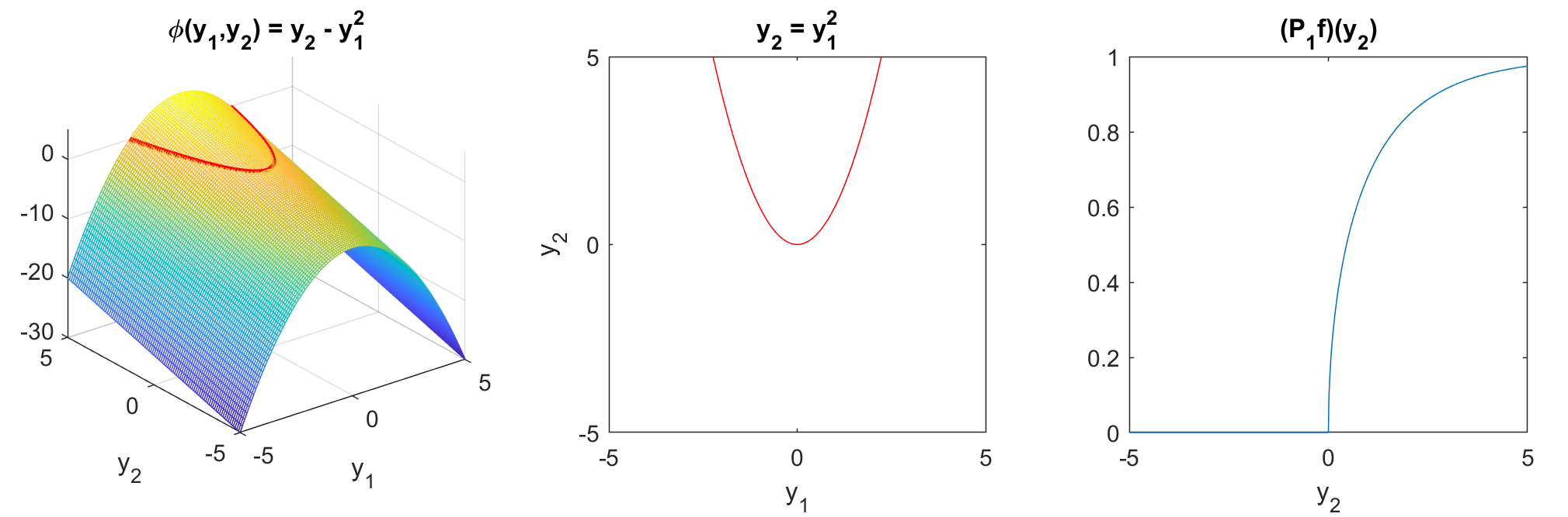
Figure 1: Illustrations for Example 1.

Example 1.

In this example we take

$$\phi(y_{1},y_{2})\,=\,y_{2}-y_{1}^{2},$$

see Figure 1 (left). The zero set of this function is the parabolic curve $y_{2}=y_{1}^{2}$, see Figure 1 (middle). The positivity set of $\phi$ (i.e., the set for which $f({\boldsymbol{y}})$ defined by (2) is non-zero) is the open region above the parabola.

If we take the special variable to be $y_{2}$ (i.e., if we take $j=2$) then the monotonicity condition (4) is satisfied, and the preintegration step is truly smoothing: specifically, we see that

$$(P_{2}f)(y_{1})\,=\,\int_{y_{1}^{2}}^{\infty}\rho(y_{2})\,{\mathrm{d}}y_{2}\,=\,1-\Phi(y_{1}^{2}),$$

where $\Phi(x):=\int_{-\infty}^{x}\rho(y)\,{\mathrm{d}}y$ is the standard normal cumulative distribution. Thus $(P_{2}f)(y_{1})$ is a smooth function for all $y_{1}\in{\mathbb{R}}$, and $I_{2}f$ is the integral of a smooth integrand over the real line,

$$I_{2}f\,=\,\int_{-\infty}^{\infty}(P_{2}f)(y_{1})\,\rho(y_{1})\,{\mathrm{d}}y_{1}\,=\,\int_{-\infty}^{\infty}\big{(}1-\Phi(y_{1}^{2})\big{)}\,\rho(y_{1})\,{\mathrm{d}}y_{1}.$$

If on the other hand we take the special variable to be $y_{1}$ (i.e., take $j=1$) then we have

$$(P_{1}f)(y_{2})\,=\,\begin{cases}0&\mbox{if }y_{2}\leq 0,\\ \displaystyle\int_{-\sqrt{y_{2}}}^{\sqrt{y_{2}}}\rho(y_{1})\,{\mathrm{d}}y_{1}\,=\,\Phi(\sqrt{y_{2}})-\Phi(-\sqrt{y_{2}})&\mbox{if }y_{2}>0.\end{cases}$$

The graph of $(P_{1}f)(y_{2})$, shown in Figure 1 (right), reveals that there is a singularity at $y_{2}=0$. To see the nature of the singularity, note that since $\rho(y_{1})=\rho(0)\exp(-y_{1}^{2}/2)=\rho(0)+{\mathcal{O}}(y_{1}^{2})$ as $y_{1}\to 0$, we can write

$$(P_{1}f)(y_{2})\,=\,\begin{cases}0&\mbox{if }y_{2}\leq 0,\\ \displaystyle\int_{-\sqrt{y_{2}}}^{\sqrt{y_{2}}}\rho(y_{1})\,{\mathrm{d}}y_{1}\,=\,2\sqrt{y_{2}}\,\rho(0)+{\mathcal{O}}\big{(}y_{2}^{3/2}\big{)}&\mbox{if }y_{2}>0.\end{cases}$$ (8)

Thus in this simple example $(P_{1}f)(y_{2})$ is not at all a smooth function of $y_{2}$, having a square-root singularity, and hence an infinite one-sided derivative, at $y_{2}=0$.

Figure 2: Illustrations for Example 2.

Example 2.

In this example we take

$$\phi(y_{1},y_{2})\,=\,y_{2}^{2}-y_{1}^{2}-1,$$

see Figure 2 (left). The zero set of $\phi$ is now the hyperbola $y_{2}^{2}=y_{1}^{2}+1$, see Figure 2 (middle), and the positivity set is the union of the open regions above and below the upper and lower branches respectively. Taking $j=1$, we see that monotonicity again fails, and that specifically

$$(P_{1}f)(y_{2})$$

$$\,=\,\begin{cases}0&\mbox{if }y_{2}\in[-1,1],\\ \displaystyle\int_{-\sqrt{y_{2}^{2}-1}}^{\sqrt{y_{2}^{2}-1}}\rho(y_{1})\,{\mathrm{d}}y_{1}\,=\,2\sqrt{y_{2}^{2}-1}\,\rho(0)+{\mathcal{O}}\big{(}(y_{2}^{2}-1)^{3/2}\big{)}&\mbox{if }|y_{2}|>1,\end{cases}$$

the graph of which is shown in Figure 2 (right). Again we see square-root singularities, this time two of them.

Example 3.

Here we take

$$\phi(y_{1},y_{2})\,=\,y_{2}^{2}-y_{1}^{2},$$

see Figure 3 (left). The level set is now the pair of lines $y_{2}=\pm y_{1}$, see Figure 3 (middle), and the positivity set is the open region above and below the crossed lines. This time $P_{1}f$ is given by

$$(P_{1}f)(y_{2})\,=\,\int_{-|y_{2}|}^{|y_{2}|}\rho(y_{1})\,{\mathrm{d}}y_{1}\,=\,2|y_{2}|\,\rho(0)+{\mathcal{O}}\big{(}|y_{2}|^{3}\big{)},$$

revealing in Figure 3 (right) a different kind of singularity (a simple discontinuity in the first derivative), but one still unfavorable for numerical integration.

Example 3 is rather special, in that the preintegration is performed on a line that touches a saddle at its critical point (the “flat” point” of the saddle). Example 4 below illustrates another situation, one that is in some ways similar to Example 1, but one perhaps less likely to be seen in practice.

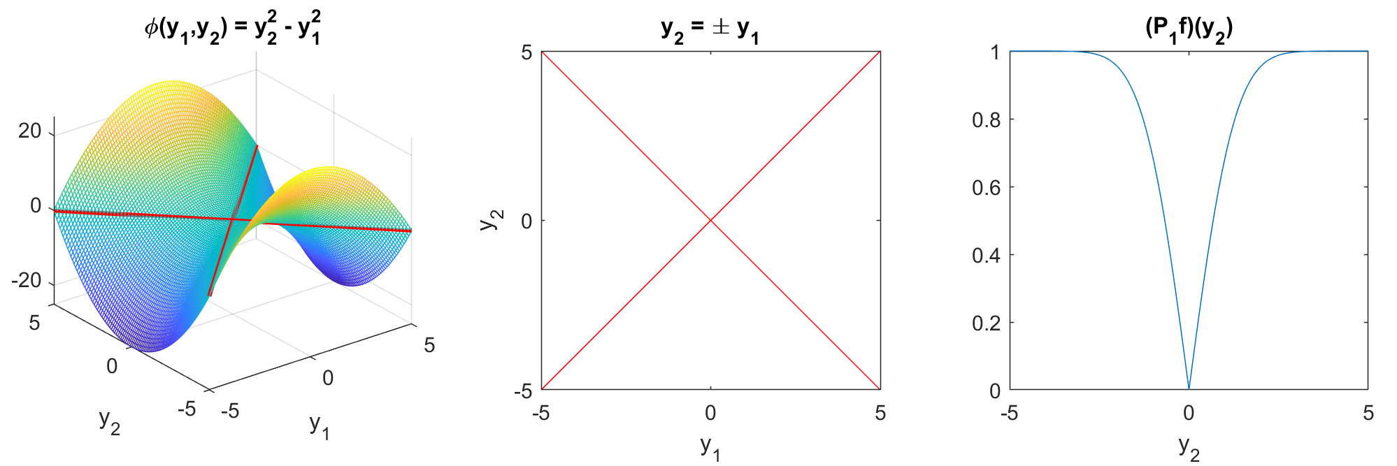
Figure 3: Illustrations for Example 3.

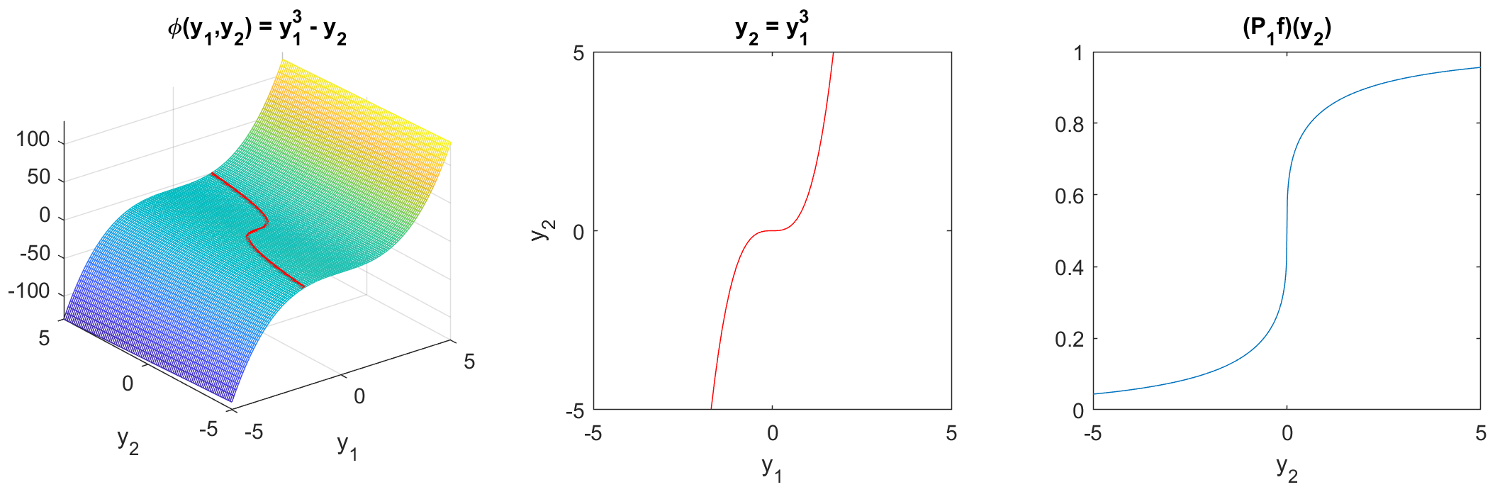
Figure 4: Illustrations for Example 4.

Example 4.

Here we consider

$$\phi(y_{1},y_{2})\,=\,y_{1}^{3}-y_{2},$$

see Figure 4 (left). The zero level set of $\phi$ is the graph of $y_{2}=y_{1}^{3}$, see Figure 4 (middle), and the positivity set is the unbounded domain to the right of the curve. We see that

$$(P_{1}f)(y_{2})\,=\,\int_{-\infty}^{y_{2}^{1/3}}\rho(y_{1})\,{\mathrm{d}}y_{1} \,=\,\int_{-\infty}^{0}\rho(y_{1})\,{\mathrm{d}}y_{1}+\int_{0}^{y_{2}^{1/3}}\rho(y_{1})\,{\mathrm{d}}y_{1}$$

$$\,=\,\frac{1}{2}+y_{2}^{1/3}\rho(0)+{\mathcal{O}}\big{(}|y_{2}|\big{)},$$

which holds regardless of the sign of $y_{2}$. The graph of $P_{1}f$ in Figure 4 (right) displays the cube-root singularity at $y_{2}=0$.

In each of the above examples we took $\theta(y_{1},y_{2})=1$. Other choices for $\theta$ are generally not interesting, as they do not affect the nature of the singularity. An exception is the choice $\theta(y_{1},y_{2})=\phi(y_{1},y_{2})$, which yields a kink rather than a jump because

$$\phi({\boldsymbol{y}})\,\mathop{\rm ind}(\phi({\boldsymbol{y}}))\,=\,\max(\phi({\boldsymbol{y}}),0),$$

and so leads to a weaker singularity. For example, for $f(y_{1},y_{2})=\max(\phi(y_{1},y_{2}),0)$ with $\phi$ as in Example 1, we obtain instead of (8)

$$(P_{1}f)(y_{2})\,=\,\begin{cases}0&\mbox{if }y_{2}\leq 0,\\ \displaystyle\int_{-\sqrt{y_{2}}}^{\sqrt{y_{2}}}(y_{2}-y_{1}^{2})\,\rho(y_{1})\,{\mathrm{d}}y_{1}\,=\,\frac{4}{3}\,y_{2}^{3/2}\,\rho(0)+{\mathcal{O}}\big{(}y_{2}^{5/2}\big{)}&\mbox{if }y_{2}>0.\end{cases}$$

With the recognition that kinks lead to less severe singularities than jumps, but located at the same places, from now on we shall for simplicity consider only the case $\theta({\boldsymbol{y}})=1$.

1.4 Outline of this paper

In Section 2 we study theoretically the smoothness of the preintegrated function, assuming that the original $d$-variate function is $f({\boldsymbol{y}})=\mathrm{ind}(\phi({\boldsymbol{y}})-t)$, with $\phi$ smooth but not monotone. We prove that the behavior seen in the above informative examples is typical. Section 3 contains a numerical experiment for a high-dimensional integrand that allows both monotone and non-monotone choices for the preintegrated variable. Section 4 gives brief conclusions.

2 Smoothness theorems in $d$ dimensions

In the general $d$-dimensional setting we take $\theta\equiv 1$, and use the general form (3) with arbitrary $t\in{\mathbb{R}}$. Thus now we consider

$$f({\boldsymbol{y}})\,:=\,f_{t}({\boldsymbol{y}})\,:=\,\mathop{\rm ind}\big{(}\phi({\boldsymbol{y}})-t\big{)},\quad{\boldsymbol{y}}\in{\mathbb{R}}^{d}.$$ (9)

A natural setting in which $t$ can take any value is in the computation of the (complementary) cumulative probability distribution of a random variable $X=\phi({\boldsymbol{y}})$, as in [6]. In the case of option pricing varying $t$ corresponds to varying the strike price.

For simplicity in this section we shall take the special preintegration variable to be $y_{1}$, so fixing $j=1$. The question is then, assuming that $\phi$ in (9) has smoothness at least $C^{2}({\mathbb{R}}^{d})$, whether or not $P_{1}f_{t}$ given by

$$(P_{1}f_{t})({\boldsymbol{y}}_{-1})\,\coloneqq\,\int_{-\infty}^{\infty}f_{t}(y_{1},{\boldsymbol{y}}_{-1})\,\rho(y_{1})\,{\mathrm{d}}y_{1}\,=\,\int_{-\infty}^{\infty}\mathop{\rm ind}\big{(}\phi({\boldsymbol{y}})-t\big{)}\,\rho(y_{1})\,{\mathrm{d}}y_{1}$$

is a smooth function of ${\boldsymbol{y}}_{-1}\in{\mathbb{R}}^{d-1}$.

To gain a first insight into the role of the parameter $t$ in (9), it is useful to observe that for the examples in Section 1.3 a variation in $t$ can change the position and even the nature of the singularity in $P_{1}f_{t}$, but does not necessarily eliminate the singularity. For a general $t\in{\mathbb{R}}$ and $\phi$ as in Example 1, we easily find that (8) is replaced by

$$(P_{1}f_{t})(y_{2})\,=\,\begin{cases}0&\mbox{if }y_{2}\leq t,\\ \displaystyle\int_{-\sqrt{y_{2}-t}}^{\sqrt{y_{2}-t}}\rho(y_{1})\,{\mathrm{d}}y_{1}&\mbox{if }y_{2}>t,\end{cases}$$

so that the graph of $P_{1}f_{t}$ is simply translated with the singularity now occurring at $y_{2}=t$ instead of $y_{2}=0$. The situation is the same for $\phi$ as in Example 4.

For $\phi$ as in Example 2, the choice $t=-1$ recovers Example 3, while for $t>-1$ we find

$$(P_{1}f_{t})(y_{2})\,=\,\begin{cases}0&\mbox{if }y_{2}\in[-\sqrt{1+t},\sqrt{1+t}\,],\\ \displaystyle\int_{-\sqrt{y_{2}^{2}-1-t}}^{\sqrt{y_{2}^{2}-1-t}}\rho(y_{1})\,{\mathrm{d}}y_{1}&\mbox{if }|y_{2}|>\sqrt{1+t}\,,\\ \end{cases}$$

thus in this case $(P_{1}f_{t})(y_{2})$ has square-root singularities at $y_{2}=\pm\sqrt{1+t}$. For the case $t<-1$ (which we leave to the reader) $P_{1}f_{t}$ has no singularity.

In [12] it was proved that $P_{1}f_{t}$ has the same smoothness as $\phi$, provided that

$$\frac{\partial\phi}{\partial y_{1}}({\boldsymbol{y}})>0\qquad\mbox{for all}\quad{\boldsymbol{y}}\in{\mathbb{R}}^{d},$$ (10)

together with some other technical conditions, see [12, Theorems 2 and 3].

Here we are interested in the situation when $\phi$ is not monotone increasing with respect to $y_{1}$ for all ${\boldsymbol{y}}_{-1}$. In that case (unless $\phi$ is always monotone decreasing) there is at least one point, say ${\boldsymbol{y}}^{*}=(y_{1}^{*},{\boldsymbol{y}}_{-1}^{*})\in{\mathbb{R}}^{d}$, at which $(\partial\phi/\partial y_{1})({\boldsymbol{y}}^{*})=0$. At such a point the gradient of $\phi$ is either zero or orthogonal to the $y_{1}$ axis. If $t$ in (9) has the value $t=\phi({\boldsymbol{y}}^{*})$ then there is generically a singularity of some kind in $P_{1}f_{t}$ at the point ${\boldsymbol{y}}^{*}_{-1}\in{\mathbb{R}}^{d-1}$. If $t\neq\phi({\boldsymbol{y}}^{*})$ then there is in general no singularity in $P_{1}f_{t}$ at the point ${\boldsymbol{y}}^{*}_{-1}\in{\mathbb{R}}^{d-1}$, but if $t$ is not constant then the risk of encountering a near-singularity is high.

The following theorem states a general result for the existence and the nature of the singularities induced in $P_{1}f_{t}$ in the common situation in which the second derivative of $\phi$ with respect to $y_{1}$ is non-zero at ${\boldsymbol{y}}={\boldsymbol{y}}^{*}$, the point at which the first derivative with respect to $y_{1}$ is zero.

Theorem 1.

Let $\phi\in C^{2}({\mathbb{R}}^{d})$, and assume that ${\boldsymbol{y}}^{*}=(y_{1}^{*},{\boldsymbol{y}}_{-1}^{*})\in{\mathbb{R}}^{d}$ is such that

$$\frac{\partial\phi}{\partial y_{1}}({\boldsymbol{y}}^{*})=0,\quad\frac{\partial^{2}\phi}{\partial y_{1}^{2}}({\boldsymbol{y}}^{*})\neq 0,\quad\mbox{and}\quad\nabla\phi({\boldsymbol{y}}^{*})\neq{\boldsymbol{0}}.$$ (11)

Define $t:=\phi({\boldsymbol{y}}^{*})$. Then $(P_{1}f_{t})({\boldsymbol{y}}_{-1})$ has a square-root singularity at ${\boldsymbol{y}}^{*}_{-1}\in{\mathbb{R}}^{d-1}$, similar to those in Examples 1 and 2, along any line in ${\mathbb{R}}^{d-1}$ through ${\boldsymbol{y}}^{*}_{-1}$ that is not orthogonal to $\nabla_{\!-1}\phi({\boldsymbol{y}}^{*}):=((\partial\phi/\partial y_{2})({\boldsymbol{y}}^{*}),(\partial\phi/\partial y_{3})({\boldsymbol{y}}^{*}),\ldots,(\partial\phi/\partial y_{d})({\boldsymbol{y}}^{*}))$.

Proof.

Since $\nabla\phi({\boldsymbol{y}}^{*})$ is not zero, and has no component in the direction of the $y_{1}$ axis, it follows that $\nabla\phi({\boldsymbol{y}}^{*})$ can be written as $(0,\nabla_{\!-1}\phi({\boldsymbol{y}}^{*}))$, where $\nabla_{\!-1}\phi({\boldsymbol{y}}^{*})=\nabla_{\!-1}\phi(y_{1}^{*},{\boldsymbol{y}}_{-1}^{*})$ is a non-zero vector in ${\mathbb{R}}^{d-1}$ orthogonal to the $y_{1}$ axis. Note that as ${\boldsymbol{y}}_{-1}$ changes in a neighborhood of ${\boldsymbol{y}}_{-1}^{*}$, the function $\phi(y_{1}^{*},{\boldsymbol{y}}_{-1})$ is increasing in the direction $\nabla_{\!-1}\phi({\boldsymbol{y}}^{*})$, and also in the direction of an arbitrary unit vector ${\boldsymbol{z}}$ in ${\mathbb{R}}^{d-1}$ that has a positive inner product with $\nabla_{\!-1}\phi({\boldsymbol{y}}^{*})$. Our aim now is to explore the nature of $P_{1}f_{t}$ on the line through ${\boldsymbol{y}}_{-1}^{*}\in{\mathbb{R}}^{d-1}$ that is parallel to any such unit vector ${\boldsymbol{z}}$.

For simplicity of presentation, and without loss of generality, we assume from now on that the unit vector ${\boldsymbol{z}}$ points in the direction of the positive $y_{2}$ axis. This allows us to write ${\boldsymbol{y}}=(y_{1},y_{2},y^{*}_{3},\ldots,y^{*}_{d})=:(y_{1},y_{2})$, temporarily ignoring all components other than the first two. In this $2$-dimensional setting we know that

$$\frac{\partial\phi}{\partial y_{1}}(y_{1}^{*},y_{2}^{*})=0,\quad\frac{\partial\phi}{\partial y_{2}}(y_{1}^{*},y_{2}^{*})>0,\quad\mbox{and}\quad\frac{\partial^{2}\phi}{\partial y_{1}^{2}}(y_{1}^{*},y_{2}^{*})\neq 0.$$

Since $(\partial\phi/\partial y_{2})(y_{1},y_{2})$ is continuous and positive at $(y_{1},y_{2})=(y_{1}^{*},y_{2}^{*})$, it follows that $(\partial\phi/\partial y_{2})(y_{1},y_{2})$ is positive on the rectangle $[y^{*}_{1}-\delta,y^{*}_{1}+\delta]\times[y^{*}_{2}-\delta,y^{*}_{2}+\delta]$ for sufficiently small $\delta>0$. Since $\phi(y_{1},y_{2})$ is increasing with respect to $y_{2}$ on this rectangle, it follows that for each $y_{1}\in[y^{*}_{1}-\delta,y^{*}_{1}+\delta]$ there is at most one value of $y_{2}$ such that $\phi(y_{1},y_{2})=t$, and further, that for $|y_{1}-y^{*}_{1}|$ sufficiently small there is exactly one value of $y_{2}$ such that $\phi(y_{1},y_{2})=t$. For that unique value we write $y_{2}=\zeta(y_{1})$, hence by construction we have $\phi(y_{1},\zeta(y_{1}))=t$, and $\zeta(y^{*}_{1})=y^{*}_{2}$.

From the implicit function theorem (or by implicit differentiation of $\phi(y_{1},\zeta(y_{1}))=t$ with respect to $y_{1}$) we obtain

$$\zeta^{\prime}(y_{1})\,=\,-\,\frac{(\partial\phi/\partial y_{1})(y_{1},\zeta(y_{1}))}{(\partial\phi/\partial y_{2})(y_{1},\zeta(y_{1}))},$$ (12)

in which the denominator is non-zero in a neighborhood of $y^{*}_{1}$. From this it follows that

$$\zeta^{\prime}(y^{*}_{1})\,=\,0.$$

Differentiating (12) using the product rule and the chain rule and then setting $y_{1}=y^{*}_{1}$ (so that several terms vanish), we obtain

$$\zeta^{\prime\prime}(y^{*}_{1})\,=\,-\,\frac{(\partial^{2}\phi/\partial y_{1}^{2})(y^{*}_{1},y^{*}_{2})}{(\partial\phi/\partial y_{2})(y^{*}_{1},y^{*}_{2})},$$

which by assumption is non-zero. Below we assume that $(\partial^{2}\phi/\partial y_{1}^{2})(y^{*}_{1},y^{*}_{2})<0$, from which it follows that $\zeta^{\prime\prime}(y^{*}_{1})$ is positive; the case $(\partial^{2}\phi/\partial y_{1}^{2})(y^{*}_{1},y^{*}_{2})>0$ is similar. Taylor’s theorem with remainder gives

$$\zeta(y_{1}) \,=\,\zeta(y^{*}_{1})+\tfrac{1}{2}(y_{1}-y^{*}_{1})^{2}\,\zeta^{\prime\prime}(y^{*}_{1})\,(1+o(1))$$

$$\,=\,y^{*}_{2}+\tfrac{1}{2}(y_{1}-y^{*}_{1})^{2}\,\zeta^{\prime\prime}(y^{*}_{1})\,(1+o(1)),$$ (13)

where $o(1)\to 0$ as $|y_{1}-y^{*}_{1}|\to 0$, thus $\zeta(y_{1})$ is a convex function in a neighborhood of $y^{*}_{1}$.

Given $y_{2}$ in a neighborhood of $y^{*}_{2}$, our task now is to evaluate the contribution to the integral

$$(P_{1}f_{t})(y_{2})\,=\,\int_{-\infty}^{\infty}\mathop{\rm ind}\big{(}\phi(y_{1},y_{2})-t\big{)}\rho(y_{1})\,{\mathrm{d}}y_{1}$$

from a neighborhood of $y^{*}_{1}$. Thus we need to find the set of $y_{1}$ values in a neighborhood of $y^{*}_{1}$ for which $\phi(y_{1},y_{2})>t$. Because of (2), the set is either empty, or is the open interval with extreme points given by the solutions of $\zeta(y_{1})=y_{2}$, i.e.,

$$y^{*}_{2}+\tfrac{1}{2}(y_{1}-y^{*}_{1})^{2}\,\zeta^{\prime\prime}(y^{*}_{1})\,(1+o(1))\,=\,y_{2},$$

implying

$$(y_{1}-y^{*}_{1})^{2}\,=\,\frac{2(y_{2}-y^{*}_{2})}{\zeta^{\prime\prime}(y^{*}_{1})\,(1+o(1))}\,=\,\frac{2(y_{2}-y^{*}_{2})}{\zeta^{\prime\prime}(y^{*}_{1})}(1+o(1)).$$

There is no solution for $y_{2}<y^{*}_{2}$, while for $y_{2}>y^{*}_{2}$ the solutions are

$$y_{1}\,=\,y^{*}_{1}\pm c\sqrt{y_{2}-y^{*}_{2}}\,(1+o(1)),$$

with $c:=\sqrt{2/\zeta^{\prime\prime}(y^{*}_{1})}$. Thus the contribution to $P_{1}f_{t}(y_{2})$ from the neighborhood of $y^{*}_{2}$ is zero for $y_{2}<y^{*}_{2}$, and for $y_{2}>y^{*}_{2}$ is

$$\int_{y^{*}_{1}-c\sqrt{y_{2}-y^{*}_{2}}\,(1+o(1))}^{y^{*}_{1}+c\sqrt{y_{2}-y^{*}_{2}}\,(1+o(1))}\rho(y_{1})\,{\mathrm{d}}y_{1}\,=\,2c\sqrt{y_{2}-y^{*}_{2}}\,\rho(y^{*}_{1})\,(1+o(1)).$$

Thus there is a singularity in $P_{1}f_{t}$ of exactly the same character as that in Examples 1 and 2. ∎

Remark 1.

We now return to consider the examples in Section 1.3 in the context of Theorem 1.

• For $\phi$ as in Example 1, we have $(\partial\phi/\partial y_{1})(y_{1},y_{2})=-2y_{1}$, $(\partial^{2}\phi/\partial y_{1}^{2})(y_{1},y_{2})=-2\neq 0$, and $\nabla\phi(y_{1},y_{2})=(-2y_{1},1)\neq(0,0)$. Thus (11) holds, e.g., with ${\boldsymbol{y}}^{*}=(0,0)$ and $t=\phi({\boldsymbol{y}}^{*})=0$, and $P_{1}f_{t}$ indeed displays the predicted square-root singularity at $y_{2}=0$, see Figure 1.

• For $\phi$ as in Example 2, we have $(\partial\phi/\partial y_{1})(y_{1},y_{2})=-2y_{1}$, $(\partial^{2}\phi/\partial y_{1}^{2})(y_{1},y_{2})=-2\neq 0$, and $\nabla\phi(y_{1},y_{2})=(-2y_{1},2y_{2})$. Thus (11) holds, e.g., with ${\boldsymbol{y}}^{*}=(0,\pm 1)$ and $t=\phi({\boldsymbol{y}}^{*})=0$, and $P_{1}f_{t}$ indeed shows the predicted square-root singularities at $y_{2}=\pm 1$, see Figure 2.

• For $\phi$ as in Example 3, we have the same derivative expressions as in Example 2. Thus (11) holds, e.g., again with ${\boldsymbol{y}}^{*}=(0,\pm 1)$, but now $t=\phi({\boldsymbol{y}}^{*})=1$, and we effectively recover Example 2 with square-root singularities for $P_{1}f_{t}$ at $y_{2}=\pm 1$. However, if we consider instead the point ${\boldsymbol{y}}^{\dagger}=(0,0)$ and $t=\phi({\boldsymbol{y}}^{\dagger})=0$, as in Figure 3, then we have $\nabla\phi({\boldsymbol{y}}^{\dagger})=0$ so the non-vanishing gradient condition in (11) fails and Theorem 1 does not apply at this point ${\boldsymbol{y}}^{\dagger}$. In this case we actually observe an absolute-value singularity for $P_{1}f_{t}$ at $y_{2}=0$ rather than a square-root singularity.

• For $\phi$ as in Example 4, we have $(\partial\phi/\partial y_{1})(y_{1},y_{2})=3y_{1}^{2}$, $(\partial^{2}\phi/\partial y_{1}^{2})(y_{1},y_{2})=6y_{1}$, and $\nabla\phi(y_{1},y_{2})=(3y_{1}^{2},-1)\neq(0,0)$. It is impossible to satisfy both the first and second conditions in (11) so Theorem 1 does not apply anywhere. In particular, at the point ${\boldsymbol{y}}^{\dagger}=(0,0)$ and $t=\phi({\boldsymbol{y}}^{\dagger})=0$, as in Figure 4, we have $(\partial^{2}\phi/\partial y_{1}^{2})({\boldsymbol{y}}^{\dagger})=0$, and in consequence (given that the third derivative does not vanish) $P_{1}f_{t}$ has a cube-root singularity at $y_{2}=0$ rather than a square-root singularity.

From Theorem 1 one might suspect, because $t$ in the theorem has the particular value $t=\phi({\boldsymbol{y}}^{*})$, that singularities of this kind are rare. However, in the following theorem we show that values of $t\in{\mathbb{R}}$ at which singularities occur in $P_{1}f_{t}$ are generally not isolated. This is essentially because points at which $(\partial\phi/\partial y_{1})({\boldsymbol{y}})=0$ are themselves generally not isolated.

Theorem 2.

Let $\phi\in C^{2}({\mathbb{R}}^{d})$, and assume that ${\boldsymbol{y}}^{*}\in{\mathbb{R}}^{d}$ is such that

$$\frac{\partial\phi}{\partial y_{1}}({\boldsymbol{y}}^{*})=0,\quad\nabla\phi({\boldsymbol{y}}^{*})\neq{\boldsymbol{0}},\quad\mbox{and}\quad\nabla\frac{\partial\phi}{\partial y_{1}}({\boldsymbol{y}}^{*})\neq{\boldsymbol{0}},$$ (14)

with $\nabla\phi({\boldsymbol{y}}^{*})$ not parallel to $\nabla(\partial\phi/\partial y_{1})({\boldsymbol{y}}^{*})$. Then for any $t$ in some open interval containing $\phi({\boldsymbol{y}}^{*})$ there exists a point ${\boldsymbol{y}}^{(t)}\in{\mathbb{R}}^{d}$ in a neighborhood of ${\boldsymbol{y}}^{*}$ at which

$$\phi({\boldsymbol{y}}^{(t)})=t,\quad\frac{\partial\phi}{\partial y_{1}}({\boldsymbol{y}}^{(t)})=0,\quad\mbox{and}\quad\nabla\phi({\boldsymbol{y}}^{(t)})\neq{\boldsymbol{0}}.$$ (15)

Moreover, if we assume also that $(\partial^{2}\phi/\partial y_{1}^{2})({\boldsymbol{y}}^{*})\neq 0$, then the preintegrated quantity $(P_{1}f_{t})({\boldsymbol{y}}_{-1})$ has a square-root singularity at ${\boldsymbol{y}}^{(t)}_{-1}\in{\mathbb{R}}^{d-1}$ along any line in ${\mathbb{R}}^{d-1}$ through ${\boldsymbol{y}}^{(t)}_{-1}$ that is not orthogonal to $\nabla\phi({\boldsymbol{y}}^{(t)})$.

Proof.

It is convenient to define $\psi({\boldsymbol{y}}):=(\partial\phi/\partial y_{1})({\boldsymbol{y}})$, which by assumption is a real-valued $C^{1}(\mathbb{R}^{d})$ function that satisfies

$$\psi({\boldsymbol{y}}^{*})=0\quad\mbox{and}\quad\nabla\psi({\boldsymbol{y}}^{*})\neq{\boldsymbol{0}}.$$

We need to show that for $t$ in some open interval containing $\phi({\boldsymbol{y}}^{*})$ there exists ${\boldsymbol{y}}^{(t)}\in\mathbb{R}^{d}$ in a neighborhood of ${\boldsymbol{y}}^{*}$ at which

$$\phi({\boldsymbol{y}}^{(t)})=t,\quad\psi({\boldsymbol{y}}^{(t)})=0,\quad\mbox{and}\quad\nabla\phi({\boldsymbol{y}}^{(t)})\neq{\boldsymbol{0}}.$$

Clearly, we can confine our search for ${\boldsymbol{y}}^{(t)}$ to the zero level set of $\psi$, that is, to the solutions of

$$\psi({\boldsymbol{y}})=0,\quad{\boldsymbol{y}}\in\mathbb{R}^{d}.$$

Since $\nabla\psi({\boldsymbol{y}})$ is continuous and non-zero in a neighborhood of ${\boldsymbol{y}}^{*}$, the zero level set of $\psi$ is a manifold of dimension $d-1$ near ${\boldsymbol{y}}^{*}$, whose tangent hyperplane at ${\boldsymbol{y}}^{*}$ is orthogonal to $\nabla\psi({\boldsymbol{y}}^{*})$, see, e.g., [16, Chapter 5]. On this hyperplane there is a search direction starting from ${\boldsymbol{y}}^{*}$ for which $\phi({\boldsymbol{y}})$ has a maximal rate of increase, namely the direction of the orthogonal projection of $\nabla\phi({\boldsymbol{y}}^{*})$ onto the tangent hyperplane, noting that this is a non-zero vector because $\nabla\phi({\boldsymbol{y}}^{*})$ is not parallel to $\nabla\psi({\boldsymbol{y}}^{*})$. Setting out from the point ${\boldsymbol{y}}^{*}$ in the direction of positive gradient, the value of $\phi$ is strictly increasing in a sufficiently small neighborhood of ${\boldsymbol{y}}^{*}$, while in the direction of negative gradient it is strictly decreasing. Thus searching on the manifold for a ${\boldsymbol{y}}^{(t)}$ such that $\phi({\boldsymbol{y}}^{(t)})=t$ will be successful in one of these directions for $t$ in a sufficiently small open interval containing $\phi({\boldsymbol{y}}^{*})$.

Under the additional assumption that $(\partial^{2}\phi/\partial y_{1}^{2})({\boldsymbol{y}}^{*})\neq 0$, all the conditions of Theorem 1 are satisfied with ${\boldsymbol{y}}^{*}$ replaced by ${\boldsymbol{y}}^{(t)}$, noting that because $\phi\in C^{2}(\mathbb{R}^{d})$ the second derivative is also non-zero in a sufficiently small neighborhood of ${\boldsymbol{y}}^{*}$. This completes the proof. ∎

Remark 2.

We now show that for $\phi$ as in Examples 1–4 the singularities in $P_{1}f_{t}$, with $f_{t}$ as in (9), are not isolated and furthermore, we give the exact regions in which the singularities exist.

• For $\phi$ as in Example 1 we may choose ${\boldsymbol{y}}^{*}=(0,0)$, as in Remark 1. Indeed, the gradient of the first derivative with respect to $y_{1}$ is $\nabla(\partial\phi/\partial y_{1})(y_{1},y_{2})=(-2,0)$, which is not parallel to $\nabla\phi(y_{1},y_{2})=(-2y_{1},1)$ for all $(y_{1},y_{2})\in{\mathbb{R}}^{2}$. It follows that (14) holds, e.g., at ${\boldsymbol{y}}^{*}=(0,0)$. Hence Theorem 2 implies that for $t$ in some interval around $\phi({\boldsymbol{y}}^{*})=0$ there is ${\boldsymbol{y}}^{(t)}=(y_{1}^{(t)},y_{2}^{(t)})$ in a neighborhood of ${\boldsymbol{y}}^{*}=(0,0)$ such that $\phi({\boldsymbol{y}}^{(t)})=t$ and (15) holds. In particular, there is still a square-root singularity in $(P_{1}f_{t})(y_{2})$ at $y_{2}=y_{2}^{(t)}$. We confirm that this is indeed the case by taking ${\boldsymbol{y}}^{(t)}=(0,t)$ and by observing that, as is easily verified, $(P_{1}f_{t})(y_{2})$ has a square-root singularity at $y_{2}=t$ for all real numbers $t$. This singularity in $P_{1}f_{t}$ is similar to the singularity depicted in Figure 1, but translated by $t$.

• For $\phi$ as in Example 3 we can consider ${\boldsymbol{y}}^{*}=(0,\pm 1)$ as in Remark 1. The gradient of the first derivative with respect to $y_{1}$ is $\nabla(\partial\phi/\partial y_{1})(y_{1},y_{2})=(-2,0)$, which is not parallel to $\nabla\phi(y_{1},y_{2})=(-2y_{1},2y_{2})$ for all $(y_{1},y_{2})\in{\mathbb{R}}^{2}$ with $y_{2}\neq 0$. Thus (14) holds, e.g., at ${\boldsymbol{y}}^{*}=(0,\pm 1)$. Theorem 2 implies that for $t$ in some interval around $\phi({\boldsymbol{y}}^{*})=1$ there is a point ${\boldsymbol{y}}^{(t)}$ in a neighborhood of ${\boldsymbol{y}}^{*}=(0,\pm 1)$ such that $\phi({\boldsymbol{y}}^{(t)})=t$, (15) holds, and $(P_{1}f_{t})(y_{2})$ has a square-root singularity at $y_{2}=y_{2}^{(t)}$. Indeed, for any real number $t>0$, taking ${\boldsymbol{y}}^{(t)}=(0,\pm\sqrt{t})$ gives $\phi({\boldsymbol{y}}^{(t)})=t$, and it can easily be verified that $(P_{1}f_{t})(y_{2})$ has two square-root singularities at $y_{2}=\pm\sqrt{t}$. In this case the behavior of $P_{1}f_{t}$ is similar to Figure 2, with the location of the singularities now depending on $t$.

• Since $\phi$ from Example 2 is simply a translation of Example 3 by $-1$, similar singularities exist for that case for $t>-1$.

• For $\phi$ as in Example 4 the condition (14) never holds, since $\nabla(\partial\phi/\partial y_{1})(y_{1},y_{2})=(0,0)$ whenever $(\partial\phi/\partial y_{1})(y_{1},y_{2})=0$. So no conclusion can be drawn from Theorem 2 in this case. It is no contradiction that, as is easily seen, there is a singularity (of cube-root character) in $(P_{1}f_{t})(y_{2})$ at $y_{2}=t$ for every real number $t$.

3 A high-dimensional example

Motivated by applications in computational finance, for a high-dimensional example we consider the problem of approximating the fair price for a digital Asian option, a problem that can be formulated as an integral as in (1) with a discontinuous integrand of the form (9). When monotonicity holds, it was shown in [12] that preintegration not only has theoretical smoothing benefits, but also that when followed by a QMC rule to compute the $(d-1)$-dimensional integral the computational experience can be excellent. On the other hand that paper provided no insight as to what happens, either theoretically or numerically, when monotonicity fails. In this section, in contrast, we will deliberately apply preintegration using a chosen variable for which the monotonicity condition fails. We will demonstrate the resulting lack of smoothness, using the theoretical results from the previous section, and show that the performance of the subsequent QMC rule can degrade when the preintegration variable lacks the monotonicity property.

For a given strike price $K$, the payoff for a digital Asian call option is given by

$$\mathrm{payoff}\,=\,\mathop{\rm ind}(\phi-K),$$

where $\phi$ is the average price of the underlying stock over the time period. Under the Black–Scholes model the time-discretised average is given by

$$\phi({\boldsymbol{y}})\,=\,\frac{S_{0}}{d}\sum_{k=1}^{d}\exp\bigg{(}(r-\tfrac{1}{2}\sigma^{2})\frac{kT}{d}+\sigma{\boldsymbol{A}}_{k}{\boldsymbol{y}}\bigg{)},$$ (16)

where ${\boldsymbol{y}}=(y_{k})_{k=1}^{d}$ is a vector of i.i.d. standard normal random variables, $S_{0}$ is the initial stock price, $T$ is the final time, $r$ is the risk-free interest rate, $\sigma$ is the volatility and $d$ is the number of timesteps, which is also the dimension of the problem. Note that in (16) we have already made a change of variables to write the problem in terms of standard normal random variables, by factorising the covariance matrix of the Brownian motion increments as $\Sigma=AA^{\top}$, where the entries of the covariance matrix are $\Sigma_{k,\ell}=\min(k,\ell)\times T/d$. Then in (16), ${\boldsymbol{A}}_{k}$ denotes the $k$th row of this matrix factor.

The fair price of the option is then given by the discounted expected payoff

$$e^{-rT}\,{\mathbb{E}}[\mathrm{payoff}]\,=\,e^{-rT}\int_{{\mathbb{R}}^{d}}\mathop{\rm ind}(\phi({\boldsymbol{y}})-K)\rho_{d}({\boldsymbol{y}})\,\mathrm{d}{\boldsymbol{y}}\,.$$ (17)

Letting $f({\boldsymbol{y}})=\mathop{\rm ind}(\phi({\boldsymbol{y}})-K)$, this example clearly fits into the framework (9) where $\phi$ is the average stock price (16), $t$ is the strike price $K$ and each $\rho$ is a standard normal density.

There are three popular methods for factorising the covariance matrix: the standard construction (which uses the Cholesky factorisation), Brownian bridge, and principal components or PCA, see, e.g., [7] for further details. In the first two cases all components of the matrix $A$ are positive, in which case it is easily seen by studying the derivative of (16) with respect to $y_{j}$ for some $j=1,\ldots,d$,

$$\frac{\partial\phi}{\partial y_{j}}({\boldsymbol{y}})\,=\,\frac{S_{0}}{d}\sum_{k=1}^{d}\sigma A_{k,j}\exp\bigg{(}(r-\tfrac{1}{2}\sigma^{2})\frac{kT}{d}+\sigma{\boldsymbol{A}}_{k}{\boldsymbol{y}}\bigg{)},$$

that $\phi$ is monotone increasing with respect to $y_{j}$ no matter which $j$ is chosen.

In contrast, for the PCA construction, which we consider below, the situation is very different, in that there is only one choice of $j$ for which $\phi$ is monotone with respect to $y_{j}$. This is because with PCA the factorisation of $\Sigma$ employs its eigendecomposition, with the $j$th column of $A$ being a (scaled) eigenvector corresponding to the $j$th eigenvalue labeled in decreasing order. Since the covariance matrix $\Sigma$ is positive definite the eigenvector corresponding to the largest eigenvalue has all components positive, thus for $j=1$ monotonicity of $\phi$ is achieved. On the other hand, every eigenvector other than the first is orthogonal to the first, and therefore must have components of both signs. Given that

$$A_{k,j}>0\implies\exp(A_{k,j}y_{j})\to\begin{cases}+\infty&\mbox{as }y_{j}\to+\infty,\\ 0&\mbox{as }y_{j}\to-\infty,\end{cases}$$

$$A_{k,j}<0\implies\exp(A_{k,j}y_{j})\to\begin{cases}0&\mbox{as }y_{j}\to+\infty,\\ +\infty&\mbox{as }y_{j}\to-\infty,\end{cases}$$

it follows that for $j\neq 1$ there is at least one term in the sum over $k$ in (16) that approaches $+\infty$ as $y_{j}\to+\infty$ and at least one other term that approaches $+\infty$ as $y_{j}\to-\infty$. Given that all terms in the sum over $k$ in (16) are positive, it follows that for the PCA case and $j\neq 1$, $\phi$ must approach $+\infty$ as $y_{j}\to\pm\infty$, so is definitely not monotone. Moreover, with respect to each variable $y_{j}$ the function $\phi$ is strictly convex, since

$$\frac{\partial^{2}\phi}{\partial y_{j}^{2}}({\boldsymbol{y}})\,=\,\frac{S_{0}}{d}\sum_{k=1}^{d}(\sigma A_{k,j})^{2}\exp\bigg{(}(r-\tfrac{1}{2}\sigma^{2})\frac{kT}{d}+\sigma{\boldsymbol{A}}_{k}{\boldsymbol{y}}\bigg{)}\,>\,0\quad\text{for all }{\boldsymbol{y}}\in{\mathbb{R}}^{d}.$$

For definiteness, in the following discussion we denote by $y_{2}$ the preintegration variable for which monotonicity fails, and denote the other variables by ${\boldsymbol{y}}_{-2}=(y_{1},y_{3},\ldots,y_{d})$. We now use the results from the previous section to determine the smoothness, or rather the lack thereof, of $P_{2}f$ when $f({\boldsymbol{y}})=\mathop{\rm ind}(\phi({\boldsymbol{y}})-K)$. To do this we will use Theorem 1 and Theorem 2, where with a slight abuse of notation we replace $y_{1}$ by $y_{2}$ as our special preintegration variable.

First, note that we have already established that $\phi$ is not monotone with respect to $y_{2}$, and since $\phi$ is strictly convex with respect to $y_{2}$, for a given ${\boldsymbol{y}}_{-2}$ there exists a unique $y_{2}^{*}\in{\mathbb{R}}$ such that $(\partial\phi/\partial y_{2})(y_{2}^{*},{\boldsymbol{y}}_{-2})=0$. Since $\phi$ is strictly increasing with respect to $y_{1}$, it follows that $\nabla\phi(y_{2}^{*},{\boldsymbol{y}}_{-2})\neq{\boldsymbol{0}}$. Furthermore, since $(\partial^{2}\phi/\partial y_{2}^{2})(y_{2}^{*},{\boldsymbol{y}}_{-2})>0$, Theorem 1 implies that for $K=\phi(y_{2}^{*},{\boldsymbol{y}}_{-2})$ the preintegrated function $P_{2}f$ has a square-root singularity along any line not orthogonal to $\nabla_{\!-2}\phi(y_{2}^{*},{\boldsymbol{y}}_{-2})$, with $\nabla_{\!-2}$ defined analogously to $\nabla_{\!-1}$ in Theorem 1.

Furthermore, Theorem 2 implies that this singularity is not isolated. To apply Theorem 2 we note that we have already established the first two conditions in (14) (recall again that we now take $y_{2}$ as the preintegration variable). We also have $(\partial^{2}\phi/\partial y_{2}^{2})(y_{2}^{*},{\boldsymbol{y}}_{-2})>0$, which implies $\nabla(\partial\phi/\partial y_{2})(y_{2}^{*},{\boldsymbol{y}}_{-2})\neq{\boldsymbol{0}}$. Moreover, we know that $\nabla(\partial\phi/\partial y_{2})(y_{2}^{*},{\boldsymbol{y}}_{-2})$ and $\nabla\phi(y_{2}^{*},{\boldsymbol{y}}_{-2})$ are not parallel, since the former has a positive second component while the latter has a zero second component.

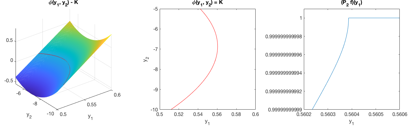
Figure 5: Illustrations for digital Asian option in two dimensions.

To visualise this singularity, in Figure 5 we provide an illustration of the option in two dimensions. (Note that we consider $d=2$ here for visualisation purposes only; we have shown already that the singularity exists for any choice of $d>1$. Later we present numerical results for $d=256$.) Figure 5 gives a contour plot of $\phi(y_{1},y_{2})-K$ (left), the zero level set of $\phi(y_{1},y_{2})=K$ (middle) and then the graph of $P_{2}f$ (right). As expected, we can clearly see that $P_{2}f$ has a singularity that is of square-root nature.

To perform the preintegration step $P_{2}f$ in practice, note that since $\phi$ is strictly convex with respect to $y_{2}$ for each ${\boldsymbol{y}}_{-2}\in{\mathbb{R}}^{d-1}$ there is a single turning point $y_{2}^{*}\in{\mathbb{R}}$ for which $(\partial\phi/\partial y_{2})(y_{2}^{*},{\boldsymbol{y}}_{-2})=0$ and $\phi(y_{2}^{*},{\boldsymbol{y}}_{-2})$ is a global minimum. It follows that there are at most two distinct points, $\xi_{a}({\boldsymbol{y}}_{-2})\leq\xi_{b}({\boldsymbol{y}}_{-2})$, such that

$$\phi(\xi_{a}({\boldsymbol{y}}_{-2}),{\boldsymbol{y}}_{-2})\,=\,K\,=\,\phi(\xi_{b}({\boldsymbol{y}}_{-2}),{\boldsymbol{y}}_{-2})\,.$$

Preintegration with respect to $y_{2}$ then simplifies to

$$(P_{2}f)({\boldsymbol{y}}_{-2})\, =\,\int_{-\infty}^{\infty}\mathop{\rm ind}(\phi(y_{2},{\boldsymbol{y}}_{-2})-K)\,\rho(y_{2})\,\mathrm{d}y_{2}$$

$$=\,\begin{cases}1&\text{if }\phi(y_{2}^{*},{\boldsymbol{y}}_{-2})\geq K,\\[5.69054pt] \displaystyle\int_{-\infty}^{\xi_{a}({\boldsymbol{y}}_{-2})}\rho(y_{2})\,\mathrm{d}y_{2}+\int_{\xi_{b}({\boldsymbol{y}}_{-2})}^{\infty}\rho(y_{2})\,\mathrm{d}y_{2}&\text{otherwise},\end{cases}$$

$$=\,\begin{cases}1&\text{if }\phi(y_{2}^{*},{\boldsymbol{y}}_{-2})\geq K,\\[5.69054pt] \Phi(\xi_{a}({\boldsymbol{y}}_{-2}))+1-\Phi(\xi_{b}({\boldsymbol{y}}_{-2}))\hskip 42.67912pt&\text{otherwise}.\end{cases}$$

In practice, for each ${\boldsymbol{y}}_{-2}\in{\mathbb{R}}^{d-1}$ the turning point $y_{2}^{*}$ and the points of discontinuity $\xi_{a}({\boldsymbol{y}}_{-2})$ and $\xi_{b}({\boldsymbol{y}}_{-2})$ are computed numerically, e.g., by Newton’s method.

We now look at how this lack of smoothness affects the performance of using a numerical preintegration method to approximate the fair price for the digital Asian option in $d=256$ dimensions. Explicitly, we approximate the integral in (17) by applying a $(d-1)$-dimensional QMC rule to $P_{2}f$. As a comparison, we also present results for approximating the integral in (17) by applying the same QMC rule to $P_{1}f$. Recall that $\phi$ is monotone in dimension $1$ and furthermore, it was shown in [12] that $P_{1}f$ is smooth.

For the QMC rule we use a randomly shifted lattice rule based on the generating vector lattice-32001-1024-1048576.3600 from [14] using $N=2^{10},2^{11},\ldots,2^{19}$ points with $R=16$ random shifts. The parameters for the option are $S_{0}=\$100$, $K=\$110$, $T=1$, $d=256$ timesteps, $r=0.1$ and $\sigma=0.1$. We also performed a standard Monte Carlo approximation using $R\times N$ points and a plain (without preintegration) QMC approximation using the same generating vector.

In Figure 6, we plot the convergence of the standard error, which we estimate by the sample standard error over the different random shifts, in terms of the total number of function evaluations $R\times N$. We can clearly see that preintegration with respect to $y_{2}$ produces less accurate results compared to preintegration with respect to $y_{1}$, with errors that are up to an order of magnitude larger for the higher values of $N$. We also note that to achieve a given error, say $10^{-4}$, the number of points needs to be increased tenfold. Furthermore, we observe that the empirical convergence rate for preintegration with respect to $y_{2}$ is $N^{-0.9}$, which is sightly worse than the rate of $N^{-0.98}$ for preintegration with respect to $y_{1}$. Hence, when the monotonicity condition fails, not only does the theory for QMC fail due to the presence of a singularity, but we also observe worse results in practice and somewhat slower convergence.

We also plot the error of standard Monte Carlo and QMC approximations, which behave as expected and are both significantly outperformed by the two preintegration methods.

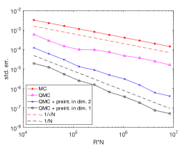
Figure 6: Convergence in $N$ for different approximations of the fair price for a digital Asian option.

4 Conclusion

If the monotonicity property (10) fails and $f=f_{t}$ is defined by (9) then we have seen that generically there is a singularity in $P_{1}f$ for some values of $t$, and under known conditions this is true even for values of $t$ in an interval.

It should also be noted that implementation of preintegration is more difficult if monotonicity fails, since instead of a single integral from $\xi({\boldsymbol{y}}_{-1})$ to $\infty$, as in (7), there will in general be additional finite or infinite intervals to integrate over, all of whose end points must be discovered by the user for each required value of ${\boldsymbol{y}}_{-1}$.

To explore the consequences of a lack of monotonicity empirically, we carried out in Section 3 a $256$-dimensional calculation of pricing a digital Asian option, first by preintegrating with respect to a variable known to lack the monotonicity property, and then with a variable where the property holds, with the result that both accuracy and rate of convergence were observed to be degraded when monotonicity fails.

There is an additional problem of preintegrating with respect to a variable for which the monotonicity fails, namely that because of the proven lack of smoothness, the resulting preintegrated function no longer belongs to the space of $(d-1)$-variate functions of dominating mixed smoothness of order one, and as a consequence there is at present no theoretical support for our use of QMC integration for this $(d-1)$-dimensional integral.

The practical significance of this paper is that effective use of preintegration is greatly enhanced by the preliminary identification of a special variable for which the monotonicity property is known to hold. The paper does not offer guidance on the choice of variable if there is more than one such variable; in such cases it may be natural to choose the variable for which preintegration leads to the greatest reduction in variance.

References

- [1] N. Achtsis, R. Cools, and D. Nuyens, Conditional sampling for barrier option pricing under the LT method, SIAM J. Financial Math. 4 (2013), 327–352.
- [2] N. Achtsis, R. Cools, and D. Nuyens, Conditional sampling for barrier option pricing under the Heston model, in: J. Dick, F.Y. Kuo, G.W. Peters, I.H. Sloan (eds.), Monte Carlo and Quasi-Monte Carlo Methods 2012, pp. 253–269, Springer-Verlag, Berlin/Heidelberg (2013).
- [3] C. Bayer, M. Siebenmorgen, and R. Tempone, Smoothing the payoff for efficient computation of Basket option prices, Quant. Finance 18 (2018), 491–505.
- [4] H. Bungartz and M. Griebel, Sparse grids, Acta Numer. 13 (2004), 147–269.
- [5] J. Dick, F. Y. Kuo, and I. H. Sloan, High dimensional integration – the quasi-Monte Carlo way, Acta Numer. 22 (2013), 133–288.
- [6] A. D. Gilbert, F. Y. Kuo, and I. H. Sloan, Approximating distribution functions and densities using quasi-Monte Carlo methods after smoothing by preintegration, arXiv:2112.10308, (2021).
- [7] P. Glasserman, Monte Carlo Methods in Financial Engineering, Springer-Verlag, Berlin-Heidelberg, (2003).
- [8] P. Glasserman and J. Staum, Conditioning on one-step survival for barrier option simulations, Oper. Res., 49 (2001), 923–937.
- [9] M. Griebel, F. Y. Kuo, and I. H. Sloan, The smoothing effect of the ANOVA decomposition, J. Complexity 26 (2010), 523–551.
- [10] M. Griebel, F. Y. Kuo, and I. H. Sloan, The smoothing effect of integration in and the ANOVA decomposition, Math. Comp. 82 (2013), 383–400.
- [11] M. Griebel, F. Y. Kuo, and I. H. Sloan, Note on “the smoothing effect of integration in and the ANOVA decomposition”, Math. Comp. 86 (2017), 1847–1854.
- [12] A. Griewank, F. Y. Kuo, H. Leövey, and I. H. Sloan. High dimensional integration of kinks and jumps – smoothing by preintegration, J. Comput. Appl. Math. 344 (2018), 259–274.
- [13] M. Holtz, Sparse Grid Quadrature in High Dimensions with Applications in Finance and Insurance (PhD thesis), Springer-Verlag, Berlin, 2011.
- [14] F. Y. Kuo, https://web.maths.unsw.edu.au/fkuo/lattice/index.html, (2007), accessed December 13, 2021.
- [15] P. L’Ecuyer, F. Puchhammer, and A. Ben Abdellah. Monte Carlo and Quasi-Monte Carlo Density Estimation via Conditioning, arXiv:1906.04607, (2021).
- [16] J. .M. Lee, Introduction to Smooth Manifolds, Springer, New York, (2000).
- [17] D. Nuyens and B. J. Waterhouse, A global adaptive quasi-Monte Carlo algorithm for functions of low truncation dimension applied to problems from finance, in: L. Plaskota and H. Woźniakowski (eds.), Monte Carlo and Quasi-Monte Carlo Methods 2010, pp. 589–607, Springer-Verlag, Berlin/Heidelberg (2012).
- [18] C. Weng, X. Wang, and Z. He, Efficient computation of option prices and greeks by quasi-Monte Carlo method with smoothing and dimension reduction, SIAM J. Sci. Comput. 39 (2017), B298–B322.