Why Does Quantum Field Theory In Curved Spacetime Make Sense?

And What Happens To The Algebra of Observables In The Thermodynamic Limit?

Edward Witten Institute for Advanced StudyEinstein Drive, Princeton, NJ 08540 USA

This article aims to explain some of the basic facts about the questions raised in the title, without the technical details that are available in the literature. We provide a gentle introduction to some rather classical results about quantum field theory in curved spacetime and about the thermodynamic limit of quantum statistical mechanics. We also briefly explain that these results have an analog in the large $N$ limit of gauge theory.

1 Introduction

The first goal of the present article is to provide some intuition about a basic question: Why does quantum field theory in a curved spacetime of Lorentz signature make sense? Here we will give an informal introduction, referring the reader to the literature for more detail. An inevitably partial list of references on the general topic of quantum field theory in curved spacetime is [1, 2, 3, 4, 5, 6, 7, 8, 9, 10, 11, 12, 13, 14]. For some technical detail on the specific topics that will be described rather heuristically here, the reader might start with the book [8]. Another useful reference is the collection of articles [12].

We consider always a globally hyperbolic spacetime, which means a spacetime $M$ with a complete Cauchy hypersurface $S$ on which initial conditions for classical or quantum fields can be formulated. The sense in which quantum field theory can be formulated on $M$ depends very much on whether $S$ is compact. In a closed universe, in other words if $S$ is compact, the usual Hilbert space formulation of quantum field theory is valid: to a quantum field theory on $M$, we can associate in a natural way a Hilbert space ${\mathcal{H}}$, such that the quantum dynamics of the given theory can be described in the usual way in terms of operators acting on ${\mathcal{H}}$. However, in contrast to the possibly more familiar case of quantum field theory in Minkowski spacetime, there is generically no distinguished ground state or vacuum vector in ${\mathcal{H}}$, since there is no natural “energy” that we should try to minimize. Thus, in formulating quantum field theory in curved spacetime, one should become accustomed to the idea of a naturally defined Hilbert space that does not contain any distinguished vector.

The case that $S$ is not compact, and with no simplifying assumptions about the behavior at infinity along $S$, is quite different. In this case, a natural construction of a Hilbert space does not exist. Instead, roughly speaking, one has to work with density matrices for local algebras of observables, more precisely an algebra ${\mathscr{A}}_{U}$ for each bounded open set $U\subset M$. And roughly speaking, quantum field theory on $M$ describes the evolution not of a quantum state but of a density matrix. Actually a slight generalization of the notion of a density matrix is needed, because in quantum field theory the algebras ${\mathscr{A}}_{U}$ are von Neumann algebras of Type III, not of Type I [15, 16, 17, 18, 19], as will be explained in due course.

To be more precise, the statement that there is no natural Hilbert space to describe quantum field theory in an open universe holds generically, that is in the absence of any special assumptions about what is happening at spatial infinity. With suitable conditions at infinity (such as asymptotic flatness), a natural Hilbert space is sometimes available. A typical example in which a natural Hilbert space does not exist is an open Big Bang cosmology – for example an expanding universe with spatial sections of zero or negative curvature. In such a case, quantum dynamics must be described by evolution of density matrices (or more precisely of the Type III generalization of density matrices), not by operators on a Hilbert space.

This difference between a closed universe and a generic open one might come as a surprise, but actually has little to do with any details of quantum field theory. The phenomenon results purely from the fact that, even with an ultraviolet cutoff in place, the number of degrees of freedom in an open universe is infinite. Thus a rather similar phenomenon occurs in the thermodynamic limit of quantum statistical mechanics. In finite volume, a quantum field theory has a Hilbert space ${\mathcal{H}}$, and thermodynamic functions such as entropy, energy density, etc., can be computed by studying a density matrix $\rho=\frac{1}{Z}e^{-\beta H}$ on ${\mathcal{H}}$ (as usual, $H,\beta,$ and $Z$ are the Hamiltonian, inverse temperature, and partition function). Thermodynamic functions and correlation functions can be computed in finite volume and they have a large volume limit. However, if one aims to describe statistical mechanics directly in the large volume limit, one runs into the fact that at nonzero temperature, the Hilbert space ${\mathcal{H}}$ does not have a large volume limit, for reasons similar to what happens in quantum field theory in an open universe. There is a cure for this problem [20], which is to use the thermofield double, namely $\rho^{1/2}=\frac{1}{\sqrt{Z}}e^{-\beta H/2}$, regarded not as an operator on ${\mathcal{H}}$ but as a vector in the tensor product of two copies of ${\mathcal{H}}$. Starting with the thermofield double state $\Psi_{\mathrm{TFD}}=\rho^{1/2}$, one can build a Hilbert space ${\mathcal{H}}_{\mathrm{TFD}}$ that has an infinite volume limit, and such that thermodynamic functions and expectation values in the infinite volume thermal ensemble can be computed as correlation functions of operators acting in ${\mathcal{H}}_{\mathrm{TFD}}$. A price one pays is that the operators of the original system, when interpreted as operators on ${\mathcal{H}}_{\mathrm{TFD}}$, naturally generate a von Neumann algebra ${\mathscr{A}}_{\mathrm{TFD}}$ of Type III, not a more familiar algebra of Type I. The Hamiltonian operator acting on just one of the two copies in the thermofield double is not well-defined and in particular is not part of ${\mathscr{A}}_{\mathrm{TFD}}$. Rather, the generator of time translations acts on both copies in the thermofield double and generates an outer automorphism of ${\mathscr{A}}_{\mathrm{TFD}}$.

The need to go to the thermofield double in the thermodynamic limit of quantum statistical mechanics is quite analogous to the need to use density matrices (or their Type III analog) for quantum fields in a generic open universe. There is also a close analogy between the reasons for the occurrence of Type III algebras. In each of the two cases, the Type III nature of the algebra results from a divergent amount of entanglement. In statistical mechanics, there is divergent entanglement between the two copies of the original system that make up the thermofield double, and in quantum field theory in curved spacetime, there is divergent entanglement between modes inside and outside a given bounded region of space. One divergence is an infrared divergence and one is an ultraviolet divergence, but nonetheless they are quite similar. Indeed in the case of a conformal field theory, one can make a direct conformal mapping between the two types of divergence.

In the course of our study of the thermofield double, we will become familiar with the basic facts about (hyperfinite) von Neumann algebras, which come in three types, Type I, Type II, and Type III. All of these algebras can be constructed from simple qubit systems. The familiar algebras are of Type I. As already mentioned, the local algebras of quantum field theory, and likewise the algebras of observables in the infinite volume limit of quantum statistical mechanics, are of Type III.

In section 2, we provide a gentle introduction to the facts about quantum field theory in curved spacetime that were summarized earlier. The aim is to motivate the statements and help the reader gain an intuition. In section 3, we discuss in a similar spirit the thermodynamic limit of quantum statistical mechanics and the thermofield double. This article was originally planned as an exposition of those matters, along the lines of a lecture at the 2021 Bootstrap Summer School, where the most important points are outlined [21]. However, a recent article by Leutheusser and Liu [22], with some novel observations about quantum black holes, suggested that it would be worth while to discuss from a similar point of view the large $N$ limit of gauge theory. These issues are briefly discussed in section 4. More detail on some aspects, including a role for algebras of Type II in the presence of gravity, will appear elsewhere [23].

In analyzing quantum field theory in Lorentz signature, we will not make use of knowledge about what happens in Euclidean signature. This is in common with the existing literature, and there is a simple reason for it: a generic Lorentz signature spacetime does not have any useful Euclidean continuation. However, Euclidean field theory is powerful, and it is a pity not to be able to apply this power to the Lorentz signature case. A recent analysis of quantum field theory on a spacetime with a complex metric [24] offers hope that it will be possible to bridge the gap and apply Euclidean-style reasoning to the Lorentz signature case.

2 Quantum Field Theory in Curved Spacetime

2.1 The Problem

As a motivating example of the problem of quantum field theory in curved spacetime, consider a free field theory coupled to a background metric $g$ of Lorentz signature $-++\cdots+$ on a $D$-manifold $M$. For example, a real scalar of mass $m$ is defined by an action

$$I=-\frac{1}{2}\int{\mathrm{d}}^{D}x\sqrt{g}\left(g^{\mu\nu}\partial_{\mu}\phi\partial_{\nu}\phi+m^{2}\phi^{2}\right).$$ (2.1)

We assume that $M$ is a globally hyperbolic manifold with complete Cauchy hypersurface $S$. The field $\phi$ obeys a second order wave equation

$$(D^{\mu}D_{\mu}+m^{2})\phi(\vec{x},t)=0,$$ (2.2)

and initial data consist of the field $\phi$ and its normal derivative $\dot{\phi}$ along $S$. These initial data are supposed to satisfy the usual canonical commutation relations $[\dot{\phi}(x),\phi(y)]=-{\mathrm{i}}\delta(x,y)$, with other commutators vanishing.

One of the most important facts about quantum mechanics is that given any finite set of canonical variables $p_{i},x^{j},~{}i,j=1,\cdots,d$ with the usual commutation relations $[p_{i},x^{j}]=-{\mathrm{i}}\delta_{i}^{j}$, $[p_{i},p_{j}]=[x^{i},x^{j}]=0$, the Hilbert space ${\mathcal{H}}$ that provides an irreducible representation of this algebra exists and is unique up to isomorphism. ${\mathcal{H}}$ can be realized as a space of square-integrable functions (more canonically, half-densities) of $\vec{x}$, or as a space of square-integrable functions of $\vec{p}$. One can also work with holomorphic functions of $z_{i}=x^{i}+{\mathrm{i}}p_{i}$. Many slight generalizations and combinations of these constructions are also possible. These constructions can all be shown to be equivalent by Fourier transformations and more general unitary transformations. More generally, according to a theorem of von Neumann [25], the quantization of ${\mathbb{R}}^{2d}$ is unique, up to isomorphism, as long as one requires that $\vec{x}$ and $\vec{p}$ satisfy the usual commutation relations. All of these constructions produce a distinguished Hilbert space ${\mathcal{H}}$. There is no distinguished vector in ${\mathcal{H}}$ unless more structure is present, for example, a Hamiltonian whose ground state would be such a distinguished vector.

In infinite dimensions, this uniqueness of the irreducible representation of the canonical commutators is completely false [26]. We will see that presently with examples. Though we primarily discuss bosons in this article, the same statements hold for fermions: the canonical anticommutators have an essentially unique representation in the case of finitely many fermionic variables, but not in the case of an infinite set of fermionic variables.

Once one picks a representation of the field variables on $S$, satisfying the canonical commutation relations, in a Hilbert space ${\mathcal{H}}$, the rest of the construction of the theory is straightforward. The field $\phi$ obeys the second order wave equation $(D_{\mu}D^{\mu}+m^{2})\phi=0$, by virtue of which $\phi(\vec{x},t)$ can be expressed for all $\vec{x},t$ in terms of $\phi,\dot{\phi}$ on $S$. Such an expression exhibits $\phi(\vec{x},t)$ as an operator acting on ${\mathcal{H}}$, and therefore matrix elements $\langle\Psi|\phi(\vec{x}_{1},t_{1})\phi(\vec{x}_{2},t_{2})\cdots\phi(\vec{x}_{n},t_{n})|\chi\rangle$, for states $\Psi,\chi\in{\mathcal{H}}$, are uniquely determined, in principle. However, if one starts this construction with the “wrong” representation of the canonical commutation relations, then the resulting matrix elements $\langle\Psi|\phi(\vec{x}_{1},t_{1})\phi(\vec{x}_{2},t_{2})\cdots\phi(\vec{x}_{n},t_{n})|\chi\rangle$ are not physically sensible: they do not have the expected short distance singularities. From this point of view, the problem of quantization is to find the right representation of the canonical commutators such that the resulting correlation functions are physically sensible.

One simple case in which it is obvious on physical grounds how to construct the appropriate representation of the canonical commutation relations is a spacetime with a Killing vector field that is everywhere timelike. In a suitable coordinate system $t,\vec{x}$, the metric of such a spacetime is independent of the time $t$. In this case, we expect the quantum theory to have a self-adjoint Hamiltonian operator $H$ that generates time translations. In particular, such an $H$ is diagonalizable. Because the Killing vector field is everywhere timelike, we expect $H$ to be bounded below. A representation of the canonical commutation relations that admits such an $H$ is unique up to isomorphism. To construct this representation, we simply expand the field in $c$-number modes $f_{k}(\vec{x})$, $\overline{f}_{k}(\vec{x})$ of positive and negative frequency

$$\phi(\vec{x},t)=\sum_{k}\left(a_{k}\,f_{k}(\vec{x})e^{-{\mathrm{i}}\omega_{k}t}+a^{\dagger}_{k}\overline{f}_{k}(\vec{x})e^{{\mathrm{i}}\omega_{k}t}\right),~{}~{}~{}\omega_{k}>0.$$ (2.3)

The modes can be normalized so that the operators $a_{k}$, $a_{k}^{\dagger}$ obey the canonical relations $[a_{k},a_{l}]=[a^{\dagger}_{k},a^{\dagger}_{l}]=0$, $[a_{k},a^{\dagger}_{l}]=\delta_{kl}$. Acting with $a^{\dagger}_{k}$ increases the energy (the eigenvalue of $H$) by $\omega_{k}$, and acting with $a_{k}$ reduces the energy by the same amount. We introduce a “ground state” $\Omega$ of lowest energy, annihilated by the $a_{k}$. Then we define a pre-Hilbert space ${\mathcal{H}}_{0}$ of all states that can be created by acting on $\Omega$ with finitely many $a^{\dagger}$’s. To be more precise, we define ${\mathcal{H}}_{0}$ to have a basis of states that we denote as

$$a_{k_{1}}^{\dagger}a_{k_{2}}^{\dagger}\cdots a_{k_{n}}^{\dagger}|\Omega\rangle,~{}~{}~{}n=0,1,2\cdots.$$ (2.4)

The $a$’s and $a^{\dagger}$’s are defined to act on these states in the familiar way, satisfying the commutation relations. ${\mathcal{H}}_{0}$ has all the properties of a Hilbert space except completeness; that is why we call it a pre-Hilbert space. We take the Hilbert space closure of ${\mathcal{H}}_{0}$ and this gives us the desired Hilbert space ${\mathcal{H}}$ for the free field $\phi$ in a time-independent curved spacetime. Clearly, ${\mathcal{H}}$ contains a distinguished vector of minimum energy, namely $\Omega$, which is annihilated by all the $a_{k}$. Conversely, any Hilbert space ${\mathcal{H}}$ that represents the canonical commutators and in which $H$ is self-adjoint and bounded below must contain a vector $\Omega$ annihilated by all the $a_{k}$ (otherwise acting repeatedly with the $a_{k}$ on an eigenvector of $H$ would lower the energy indefinitely), and therefore is equivalent to the Hilbert space that was just constructed.

This discussion must be slightly modified if there are zero-modes. For a simple example with zero-modes, simply set $m=0$ in the model we have been discussing. Then the field $\phi$ does have a zero-mode, namely the constant mode $\phi_{0}$. The canonical conjugate to $\phi_{0}$ is the constant mode $\pi_{0}$ of $\dot{\phi}$. If $\pi_{0}$ is suitably normalized, the commutation relations of these modes are the usual canonical commutators $[\pi_{0},\phi_{0}]=-{\mathrm{i}}$. This is a finite set of canonical variables, so the Hilbert space ${\mathcal{H}}^{\prime}$ obtained by quantizing these modes is unique, up to isomorphism. It can be defined, for example, as the space of $L^{2}$ functions of $\phi_{0}$, with $\pi_{0}$ acting by $-{\mathrm{i}}\partial/\partial\phi_{0}$. The unique representation of the canonical commutators of the full system in which $H$ is self-adjoint and bounded below is then given by the Hilbert space ${\mathcal{H}}\otimes{\mathcal{H}}^{\prime}$, where ${\mathcal{H}}$ is obtained by quantizing the nonzero modes as in the last paragraph and ${\mathcal{H}}^{\prime}$ is obtained by quantizing the zero-modes. More generally, in a time-independent closed universe, the number of zero-modes, in a free field theory with fields of any spin, is always finite, so the possible existence of zero-modes never presents any problem in quantization.

Note, however, that in the example with the massless scalar field, the Hilbert space ${\mathcal{H}}^{\prime}$ that is obtained by quantizing the zero-modes does not have any distinguished vector. The Hamiltonian $H$ acts in ${\mathcal{H}}^{\prime}$ as a multiple of $\pi_{0}^{2}=-\partial^{2}/\partial\phi_{0}^{2}$. This operator does not have a normalizable ground state that would provide a distinguished vector in ${\mathcal{H}}$. So this is a simple example of successfully quantizing a theory in curved spacetime and not finding any distinguished vector in the resulting Hilbert space. That is somewhat exceptional in a time-independent spacetime, since it only happens in the presence of zero-modes (and not always then). But when one relaxes the assumption of time-independence, it is the typical state of affairs.

In a time-dependent situation, it is less obvious how to select an appropriate representation of the canonical commutation relations. Before discussing this question, we will practice with the simpler case of a spin system. This will also provide useful background when we come to statistical mechanics in section 3.

2.2 Practicing With A Spin System

A qubit is a two-state quantum system, comprising, possibly, the two states of a spin 1/2 particle. A single qubit realizes the algebra of Pauli matrices $\sigma_{x},\sigma_{y},\sigma_{z}$. So a system of $n$ qubits realizes the corresponding algebra of operators $\sigma_{a,k}$ where $a=x,y$ or $z$ and $k\in\{1,\cdots,n\}$ labels the choice of qubit:

$$\sigma_{a,k}\sigma_{b,k}=\delta_{ab}+{\mathrm{i}}\epsilon_{abc}\sigma_{c,k},~{}~{}~{}~{}[\sigma_{a,k},\sigma_{b,k^{\prime}}]=0,~{}~{}k\not=k^{\prime}.$$ (2.5)

For finite $n$, this algebra has, up to isomorphism, a unique irreducible representation, of dimension $2^{n}$. But for an infinite set of qubits, the representation of the algebra becomes highly non-unique. That is the point that we will explore here.

As a preliminary, consider this question. Consider a countably infinite set of qubits (with no additional structure). Does the Hilbert space of such a system have a countable or uncountable dimension?

A Hilbert space ${\mathcal{H}}^{*}$ that literally describes all states of a countably infinite collection of qubits definitely has an uncountable dimension. But it is normally not useful to do physics in a Hilbert space as big as that. Infinite constructions in physics are normally limits of finite constructions, and it is generally possible to take the limit in such a way that all questions of interest can be answered in a Hilbert space of countably infinite dimension. Such a Hilbert space is said to be “separable.” What we should do to get a separable subspace of ${\mathcal{H}}^{*}$ depends on what we are interested in. To get anywhere, we should have a class of operators on ${\mathcal{H}}^{*}$ that we regard as sensible physical observables. Then we can look for a separable subspace ${\mathcal{H}}$ of the ridiculously big Hilbert space ${\mathcal{H}}^{*}$ that is big enough to realize the algebra of physical observables and to describe the states that we care about. There are two ingredients here: what class of observables do we care about and what class of states do we care about? The two cannot be specified independently since the observables we care about have to be able to act on the states that we care about.

In the case of the qubits, we might decide that we want a class of observables that contains all the single qubit operators. A basis of operators on the $k^{th}$ qubit (apart from the identity) are the Pauli spin operators $\sigma_{a,k}$. We define an algebra ${\mathscr{A}}_{0}$ that consists of all polynomials in these operators. Thus ${\mathscr{A}}_{0}$ consists of finite linear combinations of products of the form $\sigma_{a_{1},k_{1}}\sigma_{a_{2},k_{2}}\cdots\sigma_{a_{r},k_{r}}$, satisfying the relations (2.5). The reason to call this ${\mathscr{A}}_{0}$ is that usually one wants some kind of completion of ${\mathscr{A}}_{0}$ to get the algebra ${\mathscr{A}}$ of physical observables. But we cannot discuss the completion without deciding what kind of states we are interested in.

For example, we might be interested in states in which the qubits almost all have “spin up” along the $z$-axis, or in other words in which they are almost all in the state $\left|\uparrow\right\rangle=\left|\begin{matrix}1\cr 0\end{matrix}\right\rangle$. Then we might decide that the physical Hilbert space ${\mathcal{H}}$ should at least contain the vector

$$\Omega_{\uparrow}=\otimes_{n}\left|\uparrow\right\rangle_{n}.$$ (2.6)

If we want to have ${\mathscr{A}}_{0}$ as an algebra of observables, we have to include all states obtained by acting with ${\mathscr{A}}_{0}$ on $\Omega_{\uparrow}$. When we act with ${\mathscr{A}}_{0}$ on $\Omega_{\uparrow}$, since ${\mathscr{A}}_{0}$ consists of all the operators that act on a finite set of qubits, we get all states in which all but finitely many qubits are in the state $\left|\uparrow\right\rangle$. States of this kind make a pre-Hilbert space ${\mathcal{H}}_{0}$ with a countable basis. Its Hilbert space completion ${\mathcal{H}}$ is separable. Moreover, we can now actually take a completion of ${\mathscr{A}}_{0}$ by adding convergent limits of sequences of operators in ${\mathscr{A}}_{0}$. (The relevant notion of convergence is discussed momentarily.) This will give the algebra ${\mathscr{A}}$ of all bounded operators on ${\mathcal{H}}$. By definition, the algebra of all bounded operators on a Hilbert space ${\mathcal{H}}$ is called a von Neumann algebra of Type I. Von Neumann algebras of Type I are the familiar ones, but we will meet the other types.

Obviously, instead of the state $\Omega_{\uparrow}$, we could have started with another state in the very large Hilbert space ${\mathcal{H}}^{*}$. For example, setting $\left|\downarrow\right\rangle=\left|\begin{matrix}0\cr 1\end{matrix}\right\rangle$, we could have started with the state $\Omega_{\downarrow}=\otimes_{n}\left|\downarrow\right\rangle_{n}$ in which the spins are all down. Then we would define a pre-Hilbert space ${\mathcal{H}}_{0}^{\prime}$ in which all but finitely many spins are down; it has a Hilbert space completion ${\mathcal{H}}^{\prime}$. The algebra ${\mathscr{A}}_{0}$ acts on ${\mathcal{H}}^{\prime}$, and by including convergent limits of operators, it can again be completed to a von Neumann algebra ${\mathscr{A}}^{\prime}$ that in this example will be the Type I algebra of all bounded operators on ${\mathcal{H}}^{\prime}$.

The algebras ${\mathscr{A}}$ and ${\mathscr{A}}^{\prime}$ are actually different, but to understand why we need to explain what we mean by saying that a sequence ${\sf a}_{1},{\sf a}_{2},\cdots\in{\mathscr{A}}_{0}$ converges. If ${\mathscr{A}}_{0}$ is understood as an algebra of bounded operators on a Hilbert space ${\mathcal{H}}$, the relevant notion of convergence (which mathematically is called a weak limit) is to say that the sequence ${\sf a}_{1},{\sf a}_{2},\cdots\in{\mathscr{A}}_{0}$ converges if the limit $\lim_{n\to\infty}\langle\psi|{\sf a}_{n}|\chi\rangle$ exists, for all $\psi,\chi\in{\mathcal{H}}$. In that case, one defines an operator ${\sf a}$ whose matrix elements are $\langle\psi|{\sf a}|\chi\rangle=\lim_{n\to\infty}\langle\psi|{\sf a}_{n}|\chi\rangle$, and one says that $\lim_{n\to\infty}{\sf a}_{n}={\sf a}$. The explanation given by Haag [17] for why this is the appropriate notion of convergence for physics is that any given experiment measures finitely many matrix elements to finite precision, and therefore, if ${\sf a}$ is the weak limit of a sequence ${\sf a}_{1},{\sf a}_{2},\cdots,$ then any given experiment cannot distinguish ${\sf a}_{n}$ from ${\sf a}$ if $n$ is sufficiently large. The definition of a weak limit, however, makes it clear that to determine the limit of a sequence of elements in ${\mathscr{A}}_{0}$, we need to know the Hilbert space ${\mathcal{H}}$ on which ${\mathscr{A}}_{0}$ is acting. For a concrete example, let $\sigma_{+,n}=\frac{1}{2}\left(\sigma_{x,n}+{\mathrm{i}}\sigma_{y,n}\right)$ be the spin raising operator for the $n^{th}$ qubit. Then $\lim_{n\to\infty}\sigma_{+,n}^{\dagger}\sigma_{+,n}=0$ if the operators are considered to act on ${\mathcal{H}}$, but $\lim_{n\to\infty}\sigma_{+,n}^{\dagger}\sigma_{+,n}=1$ if the operators are consisted to act on ${\mathcal{H}}^{\prime}$. These statements reflect the fact for any state in ${\mathcal{H}}$, the $n^{th}$ spin is almost certainly up (and annihilated by $\sigma_{+,n}$) for sufficiently large $n$, while for any state in ${\mathcal{H}}^{\prime}$, it is almost certainly down. As a matter of terminology, an algebra of operators that is closed under weak limits is called a von Neumann algebra.

Instead of considering an abstract collection of qubits with no structure, we could arrange the qubits on a lattice of some dimension and consider a lattice Hamiltonian $H$, for instance a Heisenberg spin Hamiltonian. Then it would be natural to take $\Psi$ to be the ground state of this Hamiltonian, assuming it is unique. Starting with this $\Psi$, we would then construct a separable Hilbert space ${\mathcal{H}}$ on which all of the elementary spin operators act. In this Hilbert space, we would complete the algebra ${\mathscr{A}}_{0}$ to a von Neumann algebra ${\mathscr{A}}$ acting on ${\mathcal{H}}$. This algebra will be of Type I. Our previous discussion amounted to the special case that $H=-\sum_{n}\sigma_{z,n}$, leading to the ground state $\Psi=\Omega_{\uparrow}$, or $H=+\sum_{n}\sigma_{z,n}$, leading to $\Psi=\Omega_{\downarrow}$. If $H$ has degenerate ground states, then one would want to pick a basis of ground states consisting of states that satisfy cluster decomposition, and proceed as before, starting with any one of those states. In a moment, we will explain what is special about the states that satisfy cluster decomposition.

We can similarly construct a separable Hilbert space with an action of a completion of the algebra ${\mathscr{A}}_{0}$ starting with any vector $\Psi\in{\mathcal{H}}^{*}$. There is a certain sense, however, in which it is not true that every $\Psi$ is an equally good starting point. To see this, consider the vector $\Psi=\frac{1}{\sqrt{2}}\Omega_{\uparrow}+\frac{1}{\sqrt{2}}\Omega_{\downarrow}.$ Let $\pi_{\uparrow}$ and $\pi_{\downarrow}$ be the operators that project the first qubit onto the states $|\negthinspace\uparrow\rangle$ and $|\negthinspace\downarrow\rangle$, respectively. Then $\pi_{\uparrow}\Psi=\frac{1}{\sqrt{2}}\Omega_{\uparrow}$ and $\pi_{\downarrow}\Psi=\frac{1}{\sqrt{2}}\Omega_{\downarrow}$. Further acting with arbitrary elements of ${\mathscr{A}}_{0}$, we see that any state in either ${\mathcal{H}}_{\uparrow}$ or ${\mathcal{H}}_{\downarrow}$ can be approximated by states ${\sf a}\Psi$, ${\sf a}\in{\mathscr{A}}_{0}$, and therefore ${\mathcal{H}}_{\Psi}={\mathcal{H}}_{\uparrow}\oplus{\mathcal{H}}_{\downarrow}$. Thus, while it is true that by acting with ${\mathscr{A}}_{0}$ on the state $\Psi$, we can build a separable Hilbert space ${\mathcal{H}}_{\Psi}$ that admits an action of a completion ${\mathscr{A}}$ of ${\mathscr{A}}_{0}$, we see that ${\mathscr{A}}$ does not act irreducibly on ${\mathcal{H}}_{\Psi}$, since ${\mathcal{H}}_{\Psi}$ has the ${\mathscr{A}}$-invariant decomposition ${\mathcal{H}}_{\uparrow}\oplus{\mathcal{H}}_{\downarrow}$. If $\Psi$ is such that a completion of ${\mathscr{A}}_{0}$ does act irreducibly on ${\mathcal{H}}_{\Psi}$, we say that $\Psi$ is a pure state for the algebra ${\mathscr{A}}_{0}$. The pure states are the most interesting ones since they correspond to the irreducible representations of the relevant algebras of observables. In the example of a lattice spin Hamiltonian with multiple ground states, the pure states are the ones that satisfy cluster decomposition.

This description of what is meant by a pure state for the algebra ${\mathscr{A}}_{0}$ is not the most common one. Usually, one considers the function $F_{\Psi}({\sf a})=\langle\Psi|{\sf a}|\Psi\rangle$, which obeys the following properties:

• it is linear in ${\sf a}$, namely $F(\lambda{\sf a}+\mu{\sf b})=\lambda F({\sf a})+\mu F({\sf b})$, for ${\sf a},{\sf b}\in{\mathscr{A}}_{0}$, $\lambda,\mu\in{\mathbb{C}}$,

• it is normalized to $F(1)=1$,

• it is positive, in the sense that $F({\sf a}^{\dagger}{\sf a})\geq 0$ for all ${\sf a}\in{\mathscr{A}}$.

A function on an algebra, in the present example ${\mathscr{A}}_{0}$, that satisfies these properties is called a state on the algebra. Clearly then for any $\Psi\in{\mathcal{H}}^{*}$, the function $F_{\Psi}({\sf a})=\langle\Psi|{\sf a}|\Psi\rangle$ is a state on the algebra ${\mathscr{A}}_{0}$. A state on an algebra is called “pure” if it is not a convex linear combination of other states, or in other words if it is not possible to write $F({\sf a})=p_{1}F_{1}({\sf a})+p_{2}F_{2}({\sf a})$ with $p_{1},p_{2}>0$ and states $F_{1}$, $F_{2}$. In the present example, one readily sees that

$$F_{\Psi}({\sf a})=\frac{1}{2}\langle\Omega_{\uparrow}|{\sf a}|\Omega_{\uparrow}\rangle+\frac{1}{2}\langle\Omega_{\downarrow}|{\sf a}|\Omega_{\downarrow}\rangle,~{}~{}{\sf a}\in{\mathscr{A}}_{0}.$$ (2.7)

So the state $F_{\Psi}$ is not pure. The two notions of a pure state that we have described are equivalent: ${\mathcal{H}}_{\Psi}$ is irreducible for a completion of ${\mathscr{A}}_{0}$ if and only if the state $F_{\Psi}({\sf a})$ is pure. The interested reader can verify this, possibly after reading about the GNS construction in section 3.1.

Suppose that we construct a separable Hilbert space ${\mathcal{H}}_{\Psi}$ as before from some input state $\Psi\in{\mathcal{H}}^{*}$, and another Hilbert space ${\mathcal{H}}_{\Psi^{\prime}}$ starting with a different input state $\Psi^{\prime}$. ${\mathcal{H}}_{\Psi}$ and ${\mathcal{H}}_{\Psi^{\prime}}$ are both subspaces of the very big Hilbert space ${\mathcal{H}}^{*}$. Are they the same subspaces? A necessary condition is clear: $\Psi^{\prime}$ should be in ${\mathcal{H}}_{\Psi}$. If so, then $\Psi^{\prime}$ can be approximated by states ${\sf a}\Psi$, with ${\sf a}\in{\mathscr{A}}_{0}$. But in that case, any vector in ${\mathcal{H}}_{\Psi^{\prime}}$, which by definition can be approximated by ${\sf a}^{\prime}\Psi^{\prime}$ with ${\sf a}^{\prime}\in{\mathscr{A}}_{0}$, can in fact be approximated by ${\sf a}^{\prime}{\sf a}\Psi$ and hence is in ${\mathcal{H}}_{\Psi}$. In other words, if $\Psi^{\prime}\subset{\mathcal{H}}_{\Psi}$ then ${\mathcal{H}}_{\Psi^{\prime}}\subset{\mathcal{H}}_{\Psi}$. If $\Psi$ is pure, it actually follows that ${\mathcal{H}}_{\Psi^{\prime}}={\mathcal{H}}_{\Psi}$. That is because if ${\mathcal{H}}_{\Psi^{\prime}}\subset{\mathcal{H}}_{\Psi}$, then ${\mathcal{H}}_{\Psi}$ has an ${\mathscr{A}}_{0}$-invariant decomposition ${\mathcal{H}}_{\Psi}={\mathcal{H}}_{\Psi^{\prime}}\oplus{\mathcal{H}}_{\Psi^{\prime}}^{\perp}$. If $\Psi$ is a pure state for the algebra ${\mathscr{A}}_{0}$, then one of the summands here must be trivial and so in this case ${\mathcal{H}}_{\Psi}={\mathcal{H}}_{\Psi^{\prime}}$.

2.3 A System Of Harmonic Oscillators

Now let us discuss something that is a little closer to field theory. We will consider an infinite sequence of pairs of canonical variables, $(x_{1},p_{1}),$ $(x_{2},p_{2})$, $\cdots$. The $k^{th}$ pair can be quantized to give a Hilbert space ${\mathcal{H}}_{k}$, and for this, there is no need to know anything about a preferred vector. If we want to describe all of the states in all of the ${\mathcal{H}}_{k}$, we have to define a Hilbert space

$${\mathcal{H}}^{*}=\otimes_{k}{\mathcal{H}}_{k}$$ (2.8)

of uncountably infinite dimension. But if we are given a state $\Psi$ that for some reason we like, we can proceed as we did with the qubits. We define an algebra ${\mathscr{A}}_{0}$ consisting of all polynomials in the $x$’s and $p$’s. Then we define a pre-Hilbert space ${\mathcal{H}}_{0}$ consisting of all states that can be made from $\Psi$ by acting with ${\mathscr{A}}_{0}$, and as usual we complete this to a Hilbert space ${\mathcal{H}}$. We can then also complete ${\mathscr{A}}_{0}$ to an algebra ${\mathscr{A}}$.

A simple example of this would be that $\Psi$ is a tensor product of states $\psi_{k}\in{\mathcal{H}}_{k}$:

$$\Psi=\otimes_{k}\psi_{k}.$$ (2.9)

We can assume that the $\psi_{k}$ and therefore also $\Psi$ are normalized, $(\psi_{k},\psi_{k})=(\Psi,\Psi)=1$. We construct a Hilbert space ${\mathcal{H}}_{\Psi}$ by acting with ${\mathscr{A}}_{0}$ on $\Psi$. On the other hand, consider another state of the same kind, $\Psi^{\prime}=\otimes_{k}\psi^{\prime}_{k}$, where again we assume the $\psi^{\prime}_{k}$ and $\Psi^{\prime}$ to be normalized. Is the Hilbert space ${\mathcal{H}}_{\Psi^{\prime}}$ the same as ${\mathcal{H}}_{\Psi}$?

Let $c_{k}=(\psi^{\prime}_{k},\psi_{k})$. After possibly changing the phases of the $\psi^{\prime}_{k}$, we can assume that $c_{k}\geq 0$; clearly $c_{k}\leq 1$. We have

$$|\langle\Psi^{\prime},\Psi\rangle|=\prod_{k=1}^{\infty}c_{k}.$$ (2.10)

We consider separately two cases: (1) $\langle\Psi^{\prime},\Psi\rangle\not=0$; (2) $\langle\Psi^{\prime},\Psi\rangle=0$. In case (1), the $c_{k}$ rapidly converge to 1. By acting with the algebra ${\mathscr{A}}_{0}$ on $\Psi$, we can change any finite set of $c_{k}$’s at will, subject to the condition $c_{k}\leq 1$, without changing the normalization condition $(\psi_{k},\psi_{k})=1$. In particular, we can find a sequence ${\sf a}_{1},{\sf a}_{2},\cdots\in{\mathscr{A}}_{0}$ such that the states ${\sf a}_{k}\Psi$ are all normalized and $\lim_{n\to\infty}\langle\Psi^{\prime},{\sf a}_{k}\Psi\rangle=1$. In other words, $\Psi^{\prime}$ can be approximated by vectors ${\sf a}_{k}\Psi$; hence $\Psi^{\prime}\in{\mathcal{H}}_{\Psi}$. The relation between $\Psi$ and $\Psi^{\prime}$ was symmetrical, so likewise $\Psi\in{\mathcal{H}}_{\Psi^{\prime}}$. As in section 2.2, it follows that ${\mathcal{H}}_{\Psi}={\mathcal{H}}_{\Psi^{\prime}}$.

In case (2), where $\prod_{k=1}^{\infty}c_{k}$ vanishes, the interesting case is that the $c_{k}$ are not individually 0 and $\prod_{k=1}^{\infty}c_{k}=0$ because the $c_{k}$ do not approach 1 fast enough to make this product nonzero. Then this vanishing cannot be changed by changing finitely many of the $c_{k}$. So in such a case, $\Psi^{\prime}$ is orthogonal not just to $\Psi$ but to ${\sf a}\Psi$ for all ${\sf a}\in{\mathscr{A}}_{0}$. It follows then that ${\sf a}^{\prime}\Psi^{\prime}$ is orthogonal to ${\sf a}\Psi$ for all ${\sf a},{\sf a}^{\prime}\in{\mathscr{A}}_{0}$, since $\langle{\sf a}^{\prime}\Psi^{\prime}|{\sf a}\Psi\rangle=\langle\Psi^{\prime}|{\sf a}^{\prime}{}^{\dagger}{\sf a}\Psi\rangle=0$. So ${\mathcal{H}}_{\Psi^{\prime}}$ and ${\mathcal{H}}_{\Psi}$ are orthogonal.

If finitely many of the $c_{k}$ vanish, those $c_{k}$’s should just be disregarded since they could be set to 1 by replacing $\Psi$ with some $\widetilde{\Psi}={\sf a}\Psi$, ${\sf a}\in{\mathscr{A}}_{0}$, without changing the other $c_{k}$’s. So in case finitely many of the $c_{k}$ vanish, we look at the restricted product $\prod^{\prime}_{k}c_{k}$ over the nonzero $c_{k}$; we will get ${\mathcal{H}}_{\Psi^{\prime}}={\mathcal{H}}_{\Psi}$ if this restricted product is positive, and otherwise ${\mathcal{H}}_{\Psi^{\prime}}$ is orthogonal to ${\mathcal{H}}_{\Psi}$. If infinitely many $c_{k}$ vanish, we cannot change this by acting with an element of ${\mathscr{A}}_{0}$, so ${\mathcal{H}}_{\Psi^{\prime}}$ and ${\mathcal{H}}_{\Psi}$ are orthogonal.

It is noteworthy that there are only two outcomes here: ${\mathcal{H}}_{\Psi}$ and ${\mathcal{H}}_{\Psi^{\prime}}$ are the same, or they are orthogonal. For ${\mathcal{H}}_{\Psi}$ and ${\mathcal{H}}_{\Psi^{\prime}}$ to be the same, we require no relation at all between $\psi_{k}$ and $\psi^{\prime}_{k}$ for all but finitely many modes, but for large $k$, $\psi_{k}$ and $\psi^{\prime}_{k}$ must coincide asymptotically at a sufficiently fast rate.

Now we will consider a special case of this that is useful background for field theory. For each $k$, pick a complex number $\tau_{k}$ in the upper half plane, and define

$$a_{k}^{\dagger}=\frac{1}{2\sqrt{{\mathrm{Im}}\,\tau_{k}}}\left(x_{k}+\tau_{k}p_{k}\right),~{}~{}a_{k}=\frac{1}{\sqrt{2{\mathrm{Im}}\,\tau_{k}}}\left(x_{k}+\overline{\tau}_{k}p_{k}\right).$$ (2.11)

This has been chosen to ensure that $[a_{k}^{\dagger},a_{k^{\prime}}]=\delta_{kk^{\prime}}$, with other commutators vanishing. We can choose $\psi_{k}$ so that $a_{k}\psi_{k}=0$, whereupon if $\Psi=\otimes_{k}\psi_{k}$, we have $a_{k}\Psi=0$ for all $k$. We can view $\Psi$ as the ground state of a harmonic oscillator Hamiltonian $H=\sum_{k}\epsilon_{k}a_{k}^{\dagger}a_{k}$, for arbitrary $\epsilon_{k}>0$.

On the other hand, we could make the same construction with a different set of parameters $\tau^{\prime}_{k}$, leading to a different set of creation and annihilation operators $a^{\prime}_{k}{}^{\dagger},$ $a^{\prime}_{k}$ and a different vector $\Psi^{\prime}=\otimes_{k}\psi^{\prime}_{k}$ that is annihilated by the new annihilation operations. Now we can ask if the Hilbert spaces ${\mathcal{H}}_{\Psi}$ and ${\mathcal{H}}_{\Psi^{\prime}}$ are the same. From the above analysis, the condition for this is $\prod_{k=1}^{\infty}c_{k}>0$, with $c_{k}=\langle\psi^{\prime}_{k},\psi_{k}\rangle$. This is equivalent to a condition that $\tau^{\prime}_{k}$ is sufficiently close to $\tau_{k}$ for large $k$, with no condition at all on $\tau^{\prime}_{k}$ for any finite set of values of $k$.

For any given $k$, at the classical level, a group $SL(2,{\mathbb{R}})\cong Sp(2,{\mathbb{R}})$ of linear canonical transformations acts on the pair $x_{k},p_{k}$, preserving the commutation relations. The group that acts on the quantum Hilbert space is a double cover of $Sp(2,{\mathbb{R}})$, called the metaplectic double cover. We denote the double cover as $\widehat{Sp}(2,{\mathbb{R}})$. It is possible to choose for each $k$ an element $g_{k}\in\widehat{Sp}(2,{\mathbb{R}})$ that conjugates $a_{k}^{\dagger}$ and $a_{k}$ to $a^{\prime}{}^{\dagger}_{k}$ and $a^{\prime}_{k}$, and maps $\psi_{k}$ to $\psi^{\prime}_{k}$. Clearly, any finite product of the $g_{k}$’s acts on the Hilbert space ${\mathcal{H}}_{\Psi}$ (and likewise on ${\mathcal{H}}_{\Psi^{\prime}}$). But the infinite tensor product $\otimes_{k=1}^{\infty}g_{k}$ maps $\Psi$ to $\Psi^{\prime}$, so it maps ${\mathcal{H}}_{\Psi}$ to ${\mathcal{H}}_{\Psi^{\prime}}$. It only acts within ${\mathcal{H}}_{\Psi}$ if $\prod_{k=1}^{\infty}c_{k}>0$, which is equivalent to saying that $g_{k}$ approaches 1 sufficiently rapidly for $k\to\infty$.

The moral of the story is that in the case of an infinite set of canonical variables, a linear canonical transformation is realized in a given representation of the canonical commutation relations if and only if it is sufficiently close to the identity on all but finitely many of the variables. To motivate this statement, we have considered the simple case of a canonical transformation that, in a suitable basis, acts separately on each pair of variables $x_{k},p_{k}$. However, the conclusion is general and is explained in generality, for example, in [8].

Another way to state the conclusion is that for an infinite set of canonical variables, to determine a specific representation of the canonical commutators in a separable Hilbert space ${\mathcal{H}}$, one needs to describe the desired representation to sufficient precision for all but finitely many variables. This may be done by decomposing the field variables in creation and annihilation operators, where ${\mathcal{H}}$ is supposed to contain a vector annihilated by the annihilation operators. To specify a particular ${\mathcal{H}}$ in this way, one must specify the decomposition in creation and annihilation operators in an asymptotically precise way.

2.4 Back To Field Theory

Now we go back to quantum field theory in curved spacetime. First we consider a closed universe, that is a globally hyperbolic spacetime $M$ with compact Cauchy hypersurface $S$. Modes along $S$ of very short wavelength compared to the radius of curvature of $S$ can be separated to positive and negative frequency, with an uncertainty that rapidly vanishes in the limit of short wavelengths. So for very short wavelength modes, there is a natural decomposition in creation and annihilation operators to good approximation, and this approximation becomes asymptotically precise in the limit of short wavelengths. For low energy modes, we have no notion at all of how to make a decomposition in creation and annihilation operators, or how to pick a preferred state in any other way. But in a closed universe, there are only finitely many low energy modes.

Therefore, we are in a good situation. For all but finitely many low energy modes, we have a good approximate notion of how to make a separation in creation and annihilation operators. Moreover this notion is asymptotically precise for the infinitely many modes of asymptotically short wavelength. Such an asymptotic separation in creation and annihilation operators is precisely sufficient to define a distinguished Hilbert space ${\mathcal{H}}$ with an action of the canonical commutation relations. The Hilbert space ${\mathcal{H}}$ constructed this way does not really depend on the choice of $S$, because at asymptotically small wavelengths, evolution of the field $\phi$ via its equations of motion preserves the separation in positive and negative frequencies. So the asymptotic separation in positive and negative frequencies made on one surface $S$ agrees with the asymptotic separation that one would make on another surface $S^{\prime}$. Moreover, matrix elements of products of field operators between vectors in ${\mathcal{H}}$ have the standard short distance singularities, because ${\mathcal{H}}$ was defined using the standard separation in positive and negative frequencies at short distances.

A rigorous version of this argument is described on pp. 96-7 of [8], roughly as follows. Without changing the metric of $M$ near $S$, we can modify it to be time-independent sufficiently far to the past of $M$ and sufficiently far to the future of $M$. Let $g_{-}$ be the time-independent metric in the past and $g_{+}$ the time-independent metric in the future. As explained in section 2.1, using the time-independent metric $g_{-}$ in the past, we can straightforwardly construct a representation of the canonical commutation relations based on a decomposition in positive and negative frequencies. We call the resulting Hilbert space ${\mathcal{H}}_{g_{-}}$. Following the same procedure in the future, we construct a representation of the canonical commutation relations, and a Hilbert space that we call ${\mathcal{H}}_{g_{+}}$. Either choice, together with the equations of motion, determines a representation of the canonical commutators throughout all of $M$. However, the two representations and the two Hilbert spaces ${\mathcal{H}}_{g_{-}}$ and ${\mathcal{H}}_{g_{+}}$ are canonically the same. This is so because in a spacetime that is time-independent in both the past and the future, at asymptotically high energies, propagation from the past to the future preserves the separation in positive and negative frequencies. The error in this statement is exponentially small at high energies, so the criterion discussed in section 2.3 for two representations of the canonical commutation relations to be the same is satisfied. Saying that ${\mathcal{H}}_{g_{-}}$ and ${\mathcal{H}}_{g_{+}}$ are canonically the same means that one can define transition amplitudes from a state in ${\mathcal{H}}_{g_{-}}$ in the past to a state in ${\mathcal{H}}_{g_{+}}$ in the future, and it also means that if we restrict to a neighborhood of $S$, we get the same representation of the canonical commutation relations and the same Hilbert space whether we use ${\mathcal{H}}_{g_{-}}$ or ${\mathcal{H}}_{g_{+}}$. But as $g_{-}$ and $g_{+}$ can be varied independently, the fact that the representation of the commutation relations that we get in a neighborhood of $S$ can be determined just from $g_{-}$ and can also be determined just from $g_{+}$ means that actually this representation does not depend on $g_{-}$ or $g_{+}$ at all. In other words, this construction produces a distinguished representation of the canonical commutators on $S$. Now we return to the original metric on $M$, whatever it was, with no assumption of time-independence anywhere, and we use the representation of the canonical commutation relations in a neighborhood of $S$ that was just determined. As explained in section 2.1, a choice of a representation of the canonical commutation relations near $S$, when combined with the equations of motion, is sufficient to completely determine the theory. This concludes the argument.

This discussion may make it clear why (as also discussed in [8]) there is not a natural Hilbert space for a quantum field in a generic open universe, for example in a Big Bang cosmology. In a generic open universe, there are infinitely many modes of moderate wavelength for which we have no candidate for a preferred state or for a separation in creation and annihilation operators. Hence there is no natural construction of a Hilbert space. To construct a Hilbert space, either by picking a separation in creation and annihilation operators for all the modes of moderate wavelength, or by otherwise specifying a seed vector $\Psi$ that could be the starting point of the construction, one has to supply a great deal of detailed information about what is happening at spatial infinity. It is possible to define a Hilbert space that describes a quantum field in an open universe, but there are many inequivalent constructions of such a Hilbert space and there is no natural choice.

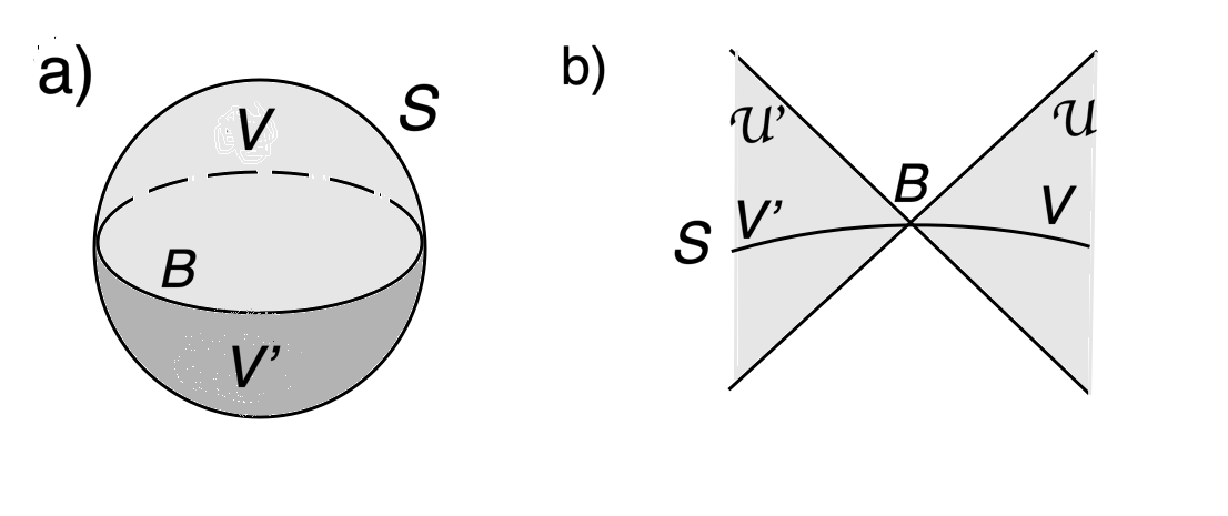
Figure 1: (a) A Cauchy hypersurface $S$, drawn as a two-sphere, is divided by the equator $B$ into an upper hemisphere $V$ and a lower hemisphere $V^{\prime}$. (b) In this view, $S$ is drawn as a one-dimensional curve and $B$ is depicted as a point that divides $S$ into the two open sets $V$ and $V^{\prime}$. ${\mathcal{U}}$ and ${\mathcal{U}}^{\prime}$ are open sets in spacetime that are the domains of dependence of $V$ and $V^{\prime}$. It is apparent from this picture that near $B$, ${\mathcal{U}}$ and ${\mathcal{U}}^{\prime}$ can be modeled by opposite Rindler wedges in Minkowski space.

2.5 What is Quantum Field Theory In An Open Universe?

If there is no natural Hilbert space in an open universe, what can it mean to do quantum field theory in one? Before answering this question, let us first discuss closed universes a little more. Consider an observer who has access only to a portion of a closed universe, or who wants to develop a formalism suitable to describe experiments in just a portion of the universe. We will be particularly interested in a region of spacetime of the following sort (fig. 1). Let $B$ be a closed, codimension 1 submanifold of a Cauchy hypersurface $S$, such that the complement of $B$ is the union of two disjoint open sets $V$ and $V^{\prime}$. Let ${\mathcal{U}}$ and ${\mathcal{U}}^{\prime}$ be the domains of dependence of $V$ and $V^{\prime}$, respectively. We call an open set of the form ${\mathcal{U}}$ or ${\mathcal{U}}^{\prime}$ a “local region,” and we want to know what quantum field theory says for an observer who makes observations only in such a local region.

Classically, in a relativistic field theory, fields in ${\mathcal{U}}$ are determined by initial data on $V$. Quantum mechanically, this is also true in free field theory; we exploited this fact in section 2.1. In a generic non-free quantum field theory, it is in general not possible to define observables on a spacelike surface such as $V$, and instead we thicken $V$ slightly to an open set ${\mathcal{V}}$, satisfying $V\subset{\mathcal{V}}\subset{\mathcal{U}}$. Roughly, we will describe the sense in which initial data for observations in ${\mathcal{U}}$ can be formulated in ${\mathcal{V}}$. Note that ${\mathcal{U}}$ and ${\mathcal{V}}$ are both globally hyperbolic spacetimes in their own right, with a Cauchy hyperurface – namely $V$ – which is a portion of the Cauchy hypersurface $S$ of the full spacetime $M$.

An analog in ordinary quantum mechanics of restricting from a spacetime $M$ to a local region ${\mathcal{U}}$ is to consider only a subsystem $X$ of a larger bipartite system $XY$. In ordinary quantum mechanics, the subsystems $X$ and $Y$ are described by Hilbert spaces ${\mathcal{H}}_{X}$ and ${\mathcal{H}}_{Y}$, and the composite system $XY$ is described by the tensor product ${\mathcal{H}}_{XY}={\mathcal{H}}_{X}\otimes{\mathcal{H}}_{Y}$. A general state of the full system $XY$, possibly a pure state, when restricted to the subsystem $X$, is described by a density matrix $\rho_{X}$. Here $\rho_{X}$ is a self-adjoint operator, positive and of trace 1, acting on the Hilbert space ${\mathcal{H}}_{X}$ of the subsystem. Let ${\mathscr{A}}_{X}$ be the algebra of all operators of subsystem $X$; this is the same as the algebra of all operators on ${\mathcal{H}}_{X}$. For ${\sf a}\in{\mathscr{A}}_{X}$, its expectation value in a state characterized by the density matrix $\rho_{X}$ is defined as $F({\sf a})={\rm Tr}\,\rho_{X}{\sf a}$. The function $F({\sf a})$ has three key properties, already introduced in section 2.2, which characterize what is known as a “state” on an algebra:

• it is linear in ${\sf a}$, namely $F(\lambda{\sf a}+\mu{\sf b})=\lambda F({\sf a})+\mu F({\sf b})$, for ${\sf a},{\sf b}\in{\mathscr{A}}_{X}$, $\lambda,\mu\in{\mathbb{C}}$,

• it is normalized to $F(1)=1$,

• it is positive, in the sense that $F({\sf a}^{\dagger}{\sf a})\geq 0$ for all ${\sf a}\in{\mathscr{A}}_{X}$.

So a density matrix $\rho_{X}$ for the subsystem $X$ is a state on the algebra ${\mathscr{A}}_{X}$ consisting of all operators on the Hilbert space ${\mathcal{H}}_{X}$ of subsystem $X$.

In quantum field theory, there is no way to associate a Hilbert space to a local region in spacetime. The best one can do is to associate to an open set ${\mathcal{W}}\subset M$ a corresponding algebra of operators ${\mathscr{A}}_{\mathcal{W}}$. The algebras ${\mathscr{A}}_{\mathcal{W}}$ obey physically motivated axioms, such as a condition associated to causality: ${\mathscr{A}}_{\mathcal{W}}$ and ${\mathscr{A}}_{{\mathcal{W}}^{\prime}}$ commute (in the ${\mathbb{Z}}_{2}$-graded sense if fermions are present) if the regions ${\mathcal{W}}$ and ${\mathcal{W}}^{\prime}$ are spacelike separated. We will discuss in more detail presently the construction of ${\mathscr{A}}_{\mathcal{W}}$. For now, we just note a difference between a local region in quantum field theory and a subsystem in ordinary quantum mechanics: the algebra ${\mathscr{A}}_{\mathcal{W}}$ is, in the von Neumann algebra language, of Type III, not Type I [15, 16, 17, 18, 19]. This will be explained in section 3, in the analogous setting of quantum statistical mechanics. The Type III nature of the algebras is actually the reason that there is no way to associate a Hilbert space to a local region. If the algebra ${\mathscr{A}}_{\mathcal{W}}$ were of Type I, it would have an irreducible representation in a Hilbert space, and this Hilbert space would be naturally associated to the open set ${\mathcal{W}}$ in spacetime. However, a Type III algebra does not have an irreducible representation in a Hilbert space. Accordingly in quantum field theory, there is no natural way to associate a Hilbert space ${\mathcal{H}}_{\mathcal{W}}$ to an open set ${\mathcal{W}}$. All that we can really associate to the region ${\mathcal{W}}$ is the algebra ${\mathscr{A}}_{\mathcal{W}}$, not a preferred Hilbert space that it acts on.

There is also no good notion of a density matrix for the region ${\mathcal{W}}$, since this notion is not applicable for a Type III algebra. But the notion of a state of the algebra ${\mathscr{A}}_{\mathcal{W}}$ – a linear function obeying conditions that were stated previously – does make sense. This is the appropriate analog in quantum field theory of the notion of the density matrix of a subsystem in ordinary quantum mechanics.

With this in mind, what should quantum dynamics mean for a local region ${\mathcal{U}}\subset M$? We assume as described earlier that ${\mathcal{U}}$ is the domain of dependence of some set $V$, which has a slight thickening to an open set ${\mathcal{V}}\subset{\mathcal{U}}$. If we could associate a Hilbert space to quantum fields on $V$ or in ${\mathcal{V}}$, we could describe quantum dynamics in terms of state vectors. We would say that a quantum state that defines initial conditions on $V$ or in ${\mathcal{V}}$ actually determines the probabilities for measurement outcomes in the larger region ${\mathcal{U}}$. Since instead we only have algebras of operators associated to ${\mathcal{V}}$ and ${\mathcal{U}}$, we have to say something similar in terms of algebras. The necessary statement is just that in a quantum field theory, in this situation ${\mathscr{A}}_{\mathcal{U}}={\mathscr{A}}_{\mathcal{V}}$, meaning that operators in region ${\mathcal{U}}$ are actually equivalent to operators in region ${\mathcal{V}}$ (although simple operators in region ${\mathcal{U}}$ might correspond to rather complicated operators in the smaller region ${\mathcal{V}}$). Since ${\mathscr{A}}_{\mathcal{U}}={\mathscr{A}}_{\mathcal{V}}$, a state of ${\mathscr{A}}_{\mathcal{V}}$ is automatically a state of ${\mathscr{A}}_{\mathcal{U}}$: in other words, the data needed to predict measurements outcomes in region ${\mathcal{V}}$ (to the extent that such outcomes are predictable in quantum mechanics) also suffice to predict measurement outcomes in the larger region ${\mathcal{U}}$. The statement that ${\mathscr{A}}_{\mathcal{U}}={\mathscr{A}}_{\mathcal{V}}$, together with general axioms about the local algebras, such as those described in [12, 17], is the content of quantum dynamics for a local region.

Now let us discuss in more detail the definition of the algebra ${\mathscr{A}}_{\mathcal{W}}$ associated to an open set ${\mathcal{W}}$. We assume to begin with that ${\mathcal{W}}$ is contained in a closed universe $M$, or at least in some spacetime (such as Minkowski space) to which the quantum field theory of interest associates a Hilbert space ${\mathcal{H}}$. A standard approach to defining ${\mathscr{A}}_{\mathcal{W}}$ is as follows. Let ${\mathcal{O}}(x)$ be a local operator of the quantum field theory in question, and $f$ a smooth function with compact support in ${\mathcal{W}}$. Then $K_{f}=\exp({\mathrm{i}}\int_{\mathcal{W}}{\mathrm{d}}^{D}x\sqrt{g}f(x){\mathcal{O}}(x))$ is a bounded operator on ${\mathcal{H}}$. ${\mathscr{A}}_{\mathcal{W}}$ is then defined as the von Neumann algebra generated by such operators on ${\mathcal{H}}$.

The purpose of introducing the global Hilbert space ${\mathcal{H}}$ was to make sure that expressions such as $K_{f}$ can be interpreted as Hilbert space operators so that it is possible to take weak limits and define a von Neumann algebra. The von Neumann algebra language is useful because it makes possible simple statements such as ${\mathscr{A}}_{\mathcal{U}}={\mathscr{A}}_{\mathcal{V}}$ (which would not hold if we do not complete the algebras by taking weak limits). However, this language has the drawback of not directly incorporating the operator product expansion (OPE), which is an important statement of the locality of quantum field theory. One approach to incorporating the OPE is to enrich the von Neumann algebra language with a further axiom which would imply the existence of an OPE [28]. Another approach is to state axioms for quantum field theory in curved spacetime that directly incorporate the OPE [11]. In some approaches, the notion of a state has to be refined to incorporate the expected short distance singularities of the quantum field theory under study, but it is preferable if (as in [11]) the expected short distance behavior can be built into the structure of the algebra. The best treatment of such questions is not entirely clear in the author’s opinion, and in this article we will not adopt any particular point of view.

Before discussing an open universe, we need a few more facts about local regions in a closed universe $M$. Let us specialize to the case of an open set that is a local region ${\mathcal{U}}\subset M$, or a smaller open set ${\mathcal{V}}\subset{\mathcal{U}}$, as described earlier. Thus ${\mathcal{U}}$ or ${\mathcal{V}}$ is globally hyperbolic, with a Cauchy hypersurface $V$ that is an open subset of a Cauchy hypersurface $S$ of $M$. There are many ways to embed ${\mathcal{U}}$ or ${\mathcal{V}}$ in some other closed universe $M^{\prime}$, such that $V$ is an open subset of a Cauchy hypersurface $S^{\prime}$ of $M^{\prime}$. For this, we simply modify $S$ outside of $V$, or $M$ outside of ${\mathcal{U}}$ or ${\mathcal{V}}$. However, ${\mathscr{A}}_{\mathcal{U}}$ and ${\mathscr{A}}_{\mathcal{V}}$ depend only on ${\mathcal{U}}$ and ${\mathcal{V}}$, and not on how ${\mathcal{U}}$ and ${\mathcal{V}}$ have been embedded in $M$. This has been called “the principle of locality” [6]. For free field theory, the statement is a theorem. In general, it is expected to hold because the algebras ${\mathscr{A}}_{\mathcal{U}}$ and ${\mathscr{A}}_{\mathcal{V}}$ are ultimately determined by operator product relations in the regions ${\mathcal{U}}$ and ${\mathcal{V}}$, and these relations are entirely local in nature. The principle of locality is analogous to what we learned about spin systems in section 2.2: there are many inequivalent representations of the algebra of an infinite collection of spins, but they are all equivalent for any finite set of spins.

Given the principle of locality, we can explain the meaning of quantum field theory in an open universe $M^{\prime}$, now with a noncompact initial value surface $S^{\prime}$. Let $V\subset S^{\prime}$ be an open set that is small enough that it can be embedded in a closed manifold $\widetilde{V}$. Let ${\mathcal{U}}$ be the domain of dependence of $V$ in $M^{\prime}$, and ${\mathcal{V}}\subset{\mathcal{U}}$ a small thickening of $V$. Because $V$ can be embedded in the compact manifold $\widetilde{V}$, ${\mathcal{U}}$ and ${\mathcal{V}}$ can be embedded in a closed universe $\widetilde{M}$, with $\widetilde{V}$ as Cauchy hypersurface. Then we can define algebras ${\mathscr{A}}_{\mathcal{U}}$ and ${\mathscr{A}}_{\mathcal{V}}$ associated to ${\mathcal{U}}$ and ${\mathcal{V}}$, and the principle of locality says that these local algebras depend only on ${\mathcal{U}}$ and ${\mathcal{V}}$ and not on the embedding in $M^{\prime}$. The dynamical principle of a quantum field theory is now again ${\mathscr{A}}_{\mathcal{U}}={\mathscr{A}}_{\mathcal{V}}$. This, along with general axioms about the algebras associated to open sets, is the content of quantum field theory in an open universe.

The principle of locality sheds light on what happens if we prefer to describe physics in an open universe using a Hilbert space. The only problem with doing so is that in an open universe there are many inequivalent choices of a Hilbert space and generically there is no preferred way to choose one. However, the principle of locality says that the algebra ${\mathscr{A}}_{\mathcal{U}}$ of a local region and the dynamical principle ${\mathscr{A}}_{\mathcal{U}}={\mathscr{A}}_{\mathcal{V}}$ do not depend on the choice of a Hilbert space. Because of the principle of locality, an observer interested in physics in a bounded portion of the universe may decide that the choice of a global Hilbert space from among the myriad possibilities is irrelevant. But one can pick whichever Hilbert space one wishes without changing the predictions of a theory for local dynamics.

In an open universe that obeys special asymptotic conditions at spatial infinity, one can say more. One particularly important case is an asymptotically flat universe, that is a universe that is asymptotic at spatial infinity to Minkowski space. In the asymptotically flat case, we will assume that the theory of interest has a mass gap, for a reason explained in the next paragraph. Another important case is an asymptotically Anti de Sitter (AAdS) universe, that is, a universe that is asymptotic at spatial infinity to Anti de Sitter space. In the AAdS case, one assumes a boundary condition at spatial infinity of the sort usually considered in the AdS/CFT correspondence. An asymptotically flat or AAdS spacetime is time-independent for modes near spatial infinity, so one has a natural separation in positive and negative frequencies for modes near spatial infinity. For any mode of sufficiently short wavelength, there is a natural separation in positive and negative frequencies. In short, for the modes that either have short wavelength or are located near spatial infinity – which means for all but finitely many modes – there is a natural asymptotic separation in positive and negative frequencies. Hence, an asymptotically flat or AAdS spacetime (with a mass gap in the asymptotically flat case) is similar to a closed universe: there is a natural treatment asymptotically for all but finitely many modes, and therefore we should expect that a natural Hilbert space will exist.

Clearly, the argument as stated in the last paragraph is only heuristic, and I am not aware of precise theorems in the literature. For a quantum field theory with a mass gap $m$, the effects of spacetime curvature on the ground state are exponentially small in the limit that the radius of curvature is large compared to $1/m$. In such a case, in an asymptotically flat spacetime, the separation in positive and negative frequencies becomes exponentially precise near spatial infinity, where the radius of curvature diverges, so there should be no difficulty. In AAdS space with the usual sort of boundary conditions, there are no infrared issues and this case should also be safe. The delicate case is a massless theory in an asymptotically flat spacetime. For a free Maxwell field in Minkowski space, there is a natural quantization that leads to a Hilbert space with a Poincaré invariant vacuum, but this quantization is not truly unique because of the possibility of “soft hair” [29]; after coupling to charged fields, usually assumed to be massive, the soft hair plays an important role in understanding infrared divergences, soft theorems, and the memory effect [30]. With massless charged fields, the non-uniqueness of quantization becomes truly essential; moreover this has a very interesting analog for General Relativity in an asymptotically flat spacetime [31]. One cannot expect quantum field theory in an asymptotically flat spacetime to be simpler than quantum field theory in Minkowski space. So in general, a straightforward Hilbert space description of quantum field theory in asymptotically flat spacetime is only available for massive theories or possibly for massless theories whose infrared behavior is such that the $S$-matrix can be defined in a conventional Fock space.

2.6 Non-Free Theories

So far we have discussed free theories. We will add a few words on non-free theories.

One of the main criteria for successful quantization of a free theory is that correlation functions such as the two-point function $\langle\Psi|\phi(\vec{x},t)\phi(\vec{x}^{\prime},t^{\prime})|\chi\rangle$ should have standard short distance singularities. A two-point function with that property is the essential input to perturbation theory. So one would expect, modulo some well-understood issues of anomaly cancellation, that weakly coupled theories make sense in perturbation theory when free theories do. See [32, 33] for some rigorous results.

One would anticipate that the same is true nonperturbatively, for theories such as QCD. If a theory exists perturbatively in curved spacetime, and nonperturbatively in flat spacetime, one would expect that it works nonperturbatively in curved spacetime. Unfortunately, not much is available in terms of rigorous theorems, except for special models like two-dimensional conformal field theories. That reflects the general mathematical difficulty of understanding quantum field theory rigorously. One would think that rigorous results for a superrenormalizable theory in curved spacetime might be relatively accessible, but such results are not available.

3 Quantum Statistical Mechanics and the Thermodynamic Limit

3.1 The Thermofield Double

In this section, we will consider a simpler problem that is actually somewhat analogous to quantum field theory in an open universe. Instead of quantum field theory in curved spacetime, we consider quantum statistical mechanics at positive temperature $T=1/\beta$. In finite volume, there is no problem. We just consider the density matrix $\rho=\frac{1}{Z}e^{-\beta H}$ acting on the Hilbert space ${\mathcal{H}}$ of the system, where $Z={\rm Tr}\,e^{-\beta H}$ is the partition function. Importantly, for any conventional statistical system (possibly a relativistic quantum field theory, possibly a nonrelativistic system of some kind), the partition function converges in finite volume. Thermodynamic functions and thermal correlation functions can all be computed in finite volume, and they have a thermodynamic or large volume limit.

What happens if one wants to describe the thermodynamic limit of a system directly in terms of operators acting on a Hilbert space appropriate for an infinite volume system? Here we run into a difficulty: there is no separable Hilbert space that contains all the typical states of a system at $T\not=0$, since fluctuations can occur throughout the whole infinite space. For example, for a spin system on an infinite lattice, since each spin has a nonzero probability to fluctuate, it takes uncountably many states to describe all the typical states at $T\not=0$. (We discuss some examples based on lattice spin systems in section 3.3.) In a continuum field theory, there is actually no reasonable definition of a nonseparable Hilbert space that contains all the typical thermal excitations in infinite volume.

There is a simple device that enables one to describe the thermodynamic limit of any quantum system in a separable Hilbert space [20]. This is the “thermofield double.” Consider an ordinary quantum system ${\mathcal{T}}$ (possibly a relativistic field theory, possibly a lattice theory or something else) with Hilbert space ${\mathcal{H}}$ and Hamiltonian $H$. In finite volume, the thermofield double is defined by introducing, roughly speaking, two copies of the original system, which we will call the “right” and “left” copies, with Hilbert spaces ${\mathcal{H}}_{r}$ and ${\mathcal{H}}_{\ell}$, and Hamiltonians $H_{r}$ and $H_{\ell}$. We think of ${\mathcal{H}}_{r}$ as the Hilbert space of the system ${\mathcal{T}}$ and ${\mathcal{H}}_{\ell}$ as an auxiliary second copy. Actually, rather than being a second copy of ${\mathcal{H}}_{r}$, it is more canonical to define ${\mathcal{H}}_{\ell}$ to be the complex conjugate Hilbert space of ${\mathcal{H}}_{r}$. That amounts physically to saying that the left system is a time-reversal conjugate of the right system (rather than being an identical second copy). The fact that ${\mathcal{H}}_{\ell}$ is the complex conjugate of ${\mathcal{H}}_{r}$ ensures that the combined Hilbert space ${\mathcal{H}}_{\mathrm{TFD}}={\mathcal{H}}_{\ell}\otimes{\mathcal{H}}_{r}$ of the two systems can be viewed canonically as the space of linear operators acting on ${\mathcal{H}}_{r}$ (or ${\mathcal{H}}_{\ell}$). In expositions of the thermofield double, time-reversal symmetry is often assumed, in which case the left and right systems are equivalent.

In finite volume, the thermofield double $\Psi_{\mathrm{TFD}}$ is simply a vector in ${\mathcal{H}}_{\ell}\otimes{\mathcal{H}}_{r}$, defined as follows. Suppose that the Hamiltonian acting on the original system has eigenstates $\psi_{i}$ with energies $E_{i}$. Then in finite volume, $\Psi_{\mathrm{TFD}}$ is defined as

$$\Psi_{\mathrm{TFD}}=\frac{1}{\sqrt{Z}}\sum_{i}\exp(-\beta E_{i}/2)|\overline{i}\rangle_{\ell}\otimes|i\rangle_{r},$$ (3.1)

Here $|i\rangle_{r}$ is the $i^{th}$ energy level of the right system, with energy $E_{i}$; $|\overline{i}\rangle_{\ell}$ is its time-reversal conjugate in the left system; and $Z$ is the partition function of the right or left system at temperature $1/\beta$. The point of this formula is that the density matrix of the right or left system is the usual thermal density matrix of that system:

$$\rho_{r}={\rm Tr}_{{\mathcal{H}}_{\ell}}|\Psi_{\mathrm{TFD}}\rangle\langle\Psi_{\mathrm{TFD}}|=\frac{1}{Z}\sum_{i}e^{-\beta E_{i}}|i\rangle_{r}\langle i|_{r}=\frac{1}{Z}e^{-\beta H_{r}}.$$ (3.2)

So the thermofield double is a “purification” of a thermal density matrix.

An equivalent statement is the following. If we view ${\mathcal{H}}_{\ell}\otimes{\mathcal{H}}_{r}$ as the space of linear operators acting on ${\mathcal{H}}_{r}$, then $\Psi_{\mathrm{TFD}}=\rho_{r}^{1/2}$. To exploit this fact, let ${\mathscr{A}}_{r,V}$ and ${\mathscr{A}}_{\ell,V}$ be the algebras of all operators acting on ${\mathcal{H}}_{r}$ or ${\mathcal{H}}_{\ell}$, respectively, in finite volume $V$. Viewing a state vector $\Psi\in{\mathcal{H}}_{\ell}\otimes{\mathcal{H}}_{r}$ as a matrix acting on ${\mathcal{H}}_{r}$, an element ${\sf a}_{r}\in{\mathscr{A}}_{r,V}$ acts on $\Psi$ by $\Psi\to{\sf a}_{r}\Psi$, and an element ${\sf a}_{\ell}\in{\mathscr{A}}_{\ell,V}$ acts on $\Psi$ by $\Psi\to\Psi{\sf a}_{\ell}^{\mathrm{tr}}$ (where ${\sf a}_{\ell}^{\mathrm{tr}}$ is the transpose of ${\sf a}_{\ell}$). If $\Psi$, viewed as a matrix acting on ${\mathcal{H}}_{r}$, is invertible, then every matrix acting on ${\mathcal{H}}_{r}$ is of the form ${\sf a}_{r}\Psi$ and of the form $\Psi{\sf a}_{\ell}^{\mathrm{tr}}$ for some unique ${\sf a}_{r}\in{\mathscr{A}}_{r,V}$ and for some unique ${\sf a}_{\ell}\in{\mathscr{A}}_{\ell,V}$. In particular, $\Psi_{\mathrm{TFD}}=\rho_{r}^{1/2}$ is invertible, and therefore every vector in ${\mathcal{H}}_{\mathrm{TFD}}$ can be obtained from $\Psi_{\mathrm{TFD}}$ by acting with ${\mathscr{A}}_{r,V}$, or by acting with ${\mathscr{A}}_{\ell,V}$. The fancy way to say this is that if $\Psi$ is invertible, then it corresponds to a cyclic separating vector for the algebras ${\mathscr{A}}_{r,V}$ and ${\mathscr{A}}_{\ell,V}$.

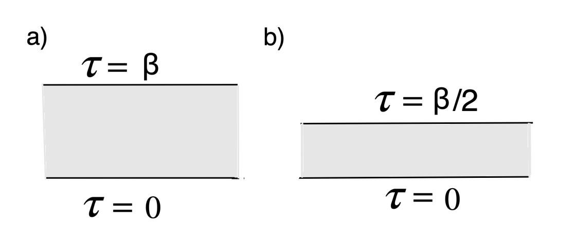
Figure 2: (a) A thermal density matrix $\rho=\frac{1}{Z}e^{-\beta H}$ can be computed by a path integral on the strip $0\leq\tau\leq\beta$. The horizontal direction in the picture represents the “spatial” manifold (or lattice) $W$. (b) The thermofield double state $\Psi_{\mathrm{TFD}}=\rho^{1/2}$ can be computed by a path integral on a strip of half the width, $0\leq\tau\leq\beta/2$. Operators of the “right” or “left” copy are inserted, respectively, on the boundaries at $\tau=0$ and $\tau=\beta/2$. .

We want to take the infinite volume limit of this construction. As already noted, the left and right Hilbert spaces ${\mathcal{H}}_{r}$ and ${\mathcal{H}}_{\ell}$ do not have large volume limits, and the formula (3.1) is not meaningful in the thermodynamic limit, because $Z=\infty$ in this limit and the sum would contain uncountably many terms. But it is possible to define a Hilbert space ${\mathcal{H}}_{\mathrm{TFD}}$ that contains $\Psi_{\mathrm{TFD}}$ and does have a large volume limit. To explain this, we first review a few standard facts about finite volume. We describe these facts in the familiar language of path integrals, though this is not strictly necessary. Let $W$ be the spatial manifold (or lattice) on which we want to formulate theory ${\mathcal{T}}$. In the thermodynamic limit, $W$ will be ${\mathbb{R}}^{D-1}$ for a continuum field theory or an infinite lattice ${\mathbb{Z}}^{D-1}$ for a lattice system. The thermal density matrix $\rho_{r}=\frac{1}{Z}e^{-\beta H}$ can be computed in finite volume by a path integral on $W\times I$, where $I$ is the interval $0\leq\tau\leq\beta$ (fig. 2) The factor of $1/Z$ means that from the energy density $T_{00}$, whose integral is the Hamiltonian $H_{r}=\int{\mathrm{d}}^{D-1}x\sqrt{g}T_{00}$, we should subtract a constant, the free energy density at temperature $1/\beta$. With this subtraction, the path integral, in finite volume, computes a normalized density matrix $\rho_{r}$, satisfying ${\rm Tr}\,\rho_{r}=1$. To construct the thermofield double state $\Psi_{\mathrm{TFD}}=\rho_{r}^{1/2}$, we simply do the same path integral (with the same subtraction) on a strip of half the width, $0\leq\tau\leq\beta/2$. Given an operator ${\sf a}_{r}\in{\mathscr{A}}_{r,V}$, to construct a state obtained by acting with ${\sf a}_{r}$ on $\Psi_{\mathrm{TFD}}$, we just insert ${\sf a}_{r}$ in the path integral at $\tau=0$; similarly, to act with ${\sf a}_{\ell}\in{\mathscr{A}}_{\ell,V}$ on $\Psi_{\mathrm{TFD}}$, we insert ${\sf a}_{\ell}^{\mathrm{tr}}$ at $\tau=\beta/2$. Inner products between these states are computed by gluing together two path integrals on the strip of width $\beta/2$ to make a cylinder of circumference $\beta$. For example, an inner product $\langle{\sf b}_{r}\Psi_{\mathrm{TFD}}|{\sf a}_{r}\Psi_{\mathrm{TFD}}\rangle=\langle\Psi_{\mathrm{TFD}}|{\sf b}_{r}^{\dagger}{\sf a}_{r}\Psi_{\mathrm{TFD}}\rangle$ is computed by a path integral on the cylinder with insertion of ${\sf b}_{r}^{\dagger}{\sf a}_{r}$ at $\tau=0$. This quantity is just the expectation value of ${\sf b}_{r}^{\dagger}{\sf a}_{r}$ in the thermal ensemble:

$$\langle{\sf b}_{r}\Psi_{\mathrm{TFD}}|{\sf a}_{r}\Psi_{\mathrm{TFD}}\rangle=\langle\Psi_{\mathrm{TFD}}|{\sf b}_{r}^{\dagger}{\sf a}_{r}|\Psi_{\mathrm{TFD}}\rangle={\rm Tr}\,\rho_{r}{\sf b}_{r}^{\dagger}{\sf a}_{r}=\frac{1}{Z}{\rm Tr}_{{\mathcal{H}}_{r}}\exp(-\beta H_{r}){\sf b}_{r}^{\dagger}{\sf a}_{r}.$$ (3.3)

Such thermal expectation values have a thermodynamic limit. Since the density operator $\rho_{r}$ is strictly positive, one has

$$\langle{\sf a}_{r}\Psi_{\mathrm{TFD}}|{\sf a}_{r}\Psi_{\mathrm{TFD}}\rangle={\rm Tr}_{{\mathcal{H}}_{r}}\rho_{r}{\sf a}_{r}^{\dagger}{\sf a}_{r}>0$$ (3.4)

for all ${\sf a}_{r}\not=0$. Likewise, for ${\sf a}_{\ell}\not=0$, we can construct states ${\sf a}_{\ell}\Psi_{\mathrm{TFD}}$ by acting with ${\sf a}_{\ell}^{\mathrm{tr}}$ at $\tau=\beta/2$. Inner products between these states are obviously given by a formula like eqn. (3.3) which again has a thermodynamic limit:

$$\langle{\sf b}_{\ell}\Psi_{\mathrm{TFD}}|{\sf a}_{\ell}\Psi_{\mathrm{TFD}}\rangle=\frac{1}{Z}{\rm Tr}_{{\mathcal{H}}_{\ell}}\exp(-\beta H_{\ell}){\sf b}_{\ell}^{\dagger}{\sf a}_{\ell}.$$ (3.5)

Inner products $\langle{\sf a}_{\ell}\Psi_{\mathrm{TFD}}|{\sf a}_{r}\Psi_{\mathrm{TFD}}\rangle$ are defined by inserting the operators ${\sf a}_{r}$ and $({\sf a}_{\ell}^{\mathrm{tr}})^{\dagger}={\sf a}_{\ell}^{*}$ (here ${\sf a}_{\ell}^{*}$ is the complex conjugate of ${\sf a}_{\ell}$; note that because of the complex conjugation, it is naturally an operator on ${\mathcal{H}}_{r}$) at $\beta=0$ and $\beta=\tau/2$, respectively. In operator terms, such an inner product is

$$\langle{\sf a}_{\ell}\Psi_{\mathrm{TFD}}|{\sf a}_{r}\Psi_{\mathrm{TFD}}\rangle=\frac{1}{Z}{\rm Tr}_{{\mathcal{H}}_{r}}\,{\sf a}_{r}e^{-\beta H_{r}/2}{\sf a}_{\ell}^{*}e^{-\beta H_{r}/2}.$$ (3.6)

Such an inner product also has a thermodynamic limit. Reflection positivity says that for any ${\sf a}_{\ell}$, there is an ${\sf a}_{r}$ that makes this inner product nonzero. We simply choose ${\sf a}_{r}$ to be obtained from ${\sf a}_{\ell}$ by a reflection of the thermal circle.

In finite volume, the states that appeared in this construction are simply states in ${\mathcal{H}}_{\ell}\otimes{\mathcal{H}}_{r}$. In the infinite volume limit, this is no longer true. But now we can describe a Hilbert space ${\mathcal{H}}_{\mathrm{TFD}}$ that does have a thermodynamic limit. First we need to pick an algebra of operators that is supposed to act on ${\mathcal{H}}_{\mathrm{TFD}}$. As in section 2.2, we at least want to include all operators that act on a bounded region of space. Ultimately we can take limits and include operators whose action is not restricted to a bounded region, but to know what limits to allow, we first have to know what Hilbert space the operators are supposed to act on. So we define algebras ${\mathscr{A}}_{r,0}$ and ${\mathscr{A}}_{\ell,0}$ consisting of bounded operators acting on a bounded region in the right system or the left system, respectively. Now at a minimum we want ${\mathcal{H}}_{\mathrm{TFD}}$ to contain a vector that we call $\Psi_{\mathrm{TFD}}$ which will be an infinite volume limit of the finite volume thermofield double state. In addition, we want the algebras ${\mathscr{A}}_{r,0}$ and ${\mathscr{A}}_{\ell,0}$ to act on ${\mathcal{H}}_{\mathrm{TFD}}$. So we say that for every ${\sf a}_{r}\in{\mathscr{A}}_{r,0}$, ${\mathcal{H}}_{\mathrm{TFD}}$ contains a vector that we call ${\sf a}_{r}\Psi_{\mathrm{TFD}}$. ${\mathscr{A}}_{r,0}$ acts on these states in an obvious way: ${\sf a}_{r}({\sf b}_{r}\Psi_{\mathrm{TFD}})=({\sf a}_{r}{\sf b}_{r})\Psi_{\mathrm{TFD}}$. We postulate that the inner products between these states are given by the thermodynamic limit of the thermal correlation functions in eqn. (3.3). Because of eqn. (3.4), this set of states makes up a pre-Hilbert space ${\mathcal{H}}_{{\mathrm{TFD}},0}$, satisfying all conditions of a Hilbert space except completeness. We take the Hilbert space completion and get the thermofield double Hilbert space ${\mathcal{H}}_{\mathrm{TFD}}$. We can now also complete ${\mathscr{A}}_{r,0}$ to a von Neumann algebra ${\mathscr{A}}_{r}$ that acts on ${\mathcal{H}}_{\mathrm{TFD}}$ by including weak limits, as in section 2.2.

Obviously, we could have carried out this process starting with ${\mathscr{A}}_{\ell,0}$ instead of ${\mathscr{A}}_{r,0}$. One might worry that this would lead to a different thermofield double Hilbert space $\widetilde{\mathcal{H}}_{\mathrm{TFD}}$, with an action of a left algebra ${\mathscr{A}}_{\ell}$ instead of ${\mathscr{A}}_{r}$. The reason that this does not happen is that the formula eqn. (3.6) for inner products between states ${\sf a}_{\ell}\Psi_{\mathrm{TFD}}$ and states ${\sf a}_{r}\Psi_{\mathrm{TFD}}$ also has a thermodynamic limit and implies that ${\sf a}_{\ell}\Psi_{\mathrm{TFD}}$ can be viewed as a vector in the same Hilbert space ${\mathcal{H}}_{\mathrm{TFD}}$ that we defined starting with states ${\sf a}_{r}\Psi_{\mathrm{TFD}}$.

The upshot is to define a Hilbert space ${\mathcal{H}}_{\mathrm{TFD}}$ with an action of completions ${\mathscr{A}}_{\ell}$ and ${\mathscr{A}}_{r}$ of ${\mathscr{A}}_{\ell,0}$ and ${\mathscr{A}}_{r,0}$. Inner products between vectors of the form ${\sf a}_{\ell}\Psi_{\mathrm{TFD}}$ and/or ${\sf a}_{r}\Psi_{\mathrm{TFD}}$ are defined via the thermodynamic limits of eqns. (3.3), (3.5), and (3.6). All expected relations among inner products between Hilbert space vectors are satisfied, because we are simply taking the thermodynamic limits of formulas that in finite volume do represent inner products between Hilbert space vectors. Moreover, in terminology that was defined in footnote 12, $\Psi_{\mathrm{TFD}}\in{\mathcal{H}}_{{\mathrm{TFD}}}$ is always a cyclic separating vector for the algebra ${\mathscr{A}}_{r}$ (or ${\mathscr{A}}_{\ell}$).

The procedure by which we constructed the thermodynamic limit of ${\mathcal{H}}_{\mathrm{TFD}}$ is a special case of the Gelfand-Naimark-Segal (GNS) construction in which the input is an algebra ${\mathscr{A}}$ and a state on the algebra, that is a complex-valued linear function ${\sf a}\to F({\sf a})$ such that $F(1)=1$ and $F({\sf a}^{\dagger}{\sf a})>0$ for all ${\sf a}\not=0$, and the output is a Hilbert space ${\mathcal{H}}$ with an action of ${\mathscr{A}}$ and a cyclic separating vector $\Psi$. (Closely related is the Wightman Reconstruction Theorem of axiomatic field theory, in which a Hilbert space is reconstructed from the correlation functions of a local field.) The GNS construction proceeds as follows. One formally associates a vector $\Psi$ to the identity element $1\in{\mathscr{A}}$, and to every ${\sf a}\in{\mathscr{A}}$ one associates a vector ${\sf a}\Psi$. The action of ${\mathscr{A}}$ on this set of states is defined in the obvious way by ${\sf a}({\sf b}\Psi)=({\sf a}{\sf b})\Psi$, and inner products are defined by $\langle{\sf a}\Psi|{\sf b}\Psi\rangle=F({\sf a}^{\dagger}{\sf b})$. This gives a pre-Hilbert space ${\mathcal{H}}_{0}$ with an action of ${\mathscr{A}}$, and one completes it to a Hilbert space ${\mathcal{H}}$. From the definitions, it is immediate that ${\mathscr{A}}$ acts on ${\mathcal{H}}$ with $\Psi$ as a cyclic separating vector. Clearly the definition of ${\mathcal{H}}_{\mathrm{TFD}}$ is the GNS construction applied to the case that $F({\sf a})$ is the expectation value of ${\sf a}$ in the thermodynamic limit.

3.2 Surprises In The Thermodynamic Limit

So by going to the thermofield double, we can describe the infinite volume limit of quantum statistical mechanics in a separable Hilbert space ${\mathcal{H}}_{\mathrm{TFD}}$. But there are a few surprises.

First of all, evidently ${\mathscr{A}}_{r}$ does not act irreducibly on ${\mathcal{H}}_{\mathrm{TFD}}$, since it commutes with ${\mathscr{A}}_{\ell}$, and vice-versa. In fact ${\mathscr{A}}_{\ell}$ and ${\mathscr{A}}_{r}$ are algebras of a possibly unfamiliar kind: they are generically von Neumann algebras of Type III. What characterizes algebras of Type II or Type III, as opposed to the more familiar algebras of Type I, is roughly that entanglement is not just a property of the states that the algebra acts on but is built into the structure of the algebra. In finite volume $V$, the entanglement entropy of the state $\Psi_{\mathrm{TFD}}\in{\mathcal{H}}_{\ell}\otimes{\mathcal{H}}_{r}$ is the same as the thermodynamic entropy of the thermal density matrix $\rho_{r}$ or $\rho_{\ell}$ on one factor. In particular, it is proportional to $V$ and diverges in the thermodynamic limit. Thus in effect $\Psi_{{\mathrm{TFD}}}$ in the thermodynamic limit describes a state with an infinite entanglement between the two systems. But every state in ${\mathcal{H}}_{\mathrm{TFD}}$ looks at spatial infinity like $\Psi_{\mathrm{TFD}}$ and so every state has the same divergent entanglement entropy. This is different from the usual situation for a bipartite quantum system $XY$ with Hilbert space ${\mathcal{H}}_{XY}={\mathcal{H}}_{X}\otimes{\mathcal{H}}_{Y}$ where ${\mathcal{H}}_{X}$ and ${\mathcal{H}}_{Y}$ are of infinite dimension. In such a case, a vector $\Psi_{XY}\in{\mathcal{H}}_{XY}$ could have infinite entanglement entropy, but there are also vectors in ${\mathcal{H}}_{XY}$ with finite or zero entanglement entropy. By contrast, in the infinite volume limit, ${\mathcal{H}}_{\mathrm{TFD}}$ is not a tensor product and no vector in it can be interpreted to have finite entanglement entropy; rather, the infinite entanglement entropy between the left and right systems is encoded in the structure of the algebras ${\mathscr{A}}_{\ell}$ and ${\mathscr{A}}_{r}$. We will discuss this more thoroughly in section 3.3 with simple examples.

A second unusual property of the infinite volume thermofield double comes to light if we think about real time thermal physics. In finite volume, to study real time thermal physics, we define the time-dependence of operators in a familiar way:

$${\sf a}_{r}(t) =\exp({\mathrm{i}}H_{r}t){\sf a}_{r}\exp(-{\mathrm{i}}H_{r}t)$$ (3.7)

$${\sf a}_{\ell}(t) =\exp({\mathrm{i}}H_{\ell}t){\sf a}_{\ell}\exp(-{\mathrm{i}}H_{\ell}t).$$ (3.8)

Then we define real time correlation functions such as

$$\langle{\sf a}_{r}(t_{1}){\sf b}_{r}(t_{2})\rangle={\rm Tr}\,\rho_{r}{\sf a}_{r}(t_{1}){\sf b}_{r}(t_{2}).$$ (3.9)

These functions have a thermodynamic limit. How do we describe them using the thermofield double? A subtlety arises here: the Hamiltonians $H_{\ell}$ and $H_{r}$ of the left and right system do not make sense as operators on the infinite volume ${\mathcal{H}}_{\mathrm{TFD}}$. This is so because of thermal fluctuations. In volume $V$, the typical energy in the thermal ensemble is of course proportional to $V$, so the Hamiltonian diverges for $V\to\infty$. That in itself is not a problem, because we can “renormalize” $H_{\ell}$ and $H_{r}$ by subtracting a multiple of $V$ to get an operator whose expectation value vanishes for $V\to\infty$. The problem comes from the thermal fluctuations. The typical fluctuations in $H_{\ell}$ and $H_{r}$ in volume $V$ are of order $V^{1/2}$, which also diverges for $V\to\infty$. Even after subtracting constants from $H_{\ell}$ and $H_{r}$ to set their expectations values in the thermal ensemble to zero, the divergent fluctuations remain, and imply that $H_{\ell}$ and $H_{r}$ do not have limits as operators on ${\mathcal{H}}_{\mathrm{TFD}}$.

So how are we going to define real time correlation functions? The answer is that the operator $\widehat{H}=H_{r}-H_{\ell}$ does have a thermodynamic limit as an operator on ${\mathcal{H}}_{\mathrm{TFD}}$. This results from the fact that in finite volume $\widehat{H}$ annihilates $\Psi_{\mathrm{TFD}}$, as is evident from the definition (3.1). With the aid of $\widehat{H}$, we can describe real time thermal physics. We define

$${\sf a}_{r}(t) =\exp({\mathrm{i}}\widehat{H}t){\sf a}_{r}\exp(-{\mathrm{i}}\widehat{H}t)$$ (3.10)

$${\sf a}_{\ell}(t) =\exp(-{\mathrm{i}}\widehat{H}t){\sf a}_{\ell}\exp({\mathrm{i}}\widehat{H}t).$$ (3.11)

The motivation for these definitions is that in finite volume they agree with the standard definitions (3.7), since $[H_{\ell},{\sf a}_{r}]=[H_{r},{\sf a}_{\ell}]=0$. In terms of these definitions, the thermodynamic limit of real time correlation functions is given by formulas such as

$$\langle{\sf a}_{\ell,r}(t_{1}){\sf b}_{\ell,r}(t_{2})\rangle=\langle\Psi_{\mathrm{TFD}}|a_{\ell,r}(t_{1})b_{\ell,r}(t_{2})|\Psi_{\mathrm{TFD}}\rangle,$$ (3.12)

where the subscripts $\ell,r$ mean that the operators can belong to either ${\mathscr{A}}_{\ell}$ or ${\mathscr{A}}_{r}$.

Since the operator $\exp({\mathrm{i}}\widehat{H}t)$ is not contained in either ${\mathscr{A}}_{\ell}$ or ${\mathscr{A}}_{r}$, it follows that time translations are a group of outer automorphisms of ${\mathscr{A}}_{\ell}$ and of ${\mathscr{A}}_{r}$. Now consider the following question. Suppose that one has access to the Hilbert space ${\mathcal{H}}_{\mathrm{TFD}}$, the state $\Psi_{\mathrm{TFD}}$, and the algebra ${\mathscr{A}}_{r}$, but one does not know how this data arose by taking a thermodynamic limit. Just from ${\mathcal{H}}_{\mathrm{TFD}}$, $\Psi_{\mathrm{TFD}}$, and ${\mathscr{A}}_{r}$, how would one identify which outer automorphism group of ${\mathscr{A}}_{r}$ corresponds to time translations? The answer to this question is given by Tomita-Takesaki theory. Here we will just state a few facts, leaving the reader to look elsewhere (for example, sections 3 and 4 of [19]) for a detailed explanation. In Tomita-Takesaki theory, to a Hilbert space ${\mathcal{H}}$, an algebra ${\mathscr{A}}$ of operators on ${\mathcal{H}}$ and a state $\Psi\in{\mathcal{H}}$ that is cyclic and separating for ${\mathscr{A}}$, one associates a modular operator $\Delta_{\Psi}$. For example, if ${\mathcal{H}}={\mathcal{H}}_{XY}={\mathcal{H}}_{X}\otimes{\mathcal{H}}_{Y}$ is the Hilbert space of a bipartite system $XY$, ${\mathscr{A}}={\mathscr{A}}_{X}$ is the algebra of operators on ${\mathcal{H}}_{X}$, and $\Psi=\Psi_{XY}$ is a vector in ${\mathcal{H}}_{XY}$, then the cyclic separating condition is that the reduced density matrices $\rho_{X}$ and $\rho_{Y}$ of $\Psi_{XY}$ are invertible, and in this case the modular operator is $\Delta_{\Psi}=\rho_{X}\otimes\rho_{Y}^{-1}$. (See eqn. (4.26) in [19], for example.) In finite volume, these conditions are satisfied by ${\mathcal{H}}={\mathcal{H}}_{\mathrm{TFD}}={\mathcal{H}}_{\ell}\otimes{\mathcal{H}}_{r}$, $\Psi=\Psi_{\mathrm{TFD}}$, ${\mathscr{A}}={\mathscr{A}}_{r}$, $\rho_{r}=\frac{1}{Z}e^{-\beta H_{r}}$, $\rho_{\ell}=\frac{1}{Z}e^{-\beta H_{\ell}}$. So $\Delta_{\Psi_{\mathrm{TFD}}}=\rho_{r}\otimes\rho_{\ell}^{-1}=\exp(-\beta\widehat{H})$. Though $\rho_{\ell}$ and $\rho_{r}$ do not have a thermodynamic limit, $\Delta_{\Psi_{\mathrm{TFD}}}$ and $\widehat{H}$ do have such a limit and the formula $\Delta_{\Psi_{\mathrm{TFD}}}=\exp(-\beta\widehat{H})$ is valid in the thermodynamic limit. So we can express $\widehat{H}$ in terms of the modular operator: $\widehat{H}=-\frac{1}{\beta}\log\Delta_{\Psi_{\mathrm{TFD}}}$.

3.3 Examples From Spin Systems

Here we will consider some concrete examples of the thermofield double construction for a system with an infinite number of degrees of freedom. As in section 2.2, we consider a countably infinite set of qubits, which we label by a positive integer $n$, making the “right” system. To study this system via the thermofield double, we introduce another infinite collection of qubits, the “left” system. We write ${\mathcal{H}}_{r,N}$ for the Hilbert space of the first $N$ qubits of the right system, and ${\mathcal{H}}_{\ell,N}$ for the analog for the left system.

We will consider extremely simple Hamiltonians of the form $H=\sum_{n=1}^{\infty}H_{n}$, where $H_{n}$ is a single-qubit Hamiltonian. One may be surprised that this case is rich enough to be interesting. In fact the various von Neumann algebras can all arise from such a construction and some of them were first discovered in this way [34, 35, 36].

The simplest Hamiltonian of all is $H=0$, so we will start with that case. Let us write $|i\rangle_{n,r}$, $i=1,2$ for the two states of the $n^{th}$ qubit of the “right” system, and $|\overline{i}\rangle_{n,\ell}$, $i=1,2$ for the time-reversed states of the $n^{th}$ qubit of the “left” system. The analog of defining the thermofield double state first in finite volume, as in eqn. (3.1), is to define the thermofield double state first for the first $N$ qubits of the right system, together with their partners in the left system. With $H=0$, the thermofield double state $\Psi_{\mathrm{TFD}}\in{\mathcal{H}}_{r,N}\otimes{\mathcal{H}}_{\ell,N}$ is just a completely entangled state of $N$ pairs of qubits:

$$\Psi_{{\mathrm{TFD}}}=\frac{1}{\sqrt{Z_{N}}}\bigotimes_{n=1}^{N}\sum_{i=1,2}|i\rangle_{n,r}\otimes|\overline{i}\rangle_{n,\ell},~{}~{}~{}Z_{N}=2^{N}.$$ (3.13)

Arranging the four states $|i\rangle_{n,r}\otimes|j,\rangle_{n,\ell}$, $i,j=1,2$ in a $2\times 2$ matrix in a fairly obvious way, we can write

$$\Psi_{\mathrm{TFD}}=\frac{1}{\sqrt{Z_{N}}}\bigotimes_{n=1}^{N}\begin{pmatrix}1&0\cr 0&1\end{pmatrix}.$$ (3.14)

Now let ${\mathscr{A}}_{r,0}$ be the algebra of all operators on the right system that act nontrivially on only finitely many qubits. If ${\sf a}_{r}\in{\mathscr{A}}_{r,0}$, then for sufficiently large $N$, we can view ${\sf a}_{r}$ as an operator on ${\mathcal{H}}_{r,N}\otimes{\mathcal{H}}_{\ell,N}$ and define $F({\sf a}_{r})=\langle\Psi_{\mathrm{TFD}}|{\sf a}_{r}|\Psi_{\mathrm{TFD}}\rangle$. For given ${\sf a}_{r}$, this definition does not depend on $N$, once $N$ is large enough so that $F({\sf a}_{r})$ is defined. So $F({\sf a}_{r})$ is well-defined for all ${\sf a}_{r}\in{\mathscr{A}}_{r,0}$. It clearly is linear in ${\sf a}_{r}$ and satisfies $F({\sf a}_{r}^{\dagger}{\sf a}_{r})>0$ for ${\sf a}_{r}\not=0$, so it defines a state on the algebra ${\mathscr{A}}_{r,0}$. So we can invoke the GNS construction, as described in section 3.1, and construct the thermofield double Hilbert space ${\mathcal{H}}_{\mathrm{TFD}}$, with an action of ${\mathscr{A}}_{r,0}$, and containing the distinguished thermofield double state $\Psi_{\mathrm{TFD}}\in{\mathcal{H}}_{\mathrm{TFD}}$.

By including weak limits, we can take the closure of ${\mathscr{A}}_{r,0}$ to get an algebrs ${\mathscr{A}}_{r}$ of bounded operators that acts on ${\mathcal{H}}_{\mathrm{TFD}}$. This is an algebra of an unfamiliar kind – a Type II von Neumann algebra. In fact, it is a Murray-von Neumann factor of Type II₁ [37]. To see that the algebra ${\mathscr{A}}_{r}$ is of an unfamiliar type, note that the function $F({\sf a}_{r})$ satisfies

$$F({\sf a}_{r}{\sf b}_{r})=F({\sf b}_{r}{\sf a}_{r}).$$ (3.15)

Thus, this function has the algebraic properties of a trace, so we will denote it as one: $F({\sf a}_{r})={\rm Tr}\,{\sf a}_{r}$. Moreover, this trace is defined (and finite) for all elements of the algebra; in particular, ${\rm Tr}\,1=1$. By contrast, the obvious example of an infinite dimensional von Neumann algebra is the algebra ${\mathscr{A}}$ of all bounded operators on a separable Hilbert space ${\mathcal{H}}$. This algebra, which is said to be of Type I_∞, does have a trace ${\rm Tr}$, but the trace is not defined for all elements of ${\mathscr{A}}$ (only for those that are “trace class”) and in particular in a Type I_∞ factor, ${\rm Tr}\,1=+\infty$. So the algebra ${\mathscr{A}}_{r}$ is something new.

Intuitively, since the Type II₁ factor ${\mathscr{A}}_{r}$ was constructed by considering an infinite collection of maximally entangled qubit pairs, an infinite amount of entanglement is built into the structure of this algebra. A Type II₁ algebra does not have an irreducible representation in a Hilbert space. We constructed a representation of the Type II₁ algebra ${\mathscr{A}}_{r}$ on the Hilbert space ${\mathcal{H}}_{\mathrm{TFD}}$, but this representation is far from irreducible, since the action of ${\mathscr{A}}_{r}$ on ${\mathcal{H}}_{\mathrm{TFD}}$ commutes with the action of another Type II₁ algebra ${\mathscr{A}}_{\ell}$ that is defined similarly, starting with operators that act only on finitely many qubits of the left system and taking limits. The algebras ${\mathscr{A}}_{r}$ and ${\mathscr{A}}_{\ell}$ commute and in fact they are each other’s commutants. As this example illustrates, when a Type II₁ algebra acts on a Hilbert space, its commutant is another Type II algebra.

Murray and von Neumann classified the Hilbert space representations of a hyperfinite Type II₁ algebra. They are labeled up to isomorphism by a regularized “dimension” $x$, which is a non-negative real number or $\infty$. ${\mathcal{H}}_{\mathrm{TFD}}$ corresponds to the case $x=1$. To construct representations with $x<1$, we use projection operators in ${\mathscr{A}}_{\ell}$. For example, for $1\leq k\leq 2^{N}$, pick a $k$-dimensional subspace $W\subset{\mathcal{H}}_{\ell,N}$, and let $\Pi:{\mathcal{H}}_{\ell,N}\to W$ be the orthogonal projection operator of ${\mathcal{H}}_{\ell,N}$ onto $W$ (tensored with the identity operator on all other qubits). The image of $\Pi$ in ${\mathcal{H}}_{\mathrm{TFD}}$ is a representation of ${\mathscr{A}}_{r}$ with $x=k/2^{N}$. All values $x<1$ are limits of this with $k,N\to\infty$. Since $x$ is additive when one takes the direct sum of two representations, any representation is the direct sum of a representation with $x<1$ and a number of copies of ${\mathcal{H}}_{\mathrm{TFD}}$. Roughly, the value of $x$ for a Hilbert space representation ${\mathcal{R}}$ of ${\mathscr{A}}_{r}$ is defined as the trace of the identity element of ${\mathscr{A}}_{r}$ in the representation ${\mathcal{R}}$. Some more detail is needed to make this precise, but anyway the existence of inequivalent representations of ${\mathscr{A}}_{r}$ is related to the fact that ${\mathscr{A}}_{r}$ has a trace.

The other hyperfinite von Neumann algebra of Type II is a Type II_∞ algebra. It can be obtained as the tensor product of a Type II₁ algebra with a Type I_∞ algebra of all bounded operators on a separable Hilbert space. It has a trace, which, because of the Type I_∞ factor, is not defined for all elements of the algebra.

Repeating this construction with a non-zero Hamiltonian, we can get the other hyperfinite von Neumann algebras. Again with $H=\sum_{n=1}^{\infty}H_{n}$, the next simplest case is to take

$$H_{n}=\begin{pmatrix}0&0\cr 0&E\end{pmatrix},$$ (3.16)

all with the same constant $E$. The thermofield double state, in the notation of (3.14), is

$$\Psi_{\mathrm{TFD}}=\frac{1}{\sqrt{Z_{N}}}\bigotimes_{n=1}^{N}\begin{pmatrix}1&0\cr 0&e^{-\beta E/2}\end{pmatrix},~{}~{}~{}~{}Z_{N}=(1+e^{-\beta E})^{N}.$$ (3.17)

In the large $N$ limit, we can again define a state on the algebra ${\mathscr{A}}_{r,0}$ by $F({\sf a}_{r})=\langle\Psi_{\mathrm{TFD}}|{\sf a}_{r}|\Psi_{\mathrm{TFD}}\rangle$. The GNS construction gives the thermofield double Hilbert space ${\mathcal{H}}_{\mathrm{TFD}}$, with an action on ${\mathcal{H}}_{\mathrm{TFD}}$ of an algebra ${\mathscr{A}}_{r}$ that is a closure of ${\mathscr{A}}_{r,0}$, and with a cyclic separating state $\Psi_{{\mathrm{TFD}}}$.

The state $\Psi_{{\mathrm{TFD}}}$ in this example describes an infinite collection of qubit pairs all with the same non-maximal entanglement. So ${\mathscr{A}}_{r}$ is again an algebra that encodes an infinite amount of entanglement. What is different for $E\not=0$ is that generically $F({\sf a}_{r}b_{r})\not=F({\sf b}_{r}{\sf a}_{r})$. So the function $F$ is no longer a trace, and indeed for $E\not=0$, ${\mathscr{A}}_{r}$ does not have a trace. The algebra ${\mathscr{A}}_{r}$ is called an algebra of Type III_λ with $\lambda=e^{-\beta E/2}$. An algebra of this type was originally constructed in precisely the way that we have described [35].

In almost any real problem in quantum statistical mechanics, the algebra ${\mathscr{A}}_{r}$ that acts on the thermofield double is instead a von Neumann algebra of Type III₁. The original construction of such an algebra [36] was based on again taking $H=\sum_{n=1}^{\infty}H_{n}$ to be a sum of single-qubit Hamiltonians, but with different $H_{n}$:

$$H_{n}=\begin{pmatrix}0&0\cr 0&E_{n}\end{pmatrix}.$$ (3.18)

In this general form, we will call the model the Araki-Woods model. As long as $\lim_{n\to\infty}E_{n}\not=\infty$, there is an infinite amount of entanglement between the left and right systems, and the algebra ${\mathscr{A}}_{r}$ that acts on ${\mathcal{H}}_{\mathrm{TFD}}$ will not be of Type I. (The case $\lim_{n\to\infty}E_{n}=\infty$ is discussed in section 3.5.) Except in rather special cases, ${\mathscr{A}}_{r}$ is a new type of algebra that is said to be of Type III₁. For example, if the $E_{n}$ take two values $E$ and $E^{\prime}$, each with infinite multiplicity, then, for generic $E$ and $E^{\prime}$, the algebra ${\mathscr{A}}_{r}$ is of Type III₁. This is again an algebra without a trace.

Unlike a Type II₁ algebra, a Type III algebra only has one representation in a Hilbert space, up to isomorphism. In the construction that we have just described, the representation ${\mathcal{H}}_{\mathrm{TFD}}$ of the Type III₁ algebra ${\mathscr{A}}_{r}$ is far from irreducible, since the commutant of ${\mathscr{A}}_{r}$ is another Type III₁ algebra ${\mathscr{A}}_{\ell}$ that can be defined in the same way. We can again choose a projection operator $\Pi\in{\mathscr{A}}_{\ell}$, and the image of $\Pi$ is a subspace $\Pi{\mathcal{H}}_{\mathrm{TFD}}\subset{\mathcal{H}}_{\mathrm{TFD}}$ that provides a representation of ${\mathscr{A}}_{r}$. But as representations of ${\mathscr{A}}_{r}$, ${\mathcal{H}}_{\mathrm{TFD}}$ and $\Pi{\mathcal{H}}_{\mathrm{TFD}}$ are equivalent, even though one might naively think that the second one is smaller. For Type II₁, the existence of the invariant $x$ that distinguishes representations of different “size” is tied to the existence of a trace; for Type III, there is no trace and any two nontrivial representations are isomorphic.

Following is a summary of some facts about (hyperfinite) von Neumann algebras. In all of these statements, we assume that the algebra considered is a “factor” (its center consists only of complex scalars). Algebras that are not factors can be constructed in a relatively simple way from factors.

(1) A Type I algebra ${\mathscr{A}}$ has an irreducible representation in a Hilbert space ${\mathcal{R}}$. Its commutant in this representation consists only of its center, the complex scalars. This representation is essentially unique in the sense that any representation of ${\mathscr{A}}$ is a direct sum of copies of ${\mathcal{R}}$; differently put, any representation is of the form ${\mathcal{R}}\otimes{\mathcal{Q}}$, where ${\mathcal{Q}}$ is some other Hilbert space on which ${\mathscr{A}}$ acts trivially. ${\mathscr{A}}$ is said to be of Type I_n if ${\mathcal{R}}$ is $n$-dimensional, and of Type I_∞ if ${\mathcal{R}}$ has countably infinite dimension.

(2) A Type II factor ${\mathscr{A}}$ has no irreducible representation in a Hilbert space; its commutant in any representation is another Type II factor. There are two hyperfinite Type II algebras, up to isomorphism. A hyperfinite Type II₁ algebra has a trace defined for all elements of the algebra; its representations are labeled by a positive real number $x$ (it is also possible to have a representation with $x=\infty$; this happens if the commutant of the Type II₁ algebra is of Type II_∞). A hyperfinite Type II_∞ algebra has a trace that is defined only for some elements of the algebra; when it acts on a Hilbert space, its commutant is of Type II₁ or Type II_∞, and thus it has distinct kinds of Hilbert space representation. (A representation in which the commutant is of Type II_∞ is unique up to isomorphism; a representation in which the commutant is of Type II₁ can be classified by a positive real number $x$, but there is no canonical way to normalize $x$.)

(3) A Type III algebra ${\mathscr{A}}$ has no irreducible representation in a Hilbert space; its commutant in any representation is another algebra isomorphic to ${\mathscr{A}}$. A Type III algebra has no trace, and its representations are all isomorphic. In the thermodynamic limit, the natural algebra of observables of a generic system in quantum statistical mechanics is of Type III₁. The other hyperfinite Type III algebras are the Type III_λ algebras that we have described, and a Type III₀ algebra that is a kind of $\lambda\to 0$ limit of a Type III_λ algebra.

3.4 Relation To Quantum Field Theory

In section 2, in order to understand quantum field theory in a curved spacetime $M$, especially in the case of an open universe, it was important to consider the algebra ${\mathscr{A}}_{\mathcal{U}}$ of observables in a local region ${\mathcal{U}}\subset M$. Now that we have some experience with von Neumann algebras, we can return to this subject and ask what kind of algebra is ${\mathscr{A}}_{\mathcal{U}}$.

We consider again the setup discussed in section 2.5. We take $S$ to be a Cauchy hypersurface in $M$, which we assume compact for simplicity, and $B$ to be a codimension 1 submanifold of $S$ whose complement consists of two open sets $V$ and $V^{\prime}$ (fig. 1). We let ${\mathcal{U}}$ and ${\mathcal{U}}^{\prime}$ be the domains of dependence of $V$ and $V^{\prime}$ in $M$. Then ${\mathscr{A}}_{\mathcal{U}}$ and ${\mathscr{A}}_{{\mathcal{U}}^{\prime}}$ are the algebras of observables in bounded regions of spacetime.

To identify the algebra ${\mathscr{A}}_{\mathcal{U}}$, we use the simple remarks about von Neumann algebras that were explained at the end of section 3.3. We also use a few facts about quantum field theory. One set of facts involves entanglement. For any state $\Psi\in{\mathcal{H}}$, there is a universal divergence in the entanglement entropy between modes in ${\mathcal{U}}$ and modes in ${\mathcal{U}}^{\prime}$. The divergence comes from short wavelength modes that are localized near $B$, the “entangling surface” that separates ${\mathcal{U}}$ and ${\mathcal{U}}^{\prime}$. The leading divergence is universal in the sense that it does not depend on the choice of $\Psi$. The reason for this is that the divergence comes from modes of very short wavelength, and at short distances every state in ${\mathcal{H}}$ looks the same. Because it comes from modes localized near $B$, the leading divergence is proportional to the area of $B$. The divergence involves pairs of modes on opposite sides of $B$ that are entangled. The geometry of ${\mathcal{U}}$ and ${\mathcal{U}}^{\prime}$ near $B$ can be modeled locally by two opposite Rindler wedges in Minkowski space (see fig. 1(b)), so the entanglement structure at short distances is given by Unruh’s thermal interpretation of Rindler space [38], or equivalently by the Bisognano-Wichman theorem [39] which describes the application of Tomita-Takesaki theory to Rindler space. The thermal description shows that many different pairs of modes have all possible degrees of entanglement. In fact, the modular Hamiltonian of Rindler space is a Lorentz boost generator, which has a continuous spectrum consisting of all real numbers.

We also need the fact that the local algebras in quantum field theory do not have a trace. Given any ${\sf a}\in{\mathscr{A}}_{\mathcal{U}}$, its trace in ${\mathcal{H}}$ is divergent because of the infinity of things that could be happening in region ${\mathcal{U}}^{\prime}$, and there is no regularized version of this trace.

Given these facts, we can guess what type of algebra is ${\mathscr{A}}_{\mathcal{U}}$. The algebras whose structure incorporates a universal divergence in the entanglement entropy are of Type II and Type III. The absence of a trace tells us that ${\mathscr{A}}_{\mathcal{U}}$ is of Type III. And the fairly generic pattern of entanglement, with many modes of all possible degrees of entanglement, analogous to a rather generic choice of $E_{n}$’s in eqn. (3.18), indicates that the algebra is of Type III₁.

This is believed to be the right answer. Rigorous arguments are available [16], at least for open sets in Minkowski space. Informal summaries of these arguments with somewhat more detail than provided here can be found in [17], section V.6 and in [19], section 6.5.

In either quantum field theory or statistical mechanics, the Type III nature of the algebras is associated, as we have seen, to a divergence in the entanglement entropy. In quantum field theory, this is an ultraviolet divergence between modes inside and outside the entangling surface $B$; in statistical mechanics it is an infrared divergence between the modes of the left and right systems. Even though one divergence is an ultraviolet divergence and the other is an infrared divergence, they are actually quite similar.

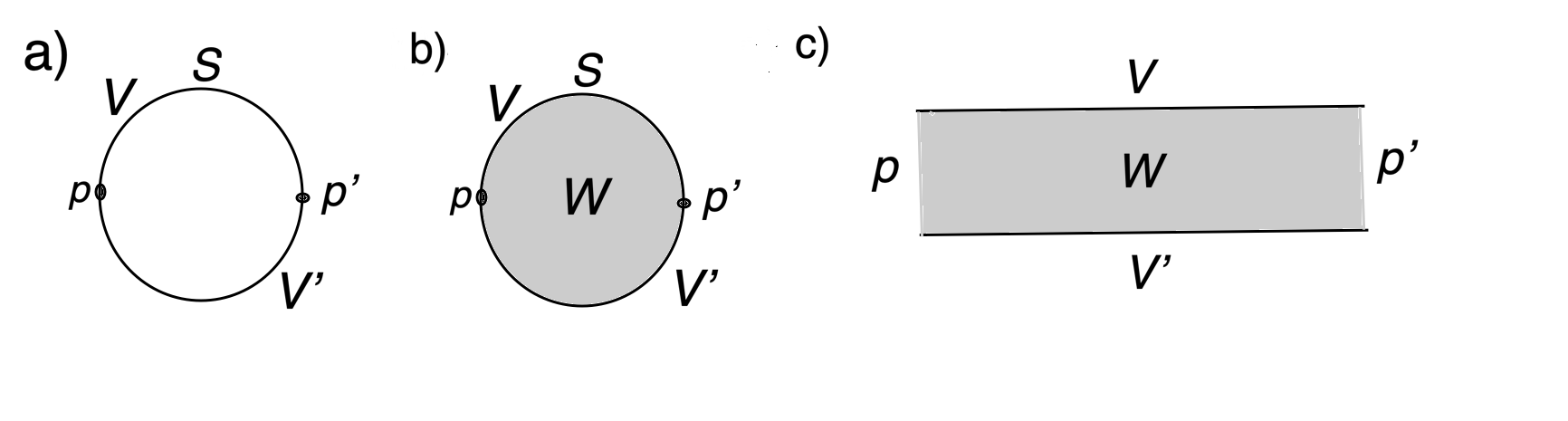
Figure 3: (a) In a two-dimensional spacetime, we consider a Cauchy hypersurface consisting of a circle $S$. The entangling surface $B$ is a pair of points $p,p^{\prime}$, whose complement in $S$ consists of the two intervals $V$ and $V^{\prime}$. (b) A path integral on the disc $W$, whose boundary is $S$, computes the ground state of a conformal field theory. (c) The disc with the points $p$ and $p^{\prime}$ removed can be conformally mapped to ${\mathbb{R}}\times I$, where $I$ is a unit interval. $V$ and $V^{\prime}$ become the two boundary components of ${\mathbb{R}}\times I$, and the points $p,p^{\prime}$ are projected to infinity.

One aspect of the similarity is that in the case of a conformal field theory (CFT), one can actually make a conformal transformation between the two types of divergence. This is best-known in the case of a two-dimensional CFT [41, 42]. One takes the initial value surface $S$ to be a circle, and one takes the entangling surface $B$ to consist of a pair of points $p,p^{\prime}\in S$; the complement of these points is the union of two open intervals $V$ and $V^{\prime}$ (fig. 3(a)). Let ${\mathcal{H}}$ be the Hilbert space of the given theory formulated on $S$. The conformally invariant ground state $\Omega\in{\mathcal{H}}$ can be computed by a path integral on a disc $W$ whose boundary is $S$ (fig. 3(b)). The state $\Omega$ is highly entangled between regions $V$ and $V^{\prime}$. If one tries to quantify this entanglement by computing the entanglement entropy between $V$ and $V^{\prime}$, one runs into an ultraviolet divergence which is related to the fact that the local algebras actually are of Type III. This ultraviolet divergence can be converted into an infrared divergence by a conformal mapping that maps the disc $W$, minus the two points $p$ and $p^{\prime}$, to an infinite strip ${\mathbb{R}}\times I$, where $I$ is an interval (fig. 3(c)). After a Weyl rescaling, one can take the metric of ${\mathbb{R}}\times I$ to be the flat metric ${\mathrm{d}}x^{2}+{\mathrm{d}}\tau^{2}$, $-\infty<x<\infty$, $0\leq\tau\leq 1$. The path integral on this strip describes the thermofield double of the theory under study on the noncompact initial value surface $S^{\prime}={\mathbb{R}}$, and with inverse temperature 1; the two open intervals $V$ and $V^{\prime}$ have become the boundaries of the strip at $\tau=0,1$, corresponding to the two copies in the thermofield double. The points $p$ and $p^{\prime}$ have been projected to $x=\pm\infty$. In the description on the disc, there is an ultraviolet divergence in the entanglement entropy of the vacuum that arises from the behavior of modes on opposite sides of the points $p$ or $p^{\prime}$. In the description on the strip, this divergence is reinterpreted as an infrared divergence in the entanglement entropy of the thermofield double near $x=\pm\infty$.

All this has an analog for a conformally invariant theory in any dimension $D$ [43, 44]. One takes the initial value surface $S$ to be a $(D-1)$-sphere with a round metric. One further takes the entangling surface $B$ to be an “equator” in $S$, and $V$ and $V^{\prime}$ to be the northern and southern hemispheres. Thus the setup is the same as before, except that $S$ is a $(D-1)$-sphere instead of a circle, and for $D>2$, the equator in $S$ is connected, rather than consisting of two isolated points. The ground state $\Omega$ of a $D$-dimensional CFT can be computed by a path integral on a flat unit ball $W$ in $D$ dimensions, whose boundary is $S$. After removing the equator $B$ of the boundary, $W$ can be conformally mapped to a product $H\times I$, where $H$ is hyperbolic space of dimension $D-1$, and $I$ is again the interval $0\leq\tau\leq 1$. A path integral on $H\times I$ again describes a thermofield double at termperature 1. The only difference from before is that the spatial manifold $H$ on which the thermodynamics is defined is hyperbolic space of dimension $D-1$ rather than Euclidean space. But $H$ has infinite volume just like Euclidean space, and there is an infrared divergence in the entanglement entropy between the two sides of the thermofield double. This divergence matches the ultraviolet divergence between modes on $V$ and modes on $V^{\prime}$ in the original description on the sphere.

3.5 The Hagedorn Temperature

In this section, we return to the Araki-Woods model of a Hamiltonian that is a sum of single-qubit Hamiltonians $H=\sum_{n=1}^{\infty}H_{n}$, with

$$H_{n}=\begin{pmatrix}0&0\cr 0&E_{n}\end{pmatrix}.$$ (3.19)

Now, however, we assume that $\lim_{n\to\infty}E_{n}=+\infty$. We also assume for convenience that the $E_{n}$ are all positive, so that the ground state of the $n^{th}$ qubit is the state $|\negthinspace\uparrow\rangle_{n}=\begin{pmatrix}1\cr 0\end{pmatrix}$. The ground state of the whole system is $|\Omega\rangle_{\uparrow}=\otimes_{n=1}^{\infty}|\negthinspace\uparrow\rangle_{n}$. As in section 2.2, a Hilbert space ${\mathcal{H}}^{*}$ that describes all states of infinitely many qubits is nonseparable. But we can define a separable Hilbert space ${\mathcal{H}}$ in which every state can be approximated by states in which all but finitely many qubits are in their ground state $|\negthinspace\uparrow\rangle_{n}$.

${\mathcal{H}}$ has a basis consisting of states in which all qubits except some finite subset $n_{1},n_{2},\cdots,n_{k}$ are in their ground state. The energy of such a state is $E=E_{n_{1}}+E_{n_{2}}+\cdots+E_{n_{k}}$. Now let us ask this question: What is the probability to observe such a state in a thermal ensemble, at inverse temperature $\beta$? The probability to observe a microstate of energy $E$ is of course $p(E,\beta)=\frac{1}{Z(\beta)}e^{-\beta E}$, where

$$Z(\beta)=\prod_{n=1}^{\infty}(1+e^{-\beta E_{n}})$$ (3.20)

is the partition function. In section 3.1, we studied models in which the partition function diverges in the limit of infinitely many qubits, but now we wish to consider the case that the $E_{n}$ tend to infinity quickly enough that $Z(\beta)$ converges, at least for some range of $\beta$. Clearly when $Z(\beta)<\infty$, we have $p(E,\beta)>0$ and the probability to observe any given microstate in ${\mathcal{H}}$ in the thermal ensemble is positive.

This suggests that the thermal ensemble at inverse temperature $\beta$ can simply be defined in the Hilbert space ${\mathcal{H}}$. To see that this is the case, let us ask what is the probability that, for some $N$, all qubits except the first $N$ are in their ground state. The probability for this in the thermal ensemble is $Z_{N}(\beta)/Z(\beta)$, where $Z_{N}(\beta)$ is a truncated partition function defined for the first $N$ qubits:

$$Z_{N}(\beta)=\prod_{n=1}^{N}(1+e^{-\beta E_{n}}).$$ (3.21)

If $Z(\beta)=\infty$, then $Z_{N}(\beta)/Z(\beta)=0$ for all $N$, since $Z_{N}(\beta)$ is finite, but if $Z(\beta)<\infty$, then

$$\lim_{N\to\infty}\frac{Z_{N}(\beta)}{Z(\beta)}=1.$$ (3.22)

For $Z(\beta)<\infty$, this shows that, with probability 1, any state in the thermal ensemble can be approximated arbitrarily well by states in ${\mathcal{H}}$.

Therefore, in this situation, it is not necessary to go to the thermofield double in order to describe the thermal ensemble of an infinite number of qubits in a separable Hilbert space. What happens if we do go to the thermofield double anyway? The answer is that we get nothing essentially new; when $Z<\infty$ the thermofield double does not combine the two copies in an interesting way.

To explain how this comes about, we consider two copies of this system, the left and right copy, each consisting of countably many qubits with identical Hamiltonians. There are nonseparable Hilbert spaces ${\mathcal{H}}_{\ell}^{*}$ and ${\mathcal{H}}_{r}^{*}$ that describe all possible states of the left and right systems, and these contain separable subspaces ${\mathcal{H}}_{\ell}$ and ${\mathcal{H}}_{r}$ that have bases with finitely many qubits excited. We also write ${\mathscr{A}}_{\ell,0}$ or ${\mathscr{A}}_{r,0}$ for the algebras of operators that act on finitely many qubits of the left or right systems, respectively, and $\Omega_{\uparrow,r}$, $\Omega_{\uparrow,\ell}$ for the ground states of the right and left systems.

We can define the thermofield double state in the naive way as a vector in ${\mathcal{H}}_{\ell}^{*}\otimes{\mathcal{H}}_{r}^{*}$:

$$\Psi_{\mathrm{TFD}}=\frac{1}{\sqrt{Z(\beta)}}\bigotimes_{n=1}^{\infty}\begin{pmatrix}1&0\cr 0&e^{-\beta E_{n}/2}\end{pmatrix}.$$ (3.23)

Then we define the thermofield double Hilbert space ${\mathcal{H}}_{\mathrm{TFD}}$ as the closure of the set of all vectors of the form ${\sf a}_{r}\Psi_{\mathrm{TFD}}$, ${\sf a}_{r}\in{\mathscr{A}}_{r,0}$.

In section 3.3, we could not define the thermofield double state and Hilbert space of an infinite system in this simple way, because we were considering systems with $Z(\beta)=\infty$. Therefore, in eqns. (3.14) and (3.17), we defined the thermofield double state directly by a formula analogous to (3.23) for a finite system of $N$ qubit pairs, and we invoked the GNS construction to define $\Psi_{\mathrm{TFD}}$ and ${\mathcal{H}}_{\mathrm{TFD}}$ in the limit of an infinite system.

A priori, eqn. (3.23) defines $\Psi_{\mathrm{TFD}}$ as a vector in the nonseparable Hilbert space ${\mathcal{H}}_{\ell}^{*}\otimes{\mathcal{H}}_{r}^{*}$, and likewise it defines ${\mathcal{H}}_{\mathrm{TFD}}$ as a subspace of that space. But actually, when $Z(\beta)<\infty$ so that the definition (3.23) makes sense, ${\mathcal{H}}_{\mathrm{TFD}}$ is the same as the separable Hilbert space ${\mathcal{H}}_{\ell}\otimes{\mathcal{H}}_{r}$. To see this, observe that a truncated version of $\Psi_{\mathrm{TFD}}$, namely

$$\Psi_{{\mathrm{TFD}},N}=\frac{1}{\sqrt{Z(\beta)}}\bigotimes_{n=1}^{N}\begin{pmatrix}1&0\cr 0&e^{-\beta E_{n}/2}\end{pmatrix}\bigotimes_{n=N+1}^{\infty}\begin{pmatrix}1&0\cr 0&0\end{pmatrix}$$ (3.24)

is manifestly contained in ${\mathcal{H}}_{\ell}\otimes{\mathcal{H}}_{r}$. But $\lim_{N\to\infty}\Psi_{{\mathrm{TFD}},N}=\Psi_{{\mathrm{TFD}}}$. So $\Psi_{{\mathrm{TFD}}}\subset{\mathcal{H}}_{\ell}\otimes{\mathcal{H}}_{r}$. This implies that ${\mathcal{H}}_{\mathrm{TFD}}\subset{\mathcal{H}}_{\ell}\otimes{\mathcal{H}}_{r}$, since ${\mathcal{H}}_{\mathrm{TFD}}$ is generated from $\Psi_{\mathrm{TFD}}$ by the action of ${\mathscr{A}}_{r,0}$, and ${\mathcal{H}}_{\ell}\otimes{\mathcal{H}}_{r}$ is closed under the action of ${\mathscr{A}}_{r,0}$. Conversely, ${\mathscr{A}}_{r,0}$ contains an operator $\Pi_{N}$ that projects onto the ground state of the first $N$ qubits, and acts trivially on others; since $|\Omega\rangle_{\uparrow,\ell}\otimes|\Omega\rangle_{\uparrow,r}=Z(\beta)\lim_{N\to\infty}\Pi_{N}\Psi_{\mathrm{TFD}}$, we have $|\Omega\rangle_{\uparrow,\ell}\otimes|\Omega\rangle_{\uparrow,r}\in{\mathcal{H}}_{\mathrm{TFD}}$, implying, since ${\mathcal{H}}_{\ell}\otimes{\mathcal{H}}_{r}$ is generated from $|\Omega\rangle_{\uparrow,\ell}\otimes|\Omega\rangle_{\uparrow,r}$ by acting with ${\mathscr{A}}_{\ell,0}\otimes{\mathscr{A}}_{r,0}$, that ${\mathcal{H}}_{\ell}\otimes{\mathcal{H}}_{r}\subset{\mathcal{H}}_{\mathrm{TFD}}$.

In short, when $Z(\beta)<\infty$, the thermofield double Hilbert space ${\mathcal{H}}_{\mathrm{TFD}}$ is just a simple tensor product ${\mathcal{H}}_{\mathrm{TFD}}={\mathcal{H}}_{\ell}\otimes{\mathcal{H}}_{r}$. Likewise, if we take the closures of ${\mathscr{A}}_{\ell,0}$ and ${\mathscr{A}}_{r,0}$ to get von Neumann algebras ${\mathscr{A}}_{\ell}$ and ${\mathscr{A}}_{r}$ that act on the thermofield double, we get nothing essentially new: ${\mathscr{A}}_{\ell}$ and ${\mathscr{A}}_{r}$ are simply the Type I_∞ algebras of all bounded operators on ${\mathcal{H}}_{\ell}$ and ${\mathcal{H}}_{r}$, respectively. In this situation, the Hamiltonians $H_{\ell}$ and $H_{r}$ of the left and right systems are well-defined as operators on ${\mathcal{H}}_{\mathrm{TFD}}$ and are elements of ${\mathscr{A}}_{\ell}$ and ${\mathscr{A}}_{r}$ respectively. All in all, when $Z(\beta)<\infty$, we gain little by going to the thermofield double; it is just a tensor product of two decoupled systems.

On the other hand, if $Z(\beta)=\infty$, we are in the situation described in section 3.3. The thermofield double Hilbert space ${\mathcal{H}}_{\mathrm{TFD}}$ is an essentially new construction, not a simple tensor product, and the corresponding algebras ${\mathscr{A}}_{\ell}$ and ${\mathscr{A}}_{r}$ are generically of Type III₁. The operators $H_{\ell}$ and $H_{r}$ cannot be defined as operators on ${\mathcal{H}}_{\mathrm{TFD}}$. As a partial substitute one has $\widehat{H}=H_{r}-H_{\ell}$, which does have a limit for the infinite system, and generates a group of outer automorphisms of ${\mathscr{A}}_{r}$ and of ${\mathscr{A}}_{\ell}$.

A particularly interesting case, and important background for section 4, is the borderline case in which $Z(\beta)<\infty$ at low enough temperature, but $Z(\beta)=\infty$ at sufficiently high temperature. This can happen if $E_{n}\sim c\log n$ for large $n$, with a constant $c$. Then at low temperatures, the thermofield double construction just describes two decoupled systems, and all algebras are of Type I. But at high termperatures, the thermofield double construction is genuinely new, combines the two systems in a subtle way, and is essential if we wish to describe the infinite qubit system in a separable Hilbert space. The algebras are of Type III, and time translations of the algebras are a group of outer automorphisms. By analogy with standard terminology in strong interaction theory, string theory, and large $N$ gauge theory, we call the temperature at which $Z(\beta)$ ceases to converge the Hagedorn temperature $T_{H}$, and we also write $\beta_{H}=1/T_{H}$.

3.6 Density Matrices and Entropy

For a quantum system with a Hilbert space ${\mathcal{H}}$ of physical states, one usually defines the von Neumann entropy, for a state of the system described by a density matrix $\rho:{\mathcal{H}}\to{\mathcal{H}}$, by $S(\rho)=-{\rm Tr}\,\rho\log\rho$. As usual, here $\rho$ is a positive self-adjoint operator normalized to ${\rm Tr}\,\rho=1$. The trace function ${\sf a}\to{\rm Tr}\,{\sf a}$ is a complex linear function from the algebra ${\mathscr{A}}$ of all operators on ${\mathcal{H}}$ (or all bounded operators if ${\mathcal{H}}$ is infinite-dimensional) to ${\mathbb{C}}$; it satisfies ${\rm Tr}\,{\sf a}^{\dagger}{\sf a}>0$ for all ${\sf a}\not=0$. This last condition ensures that the function $F({\sf a})={\rm Tr}\,{\sf a}\rho$ satisfies the conditions as stated in section 2.5 for a state on the algebra ${\mathscr{A}}$. Conversely, every state on the algebra ${\mathscr{A}}$ is of the form $F({\sf a})={\rm Tr}\,{\sf a}\rho$ for some density matrix $\rho$. To prove this, one first observes that the trace is nondegenerate, in the sense that every linear function on ${\mathscr{A}}$ is of the form $F({\sf a})={\rm Tr}\,{\sf a}{\sf b}$ for some ${\sf b}\in{\mathscr{A}}$. The other axioms for a state (namely $F({\sf a}^{\dagger}{\sf a})\geq 0$ and $F(1)=1$) imply that $\rho$ must be a positive operator satisfying ${\rm Tr}\,\rho=1$, in other words, a density matrix.

Now consider any von Neumann algebra ${\mathscr{A}}$ that acts on a Hilbert space ${\mathcal{H}}$. An element of ${\mathscr{A}}$ is called positive if it corresponds to a positive, self-adjoint operator on ${\mathcal{H}}$. If the algebra ${\mathscr{A}}$ has a nondegenerate trace, then the same arguments as before show that any state on ${\mathscr{A}}$ is of the form $F({\sf a})={\rm Tr}\,{\sf a}\rho$, where $\rho$ is a density matrix, that is, a positive element of ${\mathscr{A}}$ of trace 1. We can then define, for any state, the von Neumann entropy $S(\rho)=-{\rm Tr}\rho\log\rho$. In this article, the von Neumann algebras that we consider are factors, that is, algebras with trivial center (in other words, algebras whose center consists only of ${\mathbb{C}}$). A factor is the von Neumann algebra analog of a simple Lie group. In the case of a factor, any trace is nondegenerate and therefore the condition to be able to define a von Neumann entropy is only that ${\mathscr{A}}$ has a trace. Also, in the case of a factor, if a trace exists, it is unique up to a multiplicative constant. As we will see, in general it is important that the trace is not quite unique.

Let us discuss entropy for the different types of von Neumann algebra. The original arena for von Neumann entropy is a Type I algebra, which acts irreducibly on a Hilbert space ${\mathcal{H}}$. A standard argument shows that $S(\rho)$ is always nonnegative in this case. A subtlety is that in the case of a Type I_∞ algebra, that is, if ${\mathcal{H}}$ is infinite-dimensional, it is possible to have $S(\rho)=+\infty$. That is because the condition ${\rm Tr}\,\rho=1$ does not ensure the convergence of ${\rm Tr}\,\rho\log\rho$. Thus for Type I_∞, the entropy takes values in ${\mathbb{R}}_{\geq 0}\cup+\infty$.

Now let us consider algebras of Type II and Type III. A Type III algebra has no trace and therefore no notion of von Neumann entropy. However, a Type II algebra does have a trace, as explained in section 3.3, and therefore one can define an entropy for a state of a von Neumann algebra of Type II.

Let us explore this notion, initially for the case of Type II₁. We recall that a Type II₁ algebra ${\mathscr{A}}$ has a trace that is defined for all elements of ${\mathscr{A}}$, and is conventionally normalized so that ${\rm Tr}\,1=1$. The simplest density matrix to consider is $\rho=1$. In this case, $\log\rho=0$ so $S(\rho)=-{\rm Tr}\,\rho\log\rho=0$. But what $\rho$ describes is far from being a zero entropy state in any conventional sense. In fact, the density matrix $\rho=1$ describes the maximally entangled thermofield double state $\Psi_{\mathrm{TFD}}$ that was defined in eqn. 3.14. Indeed, we defined the trace in a Type II₁ algebra by ${\rm Tr}\,{\sf a}=\langle\Psi_{\mathrm{TFD}}|{\sf a}|\Psi_{\mathrm{TFD}}\rangle$. This implies that to satisfy ${\rm Tr}\,{\sf a}\rho=\langle\Psi_{\mathrm{TFD}}|{\sf a}|\Psi_{\mathrm{TFD}}\rangle$, we need to take $\rho=1$, so $\rho=1$ is the density matrix that corresponds to the maximally entangled thermofield double state $\Psi_{\mathrm{TFD}}$.

The maximally entangled state of $N$ qubit pairs has von Neumann entropy $N\log 2$, and to get a Type II₁ algebra, one takes the limit $N\to\infty$. So the entropy diverges for $N\to\infty$. But with the Type II₁ definition of entropy, the large $N$ limit of the thermofield double state is deemed to have entropy 0. This suggests that in general Type II₁ entropy is ordinary von Neumann entropy with the entropy of a maximally entangled state subtracted. To confirm this interpretation, recall that a general state of a Type II₁ algebra can be associated to a system of $N$ qubit pairs, in the large $N$ limit, in a state in which almost all the qubit pairs are almost maximally entangled. As an illustrative example, suppose that the first $k$ qubits are definitely in a “spin up” state, and the others are maximally mixed. To describe this state by a density matrix, let $\Pi$ be the orthogonal projection operator onto the subspace of states of $N$ qubits in which the first $k$ qubits all have spin up. For finite $N$, $\rho=2^{-(N-k)}\Pi$ is a density matrix of the $N$ qubit system, and its von Neumann entropy is $S_{N}=(N-k)\log 2$. But in the limit $N\to\infty$, $\Pi$ becomes an element of the Type II₁ algebra with ${\rm Tr}\,\Pi=2^{-k}$. So in the Type II₁ algebra, we can define a density matrix $\rho=2^{k}\Pi$, with ${\rm Tr}\,\rho=1$. For this density matrix, we compute $S=-{\rm Tr}\,\rho\log\rho=-k\log 2$. This is the same as $S=\lim_{N\to\infty}(S_{N}-N\log 2)$. In other words, $S$ is the large $N$ limit of $S_{N}-N\log 2$, or differently put, it is the large $N$ limit of the entropy difference between the actual state of the first $N$ qubits and a maximally mixed state. As this example and discussion suggest, entropy is negative definite for a Type II₁ factor.

A Type III algebra can similarly be constructed, as described in section 3.3, from an infinite collection of (non-maximally) entangled qubit pairs. But in this case, there is no way, using only the structure of the algebra, to define a renormalized entropy. This is reflected in the fact that the divergences in the entanglement entropy of a local region in quantum field theory are model-dependent (there is a leading divergence proportional to the area of the boundary of the region, with a theory-dependent coefficient, and there are subleading divergences that depend on the spacetime dimension and the operator content of the theory). Renormalized entropies of local regions in quantum field theory can be useful and important, but defining them requires information beyond the von Neumann algebra structure. Similar remarks apply in quantum statistical mechanics if one considers the entropy of a state that is not thermal but looks thermal near spatial infinity.

Now let us consider an algebra ${\mathscr{A}}$ of Type II_∞. Such an algebra can be factored as ${\mathscr{A}}={\mathscr{A}}_{1}\otimes{\mathscr{A}}_{2}$, where ${\mathscr{A}}_{1}$ is of Type II₁ and ${\mathscr{A}}_{2}$ is the type I_∞ algebra of bounded operators on a separable Hilbert space ${\mathcal{K}}$. We can define a trace ${\rm Tr}_{1}$ on ${\mathscr{A}}_{1}$ normalized so that ${\rm Tr}_{1}\,1=1$, and a trace ${\rm Tr}_{2}$ on ${\mathscr{A}}_{2}$ normalized so that, if $\Pi\in{\mathscr{A}}_{2}$ is the orthogonal projection operator on a one-dimensional subspace ${\mathcal{K}}_{0}\subset{\mathcal{K}}$, then ${\rm Tr}_{2}\,\Pi=1$. Then we can define a trace on ${\mathscr{A}}$ by ${\rm Tr}={\rm Tr}_{1}\otimes{\rm Tr}_{2}$.

Since a trace is available, there is a notion of entropy for such an algebra ${\mathscr{A}}$. But there is a very important subtlety: there is no canonical way to normalize this trace. One immediate observation is that, since the identity element of ${\mathscr{A}}_{2}$ has a divergent trace, we cannot normalize the trace, as we did for Type II₁, by saying that the identity element has trace 1. A deeper explanation involves the fact that a Type II_∞ algebra can be factored as the tensor product of algebras of Type II₁ and Type I_∞ in many different ways.

Let ${\mathscr{A}}_{3}$ be an algebra of Type I_n, acting on an $n$-dimensional Hilbert space ${\mathcal{H}}_{n}$, and define the trace ${\rm Tr}_{3}$ on ${\mathscr{A}}_{3}$ to be the usual trace of a linear transformation acting on ${\mathcal{H}}_{n}$. Thus ${\rm Tr}_{3}\,1=n$. Consider the algebra ${\mathscr{A}}={\mathscr{A}}_{1}\otimes{\mathscr{A}}_{2}\otimes{\mathscr{A}}_{3}$, with ${\mathscr{A}}_{1}$ and ${\mathscr{A}}_{2}$ as before. The algebra ${\mathscr{A}}_{1}^{\prime}={\mathscr{A}}_{1}\otimes{\mathscr{A}}_{3}$ is of Type II₁, and the algebra ${\mathscr{A}}_{2}^{\prime}={\mathscr{A}}_{2}\otimes{\mathscr{A}}_{3}$ is of Type I_∞. So ${\mathscr{A}}={\mathscr{A}}_{1}^{\prime}\otimes{\mathscr{A}}_{2}={\mathscr{A}}_{1}\otimes{\mathscr{A}}_{2}^{\prime}$ gives two different factorizations of the same Type II_∞ factor as the tensor product of factors of Type II₁ and Type I_∞. These two factorizations of ${\mathscr{A}}$ lead to definitions of the trace that differ by a factor of $n$. To see this, consider the element ${\sf a}=1\otimes\Pi\otimes 1\in{\mathscr{A}}_{1}\otimes{\mathscr{A}}_{2}\otimes{\mathscr{A}}_{3}$, where as before $\Pi$ is an element of ${\mathscr{A}}_{2}$ that projects on a one-dimensional subspace ${\mathcal{K}}_{0}\subset{\mathcal{K}}$. With respect to the factorization of ${\mathscr{A}}$ as ${\mathscr{A}}_{1}^{\prime}\otimes{\mathscr{A}}_{2}$, ${\sf a}$ is the tensor product of $1\in{\mathscr{A}}_{1}^{\prime}$ with $\Pi\in{\mathscr{A}}_{2}$, so the normalization of the trace that is natural for this factorization gives ${\rm Tr}\,{\sf a}={\rm Tr}\,1\otimes\Pi=1$. On the other hand, with respect to the factorization of ${\mathscr{A}}$ as ${\mathscr{A}}_{1}\otimes{\mathscr{A}}_{2}^{\prime}$, ${\sf a}$ is $1\otimes\Pi^{\prime}$, where $\Pi^{\prime}$ projects on the $n$-dimensional subspace ${\mathcal{K}}_{0}\otimes{\mathcal{H}}_{n}\subset{\mathcal{K}}\otimes{\mathcal{H}}_{n}$. So with the normalization of the trace that is natural for this second factorization, we would have ${\rm Tr}\,{\sf a}=n$.

Thus different choices of factorization motivate different normalizations of the trace for a Type II_∞ factor. In fact, there can be no natural normalization of the trace, because a Type II_∞ algebra has an outer automorphism group that rescales the trace by any positive real number. (This is a standard result in von Neumann algebra theory and will be explained elsewhere [23].) However, as long as we assume our algebra to be a factor, analogous to a simple Lie group, the only indeterminacy in the trace is an overall multiplicative constant.

Let us see how this indeterminacy affects the definition of entropy. If we rescale the trace by ${\rm Tr}\to\lambda{\rm Tr}$, we must compensate by rescaling the density matrix by $\rho\to\lambda^{-1}\rho$, to preserve ${\rm Tr}\,\rho=1$. Under the combined rescaling of ${\rm Tr}$ and $\rho$, we have

$$S(\rho)=-{\rm Tr}\,\rho\log\rho\to S(\rho)+\log\lambda.$$ (3.25)

In other words, when we rescale the trace by a factor $\lambda$, the entropy of any state is shifted by an additive constant $\log\lambda$, independent of the state.

This means that entropy in a Type II_∞ factor is somewhat analogous to entropy in classical mechanics. The concept of entropy was originally discovered in the 19th century by macroscopic arguments, which showed that there must be a state function $S$ of a system in thermal equilibrium that obeys the first law of thermodynamics. If the relevant thermodynamic variables are the energy $E$, temperature $T$, pressure $p$, and volume $V$, then the first law reads

$${\mathrm{d}}E=T{\mathrm{d}}S-p{\mathrm{d}}V.$$ (3.26)

This equation determines $S$ up to an additive constant. Quantum mechanically, one can fix the additive constant by saying that (assuming the system under study has a unique ground state) the entropy vanishes at $T=0$. Classically, no such statement is possible, because for example the entropy of a classical harmonic oscillator goes to $-\infty$ for $T\to 0$.

For another explanation of why it is difficult in classical physics to fix an overall additive constant in the entropy, consider a system of particles with positions $\vec{x}$ and momenta $\vec{p}$. One can describe one’s state of knowledge about the system with a probability distribution function $\rho(\vec{p},\vec{x})$. Then a classical definition of entropy is

$$S=-\int{\mathrm{d}}\vec{p}\,{\mathrm{d}}\vec{x}\rho(\vec{p},\vec{x})\log\rho(\vec{p},\vec{x}).$$ (3.27)

The integral runs over the classical phase space of the system. But classically, there is no natural way to normalize the phase space measure, since, for any pair of canonical variables $p,x$, the measure ${\mathrm{d}}p\,{\mathrm{d}}x$ has dimensions of action, and classically there is no natural constant with dimensions of action that could be used to normalize it. (Quantum mechanically, one replaces ${\mathrm{d}}p\,{\mathrm{d}}x$ by ${\mathrm{d}}p\,{\mathrm{d}}x/2\pi\hbar$.) The phase space measure in classical mechanics is naturally defined up to an overall multiplicative constant, but there is no natural way to fix this constant. If we rescale the measure by ${\mathrm{d}}\vec{p}\,{\mathrm{d}}\vec{x}\to\lambda{\mathrm{d}}\vec{p}\,{\mathrm{d}}\vec{x}$, for a positive constant $\lambda$, then we have to compensate by $\rho\to\lambda^{-1}\rho$. But this then shifts $S$ by $S\to S+\log\lambda$, just as in the discussion of a Type II_∞ algebra.

Here is an interesting example of entropy for a state of a Type II_∞ algebra ${\mathscr{A}}$. Pick a factorization ${\mathscr{A}}={\mathscr{A}}_{1}\otimes{\mathscr{A}}_{2}$ where ${\mathscr{A}}_{1}$ is of Type II₁ and ${\mathscr{A}}_{2}$ is of Type I_∞. Let $\Pi_{k},$ $k=1,\cdots,n$, be orthogonal projection operators in ${\mathscr{A}}_{1}$ satisfying $\Pi_{i}\Pi_{j}=\delta_{ij}\Pi_{j}$, ${\rm Tr}\,\Pi_{i}=p_{i}$, $\sum_{k=1}^{n}\Pi_{k}=1$. Let $\rho_{k}$, $k=1,\cdots,n$ be any density matrices in ${\mathscr{A}}_{2}$. Then $\rho=\sum_{k=1}^{n}\Pi_{k}\otimes\rho_{k}$ is a density matrix in ${\mathscr{A}}$. Its entropy is

$$S(\rho)=\sum_{k}p_{k}S(\rho_{k})=-\sum_{k}p_{k}{\rm Tr}\,\rho_{k}\log\rho_{k}.$$ (3.28)

In verifying this, one uses the fact that $\Pi_{k}\log\Pi_{k}=0$ for all $k$, since the only eigenvalues of $\Pi_{k}$ are 0 and 1, and $x\log x=0$ if $x=0$ or 1. It is noteworthy that in the formula for $S(\rho)$ there is no Shannon term $-\sum_{k}p_{k}\log p_{k}$. Thus in this particular example, Type II_∞ entropy is the average entropy of an ensemble of density matrices.

We have phrased this discussion in terms of the von Neumann entropy, but similar remarks apply for other information theoretic measures such as the Renyi entropies $S_{\alpha}(\rho)=\frac{1}{1-\alpha}\log{\rm Tr}\,\rho^{\alpha}$. These entropies can be defined for a state on an algebra of Type I or Type II (but not, of course, Type III). In the Type II_∞ case, if we rescale the trace by a factor $\lambda$ and compensate by rescaling the density matrix $\rho\to\lambda^{-1}\rho$, the Renyi entropies are shifted by

$$S_{\alpha}(\rho)\to S_{\alpha}(\rho)+\frac{\alpha}{\alpha-1}\log\lambda.$$ (3.29)

Thus all the Renyi entropies are well-defined in Type II_∞, up to a shift that is controlled in this way by the same $\alpha$-independent parameter $\lambda$ that controls the indeterminacy in the von Neumann entropy.

4 The Large $N$ Limit and the Thermofield Double

QCD in Minkowski space is confining at low temperatures and has a deconfinement transition at a certain positive temperature [47, 48, 49]. In finite volume, this transition is smoothed out. But if we replace QCD, which has gauge group $SU(3)$, with a theory with gauge group $SU(N)$ (or $SO(N)$ or $Sp(N)$), then it is believed that in the large $N$ limit, there is a sharp deconfinement transition even in finite volume. This is true even for zero [50, 51, 52, 53] or small [54] coupling. In the case of a gauge theory that has a gravitational dual, this phenomenon is relevant to the AdS/CFT correspondence. In that application, if the bulk spacetime has $D$ noncompact dimensions, so that the conformal boundary has dimension $D-1$, the spatial manifold on which the gauge theory lives is most simply taken to be a sphere ${\sf S}^{D-2}$. Then the deconfinement transition is dual to the Hawking-Page transition [55] between a thermal gas in Anti de Sitter space and a black hole [56]. We call the temperature at which this transition occurs $T_{{H\negthinspace P}}$.

Let ${\mathcal{H}}_{N}$ be the Hilbert space of a large $N$ gauge theory, quantized on the compact manifold ${\sf S}^{D-2}$. It is believed that ${\mathcal{H}}_{N}$ has a large $N$ limit ${\mathcal{H}}_{\infty}$: the energy eigenvalues and multiplicities and the matrix elements of operators all have limits for $N\to\infty$ (and in particular the multiplicities do not grow with $N$). At sufficiently low temperatures, the thermal ensemble can be understood in the limiting Hilbert space ${\mathcal{H}}_{\infty}$. Because the energy eigenvalues and multiplicities have limits for $N\to\infty$, the thermodynamic functions such as entropy, energy, etc., all have large $N$ limits at sufficiently low temperatures. Thus in the low temperature phase, the energy and entropy are of order $N^{0}$ for large $N$. In the range of temperatures at which the thermodynamics can be described in ${\mathcal{H}}_{\infty}$, the natural algebra of observables at large $N$ is simply the Type I_∞ algebra of all operators on ${\mathcal{H}}_{\infty}$.

It is believed that in large $N$ gauge theories, the partition function ${\rm Tr}_{{\mathcal{H}}_{\infty}}\,e^{-\beta H}$, computed in the limiting large $N$ Hilbert space ${\mathcal{H}}_{\infty}$, diverges at a temperature $T_{H}$, known as the Hagedorn temperature. This can be seen quite explicitly at zero coupling. At or below $T_{H}$, the description based on the Hilbert space ${\mathcal{H}}_{\infty}$ has to break down. We will loosely call the transition at which this happens the Hagedorn transition. In various weakly coupled gauge theories, it is believed that the transition occurs at a temperature slightly below $T_{H}$ [54]. In gauge theories – such as ${\mathcal{N}}=4$ super Yang-Mills theory in four dimensions – that participate in AdS/CFT duality, the transition away from a description in the Hilbert space ${\mathcal{H}}_{\infty}$ occurs at the Hawking-Page temperature $T_{{H\negthinspace P}}$, which is far below $T_{H}$ (assuming that $g^{2}N$ is large and the AdS theory can be studied semiclassically). In fact, $T_{H}$ is at the string scale, while $T_{{H\negthinspace P}}$ is of order the inverse radius of the AdS space. Thus in the AdS/CFT context, what we are calling the Hagedorn transition is the same as the Hawking-Page transition and occurs at a temperature far below $T_{H}$. Regardless, above this transition the physics can no longer be described in ${\mathcal{H}}_{\infty}$.

Above the transition temperature, the energy and entropy are both proportional to $N^{2}$ for large $N$ [57] and in particular do not have large $N$ limits. To reach the high temperature phase in the large $N$ limit, we have to take $N\to\infty$ with the energy $E$ proportional to $N^{2}$ (as opposed to taking $N\to\infty$ with fixed $E$, which will always lead to a description in the Hilbert space ${\mathcal{H}}_{\infty}$, regardless of $E$). In brief, we will refer to the large $N$ limit in that regime as the large $N$ limit above the Hagedorn transition. It seems very unlikely that there is a limiting large $N$ Hilbert space that describes the large $N$ limit above the Hagedorn transition. Certainly the literature does not contain any proposal for what such a large $N$ Hilbert space would be. Since the entropy above the Hagedorn transition is of order $N^{2}$, when one increases the rank of the gauge group from $N$ to $N+1$, the entropy increases by a multiple of $N$, and the Hilbert space becomes much bigger. So most “above the Hagedorn transition” microstates with gauge group $SU(N+1)$ are “new” and have no antecedents in the $SU(N)$ theory.

The non-existence of a large $N$ limit of the Hilbert space above the Hagedorn transition would be analogous to the non-existence, in quantum statistical mechanics at temperature $T>0$, of a Hilbert space that describes the infinite volume limit. In this analogy, $N^{2}$ plays the role of the volume $V$. There is also an analogy with the non-existence of a natural Hilbert space description of quantum field theory in an open universe.

The analogy with statistical mechanics also suggests a partial cure, which is to go to the thermofield double. This is particularly powerful in gauge theories that participate in AdS/CFT duality. In such a case, the large $N$ limit of the thermofield double, in the high temperature phase, is a two-sided eternal black hole [58]. By quantizing the low energy bulk fields in the black hole spacetime, one constructs a Hilbert space ${\mathcal{H}}_{\mathrm{TFD}}$. This Hilbert space describes the large $N$ limit of the thermofield double of the gauge theory, in the high temperature phase.

A natural algebra of observables in the large $N$ limit is the algebra of polynomial functions of single trace operators. Based on the analogy with quantum statistical mechanics and the discussion in section 3.5, we can make a guess about the nature of this large $N$ algebra. As already noted, below the Hagedorn transition, the physics can be described in the original large $N$ Hilbert space ${\mathcal{H}}_{\infty}$, and the natural algebra acting on this Hilbert space is of Type I. In the high termperature phase, the analogy with statistical mechanics suggests that the natural algebra of single trace operators would be of Type III. Indeed, this has been argued recently by Leutheusser and Liu [22], who made this claim partly based on the AdS/CFT duality, in a paper with several novel ideas about quantum black holes. These issues and some subtle corrections to the large $N$ limit will be further discussed elsewhere [23].

Finally let us consider the Hamiltonians $H_{r}$ and $H_{\ell}$ that act on the two copies in the thermofield double. What happens in the large $N$ limit above the Hagedorn transition is similar to what happens in the more familiar infinite volume limit. The difference $\widehat{H}=H_{r}-H_{\ell}$ annihilates the thermofield double state $\Psi_{\mathrm{TFD}}$ and converges, in the large $N$ limit, to an operator that acts on the thermofield double Hilbert space ${\mathcal{H}}_{\mathrm{TFD}}$. However, because of fluctuations, $H_{r}$ and $H_{\ell}$ do not separately have large $N$ limits at $\beta<1/T_{{H\negthinspace P}}$. For example, $H_{r}$ has an expectation value $\langle H_{r}\rangle_{\beta}\sim N^{2}$ and so does not have a large $N$ limit. We can of course subtract this expectation value, but the subtracted operator $H_{r}-\langle H_{r}\rangle_{\beta}$ has divergent thermal fluctuations $\left\langle\left(H_{r}-\langle H_{r}\rangle_{\beta}\right)^{2}\right\rangle_{\beta}\sim N^{2}$ and therefore also does not converge for large $N$ to an operator on ${\mathcal{H}}_{\mathrm{TFD}}$. $\widehat{H}$ generates a group of outer automorphisms of the large $N$ operator algebras of the left and right systems. This is a group of outer automorphisms because $H_{\ell}$ and $H_{r}$ do not separately have large $N$ limits.

Acknowledgments I thank H. Liu, R. Longo, R. Mahajan, J. Maldacena, N. Seiberg, J. Turiaci, and R. Wald for helpful and informative discussions. Research supported in part by NSF Grant PHY-1911298.

References

- [1] B. S. DeWitt, “Quantum Field Theory In Curved Spacetime,” Phys. Reports 19 (1975) 295-357.
- [2] S. A. Fulling, M. Sweeny, and R. M. Wald, “Singularity Structure of the Two-Point Function in Quantum Field Theory in Curved Spacetime,” Commun. Math. Phys. 63 (1978) 257-64.
- [3] S. A. Fulling, F. J. Narcowich, and R. M. Wald, “Singularity Structure of the Two-Point Function in Quantum Field Theory in Curved Spacetime, II,” Ann. Phys. 136 (1981) 243-72.
- [4] N. D. Birrell and P. C. W. Davies, Quantum Fields In Curved Space (Cambridge University Press, 1982).
- [5] S. A. Fulling, Aspects of Quantum Field Theory In Curved Spacetime (Cambridge University Press, 1989).
- [6] B. S. Kay, “The Principle Of Locality and Quantum Field Theory on (Non Globally Hyperbolic) Curved Spacetimes,” Rev. Math. Phys. 4 (1992) 167-95.
- [7] I. L. Buchbinder, S. D. Odintsov, and I. L. Shapiro, Effective Action in Quantum Gravity (Taylor&Francis, 1992).
- [8] R. M. Wald, Quantum Field Theory In Curved Spacetime and Black Hole Thermodynamics (University of Chicago, 1994).
- [9] R. Brunetti, K. Fredenhagen, and R. Verch, “The Generally Covariant Locality Principle - A New Paradigm for Local Quantum Field Theory,” arXiv:math-ph/0112041.
- [10] K. Fredenhagen, “Locally Covariant Quantum Field Theory,” arXiv:hep-th/0403007.
- [11] S. Hollands and R. M. Wald, “Axiomatic Quantum Field Theory In Curved Spacetime,” arXiv:0803.2003.
- [12] C. Bar and K. Fredenhagen, eds., Quantum Field Theory On Curved Spacetimes (Springer, 2009).
- [13] L. Parker and D. Toms, Quantum Field Theory In Curved Spacetime (Cambridge University Press, 2009).
- [14] C. J. Fewster, “Locally Covariant Quantum Field Theory and the Problem of Formulating the Same Physics in All Spacetimes,” Phil. Trans. R. Soc. A373 (2015) 20140238, arXiv:1502.04642.
- [15] H. Araki, “Type of von Neumann Algebra Associated with Free Field,” Prog. Theor. Phys. 5 (1964) 1-13.
- [16] K. Fredenhagen, “On The Modular Structure Of Local Algebras Of Observables,” Commun. Math. Phys. 97 (1985) 79.
- [17] R. Haag, Local Quantum Physics (Springer-Verlag, 1992).
- [18] J. Yngvason, “The Role of Type III Factors in Quantum Field Theory,” arXiv:math-ph/0411058.
- [19] E. Witten, “Some Entanglement Properties of Quantum Field Theory,” Rev. Mod. Phys. 90 (2018) 045003, arXiv:1803.04993.
- [20] R. Haag, N. M. Hugenholtz, and M. Winnink, “On The Equilibrium States in Quantum Statistical Mechanics,” Commun. Math. Phys. 5 (1967) 215-236.
- [21] E. Witten, “Quantum Field Theory In Curved Spacetime,” lecture available at https://www.youtube.com/watch?v=8Wu4QhlznnY&t.
- [22] S. Leutheusser and H. Liu, “Causal Connectability Between Quantum Systems and The Black Hole Interior in Holographic Duality,” arXiv:2110.05497.
- [23] E. Witten, “Gravity and the Crossed Product,” to appear.
- [24] M. Kontsevich and G. B. Segal, “Wick Rotation and the Positivity of Energy in Quantum Field Theory,” Quart. J. Math. 72 (2021) 673-99, arXiv:2105.10161.
- [25] J. von Neumann, “Die Eindeutigkeit der Schrödingerschen Operatoren,” Math. Ann. 104 (1931) 570-8.
- [26] L. Gårding and A. Wightman, “Representations of the Commutation Relations,” Proc. NAS 40 (1954) 622-6.
- [27] G. L. Sewell, Quantum Mechanics and its Emergent Macrophysics (Princeton University Press, 2002).
- [28] H. Bostelmann, “Operator Product Expansions As A Consequence Of Phase Space Properties,” arXiv:math-ph/0502004.
- [29] A. Ashtekar, Asymptotic Quantization (Bibliopolis, 1987).
- [30] A. Strominger, Lectures On The Infrared Structure Of Gravity and Gauge Theory (Princeton University Press, 2018).
- [31] K. Prabhu, G. Satishchandran and R. Wald, to appear.
- [32] R. Brunetti and K. Fredenhagen, “Microlocal Analysis and Interacting Quantum Field Theories: Renormalization on Physical Backgrounds,” Commun. Math. Phys. 208 (2000) 623.
- [33] S. Hollands and R. M. Wald, “Existence of Local Covariant Time Ordered Products of Quantum Fields in Curved Spacetime,” gr-qc/0111108.
- [34] J. von Neumann, “On Infinite Direct Products,” Comp. Math. 6 (1938) 1-77.
- [35] R. T. Powers, “Representations of Uniformly Hyperfinite Algebras and Their Associated von Neumann Rings,” Ann. of Math. 86 (1967) 138-171.
- [36] H. Araki and E. J. Woods, “A Classification of Factors,” Publ. RIMS Kyoto Univ. Ser. A 3 (1968) 51-130.
- [37] F. J. Murray and J. von Neumann, “On Rings Of Operators,” Ann. Math. 37 (1936) 116-229.
- [38] W. G. Unruh, “Notes On Black Hole Evaporation,” Phys. Rev. D14 (1976) 870-892.
- [39] J. Bisognano and E. H. Wichmann, “On The Duality Condition For Quantum Fields,” J. Math. Phys. 17 (1976) 303-21.
- [40] G. L. Sewell, “Quantum Fields On Manifolds: PCT and Gravitationally Induced Thermal States,” Ann. Phys. 141 (1982) 201-24.
- [41] C. Holzhey, F. Larsen, and F. Wilczek, “Geometric and Renormalized Entropy In Conformal Field Theory,” Nucl. Phys. B300 (1994) 44.
- [42] P. Calabrese and J. Cardy, “Entanglement Entropy and Quantum Field Theory,” J. Stat. Mech. P06002 (2004) arXiv:hep-th/0405152.
- [43] H. Casini and M. Huerta, “Entanglement Entropy For The -Sphere,” Phys. Lett. B694 (2011) 167-71, arXiv:1007.1813.
- [44] H. Casini, M. Huerta, and R. C. Myers, “Towards A Derivation Of Holographic Entanglement Entropy,” JHEP 05 (2011) 036, arXiv:1102.0440.
- [45] I. E. Segal, “A Note On The Concept of Entropy,” J. Math. Mech. 9 (1960) 623-29.
- [46] A. Connes and E. Størmer, “Entropy For Automorphisms Of II1 Von Neumann Algebras,” Acta. Math. 134 (1975) 289-306.
- [47] N. Cabibbo and G. Parisi, “Exponential Hadronic Spectrum And Quark Liberation,” Phys. Lett. B59 (1975) 67-9.
- [48] A. M. Polyakov, “Thermal Properties Of Gauge Fields And Quark Liberation,” Phys. Lett. B72 (1978) 477-480.
- [49] L. Susskind, “Lattice Models of Quark Confinement At High Temperature,” Phys. Rev. D20 (1979) 2610-18.
- [50] B. Sundborg, “The Hagedorn Transition, Deconfinement, and SYM Theory,” Nucl. Phys. B573 (2000) 349, arXiv:hep-th/9908001.
- [51] J. Hallin and D. Persson, “Thermal Phase Transition In Weakly interacting, Large QCD,” Phys. Lett. B429 (1998) 232, arXiv:hep-th/9803224.
- [52] A. M. Polyakov, “Gauge Fields and Space-Time,” Int. J. Mod. Phys. A17S1 (2002) 119.
- [53] O. Aharony, J. Marsano, S. Minwalla, K. Papadodimas, and M. Van Raamsdonk, “The Hagedorn/Deconfinement Phase Transition in Weakly Coupled Large Gauge Theories,” Phys. Rev. D74 (2006) 105012, arXiv:hep-th/0310285.
- [54] O. Aharony, J. Marsano, S. Minwalla, K. Papadodimas, and M. Van Raamsdonk, “A First Order Deconfinement Transition In Yang-Mills Theory on a Small ,” Phys. Rev. D71 (2005) 125018, arXiv:hep-th/0502149.
- [55] S. W. Hawking and D. N. Page, “Thermodynamics of Black Holes in Anti de Sitter Space,” Commun, Math. Phys. 87 (1983) 577-88.
- [56] E. Witten, “Anti de Sitter Space and Holography,” Adv. Theor. Math. Phys.2 (1998) 253-291, arXiv:hep-th/9802150.
- [57] C. Thorn, “Infinite QCD At Finite Temperature: Is There An Ultimate Temperature?” Phys.Lett.B99 (1981) 458.
- [58] J. M. Maldacena, “Eternal Black Holes in Anti de Sitter,” JHEP 04 (2003) 021, arXiv:hep-th/0106112.