Rightsizing Clusters for Time-Limited Tasks

Abstract

Cloud computing has emerged as the dominant platform for application deployment on clusters of computing nodes. In conventional public clouds, designing a suitable initial cluster for a given application workload is important in converging to an appropriate computing foot-print during run-time. In the case of edge or on-premise clouds, cold-start rightsizing the cluster at the time of installation is crucial in avoiding the recurrent capital expenditure. In both these cases, balancing cost-performance trade-off is critical in constructing a cluster of compute nodes for hosting an application with multiple tasks, where each task can demand multiple resources, and the cloud offers nodes with different capacity and cost.

Multidimensional bin-packing algorithms can address this cold-start rightsizing problem, but these assume that every task is always active. In contrast, real-world tasks (e.g. load bursts, batch and dead-lined tasks with time-limits) may be active only during specific time-periods or may have very dynamic load profiles. The cluster cost can be reduced by reusing resources via time sharing and optimal packing. This motivates our generalized problem of cold-start rightsizing for time-limited tasks: given a timeline, time-periods and resource demands for tasks, the objective is to place the tasks on a minimum cost cluster of nodes without violating node capacities at any time instance. We design a baseline two-phase algorithm that performs penalty-based mapping of task to node-type and then, solves each node-type independently. We prove that the algorithm has an approximation ratio of $O(D\cdot\min(m,T))$, where $D,m$ and $T$ are the number of resources, node-types and timeslots, respectively, We then present an improved linear programming based mapping strategy, enhanced further with a cross-node-type filling mechanism. Our experiments on synthetic and real-world cluster traces show significant cost reduction by LP-based mapping compared to the baseline, and the filling mechanism improves further to produce solutions within $20\%$ of (a lower-bound to) the optimal solution.

I Introduction

Cloud computing has emerged as the preferred platform due to its flexibility in planning and provisioning computing clusters with resources for application deployment and scaling. An undersized cluster degrades performance, whereas an oversized cluster causes wastage and drives up cost. Rightsizing addresses this trade-off by constructing an optimal cluster that balances cost and capacity. Rightsizing has been well-studied over a wide spectrum from pre-deployment (cold-start) cluster provisioning to dynamic node provisioning (E.g. [17, 35, 37, 34, 24]).

Cold-start rightsizing is used as an effective technique to boot-strap an initial cluster based on the workload characteristics, for large public clouds. The capacity of these initial clusters are then managed using dynamic provisioning techniques such as auto-scalers [21]. Thus, the cold-start righsizing and dynamic provisioning techniques are complementary in nature.

Cold-start rightsizing also plays an important role in limited-resource settings where vast resource pools might not exist to support dynamic auto-scalers. In such scenarios, cold-start rightsizing could be the most suitable approach to shape the cluster to a given workload without incurring any capital expenses or logistical challenges. Examples of these scenarios include Telco clouds[1] which co-host computing clusters on base-stations and on-premise clouds dedicated to a single organization. In such infrastructure settings, installation cost on 5G base-stations could be $3\times$ [8] higher than the operational expenditure. Similar challenges exist in on-premise clouds and edge-clouds[20, 6, 4] which may not have huge resource pools and sufficient number of intra-organization tenants to enable arbitrary on-demand scaling.

This paper deals with cold-start rightsizing that sizes a cluster at the time of installation based on projected demands of the application(s) to be hosted on it. The aim is to address the cost-performance trade-off by constructing an optimal cluster that balances cost and capacity, for a given workload of tasks.

Cold-start Rightsizing. Consider a workload (set of tasks) consisting of $n$ tasks, where each task demands specific quantities of $D$ resources (e.g CPU cores, memory and disk space). The cloud environment offers $m$ types of compute nodes that differ in terms of cost and capacity on the $D$ resources, and a replica of a given node-type is a node. Both demands and capacities can be conveniently represented as $D$-dimensional vectors. The goal is to purchase a minimum cost cluster of nodes and place each task on a node such that the aggregate demand of tasks placed on any node does not exceed its capacity along any dimension (resource). We denote this problem as Rightsizing As discussed below (Prior Work), rightsizing has been well-studied in the contexts of cloud computing, virtual machine migration and bin packing.

Cold-start Rightsizing for Time-Limited Tasks. While the above formulation targets rightsizing purely based on resource-demands, real-world tasks are additionally characterized by timeline properties on when they run, how long they run and how much resources they consume at any given time.

These timeline characteristics are available as direct inputs for batch applications [29], for instance, batch jobs running at 1:00AM for few hours or a burst in service load during peak hours. Similarly, scheduled tasks with deadlines are encountered in edge  [10, 30]. Examples are applications that sample duty-cycled data-sources [36]; or adapting to platform activity (e.g. advanced sleeps modes of 5G New Radio which exploit stable user activity patterns [2]). Since the tasks are active only within a specific time-interval, resources could be reused by other tasks outside the interval. This time-limiting nature of tasks could be exploited in rightsizing the cluster leading to cost reduction. With the above motivation, we introduce and study the generalized cold-start rightsizing problem for time-limited tasks.

The problem, denoted TL-Rightsizing, starts with a set of tasks (with varying demands) and different nodes-types (with varying capacity and cost) as in Rightsizing. In addition, we assume a timeline divided into $T$ discrete timeslots, say a day divided into $T=24$ hours, and each task has start and end timeslots as an interval $[s,e]$. The objective of TL-Rightsizing is to purchase a minimum cost set of nodes and place the tasks on the nodes such that the aggregate demand of tasks placed on any node does not violate its capacity at any timeslot. Figure 1 illustrates TL-Rightsizing and its benefits over Rightsizing.

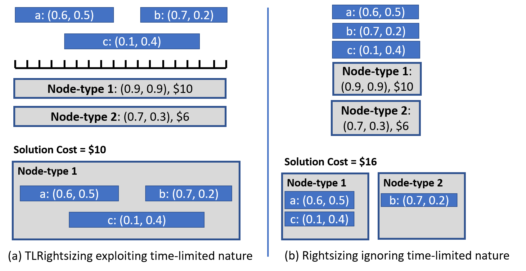
Figure 1: Illustration of TL-Rightsizing. A simple example is shown with two resources ($D=2$), three tasks ($n=3$), and two node-types $(m=2)$. The two dimensional demands and capacities, and node costs are shown. Part (a) shows a solution that exploits the time-limited nature and packs all the tasks in a single node of type 1 with cost $\$10$. In contrast, Part (b) ignores the time-limited aspects, and shows the best solution that packs one node of each type with total cost $\$16$.

For scenarios where demand, start and completion times are not directly known, we could build on cloud-centric time-series analysis  [18, 13] to leverage historical traces of task resource consumption from existing production or test deployments. The resource-demand of the task for various time windows (e.g. hourly, daily, weekly) can be estimated from the traces and each window can be treated as an independent task with a specific start and ending time. For example, a task handling stock market quotes may require high resource regime during market hours and low resource-demand regime at other times. For a timeline that spans a week starting Monday 00:00 hours, we can model this work as six tasks as shown in Figure 2.

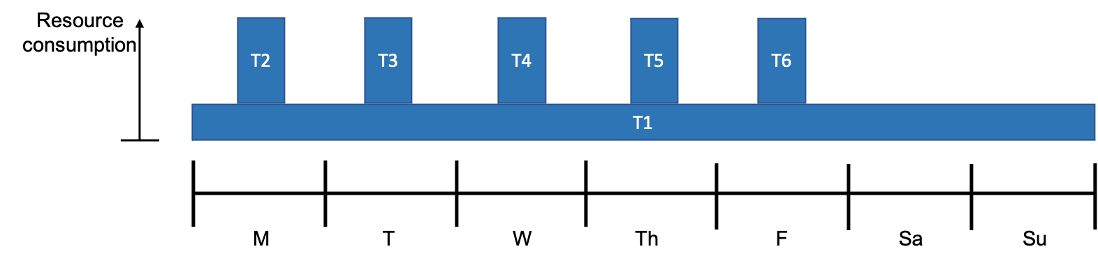
Figure 2: An original long-running task which serves stock market quotes may be modeled as six tasks, spanning a typical week: T1 models the low resource consumption regime, and T2-T6 model the additional demand during the 8-hour high resource consumption regimes during market open hours.

Prior Work. While TL-Rightsizing has not been studied in prior work, two streams of special cases, Rightsizing and interval coloring, have been well explored.

Rightsizing: The Rightsizing problem corresponds to the restricted setting where all the tasks are perpetually active, in other words, there is no consideration of timeline ($T=1$).

If tasks are items and nodes are bins, then the problem corresponds to multi-dimensional bin-packing over multiple bin-types. Since the problem is NP-hard, a polynomial time optimal solution is infeasible, unless NP=P. While exponential time integer programming [15] can produce optimal solutions, meta-heuristics such as genetic algorithms [14], particle swarm [27] and ant colony optimization [11] can handle only small problem sizes due to high running time.

Alternatively, fast and scalable heuristics have been developed by building on strategies from the bin packing domain. Working in the context of optimizing virtual machines, Panigrahy et al. [25] study the single node-type special case ($m=1$), called vector bin packing. They generalize bin packing heuristics (such as first and best-fit) and demonstrate that the heuristics produce near-optimal solutions in practice. Gabay and Zaourar [12] present similar procedures for multiple node-types with uniform costs. Other approaches for special cases and variations of Rightsizing have been proposed (e.g., [16, 22]) and we refer to [28] for a detailed discussion.

We build on the work of Silva et al. [28] and Patt-Shamir and Rawitz [26], who present algorithms for the general Rightsizing problem. The latter work proposes a two-phase procedure that first maps each task to an appropriate node-type by comparing demands and capacities, then solves for each node-type independently. They prove that the algorithm has an approximation ratio of $O(D)$.

From the theoretical perspective, Chekuri and Khanna [7] present an $O(\log D)$-approximation algorithm for the (single node-type) vector bin packing and Patt-Shamir and Rawitz [26] generalize the result to multiple node-types. However, the algorithms are based on an exponential size LP formulation and have a high running time of $n^{O(D)}$.

Interval Coloring (or task scheduling): Interval coloring with bandwidths [3] is equivalent to our setting with single dimensional resources ($D=1$) and single node-type ($m=1$). In this problem, the input is a set of intervals with bandwidth requirements and the objective is to color them with minimum number of colors such that the aggregate bandwidth of intervals of the same color does not exceed a fixed capacity at any timeslot. In our context, the intervals are tasks and the colors are nodes. The problem is studied in both online and offline settings (see survey [19]) and procedures with $O(1)$ approximation ratios have been designed.

Rightsizing for time-limited tasks: The TL-Rightsizing problem generalizes and combines elements from the above two streams: the notion of time-limited tasks from task scheduling, and the concepts of multi-dimensionality and multiple node-types from rightsizing.

Our Contributions. We introduce the TL-Rightsizing problem that reduces the cluster cost by exploiting the time-limited nature of tasks, and make the following contributions:

• We first design a two-phase algorithm, denoted PenaltyMap, that serves as our baseline. The algorithms uses ideas from prior work on Rightsizing and task scheduling. It first maps each task to an appropriate node-type via a penalty-based heuristic and then solves each node-type separately. We present a detailed analysis and prove that the algorithm has an approximation ratio of $O(D\cdot\min(m,T))$.

• While PenaltyMap algorithm performs reasonably well in practice, we identify certain deficiencies in the mapping strategy and develop an improved mapping based on linear programming, denoted LP-map.

• The LP-map algorithm packs tasks mapped to each node-type in a maximal manner, but we observe that it may leave empty capacity that can be filled by tasks mapped to other node-types. We present a cross-node-type filling procedure that reduces the wastage and lowers the overall solution cost.

• We design a scalable strategy (that can handle large inputs) for determining a lowerbound on the optimal cost and use it to measure the efficacy of our algorithms. Using synthetic and real-world traces, we demonstrate that: (i) compared to the baseline PenaltyMap, LP-map offers up to $150\%$ reduction in the cost (normalized with respect to the lowerbound); (ii) cross-node-type filling provides further improvement up to $8\%$, taking the solution closer to the optimal; (iii) the final algorithm (LP-map + cross node-type filling) generates solutions within at most $20\%$ of the lowerbound, and closer in most cases.

II Problem Definition and Modeling

Problem Definition [TL-Rightsizing]. Let the timeline be divided into $T$ discrete timeslots numbered $1,2,\ldots,T$. Let $D$ be the number of resources (or dimensions). We have a set of $m$ node-types ${\cal B}$. Each node-type $B\in{\cal B}$ is associated with a price ${\tt cost}(B)$, and offers a capacity ${\tt cap}(B,d)$, along each dimension $d\in[1,D]$. The input consists of a set of $n$ tasks ${\cal U}$; each task $u\in{\cal U}$ is specified by a demand ${\tt dem}(u,d)$ along each dimension $d$ and a span $[s(u),e(u)]\subseteq[1,T]$, with $s(u)$ and $e(u)$ being the starting and the ending timeslots of $u$. We say that task $u$ is active at a timeslot $t$, if $t\in[s(u),e(u)]$ and denote it as ‘$u\sim t$’.

A $B$-type node refers to a replica $b$ having the same price and capacity: ${\tt cost}(b)={\tt cost}(B)$ and ${\tt cap}(b,d)={\tt cap}(B,d)$, for all $d\in[1,D]$. A feasible solution is to purchase a set of nodes $S$ and place each task in one of the nodes in $S$ such that for any node $b$, the total demand at any timeslot and any dimension does not violate the capacity offered by the node.

$$\forall(t\in[1,T],d\in[1,D]):\sum_{u\sim t~{}\&~{}u\in b}{\tt dem}(u,d)~{}\leq~{}{\tt cap}(b,d),$$

wherein $b$ is viewed as the set of tasks placed in it. We refer to the above as the capacity constraint. A solution may purchase multiple nodes of the same node-type. The cost of the solution is the aggregate cost of the nodes purchased: ${\tt cost}(S)=\sum_{b\in S}{\tt cost}(b)$. The goal is to compute a solution of minimum cost.

Timeline Trimming. While $T$ can be arbitrarily large, as is common in task scheduling (see e.g., [5]), it can trimmed by considering only the start timeslots of tasks and ignoring the rest so that $T\leq n$. It is not difficult to argue that the transformation does not change the set of feasible solutions.

III Penalty-Based Mapping Algorithm

We design a baseline algorithm, denoted PenaltyMap, by building on heuristics from prior work on the following two special cases: interval coloring [17], wherein number of node-types $m=1$ and dimensions $D=1$, and ${\sf Rightsizing}$ [28, 26], wherein there is no timeline ($T=1$).

Two Phase Framework. The intuition behind the algorithm is that each task must be placed on a node whose capacity matches the demand of the task. For instance, placing a task $u$ having high demand along a particular dimension $d$ to a node with low capacity along $d$ would block us from accommodating other tasks on the node, leading to capacity wastage along the other dimensions. The algorithm addresses the issue by using a two-phase framework. First, each task $u\in{\cal U}$ is mapped to a suitable node-type $B$ by comparing the demand of $u$ with the capacities of the node-types. The second phase partitions the tasks based on their node-types and solves each node-type separately, as in the single node-type setting, via a popular heuristic used in interval coloring.

Mapping Phase. For a task $u$, define the relative demand (or height) with respect to a node-type $B$ as:

$$h_{\rm avg}(u|B)=\frac{1}{D}\sum_{d\in[1,D]}\frac{{\tt dem}(u,d)}{{\tt cap}(B,d)}$$

Intuitively, $h_{\rm avg}(u|B)$ is a measure on the space occupied by $u$, if the task were placed in a node of type $B$. Taking the cost into consideration, define the penalty of $u$ relative to $B$ as:

$$p_{\rm avg}(u|B)={\tt cost}(B)\cdot h_{\rm avg}(u|B)$$

We map $u$ to the node-type ${\tt B}^{*}_{\rm avg}(u)$, yielding the least penalty:

$$p^{*}_{\rm avg}(u)=\min_{B\in{\cal B}}~{}p_{\rm avg}(u|B)\mbox{ \& }{\tt B}^{*}_{\rm avg}(u)=\operatorname*{argmin}_{B\in{\cal B}}~{}p_{\rm avg}(u|B)$$

Placement Phase. We partition the tasks based on their node-types and process each group separately. Consider a node-type $B$ and let $V_{B}$ denote the set of tasks mapped to $B$. We process the tasks in $V_{B}$ in the increasing order of starting timeslots. Suppose we have processed a certain number of tasks and have purchased a set of nodes to accommodate them. Let $u$ be the next task. We check if $u$ can fit in some node $b$ purchased already without violating the capacity of the node. If so, among the feasible nodes, we place $u$ in the node purchased the earliest (first-fit). Otherwise, we purchase a new $B$-type node and place $u$ in it. Figure 3 shows a pseudocode.

Alternative Mapping and Fitting Policies. An alternative mapping policy (see [26]) is to define the relative demand as the maximum over the dimensions (as against average), and define the penalty and best node-type analogously:

$$h_{\rm max}(u|B)=\max_{d\in[1,D]}\frac{{\tt dem}(u,d)}{{\tt cap}(B,d)}.$$

An alternative to the first-fit policy is the more refined similarity-fit that emulates the best-fit strategy (adapted from a dot-product strategy [25, 12]). It tries to minimize the capacity wastage by selecting the node $b$ (among the feasible nodes) whose remaining capacity is most similar (dot-product shown below) to the demand of $u$.

$$\sum_{t\in[s(u),e(u)]}\sum_{d}\frac{{\tt dem}(u,d)}{{\tt cap}(B,d)}\times\frac{{\tt rem}(b,d|t)}{{\tt cap}(B,d)},$$

where ${\tt rem}(b,d|t)$ is the remaining capacity of $b$ along dimension $d$ at timeslot $t$. We can derive cosine similarity via dividing the product by the norms of capacity-normalized demand and remaining capacity vectors involved in the above inner product. Then, the strategy is to place $u$ in the node offering the maximum cosine similarity value.

Time Complexity. Time taken for computing the mapping is $O(n\cdot m)$. Time required to test whether a task fits a node is $O(D\cdot T)$. Given that the number of nodes can be at most $|S|$, the total number of nodes purchased, overall running time of the algorithm is $O(n\cdot m+n\cdot|S|\cdot D\cdot T)$. Typically the last term of this bound dominates in practice.

Mapping Phase: For each task $u$ and each node-type $B$ $h_{\rm avg}(u|B)=\frac{1}{D}\sum_{d}\frac{{\tt dem}(u,d)}{{\tt cap}(B,d)}$ $p_{\rm avg}(u|B)={\tt cost}(B)\cdot h_{\rm avg}(u|B)$. For each task $u$: $p^{*}_{\rm avg}(u)=\min_{B}~{}p_{\rm avg}(u|B)$. Map $u$ to ${\tt B}^{*}_{\rm avg}(u)=\operatorname*{argmin}_{B}~{}p_{\rm avg}(u|B)$ For each node-type $B$: Let $V_{B}^{\rm pen}$ be the set of tasks mapped to $B$. Placement Phase: For each node-type $B$: Initialize solution $S_{B}=\emptyset$ Sort $V_{B}^{\rm pen}$ in the increasing order of starting timeslots. For each task $u$ in the above order: If $u$ can fit in some node in $S_{B}$: Among the feasible nodes, place $u$ in the node purchased the earliest. Else: Purchase a new $B$-type node $b$ and place $u$ in it. Output: $S_{\rm pen}=\bigcup_{B}S_{B}$.

Figure 3: Algorithm PenaltyMap

IV PenaltyMap : Analysis

For the special case of interval coloring ($m=1$, $D=1$), prior work [9] derives an $O(1)$ approximation ratio. Similarly, for the special case of ${\sf Rightsizing}$ ($T=1$), an $O(D)$ approximation ratio is implicit in existing literature [26]. We next present an analysis for the general TL-Rightsizing setting and prove that the PenaltyMap algorithm has an approximation ratio of $O(D\cdot\min(m,T))$. The result matches and generalizes both the prior special cases.

For the sake of concreteness, we focus on the $h_{\rm avg}$-based mapping and the first-fit strategy, but the analysis can easily be adapted to the combinations involving $h_{\rm max}$ and similarity-fit. We say that a task $u$ is small, if for all node-types $B$ and all dimensions $d$, ${\tt dem}(u,d)\leq{\tt cap}(u,B)/2$. We first work under the practically reasonable assumption that all the tasks are small and then discuss the general case.

Let $S_{\rm opt}$ and $S_{\rm pen}$ denote the optimal and PenaltyMap solutions, respectively. We derive a lower-bound on ${\tt cost}(S_{\rm opt})$ and an upper-bound on ${\tt cost}(S_{\rm pen})$, based on the notion of congestion, defined next. Given a subset of tasks $U\subseteq{\cal U}$, define the congestion induced by $U$ as the maxima over the timeline of the aggregate minimum penalties of tasks active at each timeslot:

$${\tt cong}(U)=\max_{t}\sum_{u\in U,u\sim t}p^{*}_{\rm avg}(u).$$

The following lemma shows that ${\tt cost}({\tt opt})$ is at least the congestion induced by the entire task set ${\cal U}$.

Lemma 1.

${\tt cost}({\tt opt})\geq{\tt cong}({\cal U})$.

Proof.

Consider any node-type $B$. Let $N_{B}$ denote the number of $B$-type nodes purchased by ${\tt opt}$, and let $V_{B}^{\rm opt}$ denote the set of tasks placed in $B$-type nodes. For any timeslot $t$ and dimension $d$, the aggregate demand is given by:

$$\sum_{u\in V_{B}^{\rm opt},u\sim t}{\tt dem}(u,d)$$

To accommodate this demand, the number of $B$-type nodes $N_{B}$ must be at least:

$$\left\lceil\frac{\sum_{u\in V_{B}^{\rm opt},u\sim t}{\tt dem}(u,d)}{{\tt cap}(B,d)}\right\rceil.$$

Taking maximum over all $(t,d)$ pairs, we get that $N_{B}$ must be at least:

$$\max_{t,d}\sum_{u\in V_{B}^{\rm opt},u\sim t}\frac{{\tt dem}(u,d)}{{\tt cap}(B,d)}\geq\max_{t}\sum_{u\in V_{B}^{\rm opt},u\sim t}h_{\rm avg}(u|B),$$

where we replace the maxima over $d$ by the average. Hence,

$${\tt cost}(S_{\rm opt}) = \sum_{B}{\tt cost}(B)\cdot N_{B}$$

$$\geq \sum_{B}{\tt cost}(B)\max_{t}\sum_{u\in V_{B}^{\rm opt},u\sim t}h_{\rm avg}(u|B)$$

$$\geq \sum_{B}\max_{t}\sum_{u\in V_{B}^{\rm opt},u\sim t}p_{\rm avg}(u|B)$$

$$\geq \sum_{B}\max_{t}\sum_{u\in V_{B}^{\rm opt},u\sim t}p^{*}_{\rm avg}(u)$$

$$\geq \max_{t}\sum_{B}\sum_{u\in V_{B}^{\rm opt},u\sim t}p^{*}_{\rm avg}(u)$$

$$\geq \max_{t}\sum_{u\sim t}p^{*}_{\rm avg}(u),$$

where the last inequality follows from the fact that every task active at $t$ is placed in a node of some type. ∎

We next analyze the solution $S_{\rm pen}$. Let ${\tt cost}({\cal B})$ denote the sum of costs of the node-types: ${\tt cost}({\cal B})=\sum_{B}{\tt cost}(B)$. For a node-type $B$, let $V_{B}^{\rm pen}$ denote the set of tasks mapped to $B$ by the solution. In contrast to the lower-bound on ${\tt cost}({\tt opt})$ which is in terms of the congestion over the entire task set, we prove a (comparatively weaker) upper-bound on ${\tt cost}(S_{\rm pen})$ in terms of the summation of the congestion induced within each node-type.

Lemma 2.

Assuming all the tasks are small,

$${\tt cost}(S_{\rm pen})\leq{\tt cost}({\cal B})+(2D)\cdot\Sigma_{B}{\tt cong}(V_{B}^{\rm pen}).$$

Proof.

Consider any node-type $B$ and let $N_{B}$ denote the number of $B$-type nodes purchased by $S_{\rm pen}$. We claim that:

$$|N_{B}|\leq 1+(2D)\cdot\max_{t}\sum_{u\in V_{B}^{\rm pen},u\sim t}h_{\rm avg}(u|B).$$ (1)

The proof is by induction. Consider the processing of a task $v$ and let $S$ denote the set of nodes purchased already. Assume by induction that $|S|$ satisfies the bound before processing $v$ and we shall show that it remains true after the processing. If $v$ could fit in one of the nodes in $S$, then no new node is purchased and the bound remains true.

Suppose $v$ could not fit into any of the nodes in $S$ and a new node is purchased. This means that for any node $b\in S$, placing $v$ in $b$ would result in violation of the capacity along some dimension $\widehat{d}$ at some timeslot $\widehat{t}$ within the span of $v$:

$${\tt dem}(v,\widehat{d})+\sum_{u\in b,u\sim\widehat{t}}{\tt dem}(u,\widehat{d})\geq{\tt cap}(b,\widehat{d}).$$

Since the tasks are processed in the increasing order of starting timeslots, all the above tasks $u$ must start earlier than $v$ and so, they all must be active at the starting timeslot $s(v)$, because they overlap with $v$. Consequently, we can assume without loss of generality that $\widehat{t}=s(v)$. Thus,

$${\tt dem}(v,\widehat{d})+\sum_{u\in b,u\sim s(v)}{\tt dem}(u,\widehat{d})\geq{\tt cap}(b,\widehat{d}).$$

Since we assume that the tasks are small, ${\tt dem}(v,\widehat{d})\leq{\tt cap}(b,\widehat{d})/2$ and hence:

$$\sum_{u\in b,u\sim s(v)}{\tt dem}(u,\widehat{d})\geq{\tt cap}(b,\widehat{d})/2,$$

or equivalently:

$$1/2 \leq \sum_{u\in b,u\sim s(v)}\frac{{\tt dem}(u,\widehat{d})}{{\tt cap}(b,\widehat{d})}$$

$$\leq \sum_{u\in b,u\sim s(v)}\sum_{d}\frac{{\tt dem}(u,d)}{{\tt cap}(b,d)}$$

$$= D\cdot\sum_{u\in b,u\sim s(v)}\frac{1}{D}\sum_{d}\frac{{\tt dem}(u,\widehat{d})}{{\tt cap}(b,d)}$$

$$= D\cdot\sum_{u\in b,u\sim s(v)}h_{\rm avg}(u|B).$$

Summing over all the nodes in $S$:

$$\frac{|S|}{2}\leq D\cdot\sum_{b\in S}\sum_{u\in b,u\sim s(v)}h_{\rm avg}(u|B).$$

Taking $U^{\prime}$ as set of tasks included in $S$ (i.e., the set of tasks processed before $v$), we get:

$$|S|\leq(2D)\cdot\sum_{u\in U^{\prime},u\sim s(v)}h_{\rm avg}(u|B).$$

The above inequality considers the specific timeslot $s(v)$. We complete the induction step by relaxing it to the timeslot yielding the maximum summation, observing that $U^{\prime}\subseteq V_{B}^{\rm pen}$, and accounting for the extra node purchased for placing $v$. The claim given in (1) is proved.

We are now ready to prove the lemma. Cost of $S_{\rm pen}$ is:

$$= \sum_{B}{\tt cost}(B)\cdot N_{B}$$

$$\leq {\tt cost}({\cal B})+(2D)\cdot\sum_{B}\max_{t}\sum_{u\in V_{B}^{\rm pen},u\sim t}p_{\rm avg}(u|B)$$

$$= {\tt cost}({\cal B})+(2D)\cdot\sum_{B}\max_{t}\sum_{u\in V_{B}^{\rm pen},u\sim t}p^{*}_{\rm avg}(u),$$

where the second inequality is true because the algorithm maps each task $u$ to the node-type offering the least penalty. ∎

Combing the upper and the lower-bounds, we next prove an approximation ratio for the PenaltyMap procedure.

Theorem 3.

Assuming that all the tasks are small,

$${\tt cost}(S_{\rm pen})\leq{\tt cost}({\cal B})+(2D)\cdot\min(m,T)\cdot{\tt cost}(S_{\rm opt})$$

Proof.

Referring to Lemma 2, we have that:

$$\sum_{B}{\tt cong}(V_{B}^{\rm pen}) \leq \sum_{B}{\tt cong}({\cal U})$$ (2)

$$= m\cdot{\tt cong}({\cal U})\leq m\cdot{\tt cost}({\tt opt}),\ \ \ \ \ \ \$$

where the first inequality is true because $V_{B}^{\rm pen}\subseteq{\cal U}$ and the last inequality follows from Lemma 1. Furthermore,

$$\sum_{B}{\tt cong}(V_{B}^{\rm pen})=\sum_{B}\max_{t}\sum_{u\in V_{B}^{\rm pen},u\sim t}p^{*}_{\rm avg}(u)\\ \leq\sum_{u\in{\cal U}}p^{*}_{\rm avg}(u),$$

where the inequality is true because every task contributes at most once in the summation. On the other hand,

$${\tt cost}(S_{\rm opt}) \geq \max_{t}\sum_{u\in{\cal U},u\sim t}p^{*}_{\rm avg}(u)$$

$$\geq \frac{1}{T}\sum_{t}\sum_{u\in{\cal U},u\sim t}p^{*}_{\rm avg}(u)\geq\frac{1}{T}\sum_{u\in{\cal U}}p^{*}_{\rm avg}(u),$$

where first inequality follows from Lemma 1 and the last inequality from the fact that every task is active at some timeslot. Hence,

$$\sum_{B}{\tt cong}(V_{B}^{\rm pen})\leq\sum_{u\in{\cal U}}p^{*}_{\rm avg}(u)\leq T\cdot{\tt cost}({\tt opt}).$$ (3)

The theorem is proved by taking minimum of the bounds given by (2) and (3), and appealing to Lemma 2. ∎

The theorem provides an approximation ratio of $O(D\cdot\min(T,m))$, for the case of small tasks. To handle the general case, we segregate the large tasks and apply PenaltyMap separately and derive the final solution by taking the union of the two solutions. Using an analysis similar to that of small tasks, we can show that the case of large tasks also admits an approximation ratio of $O(D\cdot\min(T,m))$, thereby yielding the same overall ratio for the general case (but with an increased hidden constant). However, our experiments show that in practice, the solutions are much closer to the optimal, even without segregating the tasks into the two classes.

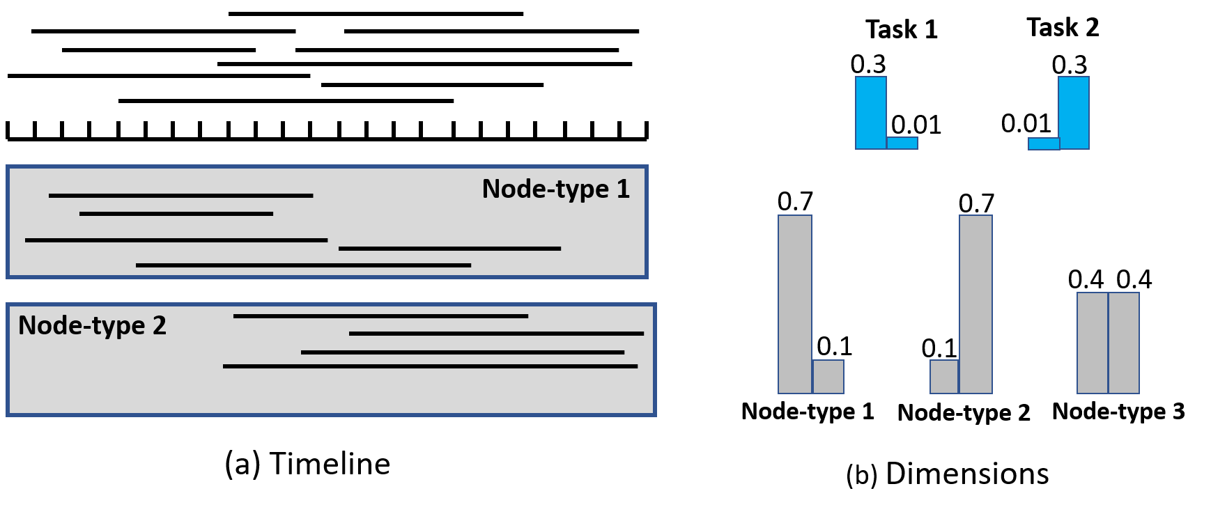
Figure 4: Illustration of deficiencies of penalty-based mapping. In part (a), tasks mapped to the first node-type are mainly active in the earlier segments of the timeline, whereas those mapped to the second are mainly active in the later segments, leading to resource wastage. In part (b), taking $D=2,m=3$ and $T=1$, resource demands/capacities along the two dimensions are shown. PenaltyMap would map tasks 1 and 2 to node-types 1 and 2, respectively, thereby utilizing two nodes, one from each type, whereas both can be accommodated in a single node of node-type 3.

V Linear Programming Based Mapping

While the penalty based mapping works reasonably well in practice, there are certain deficiencies in the strategy and we design an improved mapping based on linear programming.

V-A Penalty Based Mapping: Deficiencies

The penalty-based strategy makes the node-type choices for the tasks independent of each other, optimizing on an individual basis without considering the interactions. The lack of a collective analysis may lead to wastage of resource capacities, resulting in sub-optimal packing and higher cost.

There are two aspects to the issue, pertaining to the timeline and the resource dimensions. Firstly, tasks mapped to a node-type may be predominantly active only at certain segments on the timeline and less active at others. When the group of tasks get placed in nodes of the given type, the resource capacity gets wasted at the latter segments. Secondly, tasks with high demand along a particular dimension $d$ (say memory) are likely to get mapped to a node-type with higher capacity along $d$, wasting the capacity along the other dimensions. Figure 4 illustrates the two aspects. In addition, the node-type is selected based on normalized demands in an aggregated manner, ignoring the effect of individual dimensions.

V-B Linear Programming

We can address the above issues and find an improved mapping via linear programming (LP). Let $\pi:{\cal U}\rightarrow{\cal B}$ be any task to node-type mapping. Consider executing the two-phase algorithm (Figure 3) with the given mapping $\pi$ (instead of penalty-based mapping), followed by the same greedy placement for each node-type. Let $S_{\rm\pi}$ be the solution output by the algorithm. Using a proof similar to that Lemma 1, we can show the following lower-bound, denoted ${\rm LB}(\pi)$:

$${\tt cost}(S_{\rm\pi})\geq\sum_{B}\max_{t,d}\sum_{u\in V_{B}^{\rm\pi},u\sim t}\frac{{\tt dem}(u,d)}{{\tt cap}(B,d)},$$

where $V_{B}^{\rm\pi}$ is the set of tasks mapped to $B$ under $\pi$. Then, ${\tt cost}({\tt opt})$ is at least the minimum lower-bound over all the possible mappings:

$${\tt cost}({\tt opt})\geq\min_{\pi}{\rm LB}(\pi).$$

Our goal is to find the mapping $\pi$ with the least lower-bound ${\rm LB}(\pi)$. The goal can be accomplished via integer programming. We introduce a variable $x(u,B)$ for each pair of task and node-type, representing whether $u$ is mapped to $B$. We add a variable $\alpha_{B}$ for each node-type $B$, capturing the contribution from the node type to the lower-bound:

$$\sum_{B}\max_{t,d}\sum_{u\in V_{B}^{\rm\pi},u\sim t}\frac{{\tt dem}(u,d)}{{\tt cap}(B,d)}.$$

The integer program is shown below.

$$\min \sum_{B}{\tt cost}(B)\cdot\alpha_{B}$$

$$\forall u: \sum_{B}x(u,B)=1$$ (4)

$$\forall(B,t,d): \sum_{u\sim t}x(u,B)\cdot\frac{{\tt dem}(u,d)}{{\tt cap}(B,d)}\leq\alpha_{B}$$ (5)

$$\forall(u,B): x(u,B)\in\{0,1\},$$ (6)

where the first and the last constraint ensure that $u$ is mapped to exactly one node-type. Once the values of $x(u,B)$ are fixed, the optimal value for $\alpha_{B}$ is automatically the contribution of $B$. Thus, the integer program yields the desired mapping.

Unfortunately, it is prohibitively expensive to solve integer programs even on moderate size inputs. So, we resort to linear programming by relaxing the integrality constraint (6) as:

$$\forall(u,B):\quad 0\leq x(u,B)\leq 1.$$ (7)

Let $x^{*}(u,B)$ be the optimal LP solution. The objective value provides a lower-bound on ${\tt cost}({\tt opt})$.

V-C LP Rounding

In contrast to the integer program, LP produces a fractional solution: for each task $u$, the solution consists of a distribution (vector) over the node-types $[x^{*}(u,B)]$ summing to $1$, where $x^{*}(u,B)$ is the fractional extent to which $u$ is assigned to $B$. We design a procedure for transforming (rounding) the fractional solution into an integral solution. The procedure is based on a critical observation that the solution $x^{*}$ would be nearly integral, when $n$ is large enough.

Lemma 4.

In the solution $x^{*}$, the number of variables $x^{*}(u,B)$ with non-integral values is at most $n+mTD$.

Proof.

Assume that $x^{*}$ is an extreme point (or basic feasible) solution. The number of variables is $nm+m$ and so, at least as many constraints have to be tight [23]. Of these, $n+mTD$ can be from the constraints (4) and (5), and the rest must come from (7). Hence, at most $(n+mTD-m)$ of the $nm$ variables of the form $x(u,B)$ can be proper fractions. ∎

The lemma shows that of the $n\cdot m$ variables $x^{*}(u,B)$, most would be integral, when $n\gg TD$. From our experimental study, we observe that the above phenomenon manifests strongly in practice (irrespective of the values of $n$ and $TD$). For a task $u$, let $x_{\max}(u)=\max_{B}x^{*}(u)$ denote the maximum extent to which the task is assigned to a node-type. In the worst case, the solution can assign $u$ to an extent of $1/m$ to each node-type. However, the results show that $x_{\max}(u)=1$ or close to $1$ for vast majority of tasks. Meaning most of the tasks get assigned to a single node-type, or show a clear preference for a particular node-type. Figure 5 provides an illustration by considering a sample input from the experimental study.

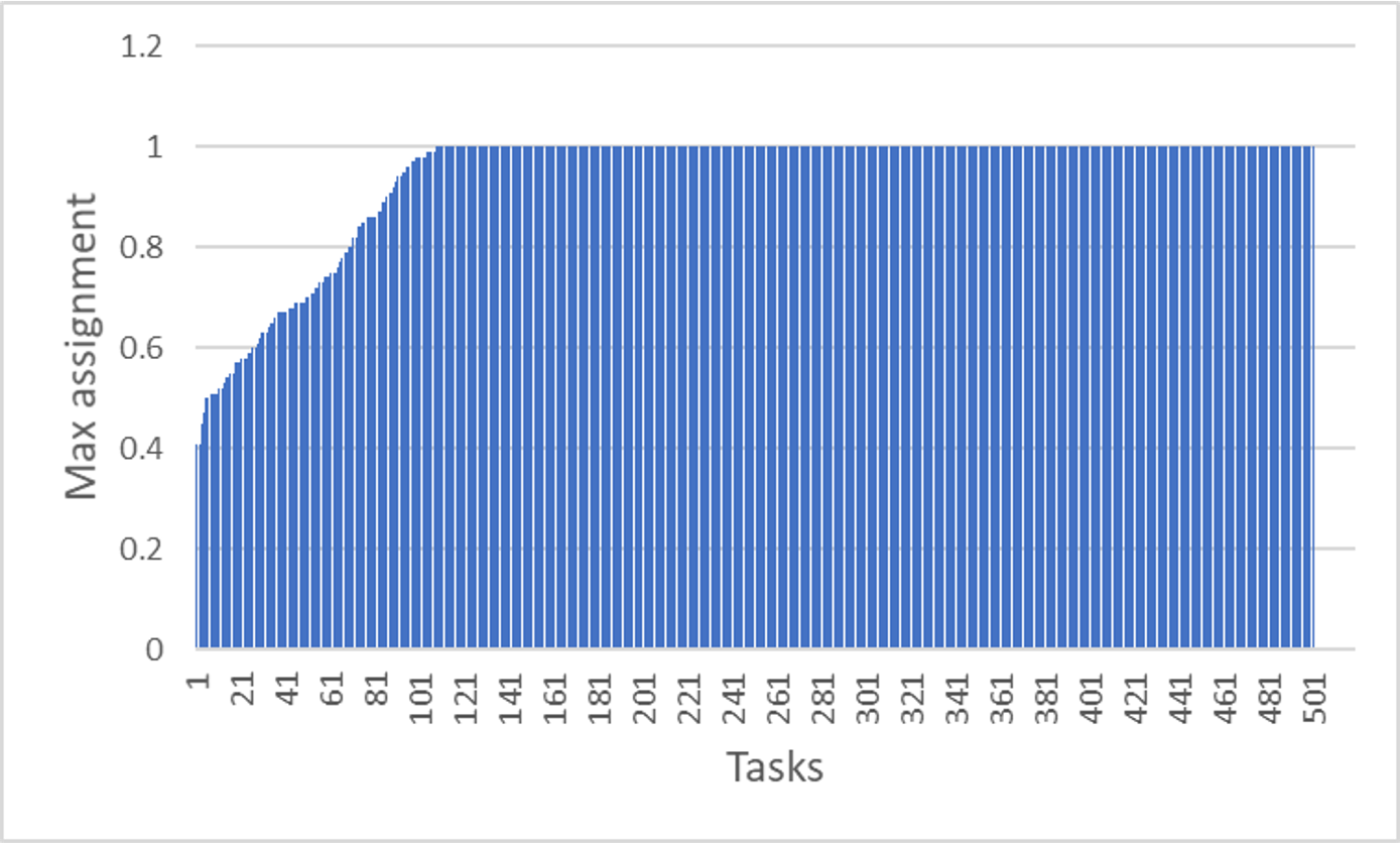
Figure 5: Illustration for near-integrality using a sample input from our experimental study with $n=500,m=10,D=5$ and $T=24$. The X-axis shows the tasks $u$ and the Y-axis shows $x_{\max}(u)$. Tasks are sorted by their value for the ease of visualization. We see that most of the tasks are assigned to a single node-type or show a clear preference for a particular node-type (the one receiving the maximum assignment)

Based on the above observation, we employ a simple, but effective, rounding heuristic: map each task $u$ to the node-type $B$ to which the task is assigned to the maximum extent:

$$\pi_{\rm LP}(u)=\operatorname*{argmax}_{B}\quad x^{*}(u,B).$$

Given the mapping, we partition the tasks according to the node-types and treat each node-type independently, using the same greedy placement heuristic as in PenaltyMap and obtain a solution $S_{\rm LP}$.

Analysis. The analysis of LP-map procedure is similar to that of PenaltyMap and a sketch is provided below. For any task $u$, there must be at least one node-type $B$ with $x^{*}(u,B)\geq 1/m$. Thus, the rounding incurs a loss by a factor of at most $m$. This fact combined with a proof similar to that of PenaltyMap can be used to show that that solution output by the LP-map satisfies:

$${\tt cost}(S_{\rm LP})\leq{\tt cost}({\cal B})+(2Dm)\cdot{\tt cost}({\tt opt}),$$

yielding an approximation ratio of $O(Dm)$. The solutions are much closer to the optimal in practice, with the margin being no more than $30\%$ in our experiments.

Mapping Phase: Construct the linear program and derive the solution $x^{*}$. For each task $u$: Map $u$ to $\pi_{{\rm LP}}(u)=\operatorname*{argmax}_{B}~{}x^{*}(u,B)$ Placement Phase: $R={\cal U}$    // Remaining tasks. Sort the node-types $B$ in decreasing order of $\frac{\sum_{d}{\tt cap}(B,d)}{{\tt cost}(B)}$. For each node-type $B$ in the above order: Initialize solution $S_{B}=\emptyset$ Let $V_{B}^{\rm LP}$ be the set of tasks mapped to $B$. Let $U=V_{B}^{\rm LP}\cap R$  // Mapped to $B$ and remaining Sort $U$ in the increasing order of start timeslots. For each task $u$ in the above order: If $u$ can fit in some node in $S_{B}$: Among the feasible nodes, place $u$ in the node purchased the earliest. Else: Purchase a new $B$-type node $b$ and place $u$ in it. // Cross node-type filling or piggy-backing Sort the tasks $u$ in $R$ in increasing order of $h_{\rm avg}(u,B)$. For each task $u$ in $R$ in the above order If $u$ can fit in some node in $S_{B}$: Among them place $u$ in the node purchased the earliest. Delete all the tasks placed in this iteration from $R$ Output: $S_{\rm LP}=\bigcup_{B}S_{B}$.

Figure 6: Algorithm LP-map with cross node-type filling

V-D Cross Node-Type Filling

The placement procedure is maximal in the sense that for any node-type $B$, it opens a new node for a task $u$ only when it cannot fit any of the nodes purchased already. However, the heuristic may leave empty spaces that can be filled by tasks of other node-types. We present a cross node-type filling method that reduces the overall cost by placing tasks mapped to the other node-types in the above empty spaces.

Suppose we have processed node-types $B_{1},B_{2},\ldots,B_{k}$ and let $S$ denote the set of nodes purchased already. Let $R$ denote the set of remaining tasks that are yet to be placed (these would be mapped to node-types $\geq k+1$). We wish to place as many tasks from $R$ in the nodes found in $S$. We employ a greedy heuristic for this purpose. We sort the tasks $u\in R$ in the increasing order of $h_{\rm avg}(u,B_{k})$, intuitively, arranging the task in terms of the space they would occupy. For each task $u$ in the above order, we check if $u$ can be placed in some node in $S$ without violating the feasibility constraint and if so, we place it in node purchased the earliest. The process is repeated till all the tasks are placed.

In the above process, tasks mapped to a node-type $B$ get an opportunity to piggy-back on the nodes purchased for the earlier node-types. Thus, the tasks mapped to later node-types are more likely to piggy-back and so, the ordering of the node-types is important. We sort the node-types in the decreasing order of capacity to cost ratio: $\sum_{d}{\tt cap}(B,d)/{\tt cost}(B).$ Intuitively, the ratio measures the capacity offered per unit cost and the sorting puts less cost-effective node-types later in the ordering, giving more opportunity for their tasks to piggy-back. A pseudo-code is presented in Figure 6. For each node-type $B$, the tasks that are mapped to $B$ are first placed, and then, the remaining tasks (mapped to later node-types) are accommodated as much as possible. The cross node-type filling method can also be applied to penalty based mapping (or to any other mapping strategy).

Time Complexity. The LP is designed to only find the task to node-type mapping, rather than a full solution encoding the placement of tasks in nodes. Consequently, the size of the LP is fairly small with the number of variables constraints being $O(nm)$ and $O(mTD)$, respectively. Interior point methods can converge in polynomial time and the execution time depends on the solver’s performance. Given the LP solution, the time complexity of the rest of the procedure is similar to that of PenaltyMap: the mapping takes time $O(n\cdot m)$, whereas placement takes time $O(n\cdot|S|\cdot D\cdot T)$, resulting in a total execution time of $O(n\cdot m+n\cdot|S|\cdot D\cdot T)$.

VI Experiments

VI-A Set-up

System. A machine with 2.5 GHz, Intel Core i7, 16GB memory and running macOS version 10.15.2 was used for running experiments implemented in python 3.8.7. We use python-mip package [33] with CBC solver for solving LP.

Google Cloud Trace 2019 (GCT 2019). GCT-2019 is used for real-world evaluation. 10M collection events (begin and end events of groups of tasks) and all machine-types (node-types) available for a single cluster (labeled “a”) [31] were sampled using BigQuery. Demand and capacity are two-dimensional (CPU and memory) and normalized in the trace. Entries with missing fields are purged from sampled trace. Time-stamps are converted to seconds. Task start and end times are discovered using task creation and end events. Thus, the task intervals, demands and capacities are drawn from the real trace. The node-type cost is generated synthetically (see below), and using publicly available pricing coefficients [32]. The processed data contains about 13K tasks and 13 node-types. Given $n$ and $m$, which is one experimental scenario, we construct an input instance by randomly sampling $n$ tasks and $m$ node-types from this processed data. Results are average across $5$ such random input instances per scenario. Timeline trimming is performed as discussed in Section II.

TABLE I: Default values for parameters

Parameter	Traces	Value
$n$	Both	1000
$m$	Both	10
T	Synthetic	24
Capacity	Synthetic	[0.2, 1.0]
Demand	Synthetic	[0.01, 0.1]
Dimensions	Synthetic	5

Synthetic Data. The GCT-2019 trace is $2$-dimensional and the task demands are fixed and small compared to node-capacities. In order to explore higher dimensions and different demand categories, we setup a synthetic benchmark using a random generator with inputs $n$, $m$, $D$, $T$, and intervals for demand and capacity of the form $[a,b]\subseteq[0,1]$. Each of the $D$ components of demand and capacity is uniformly and independently selected from its respective interval. For each task $u$, $[s(u),e(u)]$ is uniformly selected from $[1,T]$. We fixed $T=24$ and capacity interval as $[0.2,1]$. We pick $D\in\{2,5,7\}$, $m\in\{5,10,15\}$, demand intervals from $\{[0.01,0.05],[0.01,0.1],[0.01,0.2]\}$, and $n$ as per the experiment. Unless specified, default values used in specific experiments are shown in Table I. As in GCT-2019, for each scenario, results are averaged over 5 random inputs and timeline trimming is performed.

Cost-model. Node-type cost is computed as follows:

$$cost(B)=\sum_{d\in[1,D]}{c_{d}\cdot cap(B,d)^{e}}\vspace{-0.1in}$$ (8)

where $c_{d}$ is the coefficient for the resource component $d$ and the exponent $e$ is a measure of cost sensitivity to the changes in the resource quantities. We shall consider two cost models: homogeneous linear and heterogeneous. In the former, the coefficients and the exponent are set to one. In the latter, the coefficients are set heterogeneously and the exponent is varied to simulate non-linearity: (i) when $e=1$, the per-unit rate (cost/quantity) of a resource component remains constant; (ii) when $e<1$, the rate decreases with increase in the quantity; (iii) when $e>1$, the rate increases with increase in quantity.

Algorithms. Taking the penalty based mapping (PenaltyMap) as the baseline, we evaluate the LP based mapping (LP-map), LP based mapping with cross node-type filling (LP-map-F) and penalty based mapping with cross node-type filling (PenaltyMap-F).

For PenaltyMap and PenaltyMap-F, we report the minimum cost obtained from four (i.e. two mapping and two fitting policies described in Section III) combinations each. Similarly, for LP-map and LP-map-F, we take the minimum cost from two fitting policies respectively.

Linear Programming Lowerbound. We use the linear program discussed earlier (Section V-B) to derive a lowerbound (LB) on the cost of the optimal solution. The cost of solutions $S$ output by the algorithms are normalized as ${\tt cost}(S)/{{\rm LB}}$, so that a normalized cost of $1$ means that $S$ is optimal.

VI-B Homogeneous Linear Cost-Model

As noted earlier, the homogeneous cost-model computes ${\tt cost}(B)$ by setting $e=1$ and $c_{d}=1$ (Equation 8).

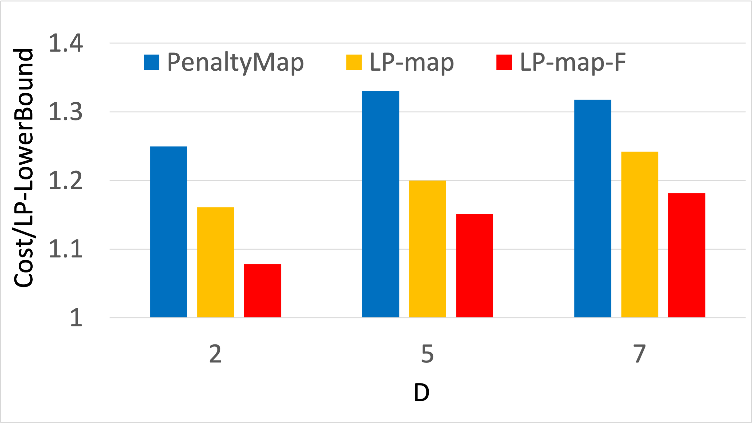
(a) Varying $D$. $m$=$10$, demand=$[0.01,0.1]$

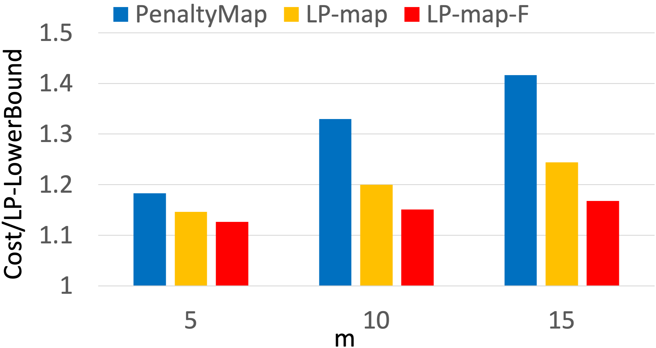
(b) Varying $m$. D=$5$, demand=$[0.01,0.1]$

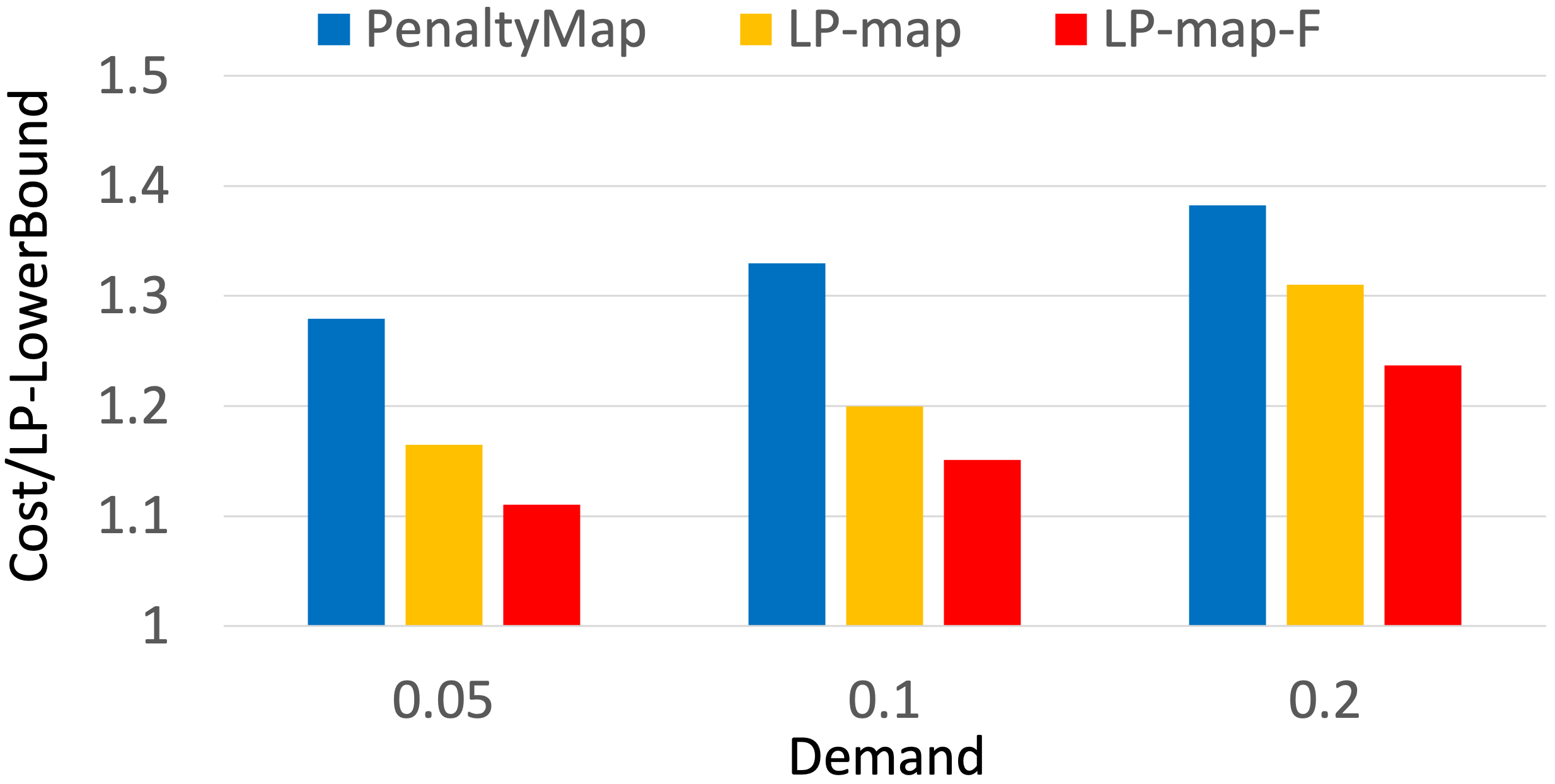
(c) Varying demand. $m$=$10$, $D$=$5$

Figure 7: [Synthetic-Homogeneous]: Comparison of algorithm when $m$, $D$ and demand are scaled.

VI-B1 Synthetic Trace

We first compare the three algorithms by scaling each of $D$, $m$ and the demand, fixing the other parameters.

Dimension. In Figure 7(a) $D$ is varied from $2$ to $7$. Compared to PenaltyMap, the LP-map strategy decreases the normalized cost by up to $0.13$ (or $13\%$), and LP-map-F plugs wastage by using the cross node-type filling, resulting in further reduction by up to $8\%$, taking the solution closer to the optimal. Overall, LP-map-F offers up to $17\%$ decrease in cost compared to PenaltyMap.

We also note that cost increases for all the mapping strategies as $D$ increases, since the instances become harder, but LP-map-F remains more resilient and remains within 20% of the lowerbound even for higher $D$, and is well within 10% for lower $D$, indicating that solution is close to optimal.

Node-type. In Figure 7(b) $m$ is varied from 5 to 15. Here again, LP-map-F outperforms PenaltyMap by up to 24% with cross node-type filling contributing up to 7% in this cost reduction. As a general trend, more node-types makes the mapping issue harder and the cost of all algorithms increase. The PenaltyMap algorithm is $18\%$ away from the lowerbound at $m=5$, and shoots to $41\%$ at $m=15$. In contrast, the LP-map-F algorithm remains stable resulting in only $4\%$ increase ($1.12$ to $1.16$)

Task demand. In Figure 7(c) task demand is varied from [0.01, 0.05] to [0.01, 0.2]. As in the two prior cases, LP-map-F performs the best in all the cases and stays under 25% of the lowerbound.

VI-B2 Real-trace Performance $-$ Scaling Tasks and Node-types

Google trace results are shown in Figure 8. First, we scale $n$ (Figure 8(a)) while keeping $m=10$ constant, and $D=2$ (CPU and memory). We see that LP-map outperforms PenaltyMap by large margins from $39\%$ to $156\%$ and produces near-optimal solutions, not more than $11\%$ away from the lowerbound. Our second experiment (Figure 8(b)) fixes $n=1000$ and varies $m$ from $4$ to $13$, wherein LP-map maintains $26\%-119\%$ lower cost than PenaltyMap and remains under $7\%$ of lowerbound.

In GCT-2019 trace, the task demands are small and so, the LP mappings are near-integral. Further, at smaller $D$, it is easier to fit the tasks, causing LP-map solutions to be very close to the optimal. The cross node-type filling has little room for improvement and hence LP-map-F exhibits similar performance as LP-map.

As $n$ increases, PenaltyMap has more tasks to map, due to which sub-optimal mappings get averaged, resulting in lesser capacity wastage and improved performance. However, as $m$ increases, the mapping issue becomes harder and the performance of the greedy heuristic degrades.

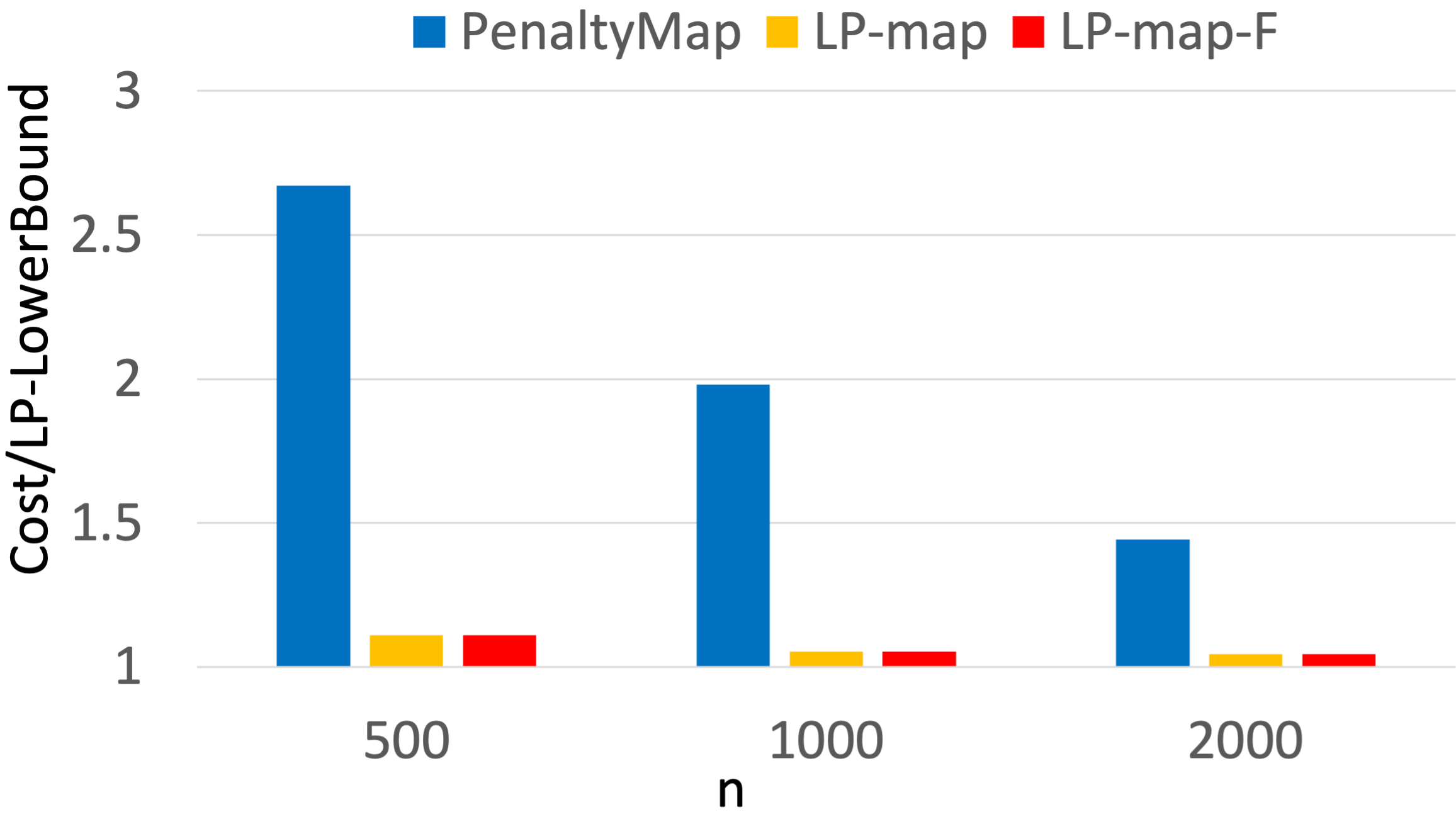
(a) Varying $n$. $m$=$10$

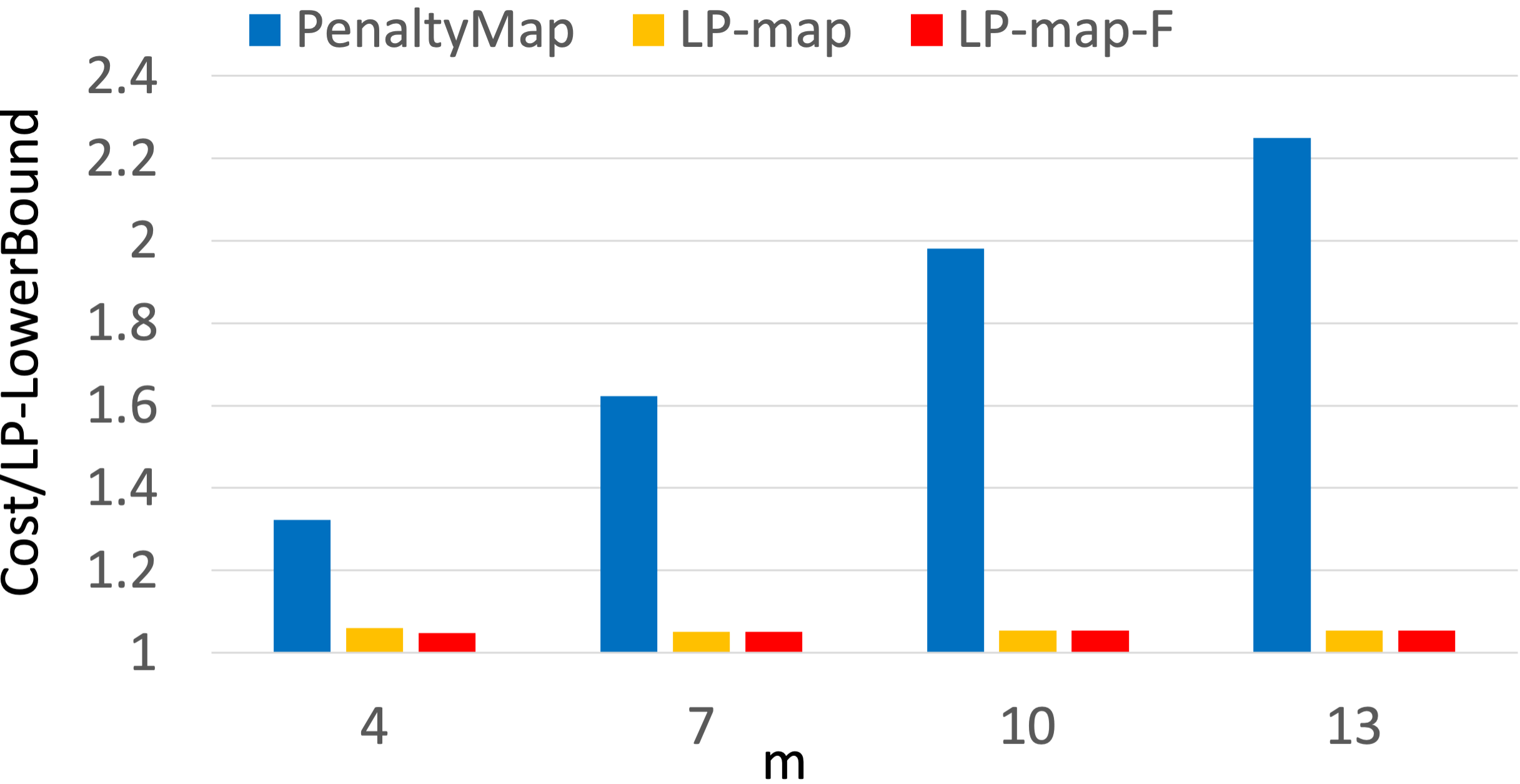
(b) Varying $m$. $n$=$1000$

Figure 8: [GCT-2019-Homogeneous]: Quality of solution when $m$ and $n$ are scaled.

VI-C Heterogeneous Cost-Model

Synthetic Data. We use a median point of $D=5$, $m=10$ and demand = $[0.01,0.1]$ for this experiment. Coefficients $c_{d}$ for the cost model (Equation 8) are generated randomly in the range of $[0.3,1.0]$. Further, we vary $e$ from $0.33$ to $3$. The results (Figure 9) show that LP-map-F offers up to $18\%$ gain over PenaltyMap for $e=1$, and up to $12\%$ gain $e<1$. Cross node-type filling provides a constant benefit of $2\%-3\%$ over LP-map for all values of $e$.

When $e>1$, the cost is skewed towards the largest resource component, and when $e<1$, the model tends towards uniform cost across the node-types (irrespective of their capacity). In both the cases, it is easier to map the tasks and hence, the greedy PenaltyMap gets closer to LP-map.

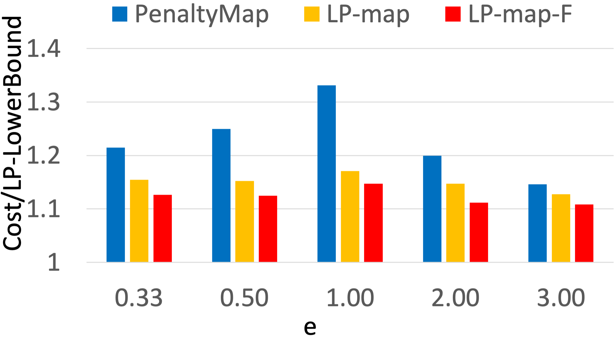
Figure 9: [Synthetic-Heterogeneous]: Varying $e$ for a given $m$.

Real-life Trace GCT-2019. For each node-type in GCT-2019, we use pricing coefficients from the Google pricing model [32], keeping the exponent $e=1$.

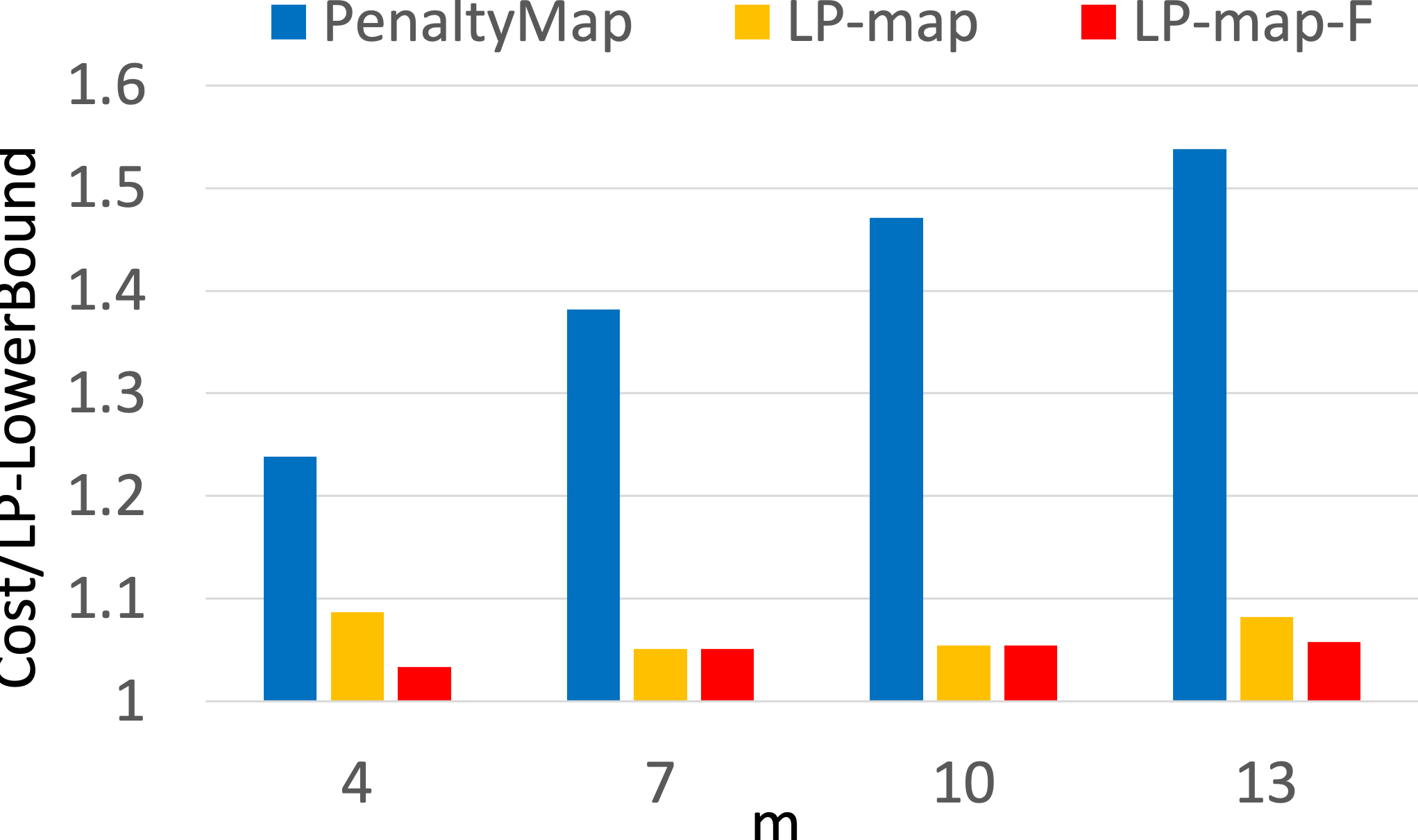
Figure 10: [GCT-2019-Heterogeneous]: Varying node-types ($n$=$1000$, $e$=$1$) using cost model with real-world coefficients.

Since, number of node-types has an important role in the quality of solution, we vary the node-types from $4$ to $13$. The results are shown in Figure 10. The performance of PenaltyMap is away from the lowerbound by $23\%$ at $m=4$, and degrades as $m$ increases, reaching $53\%$ at $m=13$. In contrast, LP-map-F gives high quality solutions staying close to $5\%$ of the lowerbound, while outperforming PenaltyMap by up to $48\%$. Cross node-type filling contributes up to $5\%$ in LP-map-F performance.

VI-D Cross Node-Type Filling

As mentioned earlier (Section V-D), cross node-type filling can be applied over PenaltyMap as well, and it is interesting to study the implications. Towards that goal, we augment PenaltyMap with the filling method to derive a PenaltyMap-F version, and evaluate on all the data points of the GCT-2019 trace experiments (Figures 8 and 10). We can see that the filling method offers $44\%$-$142\%$ gains over PenaltyMap.

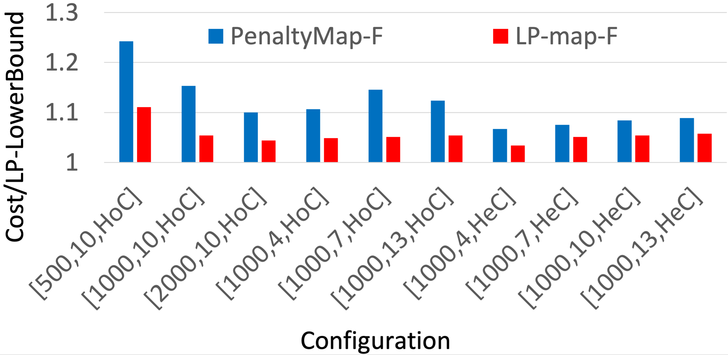
Figure 11: [GCT-2019 All-Scenarios]: Comparing PenaltyMap-F and LP-map-F.

Figure 11 compares PenaltyMap-F and LP-map-F, where LP-map-F outperforms PenaltyMap-F consistently with gains in the range $3\%$-$13\%$ establishing that an organic combination of LP-based mapping and cross node-type filling provides better solutions.

VI-E Running Time

We profiled the running time for all the algorithms on the largest configuration of 2000 tasks and 13 node-types from the GCT-2019 trace. We find that on the average, PenaltyMap takes about one second to produce a solution. Running time of the LP-based mappings could be split into the running time of the LP solver and the mapping phase. While the LP solver itself takes about 15 min, the mapping phase for both LP-map and LP-map-F takes about a second. Since our objective is cold-starting the cluster and cluster-sizing is an one-time computation, 15min is a very practical running time.

VI-F No-Timeline Scenario

Figure 1 illustrates the gains of incorporating the timeline into solution computation. To experimentally confirm these gains, we considered the configuration of 1000 tasks and 10 node-types from the GCT-2019 trace. We compared the cluster cost under timeline-aware and timeline-agnostic settings. For the former, we use the cost of LP-map-F solution (Figure 8(a)) and for the latter, we compute a lowerbound on the cost by treating the tasks to be always active. As expected, the latter produces higher cost, and we found that the factor is as high as $2$x on the average.

VII Conclusions

We introduced the TL-Rightsizing problem that reduces cluster cost by exploiting the time-limited nature of real-life tasks. We designed a baseline two-phase algorithm with an approximation ratio of $O(D\cdot\min(m,T))$, an improved LP-based mapping strategy and a cross-node-type filling method for further cost reduction. Experiments on synthetic and real-life traces demonstrate that the final algorithm produces solutions within $20\%$ of a lowerbound on the optimal cost. We identify two avenues of fruitful research. First is to further bridge the gap between the lowerbound and the solutions on the hard instances. Secondly, improving the approximation ratio would be of interest from a theoretical perspective. We also intend to work on enhancing the scheduler and auto-scaling algorithms to better leverage the output from TL-Rightsizing

References

- [1] NEC Wraps Red Hat OpenShift Into 5G Aspirations. https://www.sdxcentral.com/articles/news/nec-wraps-red-hat-openshift-into-5g-aspirations/2021/04/. Accessed: 2021-04-28.
- [2] A technical look at 5G energy consumption and performance. https://www.ericsson.com/en/blog/2019/9/energy-consumption-5g-nr. Accessed: 2021-04-28.
- [3] U. Adamy and T. Erlebach. Online coloring of intervals with bandwidth. In International Workshop on Approximation and Online Algorithms, 2003.
- [4] How the U.S. Air Force Deployed Kubernetes and Istio on an F-16 in 45 days. https://thenewstack.io/how-the-u-s-air-force-deployed-kubernetes-and-istio-on-an-f-16-in-45-days/. Accessed: 2021-04-28.
- [5] A. Bar-Noy, R. Bar-Yehuda, A. Freund, J. Naor, and B. Schieber. A unified approach to approximating resource allocation and scheduling. Journal of the ACM, 48(5):1069–1090, 2001.
- [6] How DENSO is fueling development on the Vehicle Edge with Kubernetes. https://www.cncf.io/blog/2019/10/01/how-denso-is-fueling-development-on-the-vehicle-edge-with-kubernetes/. Accessed: 2021-04-28.
- [7] C. Chekuri and S. Khanna. On multidimensional packing problems. SIAM Journal on Computing, 33(4):837–851, 2004.
- [8] Cost analysis of orchestrated 5G networks for broadcasting. https://tech.ebu.ch/docs/techreview/EBU_Tech_Review_2019_Lombardo_Cost_analysis_of_orchestrated_5G_networks_for_broadcasting.pdf. Accessed: 2021-04-28.
- [9] K. Elbassioni, N. Garg, D. Gupta, A. Kumar, V. Narula, and A. Pal. Approximation algorithms for the unsplittable flow problem on paths and trees. In Foundations of Software Technology and Theoretical Computer Science, volume 18, 2012.
- [10] Ivan Farris, Antonino Orsino, Leonardo Militano, Antonio Iera, and Giuseppe Araniti. Federated iot services leveraging 5g technologies at the edge. Ad Hoc Networks, 68:58–69, 2018.
- [11] E. Feller, L. Rilling, and C. Morin. Energy-aware ant colony based workload placement in clouds. In Grid Computing, 2011.
- [12] M. Gabay and S. Zaourar. Vector bin packing with heterogeneous bins: application to the machine reassignment problem. Annals of Operations Research, 242(1):161–194, 2016.
- [13] Daniel Gmach, Jerry Rolia, Ludmila Cherkasova, and Alfons Kemper. Workload analysis and demand prediction of enterprise data center applications. In 2007 IEEE 10th International Symposium on Workload Characterization, pages 171–180. IEEE, 2007.
- [14] H. Goudarzi and M. Pedram. Multi-dimensional sla-based resource allocation for multi-tier cloud computing systems. In Cloud Computing, 2011.
- [15] B. Han, G. Diehr, and Jack S J. Cook. Multiple-type, two-dimensional bin packing problems: Applications and algorithms. Annals of Operations Research, 50(1):239–261, 1994.
- [16] E. Jeannot, G. Mercier, and F. Tessier. Process placement in multicore clusters: Algorithmic issues and practical techniques. IEEE Transactions on Parallel and Distributed Systems, 25(4):993–1002, 2013.
- [17] B. Jennings and R. Stadler. Resource management in clouds: Survey and research challenges. Journal of Network and Systems Management, 23(3):567–619, 2015.
- [18] Arijit Khan, Xifeng Yan, Shu Tao, and Nikos Anerousis. Workload characterization and prediction in the cloud: A multiple time series approach. In 2012 IEEE Network Operations and Management Symposium, pages 1287–1294. IEEE, 2012.
- [19] H. Kierstead. Coloring graphs online. In A. Fiat and G. Woeginger, editors, Online algorithms: The state of the art. Springer, 1998.
- [20] KubeEdge: An open platform to enable Edge computing. https://kubeedge.io/en/. Accessed: 2021-04-28.
- [21] Kubernetes Auto-scaler. https://kubernetes.io/blog/2016/07/autoscaling-in-kubernetes/. Accessed: 2021-04-28.
- [22] W. Leinberger, G. Karypis, and V. Kumar. Multi-capacity bin packing algorithms with applications to job scheduling under multiple constraints. In International Conference on Parallel Processing, 1999.
- [23] J. Matousek and B. Gärtner. Understanding and using linear programming. Springer Science & Business Media, 2007.
- [24] Iyswarya Narayanan, Aman Kansal, and Anand Sivasubramaniam. Right-sizing geo-distributed data centers for availability and latency. In 2017 IEEE 37th International Conference on Distributed Computing Systems (ICDCS), pages 230–240. IEEE, 2017.
- [25] R. Panigrahy, K. Talwar, L. Uyeda, and U. Wieder. Heuristics for vector bin packing. Technical report, Microsoft, 2011.
- [26] B. Patt-Shamir and D. Rawitz. Vector bin packing with multiple-choice. Discrete Applied Mathematics, 160(10-11):1591–1600, 2012.
- [27] M. Rodriguez and R. Buyya. Deadline based resource provisioningand scheduling algorithm for scientific workflows on clouds. IEEE Transactions on cloud computing, 2(2):222–235, 2014.
- [28] P. Silva, C. Perez, and F. Desprez. Efficient heuristics for placing large-scale distributed applications on multiple clouds. In CCGrid, 2016.
- [29] Spring Batch on Kubernetes: Efficient batch processing at scale. https://spring.io/blog/2021/01/27/spring-batch-on-kubernetes-efficient-batch-processing-at-scale. Accessed: 2021-04-28.
- [30] Amir Varasteh, Basavaraj Madiwalar, Amaury Van Bemten, Wolfgang Kellerer, and Carmen Mas-Machuca. Holu: Power-aware and delay-constrained vnf placement and chaining. IEEE Transactions on Network and Service Management, 2021.
- [31] Google Cloud Trace 2019 helper document. https://drive.google.com/file/d/10r6cnJ5cJ89fPWCgj7j4LtLBqYN9RiI9/view. Accessed: 2021-02-28.
- [32] Google pricing model. https://cloud.google.com/compute/vm-instance-pricing. Accessed: 2021-02-28.
- [33] Python MIP solver. https://pypi.org/project/mip/1.12.0/. Accessed: 2021-02-28.
- [34] Jie Xu, Lixing Chen, and Shaolei Ren. Online learning for offloading and autoscaling in energy harvesting mobile edge computing. IEEE Transactions on Cognitive Communications and Networking, 3(3):361–373, 2017.
- [35] Maotong Xu, Sultan Alamro, Tian Lan, and Suresh Subramaniam. Cred: Cloud right-sizing with execution deadlines and data locality. IEEE Transactions on Parallel and Distributed Systems, 28(12):3389–3400, 2017.
- [36] Poonam Yadav, Julie A McCann, and Tiago Pereira. Self-synchronization in duty-cycled internet of things (iot) applications. IEEE Internet of Things Journal, 4(6):2058–2069, 2017.
- [37] Hao Yin, Xu Zhang, Hongqiang H Liu, Yan Luo, Chen Tian, Shuoyao Zhao, and Feng Li. Edge provisioning with flexible server placement. IEEE Transactions on Parallel and Distributed Systems, 28(4):1031–1045, 2016.